Distributed Fuzzy Cognitive Maps for Feature Selection in Big Data Classification

Abstract

The features of a dataset play an important role in the construction of a machine learning model. Because big datasets often have a large number of features, they may contain features that are less relevant to the machine learning task, which makes the process more time-consuming and complex. In order to facilitate learning, it is always recommended to remove the less significant features. The process of eliminating the irrelevant features and finding an optimal feature set involves comprehensively searching the dataset and considering every subset in the data. In this research, we present a distributed fuzzy cognitive map based learning-based wrapper method for feature selection that is able to extract those features from a dataset that play the most significant role in decision making. Fuzzy cognitive maps (FCMs) represent a hybrid computing technique combining elements of both fuzzy logic and cognitive maps. Using Spark’s resilient distributed datasets (RDDs), the proposed model can work effectively in a distributed manner for quick, in-memory processing along with effective iterative computations. According to the experimental results, when the proposed model is applied to a classification task, the features selected by the model help to expedite the classification process. The selection of relevant features using the proposed algorithm is on par with existing feature selection algorithms. In conjunction with a random forest classifier, the proposed model produced an average accuracy above 90%, as opposed to 85.6% accuracy when no feature selection strategy was adopted.

1. Introduction

In an age when big data is becoming increasingly popular, there is a huge amount of information that is redundant as well as irrelevant, which poses a challenge for academics and industry alike. The data that are gathered may be of high dimensionality, and, in most cases, not all of the features that are gathered are equally meaningful. Some of the features may be noisy, nonsensical, correlated, or unrelated to the task at hand. In most cases, high-dimensional data pose a problem for modeling tasks since the models are not always designed to cope with excessive amounts of inconsequential features, and this can reduce the performance of a predictive model. As a way of mitigating these problems, feature selection can identify relevant features and select them, eliminating nonessential or redundant features to maintain or improve classification accuracy [1]. Feature selection is a topic that has been studied intensively for a long time. Given the need to process massive amounts of data in a wide range of fields, the importance of this task has only grown. A second issue that practitioners must contend with is the lack of available computing resources. When dealing with huge amounts of data, the bulk of the approaches that are currently available for feature selection do not scale properly, and their efficiency may substantially decline to the point that they are no longer usable. Since present approaches are expected to prove inadequate for addressing the rising number of features found in big data, Bolón-Canedo et al. [2] concluded in their analysis of the most popular feature selection methods that a growing demand exists for scalable and efficient feature selection methods. Present approaches for feature selection are not likely to scale well when working with extensive data due to the fact that efficiency may considerably decline or the feature selection strategy may become inapplicable, which is the primary research need that has been identified.

Fuzzy Cognitive Maps (FCMs) [3] are systems inspired by human cognitive ability. FCMs employ a recursive learning procedure in order to learn about a given system and discover the various aspects of the system. An FCM is represented using a directed acyclic graph. The nodes in the graph represent the most important components of the system under consideration and the connections between the nodes represent the causal relationships between these concepts. Since FCMs represent the cause–effect relationships between attributes of a system, FCMs can be adopted to identify the features of a system that have maximum influence in the decision-making process. One of the major barriers in using FCMs is their inability to handle large datasets. This can be overcome by employing a distributed process to perform the FCM learning. The purpose of the current research was to look at the feasibility of using distributed FCMs to choose features from different data sources. The major contributions of this work are the following:

• A novel fuzzy cognitive map based technique to extract the most significant features in a dataset that contribute to decision making was introduced.
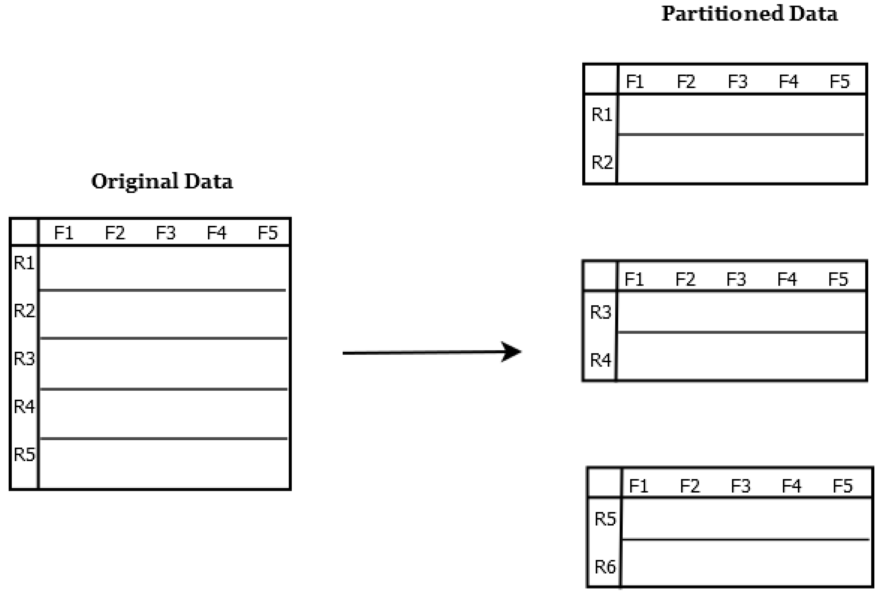
• The proposed model was implemented in a distributed manner, thus enabling the scalability of the feature selection algorithm.
• Comparison of the performance of the proposed distributed fuzzy cognitive map feature selection algorithm with other best-performing algorithms was carried out.

The paper is organized as follows: Section 2 provides insight into the current literature. Section 3 elaborates on the materials and methods used in the article. Section 4 demonstrates the results obtained and Section 5 is the performance analysis and discussion section. The paper’s conclusion is presented in Section 6.

2. Literature Review

A feature selection approach does not alter the original representation of the variables being analyzed; rather, it only selects a subset of them, as opposed to other dimensionality reduction approaches, such as those based on projection or compression. In this way, the variables retain their original meaning by preserving their original semantics and offering the advantage of being able to be interpreted by domain experts. Features can serve a variety of purposes, but the most important goals are (a) to reduce overfitting and improve model performance, that is, to achieve better prediction performance in supervised classification and better cluster-detecting performance in clustering; (b) to develop faster and more cost-effective models; and (c) to gain an understanding of the processes that produced the data. In contrast, the advantages of feature selection techniques are not without their downsides, as searching for a subset of relevant features introduces another layer of complexity to the modeling task. When the class labels of a feature set are known, feature selection strategies are categorized as supervised, and they are categorized as unsupervised when the class labels are unknown. There are three types of supervised feature selection strategy used in classification: filter, wrapper, and embedded methods [4]. The filter approach works as a preprocessing step and utilizes the general characteristics of the training data independent of the predictive model being used [5]. The wrapper selection method creates many models with different subsets of input features and selects the ones that yield the best performance [4]. A feature selection procedure that is embedded in a model’s training process is termed an embedded approach. Saeys et al. [6] investigated different ensemble feature selection techniques, which pool the strengths of different feature selection approaches to provide more reliable outcomes. Bolon-Canedo et al. [7] proposed an ensemble-learning-based feature selection to enhance the performance of micro-array data classification. There are other techniques that have been combined with feature selection, such as tree ensemble [8] and feature extraction [9]. Zang et al. suggested a two-stage feature selection algorithm by combining ReliefF and mRMR [10], while Akadi et al. [11] proposed a two-stage feature selection algorithm for genomic data by combining Minimum Redundancy–Maximum Relevance and Genetic Algorithm methods to obtain the optimal feature subset. Yuchen Jiang et al. [12] discussed three different approaches for feature selection in large-scale industrial processes for soft sensor construction. Karthik et al. [13] presented a method to improve the performance of open source software data prediction using Bayesian classification. Bhadoria et al. [14] discussed the use of an auto-encoder for dimensionality reduction based on bunch graphs. A new feature selection technique with ensemble learning, introduced by Hashemi et al. [15], converts the feature selection procedure into a multicriterion decision-making problem that is subsequently analyzed using the VICOR method. Kusy et al. [16] addressed the problem of feature selection as an aggregate of three cutting-edge filtration techniques: the linear correlation coefficient of Pearson, the ReliefF algorithm, and decision trees. Chellappan et al. [17] discussed the feature selection mechanisms available in the Apache Spark platform. Feature selection algorithms have been used in many real-world applications in the available literature, including intrusion detection [18], text categorization [19], email classification [20] microarray analysis [6], [21], information retrieval [22], etc.

Kosko introduced the concept of fuzzy cognitive maps in 1986 [3] as an extension of the Axelrod’s Cognitive Map proposal from 1976 [23]. FCMs provide a framework for representing complex systems by representing their components and causal relationships. FCMs add fuzzy logic to conventional cognitive maps. Due to their capacity to describe any complicated system, FCMs have attracted numerous researchers, and have been effectively used in a wide range of scientific domains. Using FCMs in the medical field, Giles et al. [24] studied the many causes of diabetes, Giabbanelli et al. [25] detected obesity through psychological behavior, and Papageorgiou et al. [26] used FCMs to investigate whether a person’s propensity to acquire breast cancer is affected by their family history of the condition. For crisis management decision making, Andreou et al. [27] suggested using FCMs as a tool for modeling political and strategic challenges. Zhai et al. [28] performed a credit risk assessment using FCMs [22]. The existing literature suggests many FCM expansions. Carvalho and Tome [29] presented a rule-based fuzzy cognitive map as an expansion of FCMs to include methods for dealing with feedback. Cognitive maps that deal with diverse meaning contexts were postulated by Salmeron [30]. Intuitionistic Fuzzy Cognitive Maps (iFCM) were developed by Iakovidis and Papageorgiou [31] to address experts’ reluctance in making decisions. Liu et al. [26] suggested an FCM variant that allows for the identification of dynamic causal links between the concepts. To represent dynamic systems, Aguilar [32] came up with the idea of dynamic random fuzzy cognitive maps (DRFCMs). The model of FCNs (fuzzy cognitive networks) was first proposed by Kottas et al. [33] based on the idea that equilibrium points always exist, while Chunying [34] presented Rough Cognitive Maps, a fuzzy cognitive map based on Rough Set Theory.

By building upon the relevant literature, this paper proposes an approach for the selection of features using distributed FCMs. The material and methods connected to distributed-FCM-based feature selection are presented in the next section. Next, the application of distributed-FCM-based feature selection is described and the obtained results are discussed. In the final section, conclusions and future challenges related to this issue are highlighted.

3. Materials and Methods

A framework for the selection of features using distributed FCMs is proposed in the current paper. Figure 1 depicts the overall workflow of the proposed method. In this method, the input dataset is used to construct a distributed FCM model, which is elaborated in Section 3.1. Section 3.2 explains how the constructed FCM is then used for feature selection, and the selected features are then passed onto the classification model for evaluation, as described in Section 3.3.

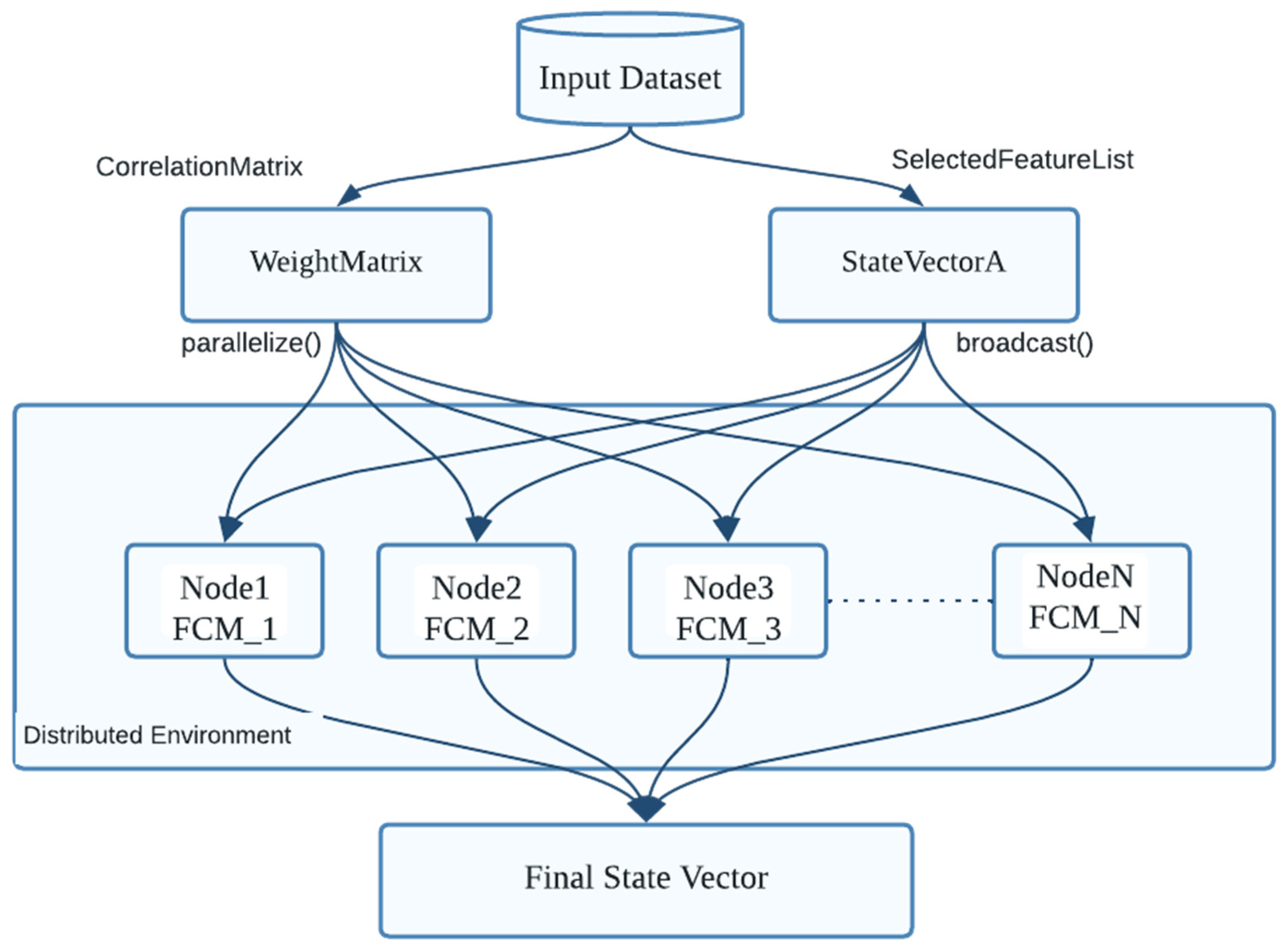
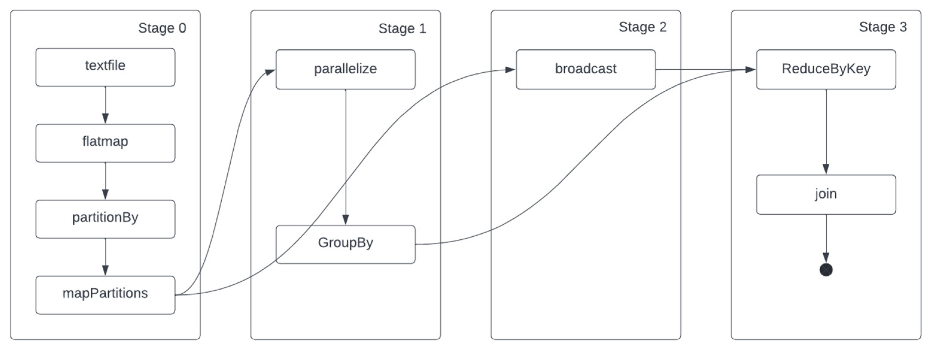
3.1. Distributed Fuzzy Cognitive Maps

A wide range of applications are available for FCMs. They provide a modeling technique that is useful to represent highly complex systems, and they can be also used to model uncertainties and improve accuracy in various application problems. A fuzzy cognitive map is a signed weighted digraph that includes fuzzy causal relationships between its nodes. An FCM consists of three components: concepts, state vector, and weight matrix. As part of the construction of an FCM, the state vector and weight matrix must be initialized, followed by training of the FCM model.

The state vector is composed of all the values of all the concepts in the system. Each positive value of the state vector depicts the inclusion of a particular feature. The weight matrix should be initialized to define the semantic properties of the dataset. A correlation matrix is used to initialize the weight matrix of the FCM. Within the weight matrix, each element represents the correlation coefficient between different features of the dataset. Each element is populated with the Pearson correlation coefficient value. To compute the correlation coefficient, the following formula is used:

$$r=\frac{{{\displaystyle \sum }}_i\left(x_i-\overline{x}\right)\left(y_i-\overline{y}\right)}{\sqrt{{{\displaystyle \sum }}_i{\left(x_i-\overline{x}\right)}^2}\sqrt{{{\displaystyle \sum }}_i{\left(y_i-\overline{y}\right)}^2}}$$

(1)

where $r$ is the correlation coefficient, $x_i$ is a sample’s x-variable values, $\overline{x}$ is their mean, $y_i$ is a sample’s y-variable values, and $\overline{y}$ is their mean. Regarding the values of $r$, r = 1 indicates a complete positive correlation, while r = −1 means a perfect negative correlation. The weight matrix and the state vector are stored in a resilient distributed dataset.

FCM learning is applied on the initial state vector using the following formula:

$$A_i^{\left(k+1\right)}=f\left(A_i^k+{\displaystyle \sum }_{j\ne i,j=1}^N{A}_j^k.W_{ij}\right)$$

(2)

where $W_{ij}$ is the weight of the link between concepts $C_i$ and $C_j$, and $A_i^{\left(k+1\right)}$ indicates the value of concept $C_i$ at step $k+1$.The sigmoid function is utilized as the threshold function f (x):

$$f\left(x\right)=\frac{1}{1+e^{-\lambda x}}$$

(3)

Iteratively, the state vector values are computed and the weight is modified until epsilon, a residual value that yields the smallest error difference between succeeding concepts, is attained. The equation used in each iteration step to update the weight matrix is given in Equation (4).

$$W_{ij}\left(k\right)=W_{ij}\left(k+1\right)+\left({\eta }_k\ast A_i^{\left(k-1\right)}-\left(A_j^{\left(k-1\right)}\ast W_{ij}^{\left(k-1\right)}\right)\right)$$

(4)

where Wji (k) represents the revised weight after the kth iteration. ${\eta }_k$ represents the value of the learning parameter in the kth iteration. Concept values fall within the interval [0,1], whereas weight values fall within the interval [−1,1].

A parallel learning process is proposed for FCM, as depicted in Figure 2. The parallelize function is given the weight matrix of the Spark’s Resilient Distributed Datasets (RDD) as input. Through the parallelize function, the weight matrix RDD is divided into sets of causal relations, and multiple new RDDs are created that contain subsets of weight matrix values for each node in the distributed system. As well as the weight matrix, the FCM learning requires the state vector. This requires the state vector to be available in all nodes where the weight matrix has been distributed. Therefore, we use the broadcast function on the state vector RDD, and the state vector is duplicated across all nodes. All distributed nodes cache the state vector. As the weight matrix RDD contains multiple rows and columns, it occupies very large amounts of space. However, the state vector RDD is a one-dimensional vector, so replicating it across the nodes will not impact memory capacity. FCM learning is applied at each node using Equation (2), and a partial result is generated. A final global solution, which is the final state vector, is obtained by combining these partial results.

The physical execution plan of the distributed FCM is represented using a directed acyclic graph, as depicted in Figure 3. The dataset is read by the compiler and stored into the Hadoop distributed file system (HDFS). The weight matrix and the state vector are computed from the dataset. The weight matrix is passed to the parallelize function where it is distributed into chunks of data using a hash function and sent to each node in the distributed system. The state vector is broadcasted across the nodes using the broadcast() method. The FCM model performs its computations in each individual node and separate results are produced. These results from multiple nodes are then passed to the reduce function wherein they are aggregated based on their key values. The user is subsequently presented with the final output.

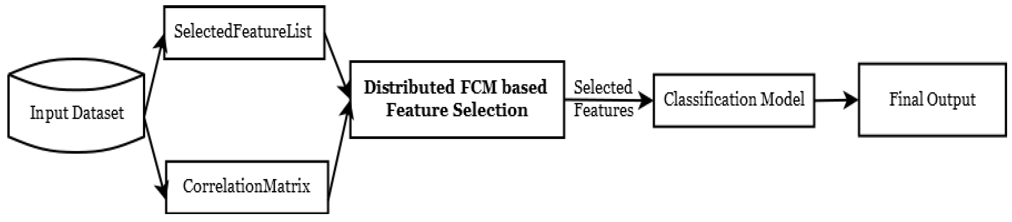
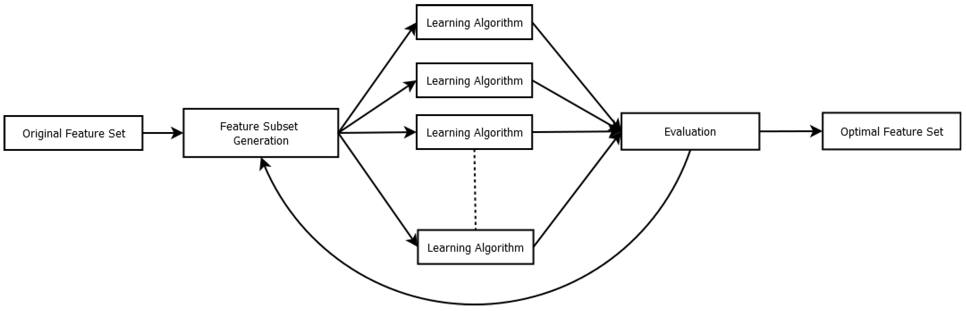
3.2. FCM-Based Feature Selection

In order to extract the most significant features using FCM, a causal relationship graph is constructed with the features as the nodes of the graph. The presence of a specific feature is indicated by a positive value in the state vector and the absence of the feature is indicated by 0. A correlation matrix is used to initialize the weight matrix of the fuzzy cognitive map. During FCM learning process in each iteration different combinations of features in the state vector is evaluated. The feature set that provides the best level of classification accuracy for the test data is chosen at each iteration and permanently added to the subsequent state vector. Classification accuracy (CA) is computed as a proportion of the accurately classified test instances:

$$\mathrm{Accuracy}=\frac{\mathrm{Successfully} \mathrm{classified} \mathrm{test} \mathrm{cases}}{\mathrm{Total} \mathrm{number} \mathrm{of} \mathrm{test} \mathrm{cases}} \ast 100$$

(5)

After the feature has been selected and added to the state vector, the same test is applied for the combinations of remaining features with the selected feature affixed at a particular position. As long as the target performance level is met or all features have been selected, these iterations are continued. Let F = {f1, f2, f3, f4, …, fn} be the set of all features in the dataset, S = {Ø} be initial set of selected features, A = {A1, A2, A3,…., An} be the state vector, and M be the weight matrix for the FCM. In each iteration, a different set of feature values in the state vector A are set to 1 and others are set as 0, for example, A = {01001010001}. The objective function for the FCM model is the maximization of the classification accuracy. The FCM model is trained using different combinations of the state vector A and the classification accuracies are computed based on Equation (5). The feature set A that gives the highest classification accuracy is selected and added to the selected feature set S. The iterations are continued until either the desired classification accuracy has been achieved or all the features in F have been selected at least once.

3.3. Classification Model

For the performance analysis of proposed model, the classification algorithms Naïve Bayes, Decision Tree, Random Forest, Multilayer Perceptron, and Logistic Regression were used. The distributed versions of the classification algorithms were used. The datasets were converted into pairs of feature vectors and class labels using the VectorAssembler method in spark. Since all the datasets were numerical datasets, no other preprocessing steps were necessary in order to process the datasets. The datasets were partitioned into different subsets and spread across different nodes. In the distributed Naïve Bayes classifier, the class labels and feature vectors are mapped together and distributed across nodes and a hash function is used to determine the conditional probability of the features, which is used to produce a probability table. The probability table is utilized in order to classify the dataset. In the distributed Decision Tree classifier, binary partitioning is done recursively to classify the features using a greedy algorithm. In the Random Forest model, each tree is trained using a different subset of the data. The Random Forest trees are actually trained on different parts of the same training set. A Tree Point structure is used to save the memory by storing the replica count of each instance in each subset. The number of mappers created is the same as number of trees in the Random Forest. Parallel training of a variable set of trees is optimized depending on memory constraints. Random Forest models reduce the risk of overfitting. Multilayer perceptron classifier (MLPC) is a feed-forward neural network classifier. MLPC has layered nodes. Network layers are completely linked. Input layer nodes represent input data. All other nodes translate inputs to outputs by linearly combining inputs with weights, bias, and an activation function. The model takes the composition of layers as input. While using the multinomial logistic regression model, a matrix of the number of outcome classes and the features is created and a Softmax function is used to model the outcome class’s conditional probabilities.

The algorithm corresponding to the proposed methodology is given in Algorithm 1. In the proposed algorithm, the accuracy threshold is the accuracy value obtained when the classifier is applied on the dataset without any feature selection performed. Our intention is to obtain better accuracy values. Another assumption is the epsilon threshold value.

Algorithm 1. Distributed Fuzzy Cognitive Map (FCM) algorithm for feature selection in big data
1	Initialize global variable FeatureVector to 0
2	procedure FCM()
3	{
4	Read the features in the dataset to a features variable
5	Compute the correlation matrix for the features and assign it to weight matrix
6	For all features[i] in features do
7	Initialize the StateVector with 1 for selected features and 0 otherwise
8	While(true)
9	Parallelize the WeightMatrix
10	Broadcast the StateVectorA
11	Update VectorA as weightMatrix * StateVectorA
12	Assign StateVectorA = updatedVectorA
13	Compute the classification Accuracy of updated StateVectorA
14	If(accuracy > accuracyThreshold)
15	Add the features in StateVectorA to FeatureVector
16	weightMatrix = updateWeights(weightMatrix)
17	epsilon = compute Epsilon()
18	if epsilon < threshold
19	break;
20	}

4. Results

The experiment was performed on a high-performance Hadoop cluster with one name-node server and two data-node servers with a combined capacity of 768 GB RAM and 144 core processors. The cluster supports Apache Spark 3.0.0 version. To determine the effectiveness and efficiency of the proposed model, 15 benchmark datasets available in the UCI machine learning repository [35], kaggle data repository, OpenML dataset repository, and PROMISE software dataset repository, which have been commonly used to evaluate feature selection models in the literature, were used.

The datasets used are summarized in

Table 1. Dataset description.

Sl.no.	Dataset	Instances	Features	Class
1	Breast Cancer Wisconsin (Diagnostic) Data Set	569	32	2
2	US Congressional Voting Records dataset	435	16	2
3	Pima Indians Diabetes dataset	768	8	2
4	Polycystic ovary syndrome (PCOS) dataset	541	45	2
5	Parkinson Disease Detection dataset	197	23	2
6	Wine dataset	178	13	3
7	Zoo dataset	101	17	7
8	Connectionist Bench (Sonar, Mines vs. Rocks) Data Set	208	60	2
9	Lung Cancer Data Set	226	23	3
10	Climate Model Simulation Crashes Data Set	540	18	2
11	Scene dataset	2407	294	2
12	Page Blocks Classification Data Set	5473	10	5
13	kc1	2110	21	2
14	pc1	1109	21	2
15	cm1	345	35	2

. Various datasets with dimensionalities ranging from extremely low to very high and different sizes were taken into consideration to ascertain the performance of the proposed model on different types of dataset.

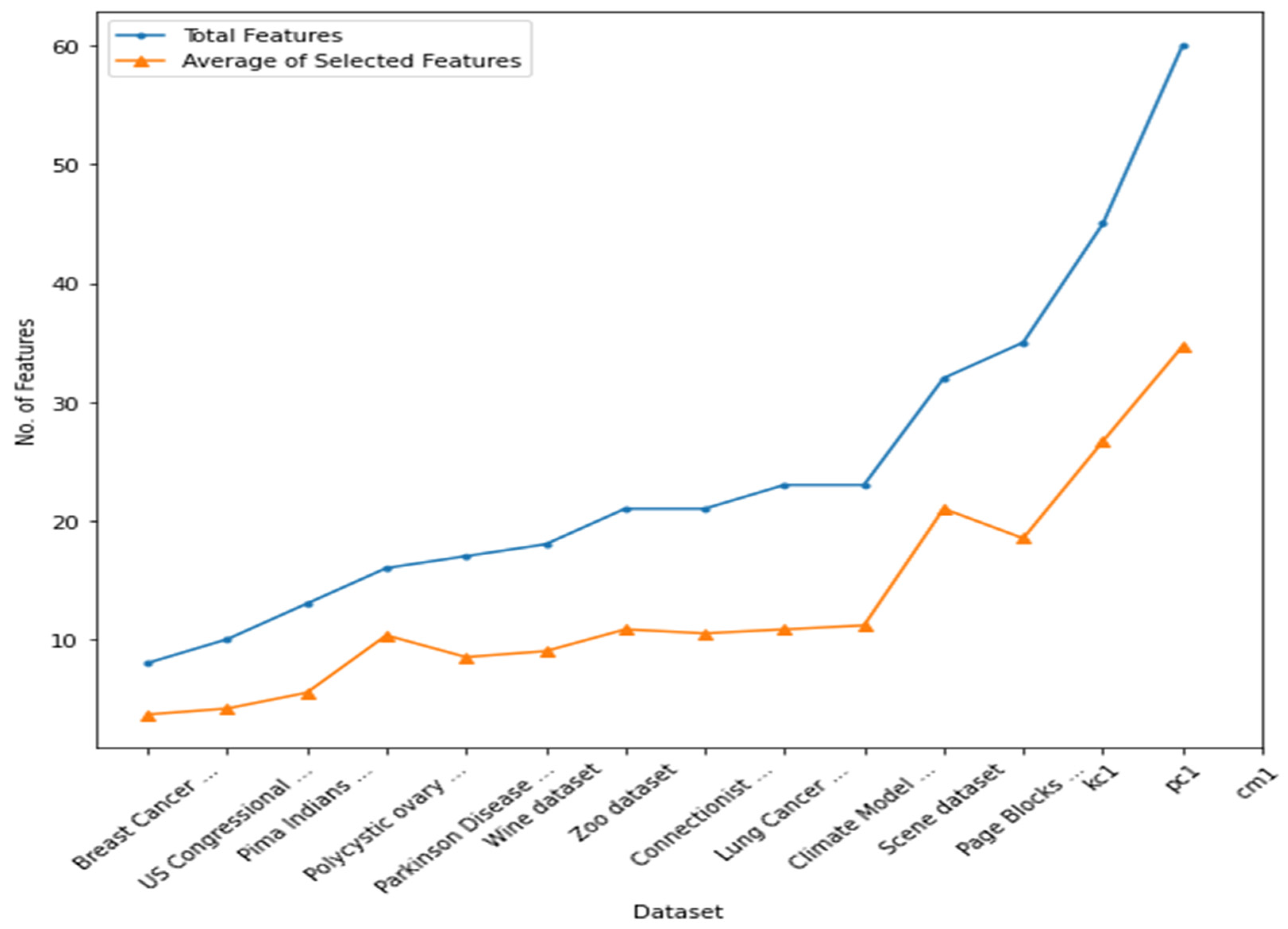
4.1. Total Number of Features vs. Average Number of Features

Figure 4 depicts the comparison between total number of features and average number of selected features from 20 independent runs of the proposed feature selection model. From the results, it can be deduced that the proposed model considerably reduced the number of features being selected. Only the most significant features that directly influenced the result were selected and the rest were discarded. The proposed model selected less than 50% of the total features in the dataset.

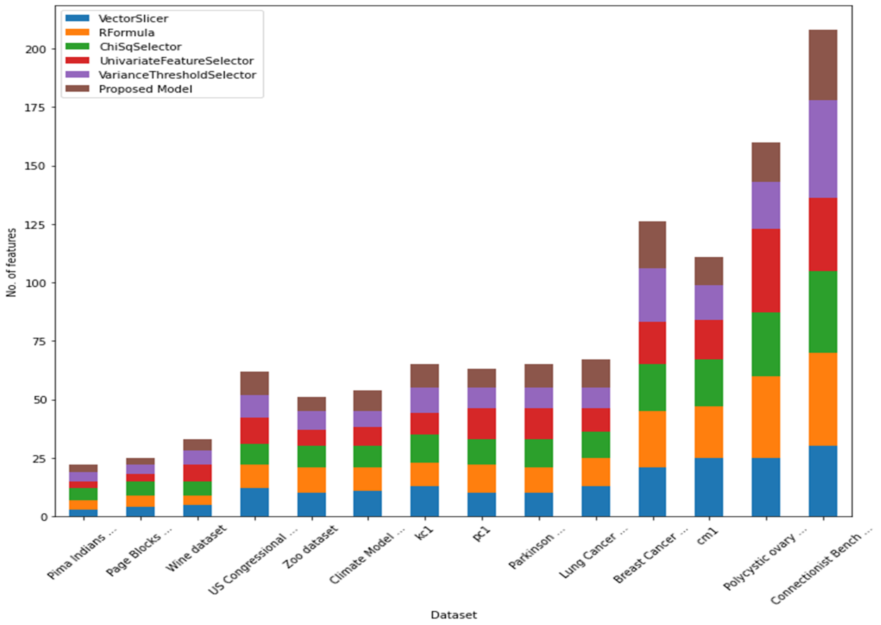
4.2. Proposed Feature Selection vs. Existing Feature Selection

A comparison of the performance of the proposed distributed FCM-based feature selection model against a number of state-of-the-art methods available in the Apache Spark [17] platform was also carried out. The model was compared with existing distributed feature selection methods such as VectorSlicer, RFormula, ChiSqSelectotr, UnivariateFeature Selector, and VarianceThreshold Selector in terms of how well it selected the optimal number of features, as depicted in

Table 2. Number of features selected by different feature selection algorithms.

Dataset	Vector Slicer	RFormula	ChiSq Selector	Univariate Feature Selector	Variance Threshold Selector	Proposed Model
Pima Indians Diabetes dataset	3	4	5	3	4	3
Page Blocks Classification Data Set	4	5	6	3	4	3
Wine dataset	5	4	6	7	6	5
US Congressional Voting Records dataset	12	10	9	11	10	10
Zoo dataset	10	11	9	7	8	6
Climate Model Simulation Crashes Data Set	11	10	9	8	7	9
kc1	13	10	12	9	11	10
pc1	10	12	11	13	9	8
Parkinson Disease Detection dataset	10	11	12	13	9	10
Lung Cancer Data Set	13	12	11	10	9	12
Breast Cancer Wisconsin (Diagnostic) Data Set	21	24	20	18	23	20
cm1	25	22	20	17	15	12
Polycystic ovary syndrome (PCOS) dataset	25	35	27	36	20	17
Connectionist Bench (Sonar, Mines vs. Rocks) Data Set	30	40	35	31	42	30

. The proposed model was capable of selecting the optimal number of features in most of the datasets considered.

Figure 5 depicts the comparison of the results of number of features selected by different distributed feature selection algorithms against the proposed model. The results demonstrated the proposed model’s supremacy across all datasets and its success in outperforming the other algorithms.

4.3. Performance Evaluation of the Proposed Feature Selection

A set of five classification algorithms, Naïve Bayes, Decision Tree, Random Forest, Multilayer Perceptron, and Logistic Regression were used to evaluate the efficiency of the optimal feature set obtained using FCM-based feature selection.

Table 3. Classification accuracies obtained for different classification algorithms.

Dataset	Naïve Bayes	Decision Tree	Random Forest	Multi-layer Perceptron	Logistic Regression
Breast Cancer Wisconsin (Diagnostic) Data Set	78.3	85.14	97.32	74.55	88.57
US Congressional Voting Records dataset	80.65	83.231	99.66	90.86	84.3
Pima Indians Diabetes dataset	64.84	72.72	80.5	66.06	75.36
Polycystic ovary syndrome (PCOS) dataset	66.38	77.8	88.97	85.14	90.65
Parkinson Disease Detection dataset	76.2	86.71	91.83	82.901	87.025
Wine dataset	80.97	79.7	93.34	87.26	82.36
Zoo dataset	67.55	72.53	89.36	84.321	79.015
Connectionist Bench (Sonar, Mines vs. Rocks) Data Set	61.23	76.66	86.47	69.8	80.704
Lung Cancer Data Set	70.4	80.5	88.63	76.04	83.9
Climate Model Simulation Crashes Data Set	72.84	80.97	92.41	86.32	89.01
Scene dataset	68.19	74.85	91.82	93.74	85.44
Page Blocks Classification Data Set	73.85	83.5	95.33	90.88	89.56
kc1	69.73	72.3	82.125	85.67	77.46
pc1	74.96	76.72	93.1	87.58	90.11
cm1	68.432	70.658	89.67	85.4	92.85

represents the accuracy values obtained for different classification algorithms when the datasets taken into consideration were evaluated after FCM-based feature selection. The results depict that the Random Forest algorithm tended to produce maximum accuracy values as compared to other classification algorithms. Random Forest algorithms use bootstrap aggregation and randomization in selection of data nodes during the construction of decision trees to obtain a high degree of predictive accuracy. The Random Forest algorithm also tends to have the capability to handle large datasets more efficiently compared to other classification algorithms; therefore, Random Forest was chosen as the classification model to evaluate the performance and efficiency of the proposed feature selection method. An ensemble of individual decision trees comprises the Random Forest algorithm. Each tree in the random forest produces a class prediction, and the class with the most votes becomes the prediction of the model.

Table 4. Results obtained from proposed FCM-based feature selection model.

Dataset	Accuracy	Accuracy after Feature Selection	Total Features	Selected Features
Breast Cancer Wisconsin (Diagnostic) Data Set	96.25	97.32	32	14
US Congressional Voting Records dataset	97.2	99.66	16	7
Pima Indians Diabetes dataset	78.9	80.5	8	3
Polycystic ovary syndrome (PCOS) dataset	86.02	88.97	45	17
Parkinson Disease Detection dataset	87.65	91.83	23	9
Wine dataset	92.6	93.34	13	5
Zoo dataset	88.15	89.36	17	6
Connectionist Bench (Sonar, Mines vs. Rocks) Data Set	75.3	86.47	60	26
Lung Cancer Data Set	83.5	88.63	23	10
Climate Model Simulation Crashes Data Set	88	92.41	18	9
Scene dataset	86.8	91.82	294	101
Page Blocks Classification Data Set	91	95.33	10	3
kc1	81	82.125	21	10
pc1	80	93.1	21	8
cm1	83	89.67	35	12

shows the results according to the average accuracy of the Random Forest classifier and optimal subset of features selected. The suggested model’s performance on classification tasks was evaluated using the Random Forest method, since it achieved the best classification results for the datasets under consideration. The results showed that the proposed model gave us good output results in identifying the optimal subset of features selected and showed improvements in classification accuracies for all datasets taken into consideration. Through the accuracy of classification, the suggested model obtained outstanding results while only selecting a relatively small percentage of the features in the dataset, thereby considerably reducing the amount of data to be processed.

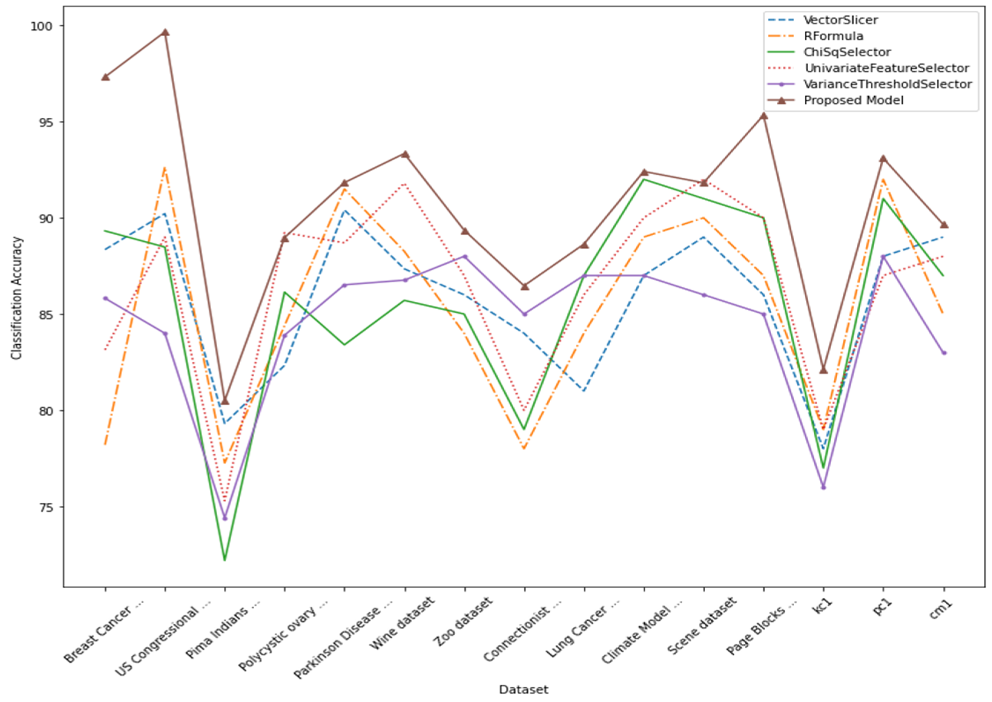
4.4. Performance Comparison with Existing Feature Selection Methods

The classification accuracy of the proposed model was compared with classification accuracies obtained after feature selection using state-of-the-art feature selection methods. The results obtained are depicted Figure 6. The results show that the proposed feature selection model produced better results for the datasets taken into consideration as compared to existing feature selection methods, namely VectorSlicer, RFormula, ChiSqSelector, UnivariateFeature Selector, and VarianceThreshold. The proposed model makes use of the accuracy values in order to determine the optimal feature set as opposed to using statistical methods to calculate the feature set; therefore, it acts as a good model for feature selection for classification tasks.

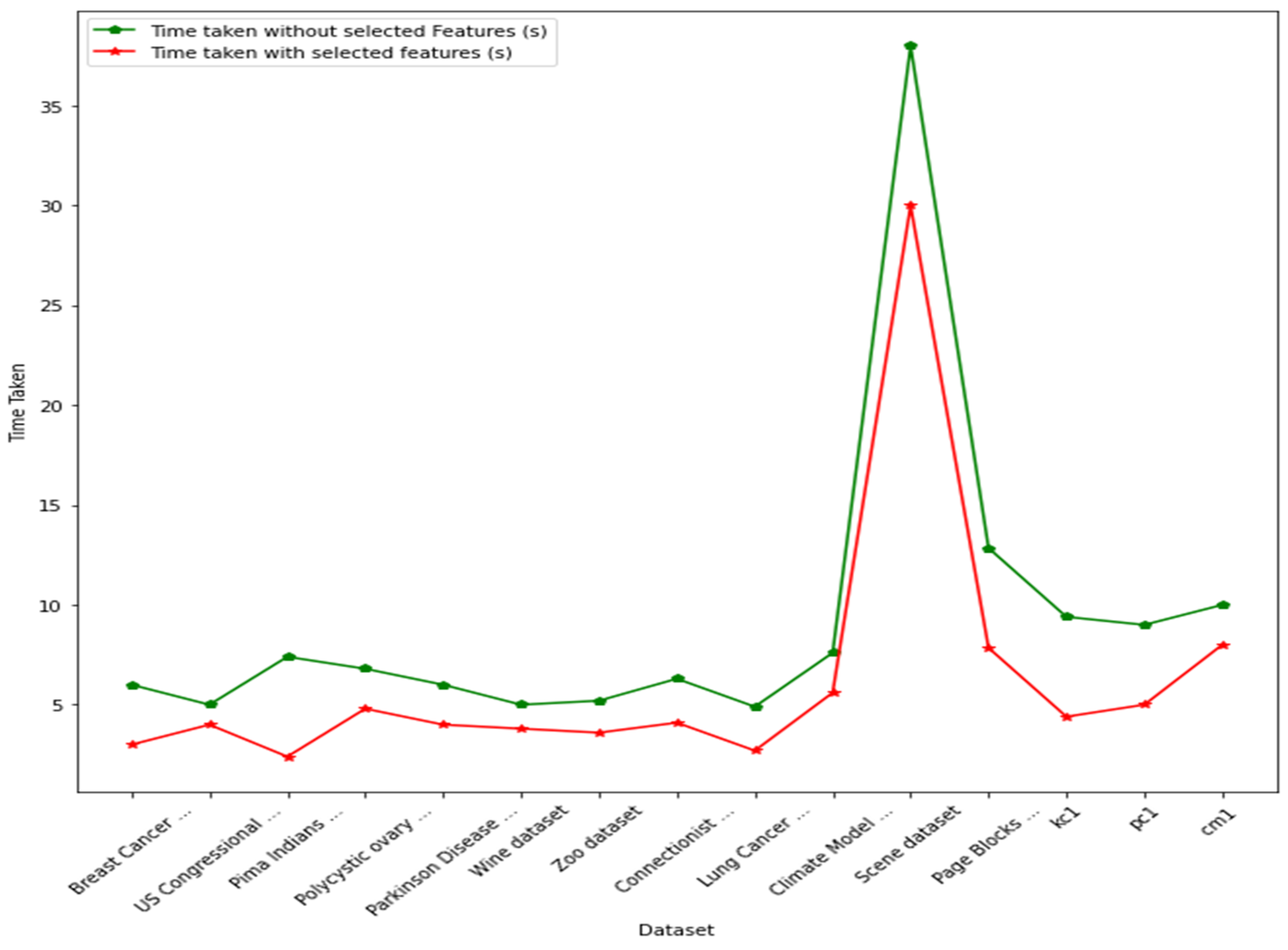
4.5. Comparison of Computational Time for Classification with and without Feature Selection

Figure 7 depicts the comparison of computational time of the model when feature selection was applied and when feature selection was not applied. From the results, it can be observed that applying the feature selection model along with classification considerably reduced the computational time. Using a feature selection method reduces the dimension of the feature space by selecting the most relevant features with respect to the problem under consideration, thereby reducing the computational load on the classification system.

5. Performance Analysis and Discussion

In the course of this investigation, a model for the selection of features based on a wrapper technique was adopted. The feature selection model used in previous studies is a sequential implementation of the wrapper technique, as illustrated in Figure 8. In the sequential technique, learning is conducted consecutively following feature subset generation, and if it does not pass the evaluation threshold, the feature subset generation is repeated; otherwise, the subset is chosen as the best feature set.

In this work, a distributed feature selection approach was adopted, as depicted in Figure 9. In the proposed model, a feature subset is generated and the efficiency of the selected feature subset is evaluated in a distributed manner by the learning algorithm. If the generated subset satisfies the evaluation threshold, it is selected as the optimal feature set; otherwise, a new feature subset is generated and the evaluation process continues. The dataset is partitioned into different chunks as part of the learning process of the feature selection model, as shown in Figure 10.

The performance of the proposed model was compared with existing distributed feature selection models, namely VectorSlicer, RFormula, ChiSqSelectotr, UnivariateFeature Selector, and VarianceThreshold Selector. Table 2 demonstrates that, across the majority of datasets, the minimum number of features was acquired by using the proposed distributed FCM-based feature selection technique. The datasets for which the proposed algorithm selected the smallest number of features has been highlighted. For all but three datasets, the proposed model chose the smallest number of features. The effectiveness of the optimum feature set acquired using FCM-based feature selection was evaluated using five classification algorithms: Naïve Bayes, Decision Tree, Random Forest, Multilayer Perceptron, and Multinomial Logistic Regression. After FCM-based feature selection, the datasets used for evaluation yielded accuracy values which are displayed in Table 3. The findings indicate that, compared to other classification methods, the Random Forest approach often yielded the highest accuracy scores for the considered datasets. The Random Forest method employs a majority agreement prediction technique, wherein a group of individual decision trees form an ensemble, thereby reducing the number of possible types of error and leading to higher accuracy of results. Hence, using the Random Forest algorithm, the performance of the proposed model was compared with existing feature selection algorithms. Figure 6 depicts the comparison of classification accuracies obtained when the proposed model was compared with existing methods. It can be noted that even though the number of features selected by the proposed model was not minimal in all the datasets, the figure depicts that the features selected were the optimal feature set, since the proposed model produced the best accuracy values as compared to other models.

6. Conclusions

Enormous amounts of high-dimensional data are prevalent in numerous fields, including social media, e-commerce, bioinformatics, healthcare, transportation, and online education. The preprocessing phase of feature selection has been widely employed to reduce the dimensionality of problems and increase the accuracy of classification. There has been an increase in the need for such approaches in recent years due to situations involving high numbers of input attributes and samples. In other words, the big data boom today has the resulted in the challenge of big dimensionality.

Featuring a distributed fuzzy cognitive map based feature selection method, this paper addressed the paramount need for a feature selection algorithm. The algorithm was tested on 15 benchmark datasets. A variety of comparisons were made with existing feature selection algorithms, including VectorSlicer, RFormula, ChiSqSelectotr, UnivariateFeature Selector, and VarianceThreshold Selector. The efficiency of the optimal feature set obtained was evaluated on different classification algorithms, namely Naïve Bayes, Decision Tree, Random Forest, MultiLayer Perceptron, and Logistic Regression. The results depict that the Random Forest algorithm produced the most accurate results for most of the datasets considered. The average accuracy was above 90% when using the Random Forest classifier along with the proposed feature selection method, in contrast to 85.6% without applying feature selection. The number of optimal feature sets selected was considerably less in the case of proposed model compared to the existing methods.

References

1. Guyon, I.; Elisseeff, A. An Introduction to Variable and Feature Selection. J. Mach. Learn. Res. 2003, 3, 1157–1182. [Google Scholar]
2. Bolón-Canedo, V.; Sánchez-Maroño, N.; Alonso-Betanzos, A. Recent advances and emerging challenges of feature selection in the context of big data. Knowl.-Based Syst. 2015, 86, 33–45. [Google Scholar] [CrossRef]
3. Kosko, B. Cognitive fuzzy maps. Int. J. Man-Mach. Stud. 1986, 24, 65–75. [Google Scholar] [CrossRef]
4. Kohavi, G.H.J.R. Wrapper for Feature Subset Selection. Artif. Intell. 1997, 97, 273–324. [Google Scholar] [CrossRef] [Green Version]
5. Bolón-Canedo, V.; Sánchez-Maroño, N.; Alonso-Betanzos, A. A review of feature selection methods on synthetic data. Knowl. Inf. Syst. 2013, 34, 483–519. [Google Scholar] [CrossRef]
6. Bolón-Canedo, V.; Sánchez-Maroño, N.; Alonso-Betanzos, A. An ensemble of filters and classifiers for microarray data classification. Pattern Recognit. 2012, 45, 531–539. [Google Scholar] [CrossRef]
7. Saeys, Y.; Abeel, T.; van de Peer, Y. Robust Feature Selection Using Ensemble Feature Selection Techniques. In Lecture Notes in Computer Science Book Series (LNAI); Springer Science: Berlin, Germany, 2008; Volume 5212. [Google Scholar]
8. Tuv, E.; Borisov, A.; Runger, G.; Torkkola, K. Feature selection with ensembles, artificial variables, and redundancy elimination. J. Mach. Learn. Res. 2009, 10, 1341–1366. [Google Scholar]
9. Vainer, I.; Kraus, S.; Kaminka, G.A.; Slovin, H. Obtaining scalable and accurate classification in large-scale spatio-temporal domains. Knowl. Inf. Syst. 2011, 29, 527–564. [Google Scholar] [CrossRef]
10. Zhang, Y.; Ding, C.; Li, T. Gene selection algorithm by combining reliefF and mRMR. BMC Genom. 2008, 9, S27. [Google Scholar] [CrossRef] [PubMed] [Green Version]
11. el Akadi, A.; Amine, A.; el Ouardighi, A.; Aboutajdine, D. A two-stage gene selection scheme utilizing MRMR filter and GA wrapper. Knowl. Inf. Syst. 2011, 26, 487–500. [Google Scholar] [CrossRef]
12. Jiang, Y.; Yin, S.; Dong, J.; Kaynak, O. A Review on Soft Sensors for Monitoring, Control, and Optimization of Industrial Processes. IEEE Sens. J. 2021, 21, 12868–12881. [Google Scholar] [CrossRef]
13. Karthik, S.; Bhadoria, R.S.; Lee, J.G.; Sivaraman, A.K.; Samanta, S.; Balasundaram, A.; Chaurasia, B.K.; Ashokkumar, S. Prognostic Kalman Filter Based Bayesian Learning Model for Data Accuracy Prediction. Comput. Mater. Contin. 2022, 72, 243–259. [Google Scholar] [CrossRef]
14. Bhadoria, R.S.; Samanta, S.; Pathak, Y.; Shukla, P.K.; Zubi, A.A.; Kaur, M. Bunch graph based dimensionality reduction using auto-encoder for character recognition. Multimed. Tools Appl. 2022, 81, 32093–32115. [Google Scholar] [CrossRef]
15. Hashemi, A.; Dowlatshahi, M.B.; Nezamabadi-pour, H. Ensemble of feature selection algorithms: A multi-criteria decision-making approach. Int. J. Mach. Learn. Cybern. 2022, 13, 49–69. [Google Scholar] [CrossRef]
16. Kusy, M.; Zajdel, R. A weighted wrapper approach to feature selection. Int. J. Appl. Math. Comput. Sci. 2021, 31, 685–696. [Google Scholar]
17. Chellappan, S.; Ganesan, D. Practical Apache Spark; Apress: Berkeley, CA, USA, 2018. [Google Scholar]
18. Bolón-Canedo, V.; Sánchez-Maroño, N.; Alonso-Betanzos, A. Feature selection and classification in multiple class datasets: An application to KDD Cup 99 dataset. Expert Syst. Appl. 2011, 38, 5947–5957. [Google Scholar] [CrossRef]
19. Forman, G. An Extensive Empirical Study of Feature Selection Metrics for Text Classification. J. Mach. Learn. Res. 2000, 1, 1289–1305. [Google Scholar]
20. Gomez, J.C.; Boiy, E.; Moens, M.F. Highly discriminative statistical features for email classification. Knowl. Inf. Syst. 2012, 31, 23–53. [Google Scholar] [CrossRef]
21. Yu, L.; Liu, H. Redundancy based feature selection for microarray data. In Proceedings of the KDD-2004—Tenth ACM SIGKDD International Conference on Knowledge Discovery and Data Mining, Seattle, WA, USA, 22–25 August 2004; pp. 737–742. [Google Scholar]
22. Saari, P.; Eerola, T.; Lartillot, O. Generalizability and Simplicity as Criteria in Feature Selection: Application to Mood Classification in Music. IEEE Trans. Audio Speech Lang. Process. 2011, 19, 1802–1812. [Google Scholar] [CrossRef]
23. Axelrod, R. Structure of Decisions: The Cognitive Maps of Political Elites; Princeton University Press: Princeton, NJ, USA, 1976. [Google Scholar]
24. Giles, B.G.; Findlay, C.S.; Haas, G.; LaFrance, B.; Laughing, W.; Pembleton, S. Integrating conventional science and aboriginal perspectives on diabetes using fuzzy cognitive maps. Soc. Sci. Med. 2007, 64, 562–576. [Google Scholar] [CrossRef]
25. Giabbanelli, P.J.; Torsney-Weir, T.; Mago, V.K. A fuzzy cognitive map of the psychosocial determinants of obesity. Appl. Soft Comput. J. 2012, 12, 3711–3724. [Google Scholar] [CrossRef]
26. Papageorgiou, E.; Subramanian, J.; Karmegam, A.; Papandrianos, N. A risk management model for familial breast cancer: A new application using Fuzzy Cognitive Map method. Comput. Methods Programs Biomed. 2015, 122, 123–135. [Google Scholar] [CrossRef] [PubMed]
27. Andreou, A.S.; Mateou, N.H.; Zombanakis, G.A. Soft computing for crisis management and political decision making: The use of genetically evolved fuzzy cognitive maps. Soft Comput. 2005, 9, 194–210. [Google Scholar] [CrossRef] [Green Version]
28. Zhai, D.S.; Chang, Y.N.; Zhang, J. An application of fuzzy cognitive map based on active hebbian learning algorithm in credit risk evaluation of listed companies. In Proceedings of the 2009 International Conference on Artificial Intelligence and Computational Intelligence, AICI 2009, Washington, DC, USA, 7–8 November 2009. [Google Scholar]
29. Carvalho, J.P.; Tome, J.A.B. Rule based fuzzy cognitive maps expressing time in qualitative system dynamics. In Proceedings of the 10th IEEE International Conference on Fuzzy Systems (Cat. No.01CH37297), Melbourne, VIC, Australia, 2–5 December 2001. [Google Scholar]
30. Salmeron, J.L. Modelling grey uncertainty with fuzzy grey cognitive maps. Expert Syst. Appl. 2010, 37, 7581–7588. [Google Scholar] [CrossRef]
31. Iakovidis, D.K.; Papageorgiou, E. Intuitionistic fuzzy cognitive maps for medical decision making. IEEE Trans. Inf. Technol. Biomed. 2011, 15, 100–107. [Google Scholar] [CrossRef]
32. Aguilar, J. Dynamic Random Fuzzy Cognitive Maps. Comput. Sist. 2004, 7, 260–271. [Google Scholar]
33. Kottas, T.L.; Boutalis, Y.S.; Christodoulou, M.A. Fuzzy cognitive network: A general framework. Intell. Decis. Technol. 2007, 1, 183–196. [Google Scholar] [CrossRef] [Green Version]
34. Nápoles, G.; Grau, I.; Papageorgiou, E.; Bello, R.; Vanhoof, K. Rough Cognitive Networks. Knowl.-Based Syst. 2016, 91, 46–61. [Google Scholar] [CrossRef]
35. Dua, D.; Graff, C. UCI Machine Learning Repository; University of California, School of Information and Computer Science: Irvine, CA, USA, 2017; Available online: http://archive.ics.uci.edu/ml (accessed on 3 April 2022).
Figure 1. Proposed model workflow.
Algorithms 15 00383 g001
Figure 2. Distributed FCM learning.
Algorithms 15 00383 g002
Figure 3. DAG depicting the physical execution plan of the distributed FCM.
Algorithms 15 00383 g003
Figure 4. Comparison of total number of features and average number of selected features.
Algorithms 15 00383 g004
Figure 5. Comparison of performance of different feature selection algorithms with proposed model on the basis of number of features selected.
Algorithms 15 00383 g005
Figure 6. Comparison of classification accuracies of proposed model with state-of-the-art feature selection algorithms.
Algorithms 15 00383 g006
Figure 7. Comparison of time taken for classification with and without feature selection.
Algorithms 15 00383 g007
Figure 8. Existing sequential model of feature selection.
Algorithms 15 00383 g008
Figure 9. Proposed distributed model for feature selection.
Algorithms 15 00383 g009
Figure 10. Data partitioning in distributed model.
Algorithms 15 00383 g010