A Novel Self-Adaptive Cooperative Coevolution Algorithm for Solving Continuous Large-Scale Global Optimization Problems ^†

Abstract

Unconstrained continuous large-scale global optimization (LSGO) is still a challenging task for a wide range of modern metaheuristic approaches. A cooperative coevolution approach is a good tool for increasing the performance of an evolutionary algorithm in solving high-dimensional optimization problems. However, the performance of cooperative coevolution approaches for LSGO depends significantly on the problem decomposition, namely, on the number of subcomponents and on how variables are grouped in these subcomponents. Also, the choice of the population size is still an open question for population-based algorithms. This paper discusses a method for selecting the number of subcomponents and the population size during the optimization process (“on fly”) from a predefined pool of parameters. The selection of the parameters is based on their performance in the previous optimization steps. The main goal of the study is the improvement of coevolutionary decomposition-based algorithms for solving LSGO problems. In this paper, we propose a novel self-adapt evolutionary algorithm for solving continuous LSGO problems. We have tested this algorithm on 15 optimization problems from the IEEE LSGO CEC’2013 benchmark suite. The proposed approach, on average, outperforms cooperative coevolution algorithms with a static number of subcomponents and a static number of individuals.

1. Introduction

Traditional evolutionary algorithms are successfully used for solving black-box optimization problems [1]. Cooperative coevolution (CC) was proposed by Potter and De Jong, in [2], to increase the performance of the standard genetic algorithm (GA) [1] when solving continuous optimization problems. The authors proposed two versions of CC-based algorithms, CCGA-1 and CCGA-2. The main idea behind CC is to decompose a problem into parts (subcomponents) and optimize them independently. The authors noted that any evolutionary algorithm (EA) can be used to evolve subcomponents. The first algorithm merges the current solution with subcomponents from the best solutions. The second algorithm merges the current solution with randomly selected individuals from other subcomponents. As has been shown in numerical experiments, CCGA-1 and CCGA-2 outperform the standard GA. This study marked the beginning of a new branch of methods for solving large-scale global optimization problems [3]. The pseudo-code of a CC-based EA is presented in Algorithm 1. The termination criterion is the predefined number of function evaluations (FEs). It should be clarified that CC has two main control parameters: the population size and the number of subcomponents.

Algorithm 1 The classic CC-based EA
Set the number of individuals (pop_size), the number of subcomponents (m)
1:	Generate an initial population randomly;
2:	Decompose an optimization vector into m independent subcomponents;
3:	while (FEs > 0) do
4:	for i = 1 to m
5:	Evaluate the i-th subcomponent using pop_size individuals;
6:	Construct a solution by merging the best-found solutions from all subcomponents;
7:	end for
8:	end while
9:	return the best-found solution;

In general, an LSGO problem can be stated as a continuous optimization problem (1):

$$f\left(\overline{x}\right)\to \underset{\overline{x}\in D\subset R^n}{\min },f^{\ast }=f\left(x^{\ast }\right)\le f\left(\overline{x}\right), x\in D\subset R^n,$$

(1)

where $f\left(\overline{x}\right)$ is a fitness function to be minimized, $f:R^n\to R^1$, $\overline{x}$ is an n-dimensional vector of continuous variables, $D$ is the search space defined by box constraints $x_i^l\le x_i\le x_i^u, i=\overline{1,n}$, $x_i^l$ and $x_i^u$ are the lower and upper borders of the i-th variable, respectively, and $x^{\ast }$ is a global optimum. It is assumed that the fitness function is continuous. The satisfaction of the Lipschitz condition is not assumed; therefore, no operations are performed to estimate the Lipschitz constant. In this case, the convergence of an algorithm to the global optimum cannot be guaranteed. In the case of a huge number of decision variables, it is not possible to adequately explore the high-dimensional search space using a limited fitness budget. Additionally, we can clarify the goal of the stated problem as proposed in [4]: “the goal of global optimization methods is often to obtain a better estimate of $f^{\ast }$ and $x^{\ast }$ given a fixed limited budget of evaluations of $f\left(\overline{x}\right)$”.

In the last two decades, many researchers and applied specialists have successfully applied CC-based approaches to the increase of performance of metaheuristics when solving real-world LSGO problems [5,6,7,8,9,10]. According to the generally accepted classification [11,12], CC-based approaches can be divided into three groups: static, random, and learning-based variable groupings.

In case of static grouping (decomposition), one needs to set a fixed number of subcomponents and how the variables will be assigned to these subcomponents during the optimization process. It is appropriate to apply the static decomposition provided that the relationship between an optimized variables is known. However, many hard LSGO problems are represented by a black-box or gray-box model. The relationship between optimized variables is unknown, and it is risky to choose the number of subcomponents randomly. For example, two interacting variables can be placed in different groups and as a result the performance of this approach will be worse on average than the performance in a case in which the variables are placed in the same group. Nevertheless, the static decomposition performs well on fully separable optimization problems.

Random grouping is a kind of static grouping, but variables can be placed in different subcomponents in different steps of the optimization process. The size of the subcomponents can be fixed or dynamically changed. The main purpose of applying random grouping is to increase the probability of placing interacted variables in the same subcomponents. Furthermore, after a random mixing of variables and the creation of new groups, an optimizer solves a slightly or totally different problem in terms of task features. As a result, the regrouping of variables acts as a reorganization for an optimizer.

Learning grouping is based on experiments that aim to find the original interaction between decision variables. In most cases, these approaches are based on permutations, statistical models, and distribution models. Permutation techniques perturb variables and measure the change in the fitness function. Based on the changes, variables are grouped into subcomponents. In general, permutation-based techniques require a huge number of fitness evaluations. For example, the DGCC [13] algorithm requires $2\left[\frac{n}{2m}\left(n+m-1\right)+\frac{n}{m}\right]$ fitness evaluations (FEs) to detect variable interactions. A modification of DGCC, titled DG2 [14], requires $n\left(n+1\right)/2$ FEs. In the first iteration, a statistical analysis is performed. In the second iteration, a grouping of decision variables is performed using a statistical metric, for example, a correlation between variables based on fitness function values or a distribution of variable values. In distribution models, the first iteration is based on the estimation of variable distributions and an interaction between variables in the set of the best solutions. After that, new candidate solutions are generated on the basis of the learned variable distributions and variable interactions.

In practice, the determination of the appropriate group size is a hard task, because of unknown optimization problem properties. In static and random grouping, setting an arbitrary group size can lead to low performance. On the other hand, learning grouping needs a large amount of FEs to determine true connections between variables, and there is no guarantee that an EA will perform better using the discovered true connection between variables. Usually, the small group size performs better in the beginning of the optimization process, and the large group size performs better in the last stages [15]. Thereby, there is the need to develop a self-adaptive mechanism for the automatic selection of the number of subcomponents and the population size.

The paper is organized as follows. Section 2 outlines the proposed approach. In Section 3, we discuss our experimental results. We considered how the population size and the number of subcomponents affect the performance of static CC-based approaches. We evaluated the performance of the proposed self-adaptive CC-based algorithm and have compared it with the performance of CC-based approaches with a static number of subcomponents and a static population size. Additionally, we investigated a selective pressure parameter when choosing the number of subcomponents and the population size. All numerical experiments were confirmed by the Wilcoxon rank-sum test. Section 4 concludes the paper and outlines possible future work.

2. Proposed Approach

In this section, the proposed approach is described in detail. The approach combines cooperative coevolution, the multilevel self-adaptive approach for selecting the number of subcomponents and the number of individuals, and SHADE. This approach is titled CC-SHADE-ML. This study was inspired by the MLCC algorithm [16] proposed by Z. Yang, K. Tang, and X. Yao. MLCC is based on the multilevel cooperative coevolution framework for solving continuous LSGO problems. Before the optimization process, there is a need to determine a set of integer values $CC\_set=\left(C{C}_1,C{C}_2,\dots ,C{C}_t,\right)$ corresponding to the number of subcomponents. The optimization process is divided into a predefined number of cycles. In each cycle, the number of subcomponents is selected according to the performance of decomposition in the previous cycles. Variables are divided in subcomponents randomly in each cycle. The Equation (2) is used to evaluate the performance of the selected number of subcomponents after each cycle. $f_{before}$ is the best-found fitness value before the optimization cycle, and $f_{after}$ is the best-found fitness value after the optimization cycle. If the calculated value is less than 1E-4, then it is set to 1E-4. If this condition is not applied, the selection probability for the applied decomposition size is set to 0 after a cycle without improving. This means that the algorithm will never select this parameter in the future. Before starting the optimization process, all values of the $performanc{e}_i$ vector are set to 1.0.

$$performanc{e}_i=\left(f_{before}-f_{after}\right)/f_{before}$$

(2)

When the performance of the selected parameter is calculated, it is necessary to recalculate the selection probability for all parameters. In MLCC, the authors propose to use Equation (3), where k is a control parameter and it is set to 7. In the original study, the authors note that 7 is an empirical value. In Section 3, we investigate the influence of this parameter on the algorithm’s performance.

$$p_i=\frac{e^{k\ast performanc{e}_i}}{{{\displaystyle \sum }}_{j=1}^t{e}^{k\ast performanc{e}_i}}, i=\left\{1,2,\dots ,t\right\}$$

(3)

In the next optimization cycle, the decomposition size will be selected based on the new probability distribution. MLCC uses SaNSDE as a subcomponent optimizer. In the original article, the population size is fixed and is set to 50. At the same time, the population size is one of the most important parameters in population- and swarm-based algorithms. The choice of a good number of individuals can significantly increase the performance of an algorithm. In the proposed approach, for selecting the population size we apply the same idea as in selecting the number of subcomponents.

In this study, we use a recent variant of differential evolution (DE) [17] as a subcomponent optimizer. DE is a kind of EA that solves an optimization problem in the continuous search space but does not require a gradient calculation of the optimized problem. DE applies an iterative procedure for the crossing of individuals to generate new best solutions. F and CR are the main parameters in DE, a scale factor, and a crossover rate, respectively. Many researchers have tried to find good values for these parameters [18], however, these parameters are good only for specific functions. Numerous varieties of the classic DE with self-tuning parameters have been proposed, for example, self-adaptive DE (SaDE) [19], ensemble of parameters and mutation strategies (EPSDE) [20], adaptive DE with optional external archive (JADE) [21], and success-history based parameter adaptation for DE (SHADE) [22]. We use SHADE as an optimizer of subcomponents in the proposed CC-based metaheuristic because it is the self-adaptive and high-performing modification of the classic DE algorithm. SHADE uses a historical memory that stores well-performed values of F and CR. New values of CR and F are generated randomly but close to values of stored pairs of values. An external archive stores previously replaced individuals and is used for maintaining the population diversity. Usually, the external archive size is 2–3 times larger than the population size. The proposed CC-SHADE-ML algorithm differs from MLCC in the following. We use SHADE instead of SaNSDE and extend MLCC by applying a self-adaptation multilevel (ML) approach for the population size. The proposed algorithm can be described by the pseudocode in Algorithm 2.

Algorithm 2 CC-SHADE-ML
Set the set of individuals, the set of subcomponents, optimizer, cycles_number
1:	Generate an initial population randomly;
2:	Initialize performance vectors, CC_performance and pop_performance;
3:	FEs_cycle_init = FEs_total/cycles_number;
4:	while (FEs_total > 0) do
5:	FEs_cycle = FEs_cycle_init;
6:	Randomly shuffle indices;
7:	Randomly select CC_size and pop_size from CC_performance and pop_performance;
8:	while (FEs_cycle > 0) do
9:	Find the best fitness value before the optimization cycle f_best_before;
10:	for i = 1 to CC_size
11:	Evaluate the i-th subcomponent using the SHADE algorithm;
12:	end for
13:	Find the best fitness value after the optimization cycle f_best_after;
14:	Evaluate performance of CC_size and pop_size using Equation (2);
15:	Update CC_performance and pop_performance;
16:	end while
17:	end while
18:	return the best-found solution

3. Numerical Experiments and Analysis

There are some variants of LSGO benchmarks. The first version was proposed in the CEC’08 special session on LSGO [23]. This benchmark set has seven high-dimensional optimization problems, $D=\left\{100, 500, 1000\right\}$. Test problems are divided into two classes: unimodal and multimodal. Later, the LSGO CEC’10 benchmark set was proposed [24] as an improved version of LSGO CEC’08. The number of problems was increased to 20 by adding partially separable functions to increase the complexity of the benchmark. In this study, we use a recent version of the benchmark, namely the LSGO CEC’13 benchmark set [25]. This set consists of 15 high-dimensional continuous optimization problems, which are divided into five classes: fully separable (C1), partially additively separable (functions with a separable subcomponent (C2) and functions with no separable subcomponents (C3), overlapping (C4), and non-separable functions (C5). The number of variables of each problem is equal to 1000. The maximum number of fitness evaluations is 3.0×10⁶ in each independent run. The comparison of algorithms is based on the mean of the best-found values, which are obtained in 25 independent runs.

The software implementation of CC-SHADE and CC-SHADE-ML was undertaken using the C++ programming language. We used the MPICH2 framework to parallel numerical experiments because the problems are computational complex. We built a computational cluster of 8 PCs based on AMD Ryzen CPUs. Each CPU has eight cores and sixteen threads (8C/16T). Thus, the total number of computational threads is 128. The operating system was Ubuntu 20.04.3 LTS.

3.1. CC-Based EA

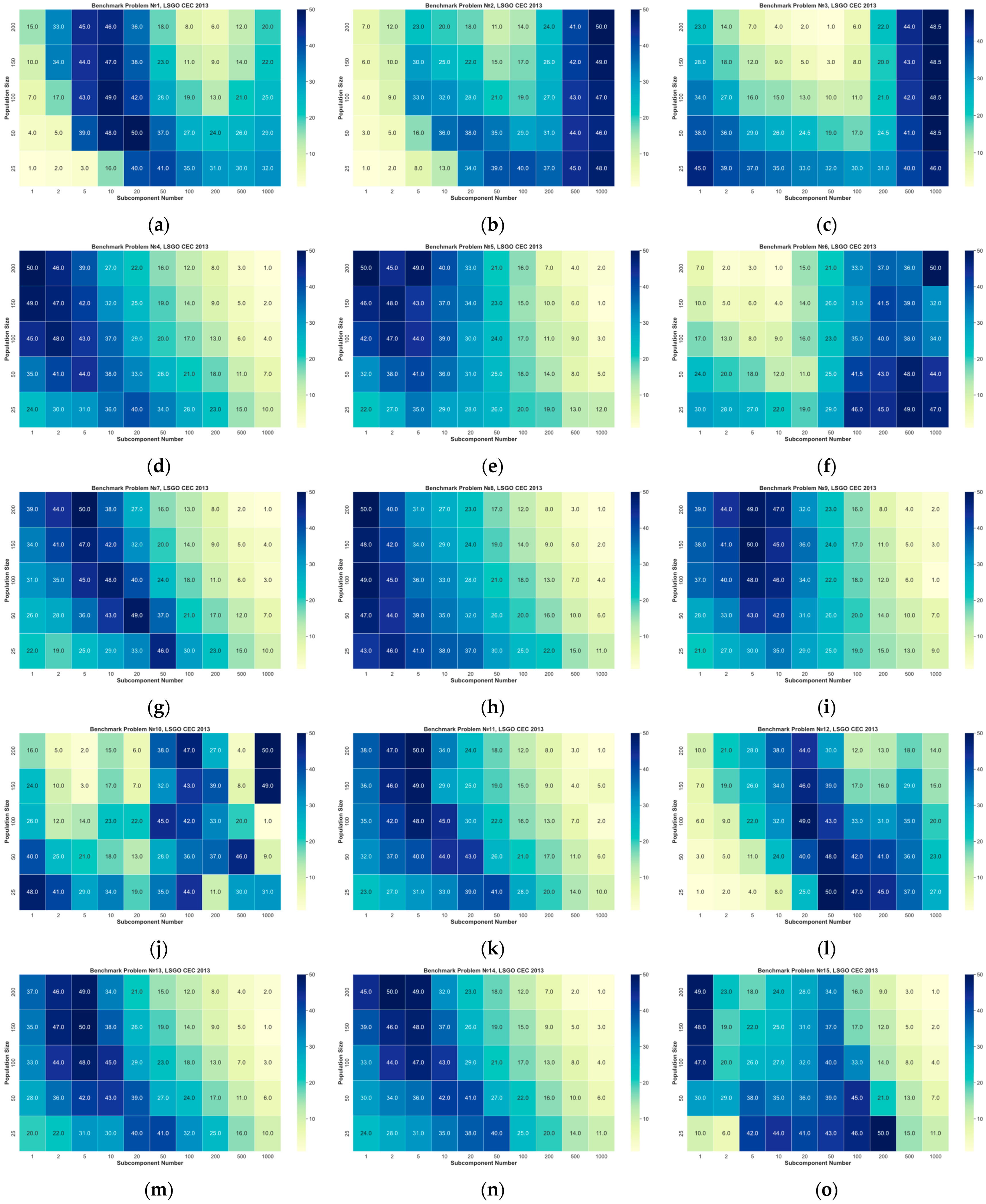
In this subsection we investigate the effect of CC-SHADE’s main parameters on its performance. The population size was set to 25, 50, 100, 150, and 200. The number of subcomponents was set to 1, 2, 5, 10, 20, 50, 100, 200, 500, and 1000. Figure 1 presents heatmaps for each benchmark problem and each combination of the parameters. The x-axis denotes the number of subcomponents, the y-axis denotes the population size. The total number of combinations is equal to 50 for each benchmark problem. The performance of each parameters’ combination is presented as a rank. The biggest number denotes the best average fitness value obtained in 25 independent runs. If two or more combinations of parameters have the same averaged fitness value, then their ranks are averaged. The ranks are colored in heatmaps from white (light) for the worst combination to dark blue (dark) for the best combination. The rank distributions are different in heatmaps for different optimization problems. 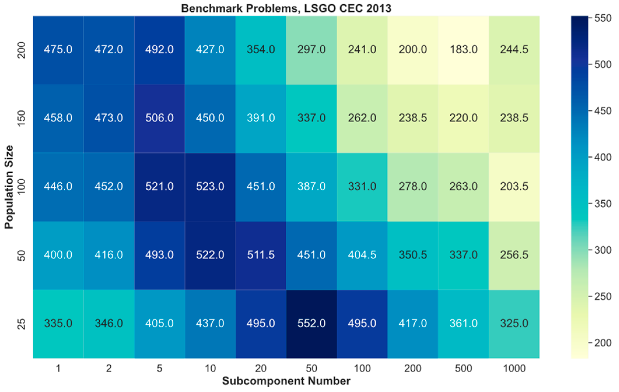Figure 2 shows the ranks sum for the algorithm’s parameters for all benchmark problems. The x-axis denotes the number of subcomponents, the y-axis denotes the number of individuals using the results from Figure 1. The highest sum of ranks is the best achieved result. Dark color denotes the best average combination of parameters. The best average combination of parameters for CC-SHADE are 50 subcomponents and 25 individuals.

Table 1. The best combination(s) of parameters for CC-SHADE on LSGO CEC’2013.

Benchmark Problem	The Best Combination(s)	Class
1	20 × 50	C1
2	1000 × 200	C1
3	1000 × 50, 1000 × 100, 1000 × 150, 1000 × 200	C1
4	1 × 200	C2
5	1 × 200	C2
6	1000 × 200	C2
7	5 × 200	C2
8	1 × 200	C3
9	5 × 150	C3
10	1000 × 200	C3
11	5 × 200	C3
12	50 × 25	C4
13	5 × 150	C4
14	2 × 200	C4
15	200 × 25	C5

shows the best combination(s) of parameters for each benchmark problem. The first column denotes the problem number, the second column denotes the best combination using the following notation, “CC × pop_size”, where CC is the best subcomponent size, and pop_size is the best population size. The last column denotes the class of a benchmark problem. As we can see from the results in Table 1, we cannot define the best combination of parameter combination for all problems. Additionally, we cannot find any pattern of the best parameters for each class of LSGO problems.

3.2. CC-SHADE-ML

We evaluated the performance of CC-SHADE-ML and compared it with CC-SHADE with a fixed number of subcomponents and a fixed number of individuals. The proposed CC-SHADE-ML algorithm has the following parameters. The set of subcomponents is equal to $\left\{1, 2, 5, 10, 20, 50, 100, 200, 500, 1000\right\}.$ The set of the population size is equal to $\left\{25, 50, 100, 150, 200\right\}$. The number of cycles is set to 50. According to our numerical experiments, this value for the number of cycles performs better than other tested values. Thus, in each cycle, CC-SHADE-ML evaluates 6.0 × 10⁴ FEs.

We use “CC” and “CC-k(v)” notations to save space in

Table 2. The Wilcox rank-sum test CC vs. CC-k(v).

CC vs.	CC-k(1)	CC-k(2)	CC-k(3)	CC-k(5)	CC-k(7)	CC-k(10)
+	215	215	193	218	185	190
-	417	421	439	423	448	452
≈	118	114	118	109	117	108

, where CC is all variants of CC-SHADE parameters, and CC-k(v) is the proposed approach, where the parameter k is set to v (3), and v is the power of the exponent in Equation (3). We investigated $v$ equal to $\left\{1, 2, 3, 5, 7, 10\right\}$. Table 2 proves the statistical difference in the results of the rank comparison using the Wilcoxon rank-sum test with the p-value equal to 0.05. The first column denotes better (+), worse (-), and equal performance (≈). Other columns contain the settings of the proposed algorithm. The cells contain the total number of benchmark problems where CC demonstrates better, worse, or equal performance in comparison with CC-k(v). As we can see, each version of the proposed algorithm has scores larger than CC. As we can see from Table 2, the proposed algorithm with all values of the power (3) always demonstrates better performance in comparison with the CC with a fixed number of subcomponents and individuals. Based on the results of the numerical experiments and the results of the statistical test, it is preferable on average to choose the proposed approach than the CC algorithm with an arbitrary set of parameters.

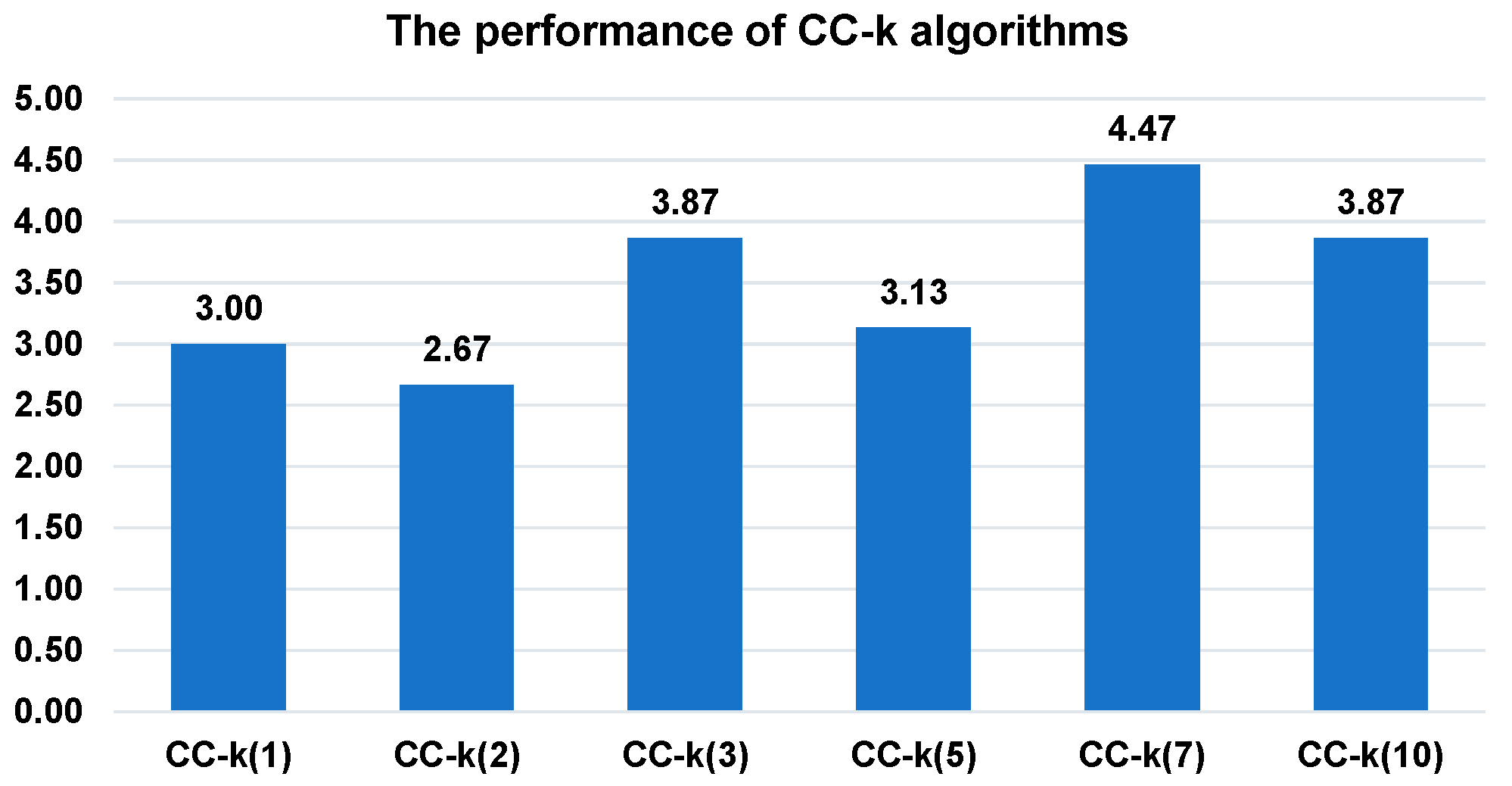
Figure 3 shows the ranking of CC-SHADE-ML algorithms with different values of power (3). The ranking is based on the obtained mean values in 25 independent runs. The ranking is averaged on 15 benchmark problems. The highest rank corresponds to the best algorithm.

We have compared the performance estimations of all CC-k algorithms. The statistical experimental results are placed in

Table 3. The results of the Wilcoxon test for CC-k with different parameter values.

Index	Algorithm	(2)	(3)	(4)	(5)	(6)
(1)	CC-k(1)	0/2/13	0/4/11	0/4/11	0/4/11	1/4/10
(2)	CC-k(2)	-	0/1/14	0/1/14	1/4/10	1/3/11
(3)	CC-k(3)	-	-	0/1/14	0/1/14	1/2/12
(4)	CC-k(5)	-	-	-	0/0/15	1/1/13
(5)	CC-k(7)	-	-	-	-	1/0/14
(6)	CC-k(10)	-	-	-	-	-

. The first column denotes indexes of the algorithm. The second column denotes the title of the algorithm. The next columns denote the compared algorithms corresponding to the index value. Values in each cell are based on the following notation. We compare algorithms from a row and column, if the algorithm from the row demonstrates statistically better, worse of equal performance we add points to the corresponding criterion. Table 3 contains the sum of (better/worse/equal) points of all algorithms.

The results in

Table 4. The sum of the Wilcoxon test results.

Number	Algorithm	Total Win	Total Loss	Total Equal	Averaged Rank
(5)	CC-k(7)	10	1	64	4.47
(6)	CC-k(10)	10	5	60	3.87
(3)	CC-k(3)	6	4	65	3.87
(4)	CC-k(5)	7	1	67	3.13
(2)	CC-k(2)	4	9	62	2.67
(1)	CC-k(1)	1	18	56	3.00

are based on the results from Table 3. Algorithms are sorted according to their statistical performance and their averaged rank. As we can see, CC-k(7) has taken first place. It outperforms the other algorithms 10 times, loses only once and demonstrates the same performance 64 times. It can be noted that the second last column contains large values. This means that the majority of considered algorithms demonstrate an equal performance on benchmark problems that can be explained by the introduced self-adaptiveness.

Based on the ranking and the statistical tests, we can conclude that CC-k(7) performs the other variants of CC-k(v). In the original paper [16], the authors also found that MLCC demonstrates better results with the power value (3) equal to 7.

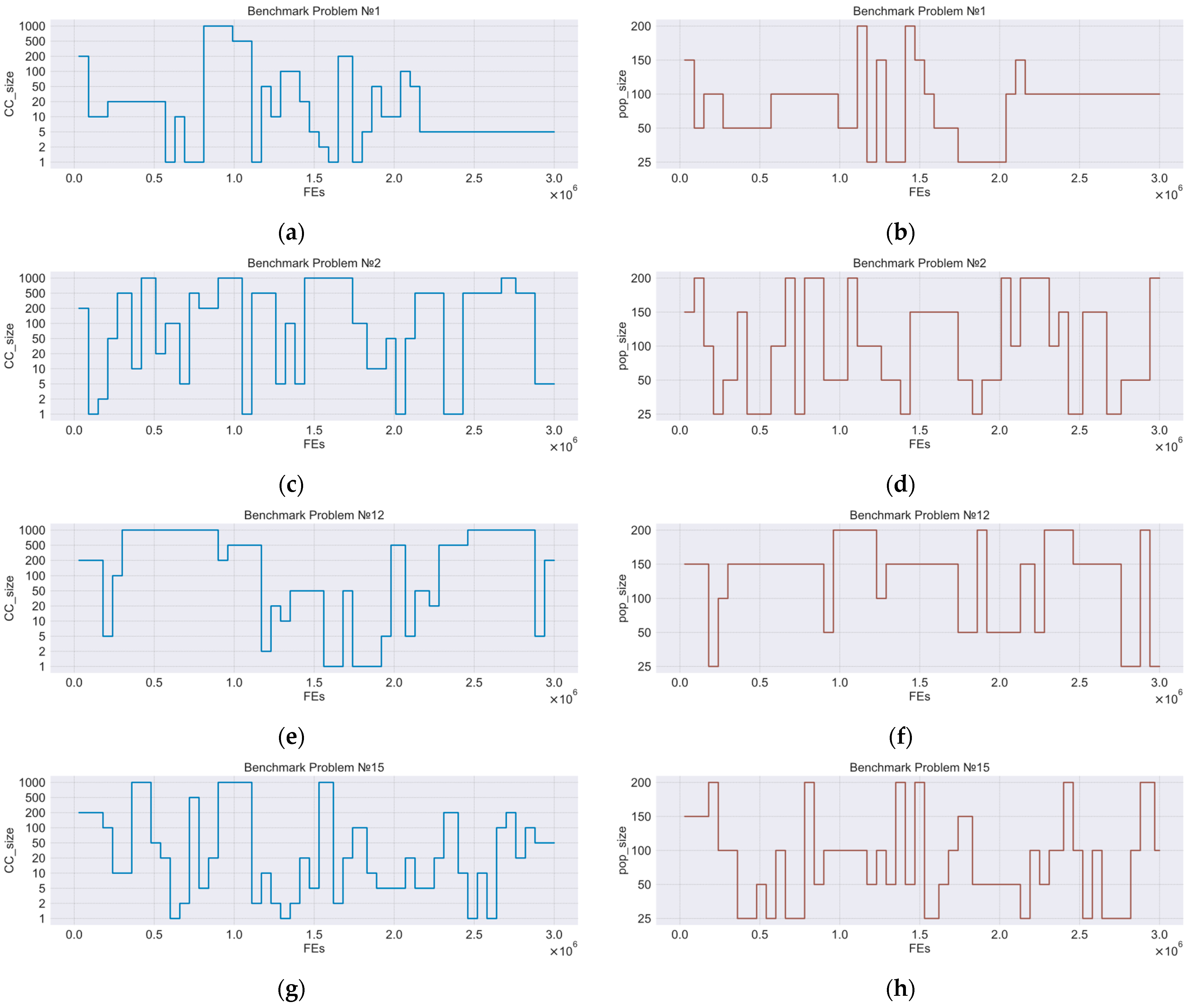
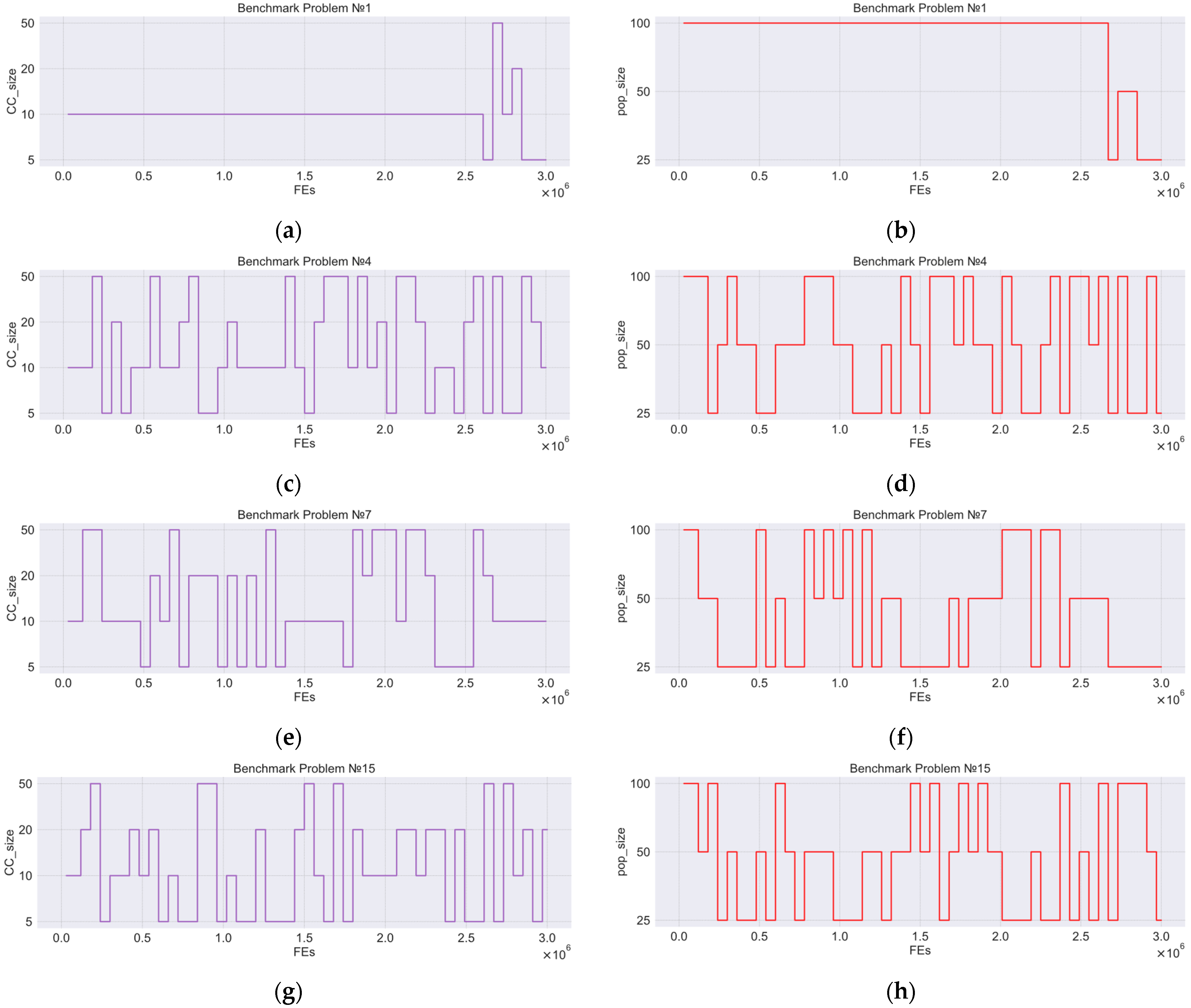
In Figure 4, we show an example of curves which demonstrate the dynamic adaptation of the number of subcomponents and the population size in one independent run of CC-k(7). The x-axis denotes the FEs, the y-axis denotes the selected level of parameters. The pictures show graphs for $F_1$, $F_2$, $F_{12}$, and $F_{15}$ benchmark problems.

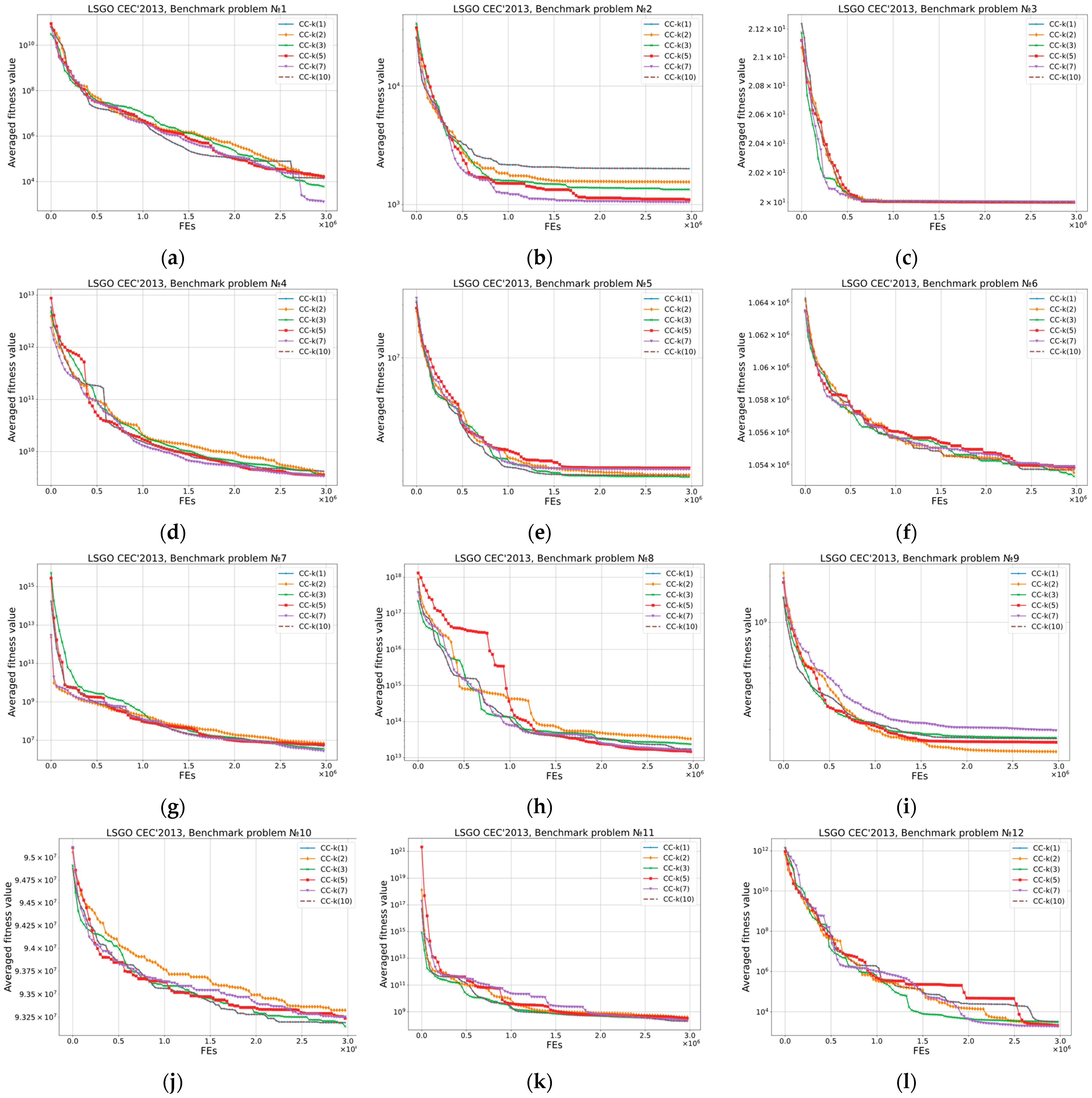
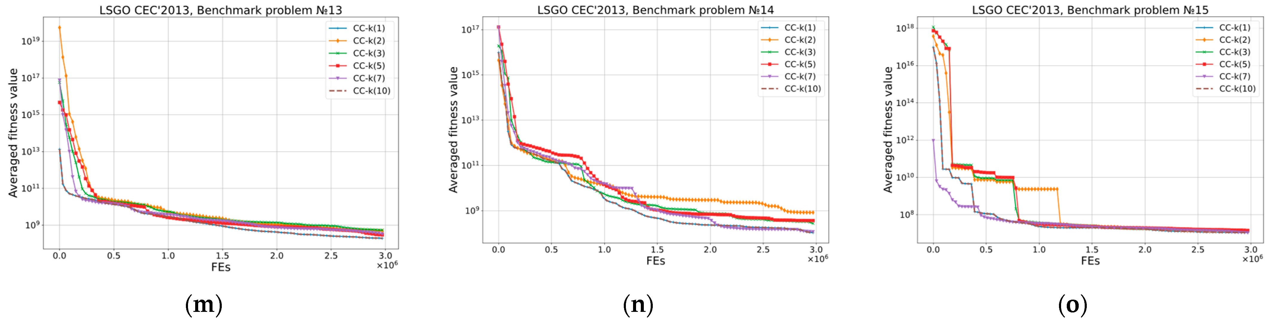
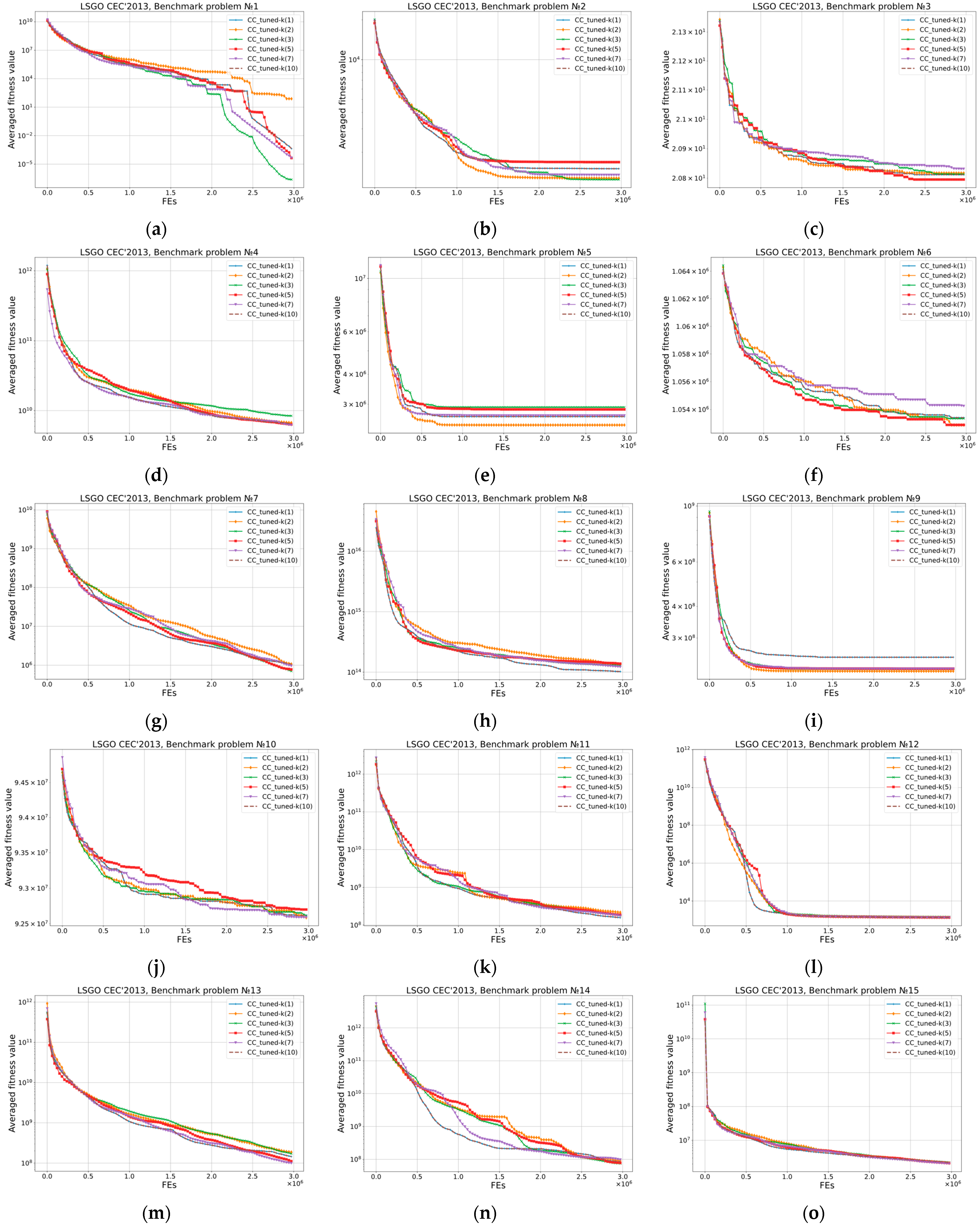
Figure 5 shows convergence graphs for CC-k(v) algorithms. The x-axis denotes the FEs number, the y-axis denotes the averaged fitness value obtained in 25 independent runs. As we can see, the convergence plots are almost similar for all CC-k algorithms. In most cases, the value of the power in (3) does not critically affect the behavior of the CC-SHADE-ML algorithm. As we have noted, according to the results from Table 4, the algorithms’ performance is the same on the majority of problems.

3.3. The Tuned CC-SHADE-ML

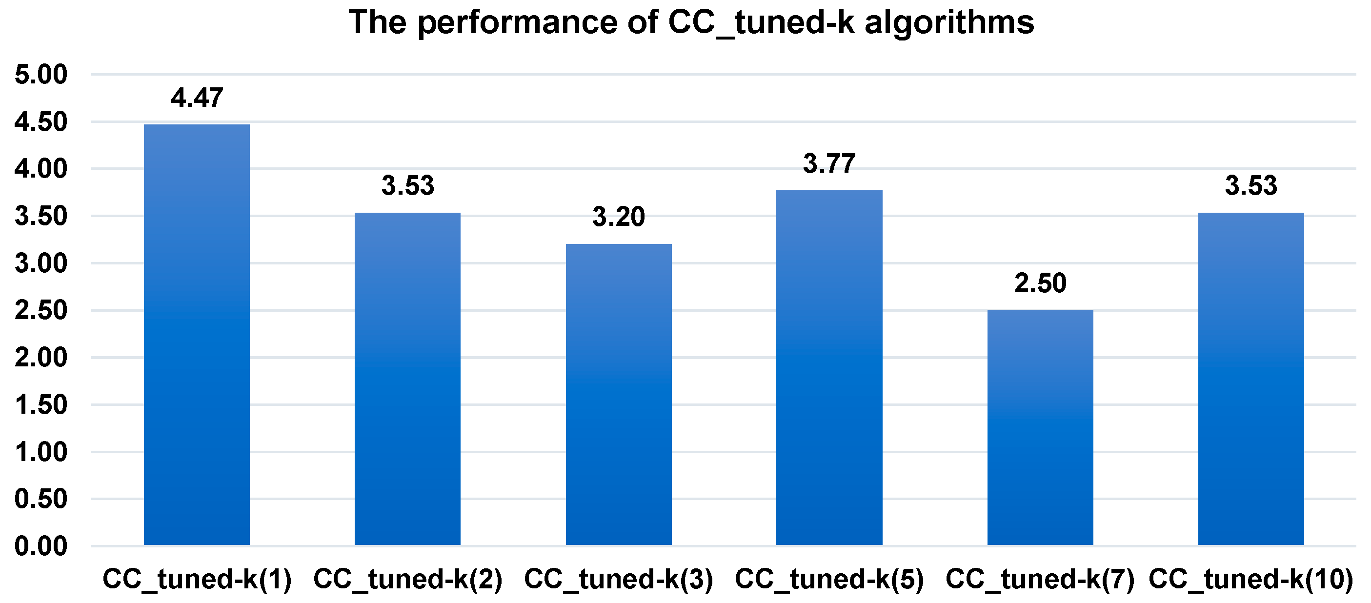
In this subsection, we evaluate the performance of the tuned CC-SHADE-ML. As we can see in Figure 2, the region with the best-ranked solutions covers the set of subcomponents equal to $\left\{5, 10, 20, 50\right\}$ and the set of the population size equal to $\left\{25, 50, 100\right\}$. The tuned CC-SHADE-ML will use these parameters. Figure 6 has the same structure as Figure 3. Based on the ranking, CC_tuned-k(1) demonstrates the best performance.

Table 5. The Wilcox rank-sum test CC vs. CC_tuned-k.

CC vs.	CC_tuned-k(1)	CC_tuned-k(2)	CC_tuned-k(3)	CC_tuned-k(5)	CC_tuned-k(7)	CC_tuned-k(10)
+	59	57	52	52	57	51
-	84	86	91	90	86	90
≈	37	37	37	38	37	39

has the same structure as Table 2. Table 2 compares the performance of CC and CC_tuned-k algorithms. According to the results of the Wilcoxon test, we can conclude that any power value of tuned CC-k demonstrates better performance than CC with the fixed number of subcomponents and individuals.

Table 6. The results of the Wilcoxon test for CC-k with different parameter values.

Number	Algorithm	(2)	(3)	(4)	(5)	(6)
(1)	CC_tuned-k(1)	0/0/15	0/1/14	0/1/14	0/1/14	0/1/14
(2)	CC_tuned-k(2)	-	0/2/13	0/0/15	0/2/13	0/1/14
(3)	CC_tuned-k(3)	-	-	2/1/12	0/1/14	1/0/14
(4)	CC_tuned-k(5)	-	-	-	0/0/15	0/0/15
(5)	CC_tuned-k(7)	-	-	-	-	1/0/14
(6)	CC_tuned-k(10)	-	-	-	-	-

and

Table 7. The sum of the Wilcoxon test results.

Number	Algorithm	Total Win	Total Loss	Total Equal	Averaged Rank
(5)	CC_tuned-k(7)	5	0	70	2.50
(3)	CC_tuned-k(3)	6	2	67	3.2
(6)	CC_tuned-k(10)	2	2	71	3.53
(4)	CC_tuned-k(5)	2	2	71	3.77
(1)	CC_tuned-k(1)	0	4	71	4.47
(2)	CC_tuned-k(2)	0	5	70	3.53

have the same structure as Table 3 and Table 4, respectively. We placed CC_tuned-k(7) on the first place because it has no loss point. Although, if we take into account only the averaged rank, we then need to place CC_tuned-k(7) in last place. Additionally, CC_tuned-k(1) has the highest rank, however, it does not significantly outperform any of compared algorithms.

We compared the performance of CC-k(7) and CC_tuned-k between each other using the Wilcoxon test. The statistical difference analysis is presented in

Table 8. The Wilcox rank-sum test CC-k(7) vs. CC_tuned-k(7).

CC-k(7) vs. CC_tuned-k(7)	F1	F2	F3	F4	F5	F6	F7	F8	F9	F10	F11	F12	F13	F14	F15
	-	+	+	+	≈	≈	-	+	≈	-	≈	-	≈	≈	-

. Columns denote the number of benchmark problems. The (+/-/≈) symbols mean better, worse, and equal performance of CC-k in comparison with CC_tuned-k. Algorithms demonstrate the same performance for six problems. CC-k outperforms CC_tuned-k on four problems and loses on five problems.

Figure 7 has the same structure as Figure 4. As we can see, on the F₁ benchmark problem, the algorithm has chosen a good combination of parameters and does not change the certain number of cycles because this combination demonstrates the high performance. On other benchmark problems, we can see more rapid switching between values of parameters. Figure 8 has the same structure as Figure 5. It shows convergence graphs for CC_tuned algorithms.

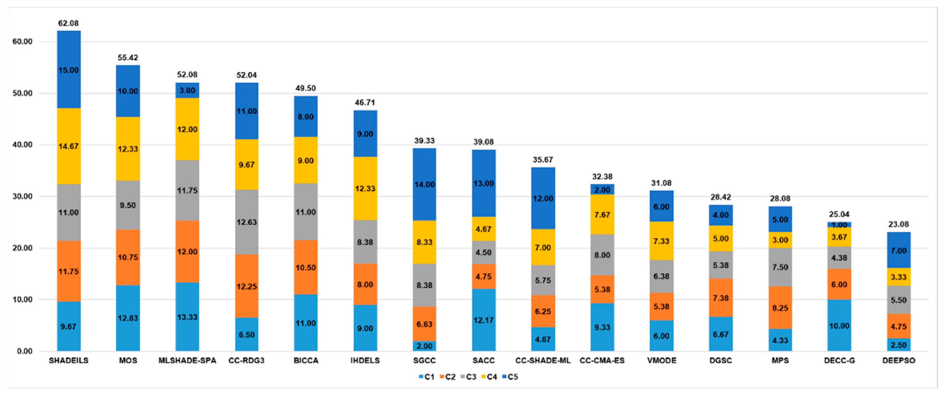
We have compared the performance of CC_tuned-k(7) with other state-of-the-art LSGO metaheuristics. These metaheuristics were specially created and tuned to solve the LSGO CEC’2013 benchmark set. We selected high-performed metaheuristics from the TACOlab database [26]: SHADEILS [27], MOS [28], MLSHADE-SPA [29], CC-RDG3 [30], BICCA [31], IHDELS [32], SGCC [33], SACC [34], CC-CMA-ES [35], VMODE [36], DGSC [37], MPS [38], DECC-G [39], and DEEPSO [40]. Figure 9 shows the ranking of the compared metaheuristics.

Table 9. The ranking of state-of-the-art metaheuristics.

Metaheuristic	C1	C2	C3	C4	C5	Total
SHADEILS	9.67	11.75	11.00	14.67	15.00	62.08
MOS	12.83	10.75	9.50	12.33	10.00	55.42
MLSHADE-SPA	13.33	12.00	11.75	12.00	3.00	52.08
CC-RDG3	6.50	12.25	12.63	9.67	11.00	52.04
BICCA	11.00	10.50	11.00	9.00	8.00	49.50
IHDELS	9.00	8.00	8.38	12.33	9.00	46.71
SGCC	2.00	6.63	8.38	8.33	14.00	39.33
SACC	12.17	4.75	4.50	4.67	13.00	39.08
CC-SHADE-ML	4.67	6.25	5.75	7.00	12.00	35.67
CC-CMA-ES	9.33	5.38	8.00	7.67	2.00	32.38
VMODE	6.00	5.38	6.38	7.33	6.00	31.08
DGSC	6.67	7.38	5.38	5.00	4.00	28.42
MPS	4.33	8.25	7.50	3.00	5.00	28.08
DECC-G	10.00	6.00	4.38	3.67	1.00	25.04
DEEPSO	2.50	4.75	5.50	3.33	7.00	23.08

consists of the ranking values of state-of-the-art algorithms depending on the class of benchmark problems. Ranks are averaged in each class. The proposed algorithm takes ninth place out of 15. We should note that the majority of metaheuristics in the comparison use special local search techniques adapted for the CEC’13 LSGO benchmark and their control parameters are also fine-tuned to the given problem set. Thus, there is no guarantee that these algorithms will demonstrate the same high performance with other LSGO problems. At the same time, the proposed approach automatically adapts to the given problem, so we conclude that it can also perform well when solving new LSGO problems. In Section 3.3, we propose a hybrid algorithm which is a combination of CC-SHADE-ML and MTS-LS1 [41].

Table 10. Detailed results for the fine-tuned CC-SHADE-ML algorithm.

		F1	F2	F3	F4	F5	F6	F7	F8
1.2 × 105	BEST	8.00 × 107	5.42 × 103	2.08 × 101	2.98 × 1010	2.83 × 106	1.05 × 106	4.36 × 108	4.37 × 1014
	MEADIAN	8.98 × 108	1.03 × 104	2.12 × 101	8.49 × 1010	5.50 × 106	1.06 × 106	1.84 × 109	3.58 × 1015
	WORST	4.51 × 109	1.29 × 104	2.13 × 101	4.80 × 1011	8.97 × 106	1.06 × 106	8.26 × 109	4.48 × 1016
	MEAN	1.58 × 109	9.94 × 103	2.11 × 101	1.13 × 1011	5.66 × 106	1.06 × 106	2.20 × 109	8.33 × 1015
	STD	1.49 × 109	1.93 × 103	1.35 × 10-1	9.03 × 1010	1.93 × 106	2.37 × 103	1.70 × 109	1.15 × 1016
6.0 × 105	BEST	1.79 × 103	1.28 × 103	2.08 × 101	9.30 × 109	1.47 × 106	1.05 × 106	9.95 × 106	9.78 × 1013
	MEADIAN	2.43 × 105	3.71 × 103	2.09 × 101	2.06 × 1010	2.53 × 106	1.06 × 106	4.74 × 107	3.02 × 1014
	WORST	1.28 × 107	5.97 × 103	2.11 × 101	4.91 × 1010	4.35 × 106	1.06 × 106	1.49 × 108	9.79 × 1014
	MEAN	1.80 × 106	3.64 × 103	2.09 × 101	2.25 × 1010	2.72 × 106	1.06 × 106	5.91 × 107	4.13 × 1014
	STD	3.64 × 106	1.45 × 103	9.31 × 10-2	1.01 × 1010	7.59 × 105	2.42 × 103	4.14 × 107	2.55 × 1014
3.0 × 106	BEST	2.32 × 10-23	8.16 × 102	2.07 × 101	1.06 × 109	1.47 × 106	1.05 × 106	7.09 × 104	4.10 × 1013
	MEADIAN	5.00 × 10-16	1.18 × 103	2.08 × 101	5.63 × 109	2.53 × 106	1.05 × 106	6.29 × 105	1.11 × 1014
	WORST	6.12 × 10-4	3.64 × 103	2.09 × 101	2.45 × 1010	4.18 × 106	1.06 × 106	2.99 × 106	2.63 × 1014
	MEAN	2.58 × 10-5	1.35 × 103	2.08 × 101	6.13 × 109	2.70 × 106	1.05 × 106	9.23 × 105	1.21 × 1014
	STD	1.22 × 10-4	5.73 × 102	3.91 × 10-2	4.68 × 109	7.29 × 105	2.25 × 103	8.83 × 105	5.46 × 1013
		F9	F10	F11	F12	F13	F14	F15
1.2 × 105	BEST	1.57 × 108	9.32 × 107	1.00 × 1010	1.96 × 108	1.04 × 1010	8.40 × 1010	1.46 × 107
	MEADIAN	4.11 × 108	9.42 × 107	1.05 × 1011	3.48 × 109	2.96 × 1010	5.19 × 1011	4.39 × 107
	WORST	1.15 × 109	9.48 × 107	3.98 × 1011	4.44 × 1010	9.13 × 1010	1.12 × 1012	2.46 × 108
	MEAN	4.28 × 108	9.42 × 107	1.44 × 1011	1.09 × 1010	4.13 × 1010	5.06 × 1011	5.90 × 107
	STD	2.09 × 108	3.67 × 105	1.25 × 1011	1.36 × 1010	2.59 × 1010	2.80 × 1011	5.16 × 107
6.0 × 105	BEST	9.45 × 107	9.21 × 107	6.49 × 108	1.46 × 103	1.15 × 109	4.10 × 108	4.76 × 106
	MEADIAN	2.07 × 108	9.33 × 107	2.15 × 109	5.92 × 103	2.81 × 109	2.44 × 109	1.01 × 107
	WORST	5.73 × 108	9.40 × 107	2.59 × 1010	2.42 × 106	6.60 × 109	1.28 × 1011	2.61 × 107
	MEAN	2.34 × 108	9.32 × 107	4.30 × 109	2.10 × 105	3.15 × 109	1.44 × 1010	1.22 × 107
	STD	1.13 × 108	3.85 × 105	6.43 × 109	6.60 × 105	1.43 × 109	2.74 × 1010	5.76 × 106
3.0 × 106	BEST	9.36 × 107	9.16 × 107	4.71 × 107	1.02 × 103	1.20 × 107	1.63 × 107	1.28 × 106
	MEADIAN	2.00 × 108	9.27 × 107	1.56 × 108	1.22 × 103	5.46 × 107	6.40 × 107	1.86 × 106
	WORST	5.74 × 108	9.31 × 107	3.53 × 108	1.99 × 103	4.66 × 108	5.42 × 108	3.14 × 106
	MEAN	2.27 × 108	9.26 × 107	1.71 × 108	1.32 × 103	9.75 × 107	9.41 × 107	2.00 × 106
	STD	1.12 × 108	3.44 × 105	9.20 × 107	2.89 × 102	1.19 × 108	1.11 × 108	5.73 × 105

contains the detailed results for the fine-tuned CC-SHADE-ML algorithm. The first column contains three checkpoints, 1.2 × 10⁵, 6.0 × 10⁵, and 3.0 × 10⁶. The remaining columns show the number of a benchmark problem. Each cell contains five numbers: the best-found value, the median value, the worst value, the mean value, and the standard deviation value. The authors of the LSGO CEC’2013 benchmark set recommend the inclusion of this information for the convenient further comparison of the proposed algorithm with others. Usually, the comparison is based on values after 3.0 × 10⁶ FEs.

3.4. Hybrid Algorithm Based on CC-SHADE-ML and MTS-LS1

In the CC-SHADE-ML algorithm, MTS-LS1 [41] performs after the optimization cycle and uses 25,000 FEs (this value has been defined by numerical experiments). MTS-LS1 tries to improve each i-th coordinate using the search range SR[i]. In this study, the initialization value of each SR[i] is equal to $\left(b_i-a_i\right)·0.4$. $a_i$ and $b_i$ are low and high bounds for the i-th variable. If MTS-LS1 does not improve a solution using the current value of SR[i], it should be reduced by two times (SR[i] = SR[i]/2). If SR[i] is less than 10⁻¹⁸ (in [41], the original threshold is 10⁻¹⁵), the value is reinitialized. As we can see from the numerical experiments, usually, MTS-LS1 finds a new best solution that is so far from other individuals in the population. Thus, CC-SHADE-ML is not able to improve the best-found solution after applying MTS-LS1, but it does improve the median fitness value in the population. In this case, Formula (2) will be inappropriate for the evaluation of the performance of selected parameters. We use Formula (4) to overcome this difficulty, the formula is based on the median fitness value before and after the CC-SHADE-ML cycle.

$$performanc{e}_i=\frac{medianFitnes{s}_{before}-medianFitnes{s}_{after}}{medianFitnes{s}_{before}}$$

(4)

Different mutation schemes have been evaluated and we determined that the best performance of CC-SHADE-ML-LS1 has been reached using the following Formula (5).

$$u_i=x_i+F_i\left(x_{pbest}-x_i\right)+F_i\left(x_t-x_r\right), i=1,\dots ,pop\_size$$

(5)

here, $u_i$ is a mutant vector, $x_i$ is a solution from the population, $F_i$ is a scale factor, $x_{pbest}$ is a solution from the population chosen from the p best solutions, $x_t$ is a solution from the population chosen using the tournament selection (in this study, the tournament size is equal to 2), $x_r$ is a randomly chosen solution from the population or from the archive. To perform Formula (5), the following condition must be met: $i\ne pbest\ne t\ne r$.

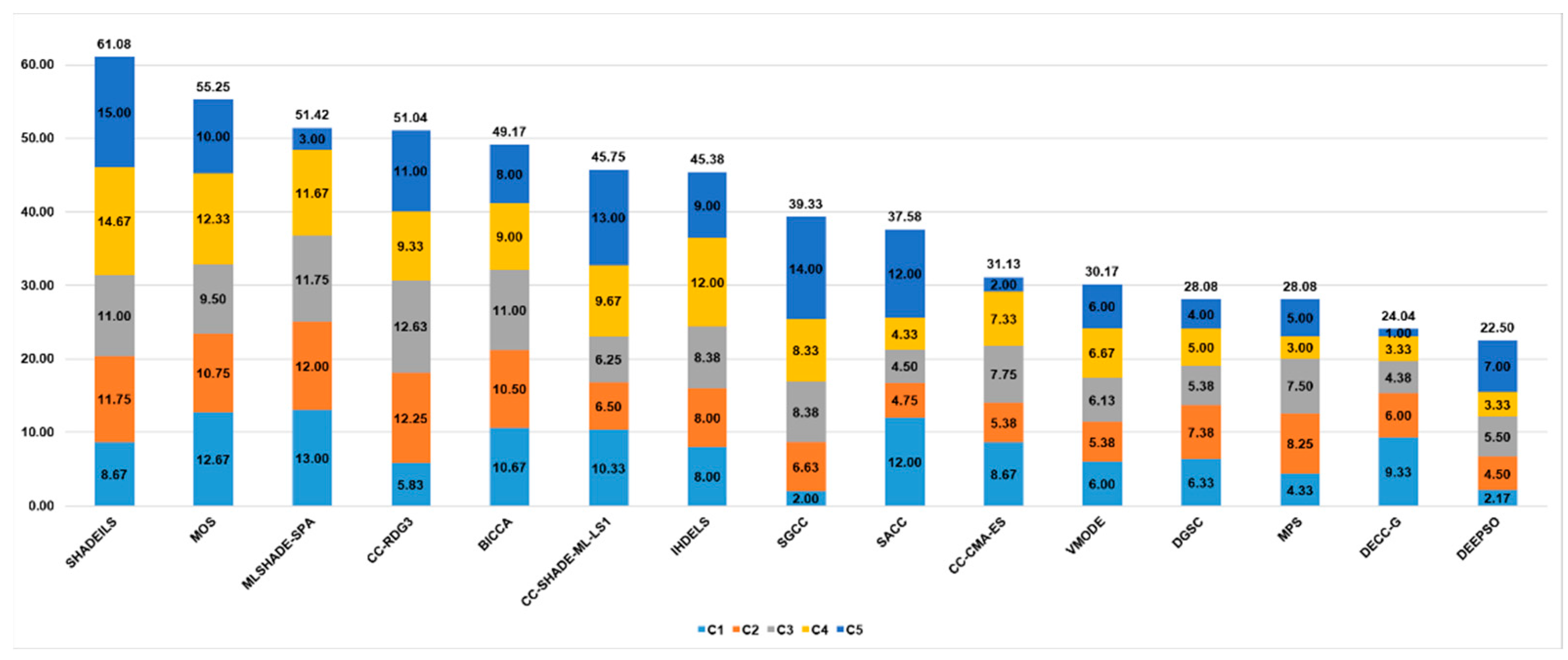
Control parameters of CC-SHADE-ML-LS1 are the following: the set of subcomponents equal to $\left\{5, 10, 20, 50\right\}$; the set of the population size equal to $\left\{25, 50, 100\right\}$; FEs_LS1 equal to 25,000; the mutation scheme, in SHADE, is (5); and the tournament size is 2. $\mathrm{FEs}\_\mathrm{cycle}\_\mathrm{init}$ is equal to 1.5 × 10⁵. The complete pseudocode of the hybrid is presented in Algorithm 3. Additionally, the CC-SHADE-ML-LS1 performance has been evaluated and compared with state-of-the-art metaheuristics. Comparison rules and algorithms for comparison are the same as in Section 3.2.

Table 11. The ranking of state-of-the-art metaheuristics.

Metaheuristic	C1	C2	C3	C4	C5	Total
SHADEILS	8.67	11.75	11.00	14.67	15.00	61.08
MOS	12.67	10.75	9.50	12.33	10.00	55.25
MLSHADE-SPA	13.00	12.00	11.75	11.67	3.00	51.42
CC-RDG3	5.83	12.25	12.63	9.33	11.00	51.04
BICCA	10.67	10.50	11.00	9.00	8.00	49.17
IHDELS	10.33	6.50	6.25	9.67	13.00	45.75
SGCC	8.00	8.00	8.38	12.00	9.00	45.38
SACC	2.00	6.63	8.38	8.33	14.00	39.33
CC-SHADE-ML-LS1	12.00	4.75	4.50	4.33	12.00	37.58
CC-CMA-ES	8.67	5.38	7.75	7.33	2.00	31.13
VMODE	6.00	5.38	6.13	6.67	6.00	30.17
DGSC	6.33	7.38	5.38	5.00	4.00	28.08
MPS	4.33	8.25	7.50	3.00	5.00	28.08
DECC-G	9.33	6.00	4.38	3.33	1.00	24.04
DEEPSO	2.17	4.50	5.50	3.33	7.00	22.50

and

Table 12. Detailed results for the fine-tuned CC-SHADE-ML-LS1 algorithm.

		F1	F2	F3	F4	F5	F6	F7	F8
1.2 × 105	BEST	3.91 × 103	5.94 × 103	2.11 × 101	6.35 × 1010	4.58 × 106	1.05 × 106	7.05 × 108	9.88 × 1014
	MEADIAN	5.49 × 103	8.47 × 103	2.12 × 101	1.92 × 1011	6.12 × 106	1.06 × 106	2.74 × 109	2.49 × 1015
	WORST	7.60 × 103	9.44 × 103	2.13 × 101	4.74 × 1011	7.28 × 106	1.06 × 106	4.78 × 109	3.05 × 1016
	MEAN	5.63 × 103	7.99 × 103	2.12 × 101	2.00 × 1011	6.12 × 106	1.06 × 106	2.52 × 109	6.75 × 1015
	STD	1.34 × 103	1.41 × 103	7.55 × 10-2	1.32 × 1011	1.04 × 106	3.06 × 103	1.31 × 109	1.06 × 1016
6.0 × 105	BEST	0.00 × 100	1.04 × 103	2.00 × 101	8.86 × 109	1.66 × 106	1.04 × 106	1.81 × 107	7.66 × 1013
	MEADIAN	0.00 × 100	1.18 × 103	2.00 × 101	3.92 × 1010	3.87 × 106	1.05 × 106	1.97 × 108	3.56 × 1014
	WORST	1.54 × 10-32	1.49 × 103	2.00 × 101	9.74 × 1010	5.59 × 106	1.05 × 106	6.84 × 108	2.14 × 1015
	MEAN	3.07 × 10-33	1.18 × 103	2.00 × 101	4.85 × 1010	3.61 × 106	1.05 × 106	2.33 × 108	5.32 × 1014
	STD	6.87 × 10-33	1.61 × 102	1.41 × 10-5	3.21 × 1010	1.58 × 106	3.16 × 103	2.54 × 108	7.21 × 1014
3.0 × 106	BEST	0.00 × 100	7.42 × 102	2.00 × 101	2.80 × 109	1.61 × 106	1.03 × 106	1.81 × 105	3.77 × 1013
	MEADIAN	0.00 × 100	7.77 × 102	2.00 × 101	3.11 × 109	3.87 × 106	1.04 × 106	5.17 × 105	6.87 × 1013
	WORST	0.00 × 100	1.33 × 103	2.00 × 101	9.54 × 109	5.05 × 106	1.05 × 106	7.00 × 105	1.11 × 1014
	MEAN	0.00 × 100	8.66 × 102	2.00 × 101	4.26 × 109	3.28 × 106	1.04 × 106	4.50 × 105	6.90 × 1013
	STD	0.00 × 100	2.07 × 102	1.41 × 10-5	2.47 × 109	1.28 × 106	7.18 × 103	2.23 × 105	2.87 × 1013
		F9	F10	F11	F12	F13	F14	F15
1.2 × 105	BEST	3.78 × 108	9.29 × 107	3.65 × 1010	3.63 × 108	1.47 × 1010	1.76 × 1011	2.96 × 107
	MEADIAN	4.56 × 108	9.39 × 107	1.86 × 1011	2.84 × 109	2.43 × 1010	2.51 × 1011	4.94 × 107
	WORST	8.71 × 108	9.46 × 107	4.39 × 1011	1.20 × 1010	7.16 × 1010	5.56 × 1011	7.50 × 107
	MEAN	5.07 × 108	9.38 × 107	2.27 × 1011	4.82 × 109	3.08 × 1010	2.77 × 1011	5.23 × 107
	STD	1.71 × 108	5.94 × 105	1.29 × 1011	5.26 × 109	1.89 × 1010	1.37 × 1011	1.59 × 107
6.0 × 105	BEST	1.58 × 108	9.26 × 107	1.39 × 109	5.84 × 102	1.21 × 109	3.21 × 109	5.66 × 106
	MEADIAN	3.78 × 108	9.30 × 107	4.54 × 109	8.54 × 102	3.49 × 109	3.18 × 1010	7.32 × 106
	WORST	4.22 × 108	9.40 × 107	5.82 × 1010	1.18 × 103	1.27 × 1010	7.89 × 1010	1.37 × 107
	MEAN	3.50 × 108	9.31 × 107	1.27 × 1010	9.08 × 102	4.57 × 109	3.50 × 1010	8.98 × 106
	STD	9.32 × 107	5.19 × 105	2.04 × 1010	2.19 × 102	3.98 × 109	2.99 × 1010	3.34 × 106
3.0 × 106	BEST	1.06 × 108	9.17 × 107	3.50 × 107	4.27 × 100	7.98 × 106	2.53 × 107	8.33 × 105
	MEADIAN	3.08 × 108	9.24 × 107	1.02 × 108	1.06 × 101	1.11 × 107	6.31 × 107	1.42 × 106
	WORST	3.58 × 108	9.26 × 107	3.95 × 108	1.06 × 103	6.14 × 107	1.56 × 108	2.56 × 106
	MEAN	2.60 × 108	9.23 × 107	1.50 × 108	2.84 × 102	2.35 × 107	7.11 × 107	1.55 × 106
	STD	1.04 × 108	3.23 × 105	1.29 × 108	4.22 × 102	2.19 × 107	4.58 × 107	6.65 × 105

have the same structure as Table 9 and Table 10, respectively. Table 11 shows the ranking of CC-SHADE-ML-LS1. Table 12 contains the detailed results of the tuned CC-SHADE-LS1 algorithm. Figure 10 has the same structure as Figure 9.

Algorithm 3 CC-SHADE-ML-LS1
Set the set of individuals, the set of subcomponents, optimizer, cycles_number
1:	Generate an initial population randomly;
2:	Initialize performance vectors, CC_performance and pop_performance;
3:	FEs_cycle_init = FEs_total/cycles_number;
4:	while (FEs_total > 0) do
5:	FEs_cycle = FEs_cycle_init;
6:	Randomly shuffle indices;
7:	Randomly select CC_size and pop_size from CC_performance and pop_performance;
8:	while (FEs_cycle > 0) do
9:	Find the median fitness value before the optimization cycle $medianFitnes{s}_{before}$;
10:	for i = 1 to CC_size
11:	Evaluate the i-th subcomponent using the SHADE algorithm;
12:	end for
13:	Find the median fitness value after the optimization cycle $medianFitnes{s}_{after}$;
14:	Evaluate performance of CC_size and pop_size using Equation (4);
15:	pdate CC_performance and pop_performance;
16:	end while
17:	while (FEs_LS1 > 0) do
18:	Apply MTS-LS1(best_fould_solution);
19:	end while
20:	end while
21:	return the best-found solution

4. Conclusions

In this paper, the CC-SHADE-ML algorithm has been proposed for solving large-scale global optimization problems. CC-SHADE-ML changes the number of subcomponents and the number of individuals according to their performance in the last cycles. The experimental results show that the proposed strategy can improve the performance of CC-based algorithms. We have investigated the proposed metaheuristic using the LSGO CEC’13 benchmark set with fifteen benchmark problems. The CC-SHADE-ML algorithm outperforms, on average, CC-SHADE algorithms with a fixed numbers of subcomponents and a fixed population size. All experiments are proven by the Wilcoxon test. CC-SHADE-ML has been compared with fourteen state-of-the-art metaheuristics. The numerical results indicate that the proposed CC-SHADE-ML algorithm is an efficient and competitive algorithm to tackle LSGO problems. We have also proposed hybridization of CC-SHADE-ML and MTS-LS1 algorithms. CC-SHADE-ML-LS1 has a high potential for enhancement. In our further works, we will improve the performance of the CC-SHADE-ML-LS1 algorithm by modifying the optimizer. Additionally, we will perform the comparison on a real-world LSGO problems for which the compared metaheuristics do not have fine-tuned control in order to prove the effect of self-configuration.