Article

A Novel Blind Restoration and Reconstruction Approach for CT Images Based on Sparse Representation and Hierarchical Bayesian-MAP

1
School of Information Engineering, Tianjin University of Commerce, Tianjin 300134, China
2
School of Electrical Automation and Information Engineering, Tianjin University, Tianjin 300072, China
*
Author to whom correspondence should be addressed.
Algorithms 2019, 12(8), 174; https://doi.org/10.3390/a12080174
Submission received: 29 May 2019 / Revised: 11 August 2019 / Accepted: 14 August 2019 / Published: 16 August 2019
(This article belongs to the Special Issue The Second Symposium on Machine Intelligence and Data Analytics)

Abstract

:
Computed tomography (CT) image reconstruction and restoration are very important in medical image processing, and are associated together to be an inverse problem. Image iterative reconstruction is a key tool to increase the applicability of CT imaging and reduce radiation dose. Nevertheless, traditional image iterative reconstruction methods are limited by the sampling theorem and also the blurring of projection data will propagate unhampered artifact in the reconstructed image. To overcome these problems, image restoration techniques should be developed to accurately correct a wide variety of image degrading effects in order to effectively improve image reconstruction. In this paper, a blind image restoration technique is embedded in the compressive sensing CT image reconstruction, which can result in a high-quality reconstruction image using fewer projection data. Because a small amount of data can be obtained by radiation in a shorter time, high-quality image reconstruction with less data is equivalent to reducing radiation dose. Technically, both the blurring process and the sparse representation of the sharp CT image are first modeled as a serial of parameters. The sharp CT image will be obtained from the estimated sparse representation. Then, the model parameters are estimated by a hierarchical Bayesian maximum posteriori formulation. Finally, the estimated model parameters are optimized to obtain the final image reconstruction. We demonstrate the effectiveness of the proposed method with the simulation experiments in terms of the peak signal to noise ratio (PSNR), and structural similarity index (SSIM).

1. Introduction

CT (computed tomography) images are widely used in clinical diagnosis [1]. However, radiation exposure and the associated risk of cancer for patients in CT scans have already been one of the focusing concerns for medical and scientific research. To reduce radiation dose in CT scans, the iterative reconstruction methods were concerned in CT reconstruction because the iterative reconstruction methods can reconstruct CT images with few numbers of measured projection. Furthermore, the fewer numbers of measured projection can be acquired by fast scanning, and thus, the radiation dose delivered to the patients can be decreased [2]. SART (simultaneous algebraic reconstruction technique) is an iterative image reconstruction method [3] and plays a significant role in the quality of CT image reconstruction. However, the SART reconstruction method is limited by Nyquist sampling theorem [4], and CT images cannot be reconstructed by the measured projection data that does not satisfy sampling conditions. To further reduce radiation dose and perform CT image reconstruction with fewer measured projection data, the compressed sensing (CS) theory has been used recently. Compressive sensing (CS) converts the images, embedded in a high dimensional space, into a sparse representation that lie in the space of significantly smaller dimensions [5]. Sparse representations can be obtained with fewer data. Then, the reconstructed image is obtained by sparse representation. Compressive sensing theory guarantees that CT image reconstruction can be implemented by fewer measured projection that does not satisfy the sampling theorem [6,7,8,9,10].
On the other hand, it is apparent that the measured projection data has been degraded not only by noise but also by a point spread function [11]. The degradation of the measured projection data will propagate unhampered artifact in reconstructed images. Nevertheless, in the case of fewer projection data or serious degradation, SART reconstruction will be ineffective or seriously affect the result of the diagnosis. Image restoration method, a mechanism for eliminating the influence of the point spread function, was inserted into the iterative CT image reconstruction technique to form an optimization problem [12]. This method is appropriate in certain settings when the point spread function is known, and the measured noisy projection data satisfies the Nyquist sampling theorem. As a rapidly developing iterative algorithm, the CS reconstruction algorithm can complete CT reconstruction with fewer data. TV (total variation) transform [13], and wavelet transform [14] are the two most commonly used sparse representation methods. However, these CS algorithms have not considered for the point spread function, and the degradation caused by the point spread function can seriously affect the quality of the reconstruction image. Blind image restoration [15,16] is a method that estimates images and eliminates the influence of the point spread function when the point spread function is unknown. To solve the CT reconstruction problem based on CS when the point spread function is unknown, a blind image restoration technique was embedded into the iterative process of compressive sensing CT image reconstruction. At each iteration, the iterative output image is improved because blind image restoration is introduced into the algorithm. Correspondingly, the input of the next iteration will be improved, and the convergence of the whole algorithm will be accelerated.
CT reconstruction problem based on CS with blind image restoration is an ill-posed problem [17]. Bayesian methods were used to solve the ill-posed problem. Bayesian methods can provide a variety of probability distribution prediction to estimate the parameters, which can achieve the estimation of uncertainties in the CT blind restoration reconstruction with good anti-noise performance. The probability distributions are adopted as regularization terms to constrain the solution space. The constrained solution space can accelerate the convergence of the algorithm and obtain a reliable solution. Some prior distributions for some parameters were widely used as the regularization terms, such as total-variation (TV) priors [18], Student-t priors [19], Laplacian priors [20]. The stronger the sparse prior knowledge is, the better the image reconstruction ability is. TV prior is often used in CT image reconstruction [13]; however, TV prior causes over smoothing or blocky artifacts in the reconstructed images. Therefore, a compound Gaussian distribution and a multivariate Gaussian distribution can be chosen as priors for modeling two unknown parameters, the sparse representation and the point spread function, respectively. In this paper, we utilized a hierarchical Bayesian Maximum-a-Posteriori (MAP) formulation to estimate the sparse representation and the point spread function, respectively. The hierarchical Bayesian-MAP formulation is a statistical model written in multiple levels that can estimate the parameters of the posterior distribution using the Bayesian-MAP method [21]. The hierarchical model for the inverse problem was introduced into the problem of CT image reconstruction with blind image restoration in this paper. The problem of CT reconstruction with the blind restoration was transformed into the estimation of some specific parameters. All of the parameters were estimated by the hierarchical Bayesian MAP. Experiments simulate the fewer data environment by sampling complete projection data.
This paper is organized as follows. Section 2 presents the basic problem of medical CT image blind restoration and reconstruction with different parameters and derives the stochastic hierarchical Bayesian maximum for solving the medical CT image reconstruction with blind restoration and presents a proposed algorithm. Section 3 reports the experimental results of applying the proposed algorithm to medical CT image blind restoration. Section 4 concludes this paper.

2. Materials and Methods

2.1. CT Image Blind Restoration and Reconstruction

A standard formulation of the CT image blind restoration and reconstruction is given in the following vector-matrix form:
P = A H ψ α + n
where P m × 1 is the known noisy projection data; A m × m is the known measurement matrix of the X-ray CT system; H m × m is the unknown blurring matrix constructed by the point spread function ( h m × 1 denotes the point spread function (PSF) in vector form, H performs convolution with h ); ψ m × k ( k < < m ) is a sparse representation transform matrix and is known. f denotes the CT image. f m × 1 can be changed into another form α k × 1 by the sparse representation transform matrix, f = ψ α . α denotes the sparse representation vector because it can describe the image and include fewer data. n m × 1 is the additive noise vector, n ~ N ( 0 ,   n ) , n m × m is the covariance matrix. For simplicity, we assume that n = σ n 2 I . The problem in (1) is designed to estimate α and H when the projection data P is as few as possible. Here, α is for the estimation of CT image. It doesn’t matter what is H itself. The purpose of estimating H is to eliminate the degradation caused by PSF.
As to estimate α k × 1 with the assumption, the problem is to solve the following problem
α ^ = arg max α log p ( α | P )
By applying the Bayesian formula, p ( x | y ) = p ( y | x ) p ( x ) p ( y ) , (2) can be written as
α ^ = arg max α { log p ( P | α ) + log p ( α ) }
where p ( α ) is the prior probability distribution of α . p ( α ) provides the prior statistical information of the sparse representation. The closer the estimated prior distribution is to the actual distribution, the more accurate the estimated value of α will be. To this end, the statistical prior of α was described by a Gaussian compound distribution as did in [22]. In this case, the probability density is given by
p ( α ) = 0 + 1 ( 2 π ) k 2 | z 2 v | 1 2 exp ( α T v 1 α 2 z 2 ) ϕ z ( z ) d z
where the mixing variable z 0 is a random vector, z k × 1 . ϕ z ( z ) defines the probability density of the scale variable and results in the different distribution in different applications.
The Gaussian compound distribution α is not easy to solve directly, and the hierarchical Bayesian strategy is applied to convert α into the synthesis of two variables with the following form.
α = z V
where defines the Hadamard product. V ~ N ( 0 ,   v ) denotes a Gaussian random vector, V k × 1 . v k × k is the covariance matrix of V . For the sake of simplicity, we assume that z and V are independent. Therefore, (1) results in
P = A H ψ ( z V ) + n
To solve the problem conveniently, the mixing variable z can be described by a Gaussian variable x k × 1 and a nonlinear function g ( ) [21], z = g ( x ) . When g ( x ) is chosen as a candidate for z , optimizing z is equal to optimizing x . (6) results in
P = A H ψ ( g ( x ) V ) + n
We choose g ( x ) as a non-linear function with the following form,
g ( x ) = exp ( x / β )
where β is a controlling scale factor.
A compound Gaussian distribution can be used to fit an unknown variable by the combination of the known distributions of two variables. As can be seen from (7), if H is known, the estimates of variables x and V can be obtained by iteration as shown below, and then α can be obtained by (5). Therefore, the hierarchical Bayesian MAP is designed to estimate x , V and H , respectively. In previous methods, H is generally assumed to be the identity matrix. In other words, the effect of point spread function is not considered. We will develop a new approach to approximate H in the next section.

2.2. The Hierarchical Bayesian MAP

The hierarchical Bayesian MAP is a statistical model written in multiple levels that estimates the parameters of the posterior distribution using the MAP method. The estimation of the sparse representation α can be decomposed into the estimation of two independent parameters x and V as shown in (7).
x ^ = arg max x P T M 1 ( x ) P + log det M ( x ) + x T x 1 x
where, det ( M ( x ) ) is the determinant of M ( x ) and
M ( x ) = A H ψ G ( x ) v G ( x ) ψ T H T A T + n , M ( x ) m × m
G ( x ) = d i a g ( g ( x ) ) k × k
where d i a g ( ) is a square diagonal. Assuming that x is known, we can obtain the following solution by using the Bayesian formula
V ^ = arg max V { log p ( P | V ) + log p ( V ) }
Substituting (7) and (9) into (12), the following solution can be obtained
V ^ = arg max V ( P A H ψ G ( x ^ ) V ) T n 1 ( P A H ψ G ( x ^ ) V ) + V T v 1 V
(12) is quadratic on the unknown variable V and its solution is given,
V ^ = ( ( G T ( x ^ ) ψ T H T A T ) n 1 ( A H ψ G ( x ^ ) ) + v 1 ) 1 ( A H ψ G ( x ^ ) ) T P
According to (7) and (14), the estimation of the sharp CT image is given by f ^ = ψ α ^ = ψ ( z ^ V ^ ) .
In (9) and (14), the blurring matrix H is usually unknown, so the degradation matrix H must be estimated. Generally, H is a circular matrix, and it can be obtained by a cyclic shift of any row h j , ( j = 1 , 2 , , m ) . Therefore, we can obtain the blurring matrix H by estimating the point spread function. Here, the Fourier transform was implemented before we estimate h , h ˜ and h ˜ 0 are the Fourier transform of h and h 0 , respectively. h 0 is an initial estimation of h . A multivariate Gaussian distribution is chosen for the prior of the point spread function h ˜ [23].
p ( h ˜ ) = 1 ( 2 π ) m 2 | Σ h | 1 2 exp ( 1 2 ( h ˜ h ˜ 0 ) T Σ h ˜ 1 ( h ˜ h ˜ 0 ) )
where Σ h ˜ is the covariance matrix of the variable h ˜ . Next, we solve h ˜ in Fourier domain,
p ( P ˜ | f ˜ , Σ n , h ˜ ) = 1 ( 2 π ) m 2 | Σ n | 1 2 exp ( 1 2 ( P ˜ Σ A f h ˜ ) T Σ n 1 ( P ˜ Σ A f h ˜ ) )
where y = A f m × 1 , y ˜ is the Fourier transform of y with Σ A f = diag ( y ˜ ) . By calculating by (15) and (16), the conditional distribution h ˜ is followed as
p ( h ˜ | f ˜ , P ˜ , Σ n ) exp ( 1 2 ( P ˜ Σ A f h ˜ ) T Σ n 1 ( P ˜ Σ A f h ˜ ) ) exp ( 1 2 ( h ˜ h ˜ 0 ) T Σ h 1 ( h ˜ h ˜ 0 ) )
According to (17), the conditional distribution h ˜ can be described by a multivariate Gaussian distribution. For simplicity, we assume that n = σ n 2 I . Since H is circular, it holds Σ h = σ h 2 I . The mean vector and covariance matrix of the multivariate Gaussian distribution is given respectively,
m ˜ = ( Ι σ h 2 + | Σ A f | 2 σ n 2 ) 1 ( h ˜ 0 σ h 2 + Σ A f T P ˜ σ n 2 )
C ˜ = Ι σ h 2 + | Σ A f | 2 σ n 2
The multivariate Gaussian distribution is easy to sample, and the conditional distribution h ˜ can be obtained. The inverse Fourier transform of the conditional distribution of h ˜ was implemented to obtain the point spread function h . Furthermore, the cyclic shift h was implemented to obtain the degradation matrix H . The proposed algorithm is described in the Table 1.
To reconstruct CT image with far fewer projection data, a compressed sensing image reconstruction algorithm including a blind image restoration process was proposed. Image reconstruction is achieved by estimating a sparse coefficient vector. We utilized the hierarchical Bayesian model and transformed the image estimation into two independent variables estimation. The hierarchical Bayesian MAP method solved the problem of parameter estimation. The introduction of blind image restoration mechanism improves the quality of the output image in each iteration and improves the quality of the final reconstructed image. Therefore, under the same image quality requirements, the proposed method can effectively reduce the radiation dose.

3. Results

In the experiments, four true CT images and simulated projections were used to study the performance of our algorithm under degraded conditions. The experimental setting is as follows: The image size is set to be 512 × 512. The known projection data are obtained by convolution of the CT system matrix A and the true CT image. The size of the CT system matrix is different according to different image sizes. The system matrix of the fan beam scanning mode [25] is used in the experiment. The point spread function of the CT image is approximated as a standard Gauss function process with different sizes, 20 × 20, 27 × 27, 18 × 18, 15 × 15, respectively and the same variance, σ 2 = 1 . The white Gaussian noise is added to the known projection data to obtain the known noisy projection data with signal-to-noise ratio (SNR) 20 dB and 40 dB. All known measurement projection data is acquired through binary matrices to verify the applicability of the method. The sampling ratio varies from 40%–100%. To simulate fewer data and make a comparative analysis, a few data were obtained by random sampling of complete data. The sampling ratio rate represents the amount of sample data. The lower the sampling rate, the fewer the data used in the experiment. In other words, fewer data represent lower radiation doses. One can initialize the point spread function to a Dirac delta function. ψ is a sparse representation matrix and represents wavelet sparse transform in this paper [14]. Here the Haar basis was chosen as wavelet transformation basis.
The stopping criterion of the iteration is accomplished by relative error. That is h ( l + 1 ) h ( l ) / h ( l ) t o l and t o l is a relatively small constant. In the simulation experiment, t o l = 10 6 .
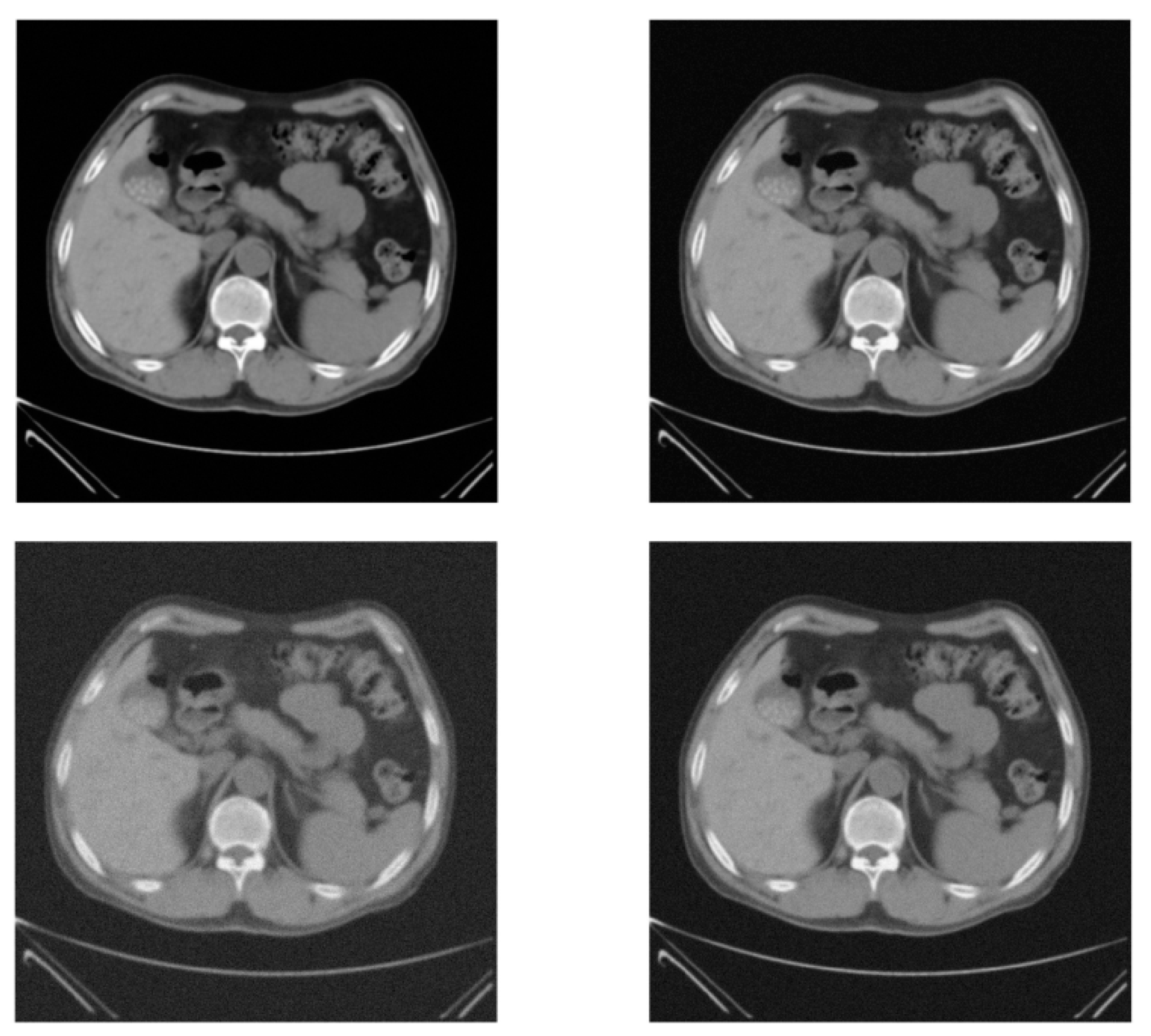
When the relative error is less than t o l , the algorithm terminates. Figure 1, Figure 2, Figure 3 and Figure 4 present CT image blind restoration and reconstruction results using the proposed approach for four different images degraded with different Gaussian PSF. Good results were obtained in terms of clarity contrast, detail retention, and so on. Although the image quality decreases with the decrease in the sampling ratio, it is acceptable in general.
From Figure 1, Figure 2, Figure 3 and Figure 4, it is clear that the proposed algorithm has good reconstruction performance in the case of high sampling ratio. With the decrease of sampling ratio, the image quality also decreases. Moreover, until a lower sampling ratio of 0.4, an intuitive and acceptable image can be reconstructed for medical diagnosis services. In the case of high signal-to-noise ratio, the proposed method can obtain better reconstruction results at a sampling rate of 40%. Other methods cannot achieve good reconstruction at this sampling rate. With the decrease of the signal-to-noise ratio, the reconstruction results can be obtained at the sampling rate of 40%, but the quality will decrease significantly. The reconstruction results of the other three methods can be obtained in the Supplementary Materials.
For quantitative comparison, the peak signal-to-noise ratio (PSNR) and structural similarity index metric (SSIM) are used to evaluate the algorithm performance at SNR = 40 dB. About these two metrics, the ideal value of PSNR is +∞, the ideal values of SSIM are 1. These two metrics can only be used in the simulated experiments because they require a referred image. The above two metrics tabulated for each experiment are the average values over 10 times repetitions. The results are shown in Table 2 and Table 3. The reported values are the average and standard deviation of the 10 runs. The less standard deviation judges the robustness of the proposed approach method. Because the compound Gaussian distribution provides better prior information, the reconstruction method based on hierarchical Bayesian structure has better performance in the case of high sampling rate.
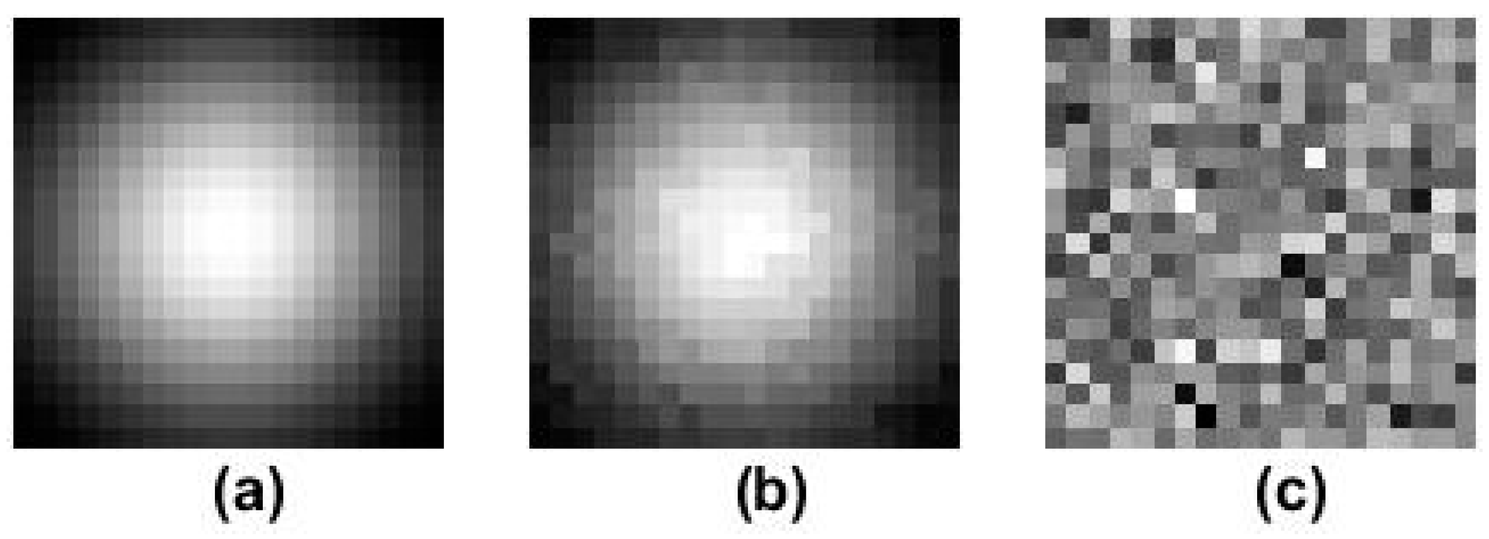
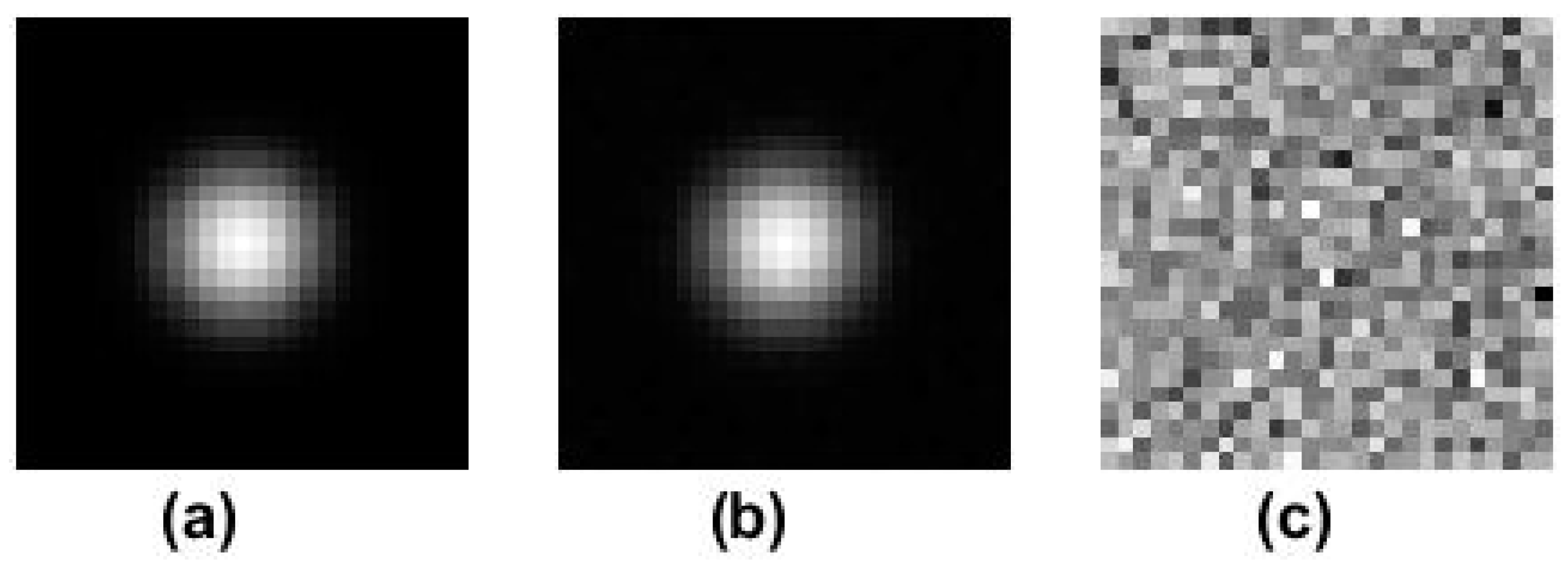
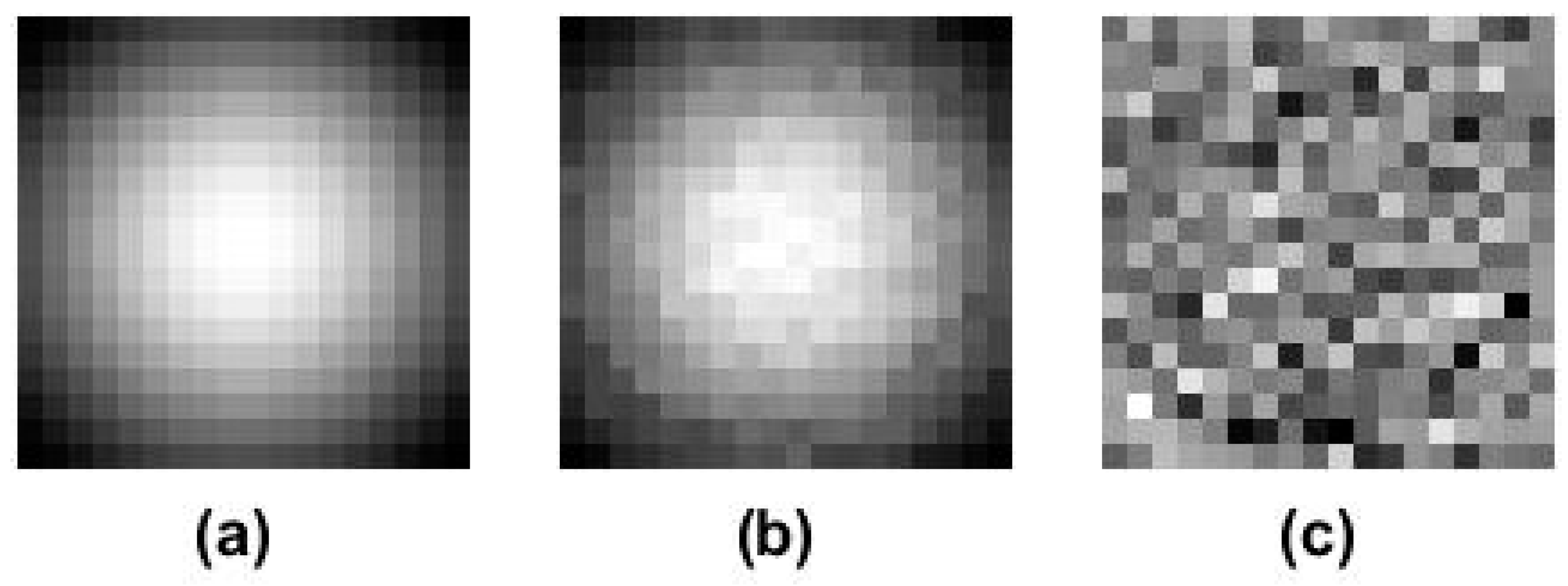
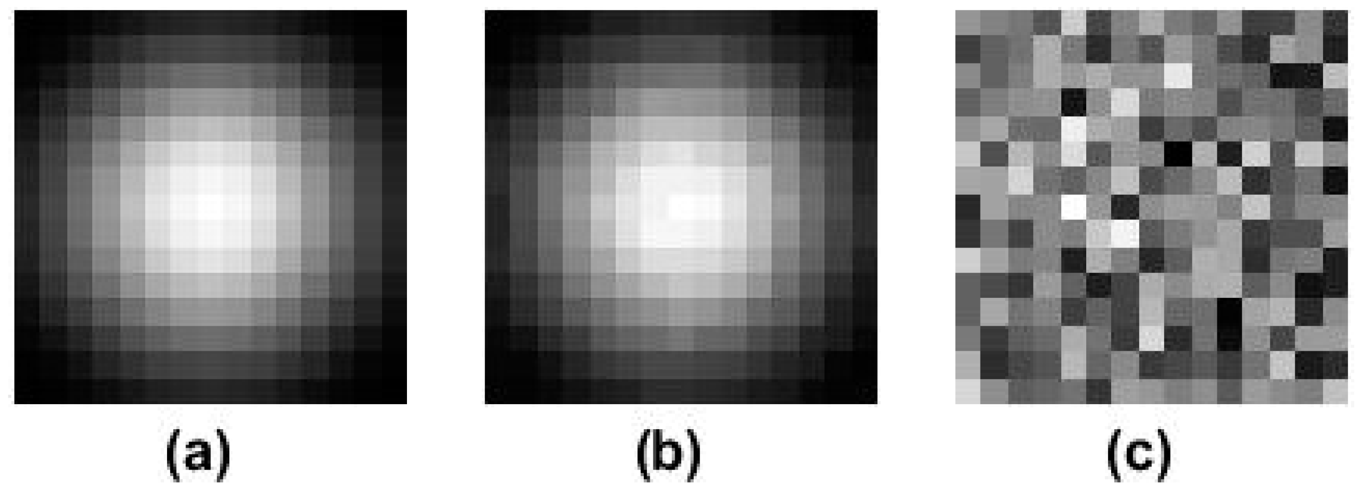
Figure 5, Figure 6, Figure 7 and Figure 8 depict the estimated point spread function and compare it to the ground-truth simulated one. The results show that a better estimation can be obtained. As a result of the better estimation of PSF, the better reconstructed image can be obtained, as shown in Figure 1, Figure 2, Figure 3 and Figure 4. Performance evaluation is shown in Table 2 and Table 3.
Table 2 presents an average performance comparison of the proposed approach with a set of image reconstruction algorithms. SART [3] is a popular iterative image reconstruction method, and it is effective in the case of high compressive sensing ratio. The other two methods are TV transform [13] and wavelet transform [14]. The above average performance for four methods are the average values over 10 times repetitions. They are suitable for low sampling ratio. Therefore, when the influence of point spread function exists, the performance of the three methods can be compared.
As shown in Table 3, the structural similarity index is improved compared to the traditional methods. All kinds of objective image quality metrics have been improved in different compressive sensing ratio. In the case of very low sampling ratio, other algorithms cannot reconstruct images, but the proposed algorithm can achieve relatively good performance. Of course, the quality of the reconstructed image at low sampling ratio has decreased compared with that at high sampling ratio. SSIM is a full reference metric that requires two images from the same image capture—a reference image and a processed image. It actually measures the perceptual difference between two similar images. It cannot judge which of the two is better. In other words, the closer the reconstructed image is to the real image, the better the reconstructed image is.
The proposed method shows acceptable performance for sampling ratio greater than 0.4 and exhibits similar fluctuations over increasing sampling ratio. On the other hand, other algorithms have relatively good performance over high ratios. However, when the ratio is less than or equal to 0.4, the image performance is unacceptable. The lower sampling ratio is, the fewer data used for image reconstruction is. The fewer data for reconstructed images means less radiation dose for patients. Experiments show that the proposed method can reduce the radiation impact on patients under the same image quality requirements. Compared with the other three methods, the proposed method consumes more computing time due to multi-parameter hierarchical iteration. In the future research, improving the computational efficiency is the further research content.
Figure 9 and Table 4 present CT image blind restoration and reconstruction results using the proposed approach and a reconstruction algorithm considering the influence of the point spread function [12]. At high sampling ratio, both methods can achieve ideal results. However, when the sampling ratio is low, the proposed method has a relatively stable performance. Due to the limitation of Nyquist sampling law, the reconstruction algorithm considering the influence of the point spread function cannot get an effective reconstruction image when the sampling ratio is too low. On the other hand, although the quality of the reconstructed image has been reduced, the proposed method can reconstruct the image with lower sampling ratio.

4. Conclusions

This paper proposed a compressed sensing CT image blind restoration reconstruction method. A compound Gaussian distribution was assigned to the global sparse coefficients, and a multivariate Gaussian distribution was chosen for the PSF. In the Bayesian framework, the CT image blind restoration reconstruction is transformed into an optimization problem, and the hierarchical Bayesian model was used to solve the problem of parameter estimation and obtain the final reconstructed image. Experiments show that the proposed algorithm is superior to other algorithms in subjective visual effect. In the case that the projection data is far from satisfying the completeness condition, the algorithm proposed can reconstruct the high-quality image. In the aspect of objective evaluation, the algorithm proposed in this paper improves the objective image quality metrics such as PSNR, SSIM, and so on. Future works include real CT data test, better sparse representation and new prior distributions for sparse representation.

Supplementary Materials

The following are available online at https://www.mdpi.com/1999-4893/12/8/174/s1.

Author Contributions

Conceptualization, Y.S. and L.Z.; methodology, Y.S.; software, Y.L. and J.M.; validation, L.Z.; writing—original draft preparation, Y.L. and Y.S.; writing—review and editing, Y.S.; visualization, Y.L. and J.M.; funding acquisition, Y.S. and L.Z.

Funding

This research was funded by Tianjin Research Program of Application Foundation and Advanced Technology (No.16JCYBJC28800,13JCYBJC15600).

Acknowledgments

The authors thank the editor and anonymous reviewers for their helpful comments and valuable suggestions during the revision of this paper.

Conflicts of Interest

The authors declare no conflict of interest.

References

  1. Turner, M.O.; Mayo, J.R.; Müller, N.L.; Schulzer, M.; FitzGerald, J.M. The Value of Thoracic Computed Tomography Scans in Clinical Diagnosis: A Prospective Study. Can. Respir. J. 2016, 13, 311–316. [Google Scholar] [CrossRef] [PubMed]
  2. Lv, P.; Liu, J.; Chai, Y.; Yan, X.; Gao, J.; Dong, J. Automatic Spectral Imaging Protocol Selection and Iterative Reconstruction in Abdominal CT with Reduced Contrast Agent Dose: Initial Experience. Eur. Radiol. 2017, 27, 374–383. [Google Scholar] [CrossRef] [PubMed]
  3. Yan, M. Convergence Analysis of SART: Optimization and Statistics. Int. J. Comput. Math. 2013, 90, 30–47. [Google Scholar] [CrossRef]
  4. Ferreira, J.C.; Flores, E.L.; Carrijo, G.A. Quantization Noise on Image Reconstruction using Model-based Compressive Sensing. Lat. Am. Trans. IEEE 2015, 13, 1167–1177. [Google Scholar] [CrossRef]
  5. Lubner, M.G.; Pickhardt, P.J.; Tang, J.; Chen, G.H. Reduced Image Noise at Low-dose Multidetector CT of the Abdomen with Prior Image Constrained Compressed Sensing Algorithm. Radiology 2011, 260, 248–256. [Google Scholar] [CrossRef] [PubMed]
  6. Oh, J.; Cho, H.; Je, U.; Lee, M.; Kim, H.; Hong, D.; Park, Y.; Lee, S.; Cho, H.; Choi, S.; et al. Experimental Study on the Application of a Compressed-sensing (CS) Algorithm to Dental Cone-beam CT (CBCT) for Accurate, Low-dose Image Reconstruction. J. Korean Phys. Soc. 2013, 62, 834–838. [Google Scholar] [CrossRef]
  7. Gonzales, B.; Spronk, D.; Cheng, Y.; Tucker, A.W.; Beckman, M.; Zhou, O.; Lu, J. Rectangular Fixed-gantry CT Prototype: Combining CNT X-Ray Sources and Accelerated Compressed Sensing-based Reconstruction. IEEE Access 2014, 2, 971–981. [Google Scholar] [CrossRef]
  8. Lubner, M.G.; Pickhardt, P.J.; Kim, D.H.; Tang, J.; Del Rio, A.M.; Chen, G.H. Prospective Evaluation of Prior Image Constrained Compressed Sensing (PICCS) Algorithm in Abdominal CT: A Comparison of Reduced Dose with Standard Dose Imaging. Abdom. Imaging 2015, 40, 207–221. [Google Scholar] [CrossRef]
  9. Bannas, P.; Li, Y.; Motosugi, U.; Li, K.; Lubner, M.; Chen, G.H.; Pickhardt, P.J. Prior Image Constrained Compressed Sensing Metal Artifact Reduction (PICCS-MAR): 2D and 3D image Quality Improvement with Hip Prostheses at CT Colonography. Eur. Radiol. 2016, 26, 2039–2046. [Google Scholar] [CrossRef]
  10. Lee, K.; Wu, Y.; Bresler, Y. Near-optimal Compressed Sensing of a Class of Sparse Low-rank Matrices via Sparse Power Factorization. IEEE Trans. Inf. Theory 2018, 64, 1666–1698. [Google Scholar] [CrossRef]
  11. Jiang, M.; Wang, G.; Skinner, M.W.; Rubinstein, J.T.; Vannier, M.W. Blind Deblurring of Spiral CT Images. IEEE Trans. Med. Imaging 2003, 22, 837–845. [Google Scholar] [CrossRef] [PubMed]
  12. Hu, Y.; Xie, L.; Luo, L.; Nunes, J.C.; Toumoulin, C. L0 constrained Sparse Reconstruction for Multi-slice Helical CT Reconstruction. Phys. Med. Biol. 2011, 56, 1173–1189. [Google Scholar] [CrossRef] [PubMed]
  13. Du, Y.; Wang, X.; Xiang, X.; Wei, Z. Convergence of SART + OS + TV Iterative Reconstruction Algorithm for Optical CT Imaging of Gel Dosimeters. Phys. Med. Biol. 2016, 61, 8425–8439. [Google Scholar] [CrossRef] [PubMed]
  14. Ram, I.; Cohen, I.; Elad, M. Patch-ordering-based Wavelet Frame and its Use in Inverse Problems. IEEE Trans. Image Process. 2014, 23, 2779–2792. [Google Scholar] [CrossRef] [PubMed]
  15. Shao, W.Z.; Wang, F.; Huang, L.L. Adapting Total Generalized Variation for Blind Image Restoration. Multidimens. Syst. Signal Process. 2019, 30, 857–883. [Google Scholar] [CrossRef]
  16. Qiu, X.; Dai, M. Blind Restoration of Camera Shake Blurred Image based on L0 Sparse Priors. Opt. Precis. Eng. 2017, 25, 2490–2498. [Google Scholar]
  17. Treece, G.M.; Poole, K.E.S.; Gee, A.H. Imaging the Femoral Cortex: Thickness, Density and Mass from Clinical CT. Med. Image Anal. 2012, 16, 952–965. [Google Scholar] [CrossRef] [PubMed]
  18. Liu, Y.; Shangguan, H.; Zhang, Q.; Zhu, H.; Shu, H.; Gui, Z. Median Prior Constrained TV Algorithm for Sparse View Low-dose CT Reconstruction. Comput. Biol. Med. 2015, 60, 117–131. [Google Scholar] [CrossRef] [PubMed]
  19. Wang, L.; Mohammad-Djafari, A.; Gac, N. Bayesian X-ray Computed Tomography using a Three-level Hierarchical Prior Model. In Proceedings of the AIP Conference, Bayesian Inference and Maximum Entropy Methods in Science and Engineering, Gent, Belgium, 10–15 July 2016. [Google Scholar]
  20. Pang, J.; Cheung, G. Graph Laplacian Regularization for Image Denoising: Analysis in the Continuous Domain. IEEE Trans. Image Process. 2017, 26, 1770–1785. [Google Scholar] [CrossRef]
  21. Raj, R.G. A hierarchical Bayesian-MAP Approach to Inverse Problems in Imaging. Inverse Probl. 2016, 32, 075003. [Google Scholar] [CrossRef]
  22. Hammond, D.K.; Simoncelli, E.P. Image Modeling and Denoising with Orientation-adapted Gaussian Scale Mixtures. IEEE Trans. Image Process. 2008, 17, 2089–2101. [Google Scholar] [CrossRef] [PubMed]
  23. Zhao, N.; Basarab, A.; Kouame, D.; Tourneret, J.Y. Joint Bayesian deconvolution and point spread function estimation for ultrasound imaging. In Proceedings of the 2015 IEEE 12th International Symposium on Biomedical Imaging, New York, NY, USA, 16–19 April 2015. [Google Scholar]
  24. Li, Y.; Zhang, G. Blind Seismic Deconvolution using Variational Bayesian Method. J. Appl. Geophys. 2014, 110, 82–89. [Google Scholar]
  25. Cordemans, V.; Kaminski, L.; Banse, X.; Francq, B.G.; Cartiaux, O. Accuracy of a New Intraoperative Cone Beam CT Imaging Technique (Artis zeego II) Compared to Postoperative CT Scan for Assessment of Pedicle Screws Placement and Breaches Detection. Eur. Spine J. 2017, 26, 2906–2916. [Google Scholar] [CrossRef] [PubMed]
Figure 1. Experimental images and results of the first CT image. The 1st row shows the sharp CT image (left) and the CT noisy projection for 100% of measurements (middle) as well as the 20 × 20 point spread function; the 2nd row shows the blind restoration reconstruction results for 40%, 60%, 80% and 100% of measurements, respectively, from left to right (SNR = 40 dB); the 3rd row shows the blind restoration reconstruction results for 40%, 60%, 80% and 100% of measurements, respectively, from left to right (SNR = 20 dB). (a) the sharp CT image; (b) the measured noisy projection (SNR = 40 dB); (c) the measured noisy projection (SNR = 20 dB); (d) the point spread function; (e) the reconstruction result (SNR = 40 dB, Sampling ratio = 40%); (e) the reconstruction result (SNR = 40 dB, Sampling ratio = 60%); (f) the reconstruction result (SNR = 40 dB, Sampling ratio = 80%); (g) the reconstruction result (SNR = 40 dB, Sampling ratio = 100%); (h) the reconstruction result (SNR = 20 dB, Sampling ratio = 40%); (i) the reconstruction result (SNR = 20dB, Sampling ratio = 60%); (j) the reconstruction result (SNR = 20 dB, Sampling ratio = 80%); (k) the reconstruction result (SNR = 40 dB, Sampling ratio = 40%); (l) the reconstruction result (SNR = 20 dB, Sampling ratio = 100%).
Algorithms 12 00174 g001
Figure 2. Experimental images and results of the second CT image. The 1st row shows the sharp CT image (left) and the CT noisy projection for 100% of measurements (middle) as well as the 27 × 27 point spread function; the 2nd row shows the blind restoration reconstruction results for 40%, 60%, 80% and 100% of measurements, respectively, from left to right (SNR = 40 dB); the 3rd row shows the blind restoration reconstruction results for 40%, 60%, 80% and 100% of measurements, respectively, from left to right (SNR = 20 dB). (a) the sharp CT image; (b) the measured noisy projection (SNR = 40 dB); (c) the measured noisy projection (SNR = 20 dB); (d) the point spread function; (e) the reconstruction result (SNR = 40 dB, Sampling ratio = 40%); (e) the reconstruction result (SNR = 40 dB, Sampling ratio = 60%); (f) the reconstruction result (SNR = 40dB, Sampling ratio = 80%); (g) the reconstruction result (SNR = 40 dB, Sampling ratio = 100%); (h) the reconstruction result (SNR = 20 dB, Sampling ratio = 40%); (i) the reconstruction result (SNR = 20 dB, Sampling ratio = 60%); (j) the reconstruction result (SNR = 20 dB, Sampling ratio = 80%); (k) the reconstruction result (SNR = 40 dB, Sampling ratio = 40%); (l) the reconstruction result (SNR = 20 dB, Sampling ratio = 100%).
Algorithms 12 00174 g002
Figure 3. Experimental images and results of the third CT image. The 1st row shows the sharp CT image (left) and the CT noisy projection for 100% of measurements (middle) as well as the 18 × 18 point spread function; the 2nd row shows the blind restoration reconstruction results for 40%, 60%, 80% and 100% of measurements, respectively, from left to right (SNR = 40 dB); the 3rd row shows the blind restoration reconstruction results for 40%, 60%, 80% and 100% of measurements, respectively, from left to right (SNR = 20 dB). (a) the sharp CT image; (b) the measured noisy projection (SNR = 40 dB); (c) the measured noisy projection (SNR=20dB); (d) the point spread function; (e) the reconstruction result (SNR = 40 dB, Sampling ratio = 40%); (e) the reconstruction result (SNR = 40 dB, Sampling ratio = 60%); (f) the reconstruction result (SNR = 40 dB, Sampling ratio = 80%); (g) the reconstruction result (SNR = 40 dB, Sampling ratio = 100%); (h) the reconstruction result (SNR = 20 dB, Sampling ratio = 40%); (i) the reconstruction result (SNR = 20 dB, Sampling ratio = 60%); (j) the reconstruction result (SNR = 20 dB, Sampling ratio = 80%); (k) the reconstruction result (SNR = 40 dB, Sampling ratio = 40%); (l) the reconstruction result (SNR = 20 dB, Sampling ratio = 100%).
Algorithms 12 00174 g003
Figure 4. Experimental images and results of the fourth CT image. The 1st row shows the sharp CT image (left) and the CT noisy projection for 100% of measurements (middle) as well as the 15 × 15 point spread function; the 2nd row shows the blind restoration reconstruction results for 40%, 60%, 80% and 100% of measurements, respectively, from left to right (SNR = 40 dB); the 3rd row shows the blind restoration reconstruction results for 40%, 60%, 80% and 100% of measurements, respectively, from left to right (SNR = 20 dB). (a) the sharp CT image; (b) the measured noisy projection (SNR = 40 dB); (c) the measured noisy projection (SNR = 20 dB); (d) the point spread function; (e) the reconstruction result (SNR = 40 dB, Sampling ratio = 40%); (e) the reconstruction result (SNR = 40 dB, Sampling ratio = 60%); (f) the reconstruction result (SNR = 40 dB, Sampling ratio = 80%); (g) the reconstruction result (SNR = 40 dB, Sampling ratio = 100%); (h) the reconstruction result (SNR = 20 dB, Sampling ratio = 40%); (i) the reconstruction result (SNR = 20dB, Sampling ratio = 60%); (j) the reconstruction result (SNR = 20 dB, Sampling ratio = 80%); (k) the reconstruction result (SNR = 40 dB, Sampling ratio = 40%); (l) the reconstruction result (SNR = 20 dB, Sampling ratio = 100%).
Algorithms 12 00174 g004
Figure 5. Results of the point spread function in Figure 1 (SNR = 40 dB, Sampling Ratio = 0.8). (a) the point spread function; (b) the estimated point spread function; (c) the difference between point spread function and the estimated point spread function.
Algorithms 12 00174 g005
Figure 6. Results of the point spread function in Figure 2 (SNR = 40 dB, Sampling Ratio = 0.8). (a) the point spread function; (b) the estimated point spread function; (c) the difference between point spread function and the estimated point spread function.
Algorithms 12 00174 g006
Figure 7. Results of the point spread function in Figure 3 (SNR = 40dB, Sampling Ratio = 0.8). (a) the point spread function; (b) the estimated point spread function; (c) the difference between point spread function and the estimated point spread function.
Algorithms 12 00174 g007
Figure 8. Results of the point spread function in Figure 4 (SNR = 40 dB, Sampling Ratio = 0.8). (a) the point spread function; (b) the estimated point spread function; (c) the difference between point spread function and the estimated point spread function.
Algorithms 12 00174 g008
Figure 9. The 1st row shows the image reconstruction method combined with image restoration [12] (left) and the proposed approach (right) for 80% of measurements, respectively. The 2nd row shows the results of the image reconstruction method combined with image restoration [12] (left) and the proposed approach (right) for 60% of measurements, respectively.
Algorithms 12 00174 g009
Table 1. The flow of the proposed algorithm.
The Proposed Algorithm
1: Initialize parameters, t o l = 10 6 , A as the known CT system matrix, ψ as the known sparse representation matrix,
2: Set h 0 is a Dirac delta function
3: Input the known noisy projection data P
4: for each iteration do
5:  while h ( l + 1 ) h ( l ) / h ( l ) > t o l do
6:  Calculating x ^ according to (9)
7:  Calculating V ^ according to (14)
8:  Calculating f ^ according to f ^ = g ( x ^ ) V ^
9:  Sampling h ˜ according to (18) and (19) with a Gibbs method [24]
10:  end while
11: end for
12: return
Table 2. Peak signal-to-noise ratio (PSNR) average performance comparison of the proposed algorithm with a series of algorithms, namely, SART [3], SART + TV [13], Patch + ordering Wavelet [14] (SNR = 40 dB).
Sampling Ratio0.40.60.81
Figure 1SART-----50.4383 ± 0.145652.1108 ± 0.154354.5095 ± 0.1456
SART + TV-----51.3425 ± 0.127854.8435 ± 0.143556.8108 ± 0.1376
Wavelet-----52.8898 ± 0.121257.1615 ± 0.132458.9218 ± 0.1214
Proposed approach55.1612 ± 0.123160.1005 ± 0.110963.0505 ± 0.130263.5126 ± 0.1087
Figure 2SART-----51.4795 ± 0.256153.4909 ± 0.214355.7349 ± 0.2469
SART + TV-----53.9238 ± 0.181255.8124 ± 0.245256.7012 ± 0.2376
Wavelet-----59.8122 ± 0.131659.5905 ± 0.124359.1375 ± 0.1412
Proposed approach62.5796 ± 0.115663.9229 ± 0.129463.6970 ± 0.121864.6231 ± 0.1123
Figure 3SART-----34.1959 ± 0.104840.2794 ± 0.109845.4973 ± 0.1239
SART + TV-----36.4972 ± 0.134543.4084 ± 0.132447.8413 ± 0.1267
Wavelet-----38.6082 ± 0.136745.1803 ± 0.145649.1661 ± 0.1489
Proposed approach42.7369 ± 0.097643.1990 ± 0.098946.6093 ± 0.090250.8476 ± 0.0087
Figure 4SART-----42.4213 ± 0.245644.1773 ± 0.231245.1659 ± 0.3241
SART + TV-----43.8746 ± 0.289145.4988 ± 0.256146.6102 ± 0.2134
Wavelet-----45.8239 ± 0.221146.2769 ± 0.234148.4986 ± 0.2781
Proposed approach45.2660 ± 0.156147.3095 ± 0.186148.3834 ± 0.173449.6093 ± 0.1709
Table 3. Structural similarity index metric (SSIM) average performance comparison of the proposed algorithm with a series of algorithms, namely, SART [3], SART + TV [13], Patch + ordering Wavelet [14].
Sampling Ratio0.40.60.81
Figure 1SART-----0.9499 ± 0.00150.9615 ± 0.00180.9703 ± 0.0016
SART + TV-----0.9661 ± 0.00120.9682 ± 0.00150.9841 ± 0.0026
Wavelet-----0.9765 ± 0.00120.9771 ± 0.00110.9868 ± 0.0014
Proposed approach0.9751 ± 0.0130.9838 ± 0.00090.9858 ± 0.00120.9931 ± 0.0009
Figure 2SART-----0.9461 ± 0.00560.9607 ± 0.00380.9771 ± 0.0065
SART + TV-----0.9553 ± 0.00780.9674 ± 0.00450.9833 ± 0.0076
Wavelet-----0.9687 ± 0.00520.9763 ± 0.00600.9842 ± 0.0098
Proposed approach0.9743 ± 0.00340.9830 ± 0.00450.9850 ± 0.00320.9923 ± 0.0026
Figure 3SART-----0.9254 ± 0.00890.9451 ± 0.00850.9583 ± 0.0090
SART + TV-----0.9348 ± 0.00780.9682 ± 0.00910.9723 ± 0.0089
Wavelet-----0.9578 ± 0.00520.9789 ± 0.00670.9815 ± 0.0064
Proposed approach0.9451 ± 0.00310.9687 ± 0.00290.9812 ± 0.00320.9994 ± 0.0037
Figure 4SART-----0.9491 ± 0.00260.9707 ± 0.00340.9795 ± 0.0045
SART + TV-----0.9553 ± 0.00450.9774 ± 0.00340.9833 ± 0.0044
Wavelet-----0.96 07 ± 0.00220.9812 ± 0.0230.9901 ± 0.0024
Proposed approach0.9643 ± 0.00230.9730 ± 0.00210.9879 ± 0.00320.9952 ± 0.0027
Table 4. PSNR contrast among the image reconstruction method combined with image restoration [17] and the proposed approach.
Sampling Ratio0.40.60.81
the image reconstruction method combined with image restoration [17]-----44.878748.122549.3421
the proposed approach45.266047.309548.383449.6093