Practical Access to Dynamic Programming on Tree Decompositions ^†

Abstract

Parameterized complexity theory has led to a wide range of algorithmic breakthroughs within the last few decades, but the practicability of these methods for real-world problems is still not well understood. We investigate the practicability of one of the fundamental approaches of this field: dynamic programming on tree decompositions. Indisputably, this is a key technique in parameterized algorithms and modern algorithm design. Despite the enormous impact of this approach in theory, it still has very little influence on practical implementations. The reasons for this phenomenon are manifold. One of them is the simple fact that such an implementation requires a long chain of non-trivial tasks (as computing the decomposition, preparing it, …). We provide an easy way to implement such dynamic programs that only requires the definition of the update rules. With this interface, dynamic programs for various problems, such as 3-coloring, can be implemented easily in about 100 lines of structured Java code. The theoretical foundation of the success of dynamic programming on tree decompositions is well understood due to Courcelle’s celebrated theorem, which states that every MSO-definable problem can be efficiently solved if a tree decomposition of small width is given. We seek to provide practical access to this theorem as well, by presenting a lightweight model checker for a small fragment of ${\mathrm{MSO}}_1$ (that is, we do not consider “edge-set-based” problems). This fragment is powerful enough to describe many natural problems, and our model checker turns out to be very competitive against similar state-of-the-art tools.

1. Introduction

Parameterized algorithms aim to solve intractable problems on instances where the value of some parameter tied to the complexity of the instance is small. This line of research has seen enormous growth in the last few decades and produced a wide range of algorithms—see, for instance, [1]. More formally, a problem is fixed-parameter tractable (in fpt), if every instance I can be solved in time $f(\kappa (I))·\mathrm{poly}(|I|)$ for a computable function $f:\mathbb{N}\to \mathbb{N}$, where $\kappa (I)$ is the parameter of I. While the impact of parameterized complexity to the theory of algorithms and complexity cannot be overstated, its practical component is much less understood. Very recently, the investigation of the practicability of fixed-parameter tractable algorithms for real-world problems has started to become an important subfield (see e.g., [2,3]). We investigate the practicability of dynamic programming on tree decompositions—one of the most fundamental techniques of parameterized algorithms. A general result explaining the usefulness of tree decompositions was given by Courcelle [4], who showed that every property that can be expressed in monadic second-order logic (MSO) is fixed-parameter tractable if it is parameterized by treewidth of the input graph. By combining this result (known as Courcelle’s Theorem) with the $f(\mathrm{tw}(G))·\left|G\right|$ algorithm of Bodlaender [5] to compute an optimal tree decomposition in fpt-time, a wide range of graph-theoretic problems is known to be solvable on these tree-like graphs. Unfortunately, both ingredients of this approach are very expensive in practice.

One of the major achievements concerning practical parameterized algorithms was the discovery of a practically fast algorithm for treewidth due to Tamaki [6]. Concerning Courcelle’s Theorem, there are currently two contenders concerning efficient implementations of it: D-Flat, an Answer Set Programming (ASP) solver for problems on tree decompositions [7]; and Sequoia, an MSO solver based on model checking games [8]. Both solvers allow to solve very general problems and the corresponding overhead might, thus, be large compared to a straightforward implementation of the dynamic programs for specific problems.

Our Contributions

In order to study the practicability of dynamic programs on tree decompositions, we expand our tree decomposition library Jdrasil with an easy to use interface for such programs: the user only needs to specify the update rules for the different kind of nodes within the tree decomposition. The remaining work—computing a suitable optimized tree decomposition and performing the actual run of the dynamic program—is done by Jdrasil. This allows users to implement a wide range of algorithms within very few lines of code and, thus, gives the opportunity to test the practicability of these algorithms quickly. This interface is presented in Section 3.

In order to balance the generality of MSO solvers and the speed of direct implementations, we introduce an MSO fragment (actually, a ${\mathrm{MSO}}_1$ fragment), which avoids quantifier alternation, in Section 4. By concentrating on this fragment, we are able to build a model checker, called Jatatosk, that runs nearly as fast as direct implementations of the dynamic programs. To show the feasibility of our approach, we compare the running times of D-Flat, Sequoia, and Jatatosk for various problems. It turns out that Jatatosk is competitive against the other solvers and, furthermore, its behaviour is much more consistent (that is, it does not fluctuate greatly on similar instances). We conclude that concentrating on a small fragment of MSO gives rise to practically fast solvers, which are still able to solve a large class of problems on graphs of bounded treewidth.

2. Preliminaries

All graphs considered in this paper are undirected, that is, they consist of a set of vertices V and of a symmetric edge-relation $E\subseteq V\times V$. We assume the reader to be familiar with basic graph theoretic terminology—see, for instance, [9]. A tree decomposition of a graph $G=(V,E)$ is a tuple $(T,\iota )$ consisting of a rooted tree T and a mapping $\iota$ from nodes of T to sets of vertices of G (which we call bags) such that (1) for all $v\in V$ there is a non-empty, connected set $\{x\in V(T)\mid v\in \iota (x)\}$, and (2) for every edge $\{v,w\}\in E$ there is a node y in T with $\{v,w\}\subseteq \iota (y)$. The width of a tree decomposition is the maximum size of one of its bags minus one, and the treewidth of G, denoted by $\mathrm{tw}(G)$, is the minimum width any tree decomposition of G must have.

In order to describe dynamic programs over tree decompositions, it turns out be helpful to transform a tree decomposition into a more structured one. A nice tree decomposition is a triple $(T,\iota ,\eta )$ where $(T,\iota )$ is a tree decomposition and $\eta :V(T)\to \{\mathrm{leaf},\mathrm{introduce},\mathrm{forget},\mathrm{join}\}$ is a labeling such that (1) nodes labeled “leaf” are exactly the leaves of T, and the bags of these nodes are empty; (2) nodes n labeled “introduce” or “forget” have exactly one child m such that there is exactly one vertex $v\in V(G)$ with either $v\notin \iota (m)$ and $\iota (n)=\iota (m)\cup \{v\}$ or $v\in \iota (m)$ and $\iota (n)=\iota (m)\backslash \{v\}$, respectively; (3) nodes n labeled “join” have exactly two children $x,y$ with $\iota (n)=\iota (x)=\iota (y)$. A very nice tree decomposition is a nice tree decomposition that also has exactly one node labeled “edge” for every $e\in E(G)$, which virtually introduces the edge e to the bag—that is, whenever we introduce a vertex, we assume it to be “isolated” in the bag until its incident edges are introduced. It is well known that any tree decomposition can efficiently be transformed into a very nice one without increasing its width (essentially, traverse through the tree and “pull apart” bags) [1]. Whenever we talk about tree decompositions in the rest of the paper, we actually mean very nice tree decompositions. Note that this increases the space needed to store the decomposition but only by a small factor of $O(\mathrm{tw}(G))$. Due to the exponential (in $\mathrm{tw}(G)$) space requirement typical for the dynamic programs, this overhead is usually negligible. However, we want to stress that all our interfaces also support “just” nice tree decompositions.

We assume the reader to be familiar with basic logic terminology and give just a brief overview over the syntax and semantic of monadic second-order logic (MSO)—see, for instance, [10] for a detailed introduction. A vocabulary (or signature) $\tau =(R_1^{a_1},\dots ,R_n^{a_n})$ is a set of relational symbols $R_i$ of arity $a_i\ge 1$. A τ-structure is a set U—called universe—together with an interpretation $R_i^U\subseteq R^{a_i}$ of the relational symbols in U. Let $x_1,x_2,\dots$ be a sequence of first-order variables and $X_1,X_2,\dots$ be a sequence of second-order variables $X_i$ of arity $\mathrm{ar}(X_i)$. The atomic $\tau$-formulas are $x_i=x_j$ for two first-order variables and $R(x_{i_1},\dots ,x_{i_k})$, where R is either a relational symbol or a second-order variable of arity k. The set of $\tau$-formulas is inductively defined by (1) the set of atomic $\tau$-formulas; (2) Boolean connections $\neg \varphi$, $(\varphi \vee \psi )$, and $(\varphi \wedge \psi )$ of $\tau$-formulas $\varphi$ and $\psi$; (3) quantified formulas $\exists x\varphi$ and $\forall x\varphi$ for a first-order variable x and a $\tau$-formula $\varphi$; (4) quantified formulas $\exists X\varphi$ and $\forall X\varphi$ for a second-order variable X of arity 1 and a $\tau$-formula $\varphi$. The set of free variables of a formula $\varphi$ consists of the variables that appear in $\varphi$ but are not bounded by a quantifier. We denote a formula $\varphi$ with free variables $x_1,\dots ,x_k,X_1,\dots ,X_{\ell }$ as $\varphi (x_1,\dots ,x_k,X_1,\dots ,X_{\ell })$. Finally, we say a $\tau$-structure $\mathcal{S}$ with an universe U is a model of an $\tau$-formula $\varphi (x_1,\dots ,x_k,X_1,\dots ,X_{\ell })$ if there are elements $u_1,\dots ,u_k\in U$ and relations $U_1,\dots ,U_{\ell }$ with $U_i\subseteq U^{\mathrm{ar}(X_i)}$ with $\varphi (u_1,\dots ,u_k,U_1,\dots ,U_{\ell })$ being true in $\mathcal{S}$. We write $\mathcal{S}\models \varphi (u_1,\dots ,u_k,U_1,\dots ,U_{\ell })$ in this case.

Example 1.

Graphs can be modeled as $\{E^2\}$-structures with universe $U=V(G)$ and a symmetric interpretation of E. Properties such as “is 3-colorable” can then be described by formulas as:

$${\tilde{\varphi }}_{3col}=\exists R\exists G\exists B(\forall xR(x)\vee G(x)\vee B(x))\wedge (\forall x\forall yE(x,y)\to \underset{C\in \{R,G,B\}}{\bigwedge }\neg C(x)\vee \neg C(y)).$$

For instance, we have $\models {\tilde{\varphi }}_{3col}$ and $⊭{\tilde{\varphi }}_{3\mathrm{col}}$. Here, and in the rest of the paper, we indicate with the tilde (as in $\tilde{\varphi }$) that we will present a more refined version of ϕ later on.

The model checking problem asks, given a logical structure $\mathcal{S}$ and a formula $\varphi$, whether $\mathcal{S}\models \varphi$ holds. A model checker is a program that solves this problem. To be useful in practice, we also require that a model checker outputs an assignment of the free and existential bounded variables of $\varphi$ in the case of $\mathcal{S}\models \varphi$.

3. An Interface for Dynamic Programming on Tree Decompositions

It will be convenient to recall a classical viewpoint of dynamic programming on tree decompositions to illustrate why our interface is designed the way it is. We will do so by the guiding example of 3-coloring: Is it possible to color the vertices of a given graph with three colors such that adjacent vertices never share the same color? Intuitively, a dynamic program for 3-coloring will work bottom-up on a very nice tree decomposition and manages a set of possible colorings per node. Whenever a vertex is introduced, the program “guesses” a color for this vertex; if a vertex is forgotten, we have to remove it from the bag and identify configurations that become eventually equal; for join-bags, we just have to take the configurations that are present in both children; and, for edge bags, we have to reject colorings in which both endpoints of the introduced edge have the same color. To formalize this vague algorithmic description, we view it from the perspective of automata theory.

3.1. The Tree Automaton Perspective

Classically, dynamic programs on tree decompositions are described in terms of tree automata [10]. Recall that, in a very nice tree decomposition, the tree T is rooted and binary; we assume that the children of T are ordered. The mapping $\iota$ can then be seen as a function that maps the nodes of T to symbols from some alphabet $\mathsf{\Sigma }$. A naïve approach to manage $\iota$ would yield a huge alphabet (depending on the size of the graph). We thus define the so-called tree-index, which is a map $\mathrm{idx}:V(G)\to \{0,\dots ,\mathrm{tw}(G)\}$ such that no two vertices that appear in the same bag share a common tree-index. The existence of such an index follows directly from the property that every vertex is forgotten exactly once: We can simply traverse T from the root to the leaves and assign a free index to a vertex V when it is forgotten, and release the used index once we reach an introduce bag for v. The symbols of $\mathsf{\Sigma }$ then only contain the information for which tree-index there is a vertex in the bag. From a theoretician’s perspective, this means that $\left|\mathsf{\Sigma }\right|$ depends only on the treewidth; from a programmer’s perspective, the tree-index makes it much easier to manage data structures that are used by the dynamic program.

Definition 1 (Tree Automaton).

A nondeterministic bottom-up tree automaton is a tuple $A=(Q,\mathsf{\Sigma },\mathsf{\Delta },F)$, where Q is the set of states of the automaton, $F\subseteq Q$ is the set of accepting states, Σ is an alphabet, and $\mathsf{\Delta }\subseteq (Q\cup \{\perp \})\times (Q\cup \{\perp \})\times \mathsf{\Sigma }\times Q$ is a transition relation in which $\perp \notin Q$ is a special symbol to treat nodes with less than two children. The automaton is deterministic if, for every $x,y\in Q\cup \{\perp \}$ and every $\sigma \in \mathsf{\Sigma }$, there is exactly one $q\in Q$ with $(x,y,\sigma ,q)\in \mathsf{\Delta }$.

Definition 2 (Computation of a Tree Automaton).

The computation of a nondeterministic bottom-up tree automaton $A=(Q,\mathsf{\Sigma },\mathsf{\Delta },F)$ on a labeled tree $(T,\iota )$ with $\iota :V(T)\to \mathsf{\Sigma }$ and root $r\in V(T)$ is an assignment $q:V(T)\to Q$ such that, for all $n\in V(T)$, we have (1) $(q(x),q(y),\iota (n),q(n))\in \mathsf{\Delta }$ if n has two children x, y; (2) $(q(x),\perp ,\iota (n),q(n))\in \mathsf{\Delta }$ or $(\perp ,q(x),\iota (n),q(n))\in \mathsf{\Delta }$ if n has one child x; (3) $(\perp ,\perp ,\iota (n),q(n))\in \mathsf{\Delta }$ if n is a leaf. The computation is accepting if $q(r)\in F$.

Simulating Tree Automata

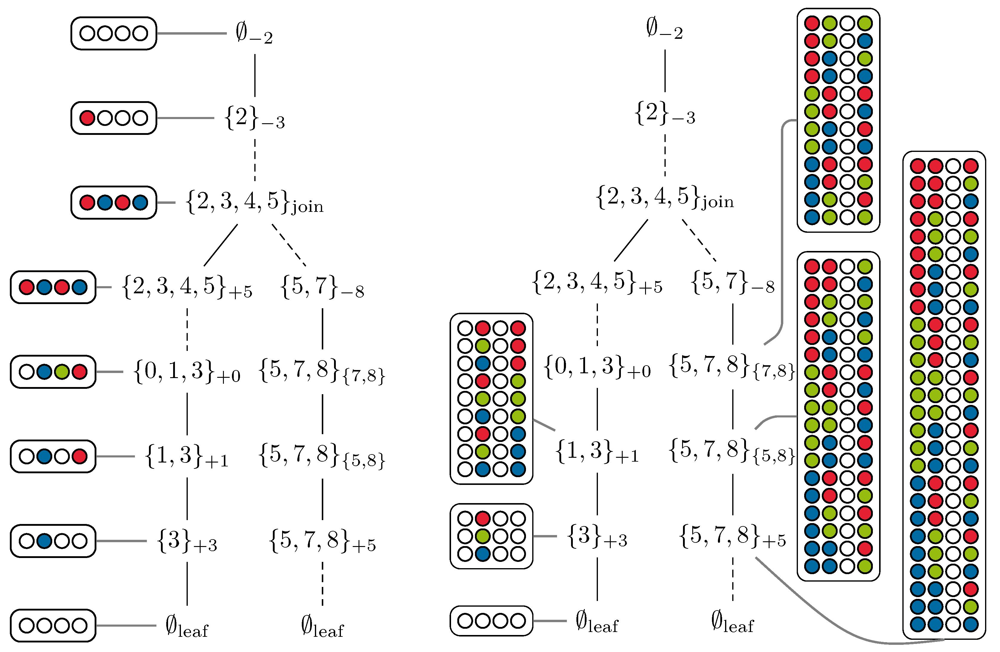
A dynamic program for a decision problem can be formulated as a nondeterministic tree automaton that works on the decomposition—see the left side of Figure 1 for a detailed example. Observe that a nondeterministic tree automaton A will process a labeled tree $(T,\iota )$ with n nodes in time $O(n)$. When we simulate such an automaton deterministically, one might think that a running time of the form $O(|Q|·n)$ is sufficient, as the automaton could be in any potential subset of the Q states at some node of the tree. However, there is a pitfall: for every node, we have to compute the set of potential states of the automaton depending on the sets of potential states of the children of that node, leading to a quadratic dependency on $\left|Q\right|$. This can be avoided for transitions of the form $(\perp ,\perp ,\iota (x),p)$, $(q,\perp ,\iota (x),p)$, and $(\perp ,q,\iota (x),p)$, as we can collect potential successors of every state of the child and compute the new set of states in linear time with respect to the cardinality of the set. However, transitions of the form $(q_i,q_j,\iota (x),p)$ are difficult, as we now have to merge two sets of states. In detail, let x be a node with children y and z and let $Q_y$ and $Q_z$ be the set of potential states in which the automaton eventually is in at these nodes. To determine $Q_x$, we have to check for every $q_i\in Q_y$ and every $q_j\in Q_z$ if there is a $p\in Q$ such that $(q_i,q_j,\iota (x),p)\in \mathsf{\Delta }$. Note that the number of states $\left|Q\right|$ can be quite large, as for tree decompositions with bags of size k the set Q is typically of cardinality $2^{\mathsf{\Omega }(k)}$, and we will thus try to avoid this quadratic blow-up.

Observation 1.

A tree automaton can be simulated in time $O(|Q{|}^2·n)$.

Unfortunately, the quadratic factor in the simulation cannot be avoided in general, as the automaton may very well contain a transition for all possible pairs of states. However, there are some special cases in which we can circumnavigate the increase in the running time.

Definition 3 (Symmetric Tree Automaton).

A symmetric nondeterministic bottom-up tree automaton is a nondeterministic bottom-up tree automaton $A=(Q,\mathsf{\Sigma },\mathsf{\Delta },F)$ in which all transitions $(l,r,\sigma ,q)\in \mathsf{\Delta }$ satisfy either $l=\perp$, $r=\perp$, or $l=r$.

Assume as before that we wish to compute the set of potential states for a node x with children y and z. Observe that, in a symmetric tree automaton, it is sufficient to consider the set $Q_y\cap Q_z$ and that the intersection of two sets can be computed in linear time if we take some care in the design of the underlying data structures.

Observation 2.

A symmetric tree automaton can be simulated in time $O(|Q|·n)$.

The right side of Figure 1 illustrates the deterministic simulation of a symmetric tree automaton. The massive time difference in the simulation of tree automata and symmetric tree automata significantly influenced the design of the algorithms in Section 4, in which we try to construct an automaton that is (1) “as symmetric as possible” and (2) allows for taking advantage of the “symmetric parts” even if the automaton is not completely symmetric.

3.2. The Interface

We introduce a simple Java-interface to our library Jdrasil, which originally was developed for the computation of tree decompositions only. The interface is built up from two classes: StateVectorFactory and StateVector. The only job of the factory is to generate StateVector objects for the leaves of the tree decomposition, or with the terms of the previous section: “to define the initial states of the tree automaton.” The StateVector class is meant to model a vector of potential states in which the nondeterministic tree automaton is at a specific node of the tree decomposition. Our interface does not define what a “state” is, or how a collection of states is managed. The only thing the interface requires a user to implement is the behaviour of the tree automaton when it reaches a node of the tree decomposition, i.e., given a StateVector for some node x of the tree decomposition and the information that the next node y reached by the automaton is of a certain type, the user has to compute the StateVector for y. To this end, the interface contains the methods shown in Listing 1.

Listing 1: The four methods of the interface describe the behaviour of the tree automaton. Here, “T” is a generic type for vertices. Each function obtains as a parameter the current bag and a tree-index “idx”. Other parameters correspond to bag-type specifics, e.g., the introduced or forgotten vertex v.

StateVector<T> introduce(Bag<T> b, T v, Map<T, Integer> idx);
StateVector<T> forget(Bag<T> b, T v, Map<T, Integer> idx);
StateVector<T> join(Bag<T> b, StateVector<T> o, Map<T, Integer> idx);
StateVector<T> edge(Bag<T> b, T v, T w, Map<T, Integer> idx);
		

This already rounds up the description of the interface, everything else is done by Jdrasil. In detail, given a graph and an implementation of the interface, Jdrasil will compute a tree decomposition (see [11] for the concrete algorithms used by Jdrasil), transform this decomposition into a very nice tree decomposition, potentially optimize the tree decomposition for the following dynamic program, and finally traverse through the tree decomposition and simulate the tree automaton described by the implementation of the interface. The result of this procedure is the StateVector object assigned to the root of the tree decomposition.

3.3. Example: 3-Coloring

Let us illustrate the usage of the interface with our running example of 3-coloring. A State of the automaton can be modeled as a simple integer array that stores a color (an integer) for every vertex in the bag. A StateVector stores a set of State objects, that is, essentially a set of integer arrays. Introducing a vertex v to a StateVector therefore means that three duplicates of each stored state have to be created, and, for every duplicate, a different color has to be assigned to v. Listing 2 illustrates how this operation could be realized in Java.

Listing 2: Exemplary implementation of the introduce method for 3-coloring. In the listing, the variable states is stored by the StateVector object and represents all currently possible states.

StateVector<T> introduce(Bag<T> b, T v, Map<T, Integer> idx) {
  Set<State> newStates = new HashSet<>();
  for (State state : states) { // ’states’ is the set of states
   for (int color = 1; color <= 3; color++) {
      State newState = new State(state); // copy the state
      newState.colors[idx.get(v)] = color;
      newStates.add(newState);
    }
  }
  states = newStates;
  return this;
}
		

The three other methods can be implemented in a very similar fashion: in the forget-method, we set the color of v to 0; in the edge-method, we remove states in which both endpoints of the edge have the same color; and, in the join-method, we compute the intersection of the state sets of both StateVector objects. Note that, when we forget a vertex v, multiple states may become identical, which is handled here by the implementation of the Java Set-class, which takes care of duplicates automatically.

A reference implementation of this 3-coloring solver is publicly available [12], and a detailed description of it can be found in the manual of Jdrasil [13]. Note that this implementation is only meant to illustrate the interface and that we did not make any effort to optimize it. Nevertheless, this very simple implementation (the part of the program that is responsible for the dynamic program only contains about 120 lines of structured Java-code) performs surprisingly well.

4. A Lightweight Model Checker for an MSO-Fragment

Experiments with the coloring solver of the previous section have shown a huge difference in the performance of general solvers as D-Flat and Sequoia against a concrete implementation of a tree automaton for a specific problem (see Section 5). This is not necessarily surprising, as a general solver needs to keep track of way more information. In fact, an MSO model checker on formula $\varphi$ can probably (unless $\mathrm{P}=\mathrm{NP}$) not run in time $f(|\varphi |+\mathrm{tw})·\mathrm{poly}(n)$ for any elementary function f [14]. On the other hand, it is not clear (in general) what the concrete running time of such a solver is for a concrete formula or problem (see e.g., [15] for a sophisticated analysis of some running times in Sequoia). We seek to close this gap between (slow) general solvers and (fast) concrete algorithms. Our approach is to concentrate only on a fragment of MSO, which is powerful enough to express many natural problems, but which is restricted enough to allow model checking in time that matches or is close to the running time of a concrete algorithm for the problem. As a bonus, we will be able to derive upper bounds on the running time of the model checker directly from the syntax of the input formula.

Based on the interface of Jdrasil, we have implemented a publicly available prototype called Jatatosk [16]. In Section 5, we describe various experiments on different problems on multiple sets of graphs. It turns out that Jatatosk is competitive against the state-of-the-art solvers D-Flat and Sequoia. Arguably, these two programs solve a more general problem and a direct comparison is not entirely fair. However, the experiments do reveal that it seems very promising to focus on smaller fragments of MSO (or perhaps any other description language) in the design of treewidth based solvers.

4.1. Description of the Used MSO-Fragment

We only consider vocabularies $\tau$ that contain the binary relation $E^2$, and we only consider $\tau$-structures with a symmetric interpretation of $E^2$, that is, we only consider structures that contain an undirected graph (but may also contain further relations). The fragment of MSO that we consider is constituted by formulas of the form $\varphi =\exists X_1\dots \exists X_k{\bigwedge }_{i=1}^n{\psi }_i$, where the $X_j$ are second-order variables and the ${\psi }_i$ are first-order formulas of the form

$$\begin{array}{cc}\hfill {\psi }_i\in \{& \forall x\forall yE(x,y)\to {\chi }_i,\forall x\exists yE(x,y)\wedge {\chi }_i,\exists x\forall yE(x,y)\to {\chi }_i,\hfill \\ & \exists x\exists yE(x,y)\wedge {\chi }_i,\forall x{\chi }_i,\exists x{\chi }_i\}.\hfill \end{array}$$

Here, the ${\chi }_i$ are quantifier-free first-order formulas in canonical normal form. It is easy to see that this fragment is already powerful enough to encode many classical problems as 3-coloring (${\tilde{\varphi }}_{3\mathrm{col}}$ from the introduction is part of the fragment), or vertex-cover (note that, in this form, the formula is not very useful—every graph is a model of the formula if we choose $S=V(G)$; we will discuss how to handle optimization in Section 4.4):

$${\tilde{\varphi }}_{\mathrm{vc}}=\exists S\forall x\forall yE(x,y)\to S(x)\vee S(y).$$

4.2. A Syntactic Extension of the Fragment

Many interesting properties, such as connectivity, can easily be expressed in MSO, but not directly in the fragment that we study. Nevertheless, a lot of these properties can directly be checked by a model checker if it “knows” what kind of properties it actually checks. We present a syntactic extension of our MSO-fragment which captures such properties. The extension consists of three new second order quantifiers that can be used instead of $\exists X_i$.

The first extension is a k-partition quantifier, which quantifies over partitions of the universe:

$${\exists }^{\mathrm{partition}}{X}_1,\dots ,X_k\equiv \exists X_1\exists X_2\dots \exists X_k(\forall x\underset{i=1}{\overset{k}{\bigvee }}{X}_i(x))\wedge (\forall x\underset{i=1}{\overset{k}{\bigwedge }}\underset{j\ne i}{\bigwedge }\neg X_i(x)\wedge \neg X_j(x)).$$

This quantifier has two advantages. First, formulas like ${\tilde{\varphi }}_{3\mathrm{col}}$ can be simplified to

$${\varphi }_{3\mathrm{col}}={\exists }^{\mathrm{partition}}R,G,B\forall x\forall yE(x,y)\to \underset{C\in \{R,G,B\}}{\bigwedge }\neg C(x)\vee \neg C(y),$$

and, second, the model checking problem for them can be solved more efficiently: the solver directly “knows” that a vertex must be added to exactly one of the sets.

We further introduce two quantifiers that work with respect to the symmetric relation $E^2$ (recall that we only consider structures that contain such a relation). The ${\exists }^{\mathrm{connected}}X$ quantifier guesses an $X\subseteq U$ that is connected with respect to E (in graph theoretic terms), that is, it quantifies over connected subgraphs. The ${\exists }^{\mathrm{forest}}F$ quantifier guesses a $F\subseteq U$ that is acyclic with respect to E (again in graph theoretic terms), that is, it quantifies over subgraphs that are forests. These quantifiers are quite powerful and allow, for instance, expressing that the graph induced by $E^2$ contains a triangle as minor:

$$\begin{array}{cc}\hfill {\varphi }_{\mathrm{triangle}-\mathrm{minor}}=& {\exists }^{\mathrm{connected}}R{\exists }^{\mathrm{connected}}G{\exists }^{\mathrm{connected}}B·\hfill \\ & \left(\forall x(\neg R(x)\vee \neg G(x))\wedge (\neg G(x)\vee \neg B(x))\wedge (\neg B(x)\vee \neg R(x))\right)\hfill \\ \hfill \wedge & \left(\exists x\exists yE(x,y)\wedge R(x)\wedge G(y)\right)\wedge \left(\exists x\exists yE(x,y)\wedge G(x)\wedge B(y)\right)\hfill \\ \hfill \wedge & \left(\exists x\exists yE(x,y)\wedge B(x)\wedge R(y)\right).\hfill \end{array}$$

We can also express problems that usually require more involved formulas in a very natural way. For instance, the feedback-vertex-set problem can be described by the following formula (again, optimization will be handled in Section 4.4):

$${\tilde{\varphi }}_{\mathrm{fvs}}=\exists S{\exists }^{\mathrm{forest}}F\forall xS(x)\vee F(x).$$

4.3. Description of the Model Checker

We describe our model checker in terms of a nondeterministic tree automaton that works on a tree decomposition of the graph induced by $E^2$ (note that, in contrast to other approaches in the literature (see, for instance, [10]), we do not work on the Gaifman graph). We define any state of the automaton as a bit-vector, and we stipulate that the initial state at every leaf is the zero-vector. For any quantifier or subformula, there will be some area in the bit-vector reserved for that quantifier or subformula and we describe how state transitions effect these bits. The “algorithmic idea” behind the implementation of these transitions is not new, and a reader familiar with folklore dynamic programs on tree decompositions (for instance for vertex-cover or steiner-tree) will probably recognize them. An overview over common techniques can be found in the standard textbooks [1,10].

4.3.1. The Partition Quantifier

We start with a detailed description of the k-partition quantifier ${\exists }^{\mathrm{partition}}{X}_1,\dots ,X_q$ (in fact, we do not implement an additional $\exists X$ quantifier, as we can always state $\exists X\equiv {\exists }^{\mathrm{partition}}X,\overline{X}$): Let k be the maximum bag-size of the tree decomposition. We reserve $k·{log}_{2}q$ bit in the state description (Here, and in the following, $log(x)$ denotes the number of bits to store x, i.e., $log(x)=\lfloor {log}_2(x)\rfloor +1$), where each block of length $logq$ indicates in which set $X_i$ the corresponding element of the bag is. On an introduce-bag (e.g., for $v\in U$), the nondeterministic automaton guesses an index $i\in \{1,\dots ,q\}$ and sets the $logq$ bits that are associated with the tree-index of v to i. Equivalently, the corresponding bits are cleared when the automaton reaches a forget-bag. As the partition is independent of any edges, an edge-bag does not change any of the bits reserved for the k-partition quantifier. Finally, on join-bags, we may only join states that are identical on the bits describing the partition (as otherwise the vertices of the bag would be in different partitions)—meaning this transition is symmetric with respect to these bits (in terms of Section 3.1).

4.3.2. The Connected Quantifier

The next quantifier we describe is ${\exists }^{\mathrm{connected}}X$, which has to overcome the difficulty that an introduced vertex may not be connected to the rest of the bag in the moment it got introduced, but may be connected to it when further vertices “arrive.” The solution to this dilemma is to manage a partition of the bag into $k^{\prime }\le k$ connected components $P_1,\dots ,P_{k^{\prime }}$, for which we reserve $k·logk$ bit in the state description. Whenever a vertex v is introduced, the automaton either guesses that it is not contained in X and clears the corresponding bits, or it guesses that $v\in X$ and assigns some $P_i$ to v. Since v is isolated in the bag in the moment of its introduction (recall that we work on a very nice tree decomposition), it requires its own component and is therefore assigned to the smallest empty partition $P_i$. When a vertex v is forgotten, there are four possible scenarios:

• $v\notin X$, then the corresponding bits are already cleared and nothing happens;
• $v\in X$ and $v\in P_i$ with $|P_i|>1$, then v is just removed and the corresponding bits are cleared;
• $v\in X$ and $v\in P_i$ with $|P_i|=1$ and there are other vertices w in the bag with $w\in X$, then the automaton rejects the configuration, as v is the last vertex of $P_i$ and may not be connected to any other partition anymore;
• $v\in X$ is the last vertex of the bag that is contained in X, then the connected component is “done”, the corresponding bits are cleared and one additional bit is set to indicate that the connected component cannot be extended anymore.

When an edge $\{u,v\}$ is introduced, components might need to be merged. Assume $u,v\in X$, $u\in P_i$, and $v\in P_j$ with $i<j$ (otherwise, an edge-bag does not change the state), then we essentially perform a classical union-operation from the well-known union-find data structure. Hence, we assign all vertices that are assigned to $P_j$ to $P_i$. Finally, at a join-bag, we may join two states that agree locally on the vertices that are in X (that is, they have assigned the same vertices to some $P_i$); however, they do not have to agree in the way the different vertices are assigned to $P_i$ (in fact, there does not have to be an isomorphism between these assignments). Therefore, the transition at a join-bag has to connect the corresponding components analogous to the edge-bags—in terms of Section 3.1, this transition is not symmetric.

The description of the remaining quantifiers and subformulas is very similar and summarized in the following overview:

4.4. Extending the Model Checker to Optimization Problems

As the example formulas from the previous section already indicate, performing model checking alone will not suffice to express many natural problems. In fact, every graph is a model of the formula ${\tilde{\varphi }}_{\mathrm{vc}}$ if S simply contains all vertices. It is therefore a natural extension to consider an optimization version of the model checking problem, which is usually formulated as follows [1,10]: Given a logical structure $\mathcal{S}$, a formula $\varphi (X_1,\dots ,X_p)$ of the MSO-fragment defined in the previous section with free unary second-order variables $X_1,\dots ,X_p$, and weight functions ${\omega }_1,\dots ,{\omega }_p$ with ${\omega }_i:U\to \mathbb{Z}$; find $S_1,\dots ,S_p$ with $S_i\subseteq U$ such that ${\sum }_{i=1}^p{\sum }_{s\in S_i}{\omega }_i(s)$ is minimized under $\mathcal{S}\models \varphi (S_1,\dots ,S_p)$, or conclude that $\mathcal{S}$ is not a model for $\varphi$ for any assignment of the free variables. We can now correctly express the (actually weighted) optimization version of vertex-cover as follows:

$${\varphi }_{\mathrm{vc}}(S)=\forall x\forall yE(x,y)\to \left(S(x)\vee S(y)\right).$$

Similarly, we can describe the optimization version of dominating-set if we assume the input does not have isolated vertices (or is reflexive), and we can also fix the formula ${\tilde{\varphi }}_{\mathrm{fvs}}$:

$$\begin{array}{cc}\hfill {\varphi }_{\mathrm{ds}}(S)& =\forall x\exists yE(x,y)\wedge \left(S(x)\vee S(y)\right),\hfill \\ \hfill {\varphi }_{\mathrm{fvs}}(S)& ={\exists }^{\mathrm{forest}}F\forall x\left(S(x)\vee F(x)\right).\hfill \end{array}$$

We can also maximize the term ${\sum }_{i=1}^p{\sum }_{s\in S_i}{\omega }_i(s)$ by multiplying all weights with $-1$ and, thus, express problems such as independent-set:

$${\varphi }_{\mathrm{is}}(S)=\forall x\forall yE(x,y)\to \left(\neg S(x)\vee \neg S(y)\right).$$

The implementation of such an optimization is straightforward: there is a 2-partition quantifier for every free variable $X_i$ that partitions the universe into $X_i$ and ${\overline{X}}_i$. We assign a current value of ${\sum }_{i=1}^p{\sum }_{s\in S_i}{\omega }_i(s)$ to every state of the automaton, which is adapted if elements are “added” to some of the free variables at introduce nodes. Note that, since we optimize an affine function, this does not increase the state space: even if multiple computational paths lead to the same state with different values at some node of the tree, it is well defined which of these values is the optimal one. Therefore, the cost of optimization only lies in the partition quantifier, that is, we pay with k bits in the state description of the automaton per free variable—independently of the weights (Of course, for each state, we still have to store the weight and we have to perform arithmetic operations on these weights).

4.5. Handling Symmetric and Non-Symmetric Joins

In Section 4.3, we have defined the states of our automaton with respect to a formula,

Table 1. The table shows the precise number of bits we reserve in the description of a state of the tree automaton for different quantifiers and formulas. The values are with respect to a tree decomposition with maximum bag size k.

Quantifier/Formula	Number of Bits
free variables $X_1,\dots ,X_q$	$q·k$
${\exists }^{\mathrm{partition}}{X}_1,\dots ,X_q$	$k·logq$
${\exists }^{\mathrm{connected}}X$	$k·logk+1$
${\exists }^{\mathrm{forest}}X$	$k·logk$
$\forall x\forall yE(x,y)\to {\chi }_i$	0
$\forall x\exists yE(x,y)\wedge {\chi }_i$	k
$\exists x\forall yE(x,y)\to {\chi }_i$	$k+1$
$\exists x\exists yE(x,y)\wedge {\chi }_i$	1
$\forall x{\chi }_i$	0
$\exists x{\chi }_i$	1

gives an overview of the number of bits we require for the different parts of the formula. Let $\mathrm{bit}(\varphi ,k)$ be the number of bits that we have to reserve for a formula $\varphi$ and a tree decomposition of maximum bag size k that is, the sum over the required bits of each part of the formula. By Observation 1, this implies that we can simulate the automaton (and hence solve the model checking problem) in time $O^{*}({(2^{\mathrm{bit}(\varphi ,k)})}^2)$, or by Observation 2 in time $O^{*}(2^{\mathrm{bit}(\varphi ,k)}),$ if the automaton is symmetric (The notation $O^{*}$ supresses polynomial factors). Unfortunately, this is not always the case, in fact, only the quantifier ${\exists }^{\mathrm{partition}}{X}_1,\dots ,X_q$, the bits needed to optimize over free variables, as well as the formulas that do not require any bits, yield a symmetric tree automaton. This means that the simulation is wasteful if we consider a mixed formula (for instance, one that contains a partition and a connected quantifier). To overcome this issue, we partition the bits of the state description into two parts: first, the “symmetric” bits of the quantifiers ${\exists }^{\mathrm{partition}}{X}_1,\dots ,X_q$ and the bits required for optimization, and in the “asymmetric” ones of all other elements of the formula. Let $\mathrm{symmetric}(\varphi ,k)$ and $\mathrm{asymmetric}(\varphi ,k)$ be defined analogously to $\mathrm{bit}(\varphi ,k)$. We implement the join of states as in the following lemma, allowing us to deduce the running time of the model checker for concrete formulas.

Table 2. The table gives an overview of formulas $\varphi$ used within this paper, together with the values $\mathrm{symmetric}(\varphi ,k)$ and $\mathrm{asymmetric}(\varphi ,k)$, as well as the precise time our algorithm will require to model check an instance for that particular formula.

$\mathit{\varphi }$	$\mathbf{symmetric}(\mathit{\varphi },\mathit{k})$	$\mathbf{asymmetric}(\mathit{\varphi },\mathit{k})$	Time
${\varphi }_{3\mathrm{col}}$	$k·log(3)$	0	$O^{*}(3^k)$
${\varphi }_{\mathrm{vc}}(S)$	k	0	$O^{*}(2^k)$
${\varphi }_{\mathrm{ds}}(S)$	k	k	$O^{*}(8^k)$
${\varphi }_{\mathrm{triangle}-\mathrm{minor}}$	0	$3k·log(k)+3$	$O^{*}(k^{6k})$
${\varphi }_{\mathrm{fvs}}(S)$	k	$k·log(k)$	$O^{*}(2^k{k}^{2k})$

provides an overview for formulas presented here.

Lemma 1.

Let x be a join node of T with children y and z, and let $Q_y$ and $Q_z$ be sets of states in which the automaton may be at y and z. Then, the set $Q_x$ of states in which the automaton may be at node x can be computed in time $O^{*}(2^{\mathrm{symmetric}(\varphi ,k)+2·\mathrm{asymmetric}(\varphi ,k)})$.

Proof. 

To compute $Q_x$, we first split $Q_y$ into $B_1,\dots ,B_q$ such that all elements in one $B_i$ share the same “symmetric bits.” This can be done in time $|Q_y|$ using bucket-sort. Note that we have $q\le 2^{\mathrm{symmetric}(\varphi ,k)}$ and $|B_i|\le 2^{\mathrm{asymmetric}(\varphi ,k)}$. With the same technique, we identify for every element v in $Q_z$ its corresponding partition $B_i$. Finally, we compare v with the elements in $B_i$ to identify those for which there is a transition in the automaton. This yields an overall running time of the form $|Q_z|·{max}_{i=1}^q\left|B_i\right|\le 2^{\mathrm{bit}(\varphi ,k)}·2^{\mathrm{asymmetric}(\varphi ,k)}=2^{\mathrm{symmetric}(\varphi ,k)+2·\mathrm{asymmetric}(\varphi ,k)}$. □

5. Applications and Experiments

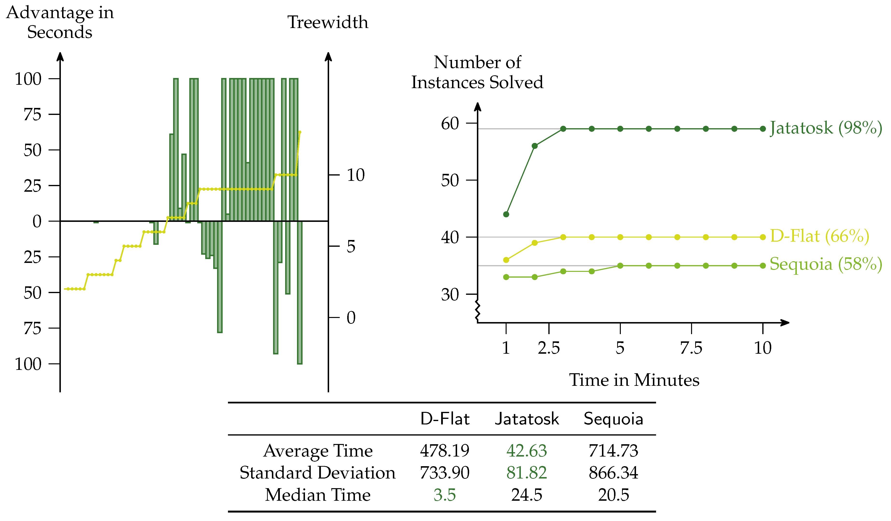
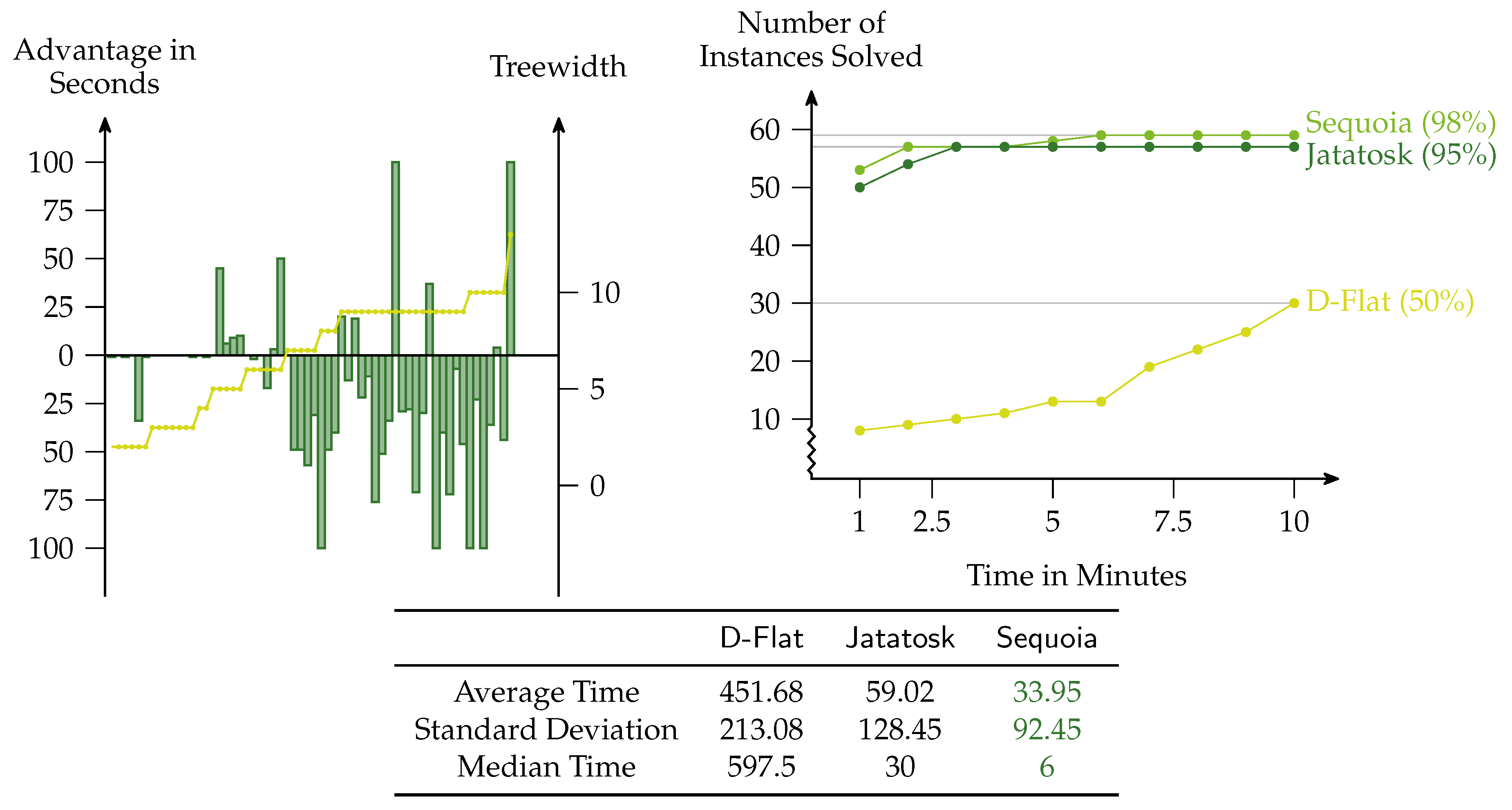
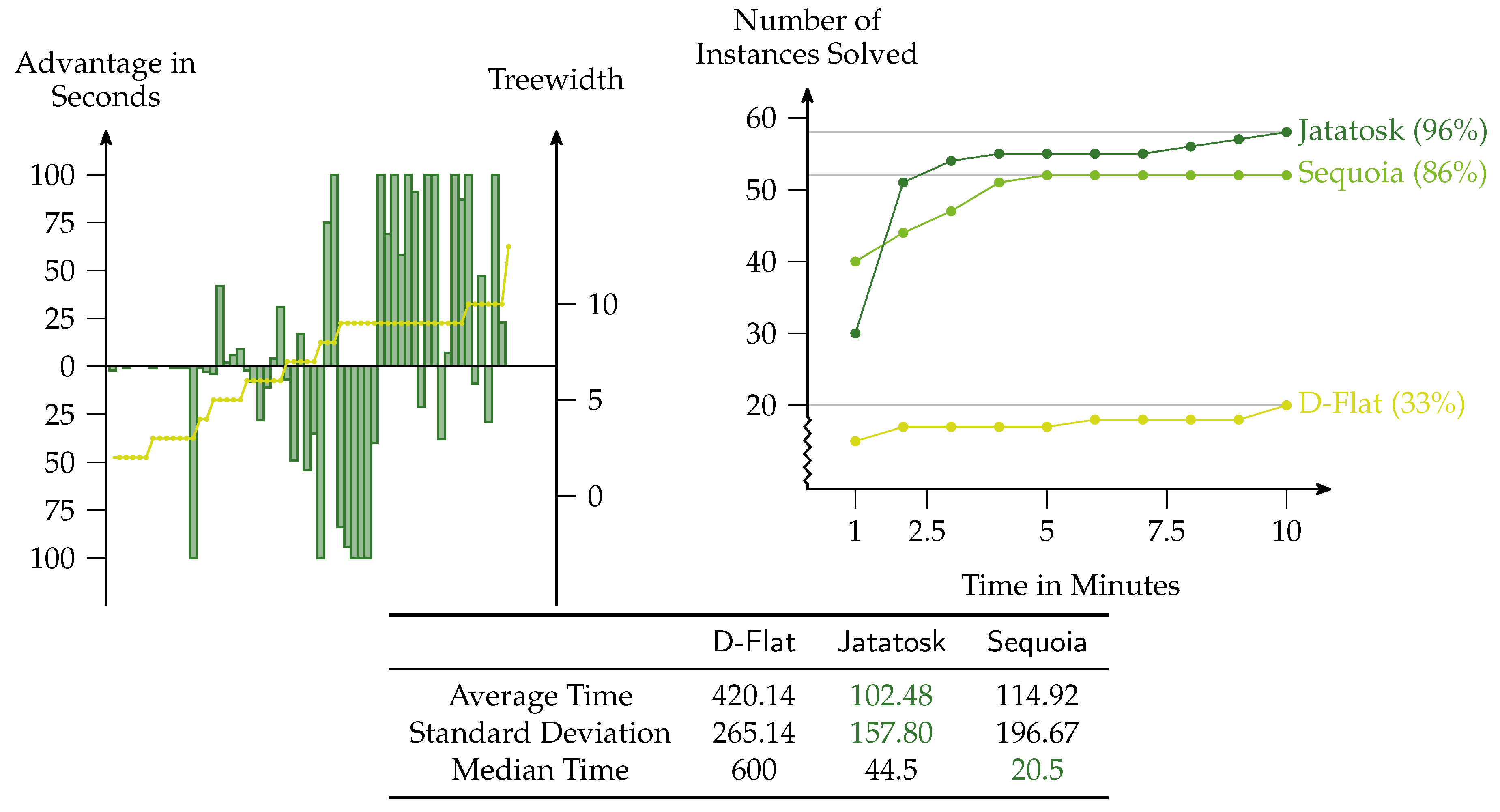
To show the feasibility of our approach, we have performed experiments for widely investigated graph problems: 3-coloring (Figure 2), vertex-cover (Figure 3), dominating-set (Figure 4), independent-set (Figure 5), and feedback-vertex-set (Figure 6). All experiments were performed on an Intel Core processor containing four cores of 3.2 GHz each and 8 Gigabyte RAM. Jdrasil was used with Java 8.1 and both Sequoia and D-Flat were compiled with gcc 7.2. All compilations were performed with the default optimization settings. The implementation of Jatatosk uses hashing to realize Lemma 1, which works well in practice. We use a data set assembled from different sources containing graphs with 18 to 956 vertices and treewidth 3 to 13. 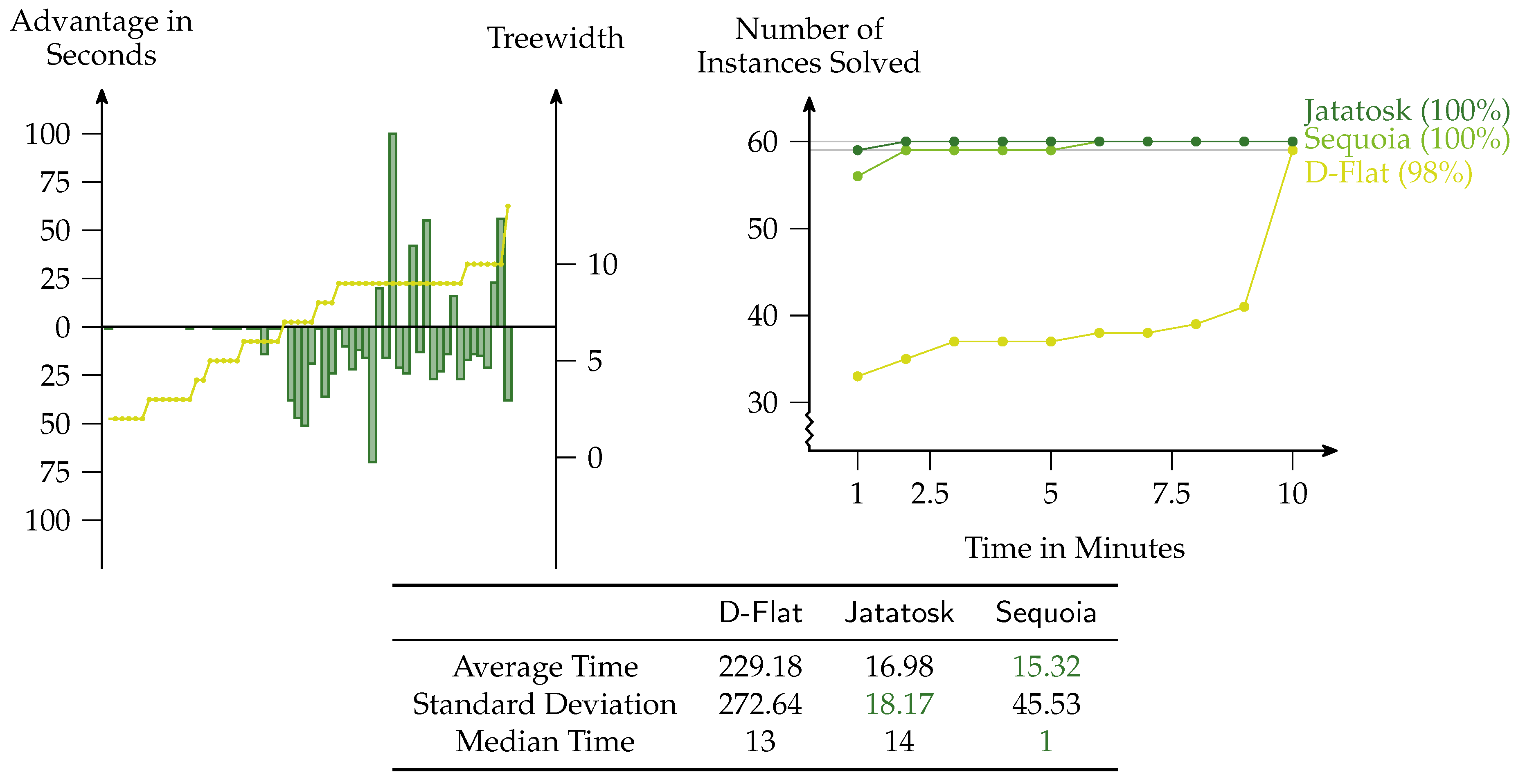The first source is a collection of transit graphs from GTFS-transit feeds [17] that was also used for experiments in [18], the second source is real-world instances collected in [19], and the last one is that of the PACE challenge [2] with treewidth at most 11. In each of the experiments, the left picture always shows the difference of Jatatosk against D-Flat and Sequoia. A positive bar means that Jatatosk is faster by this amount in seconds, and a negative bar means that either D-Flat or Sequoia is faster by that amount. The bars are capped at 100 seconds. 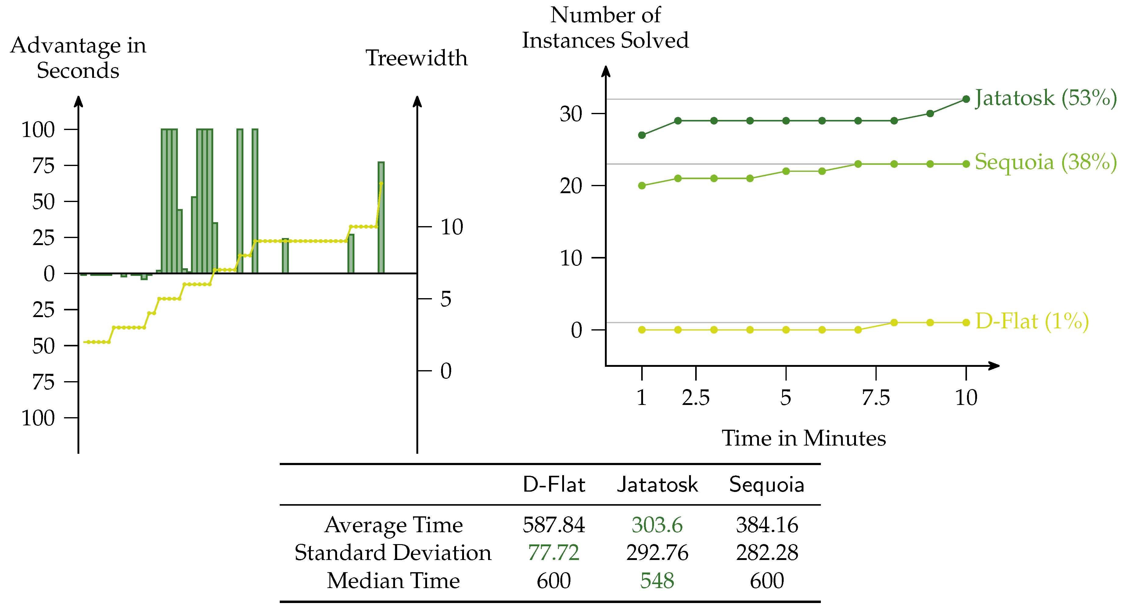On every instance, Jatatosk was compared against the solver that was faster on this particular instance. The image also shows for every instance the treewidth of the input. The right image always shows a cactus plot that visualizes the number of instances that can be solved by each of the solvers in x seconds, that is, faster growing functions are better. For each experiment, there is a table showing the average, standard deviation, and median of the time (in seconds) each solver needed to solve the problem. The best values are highlighted.

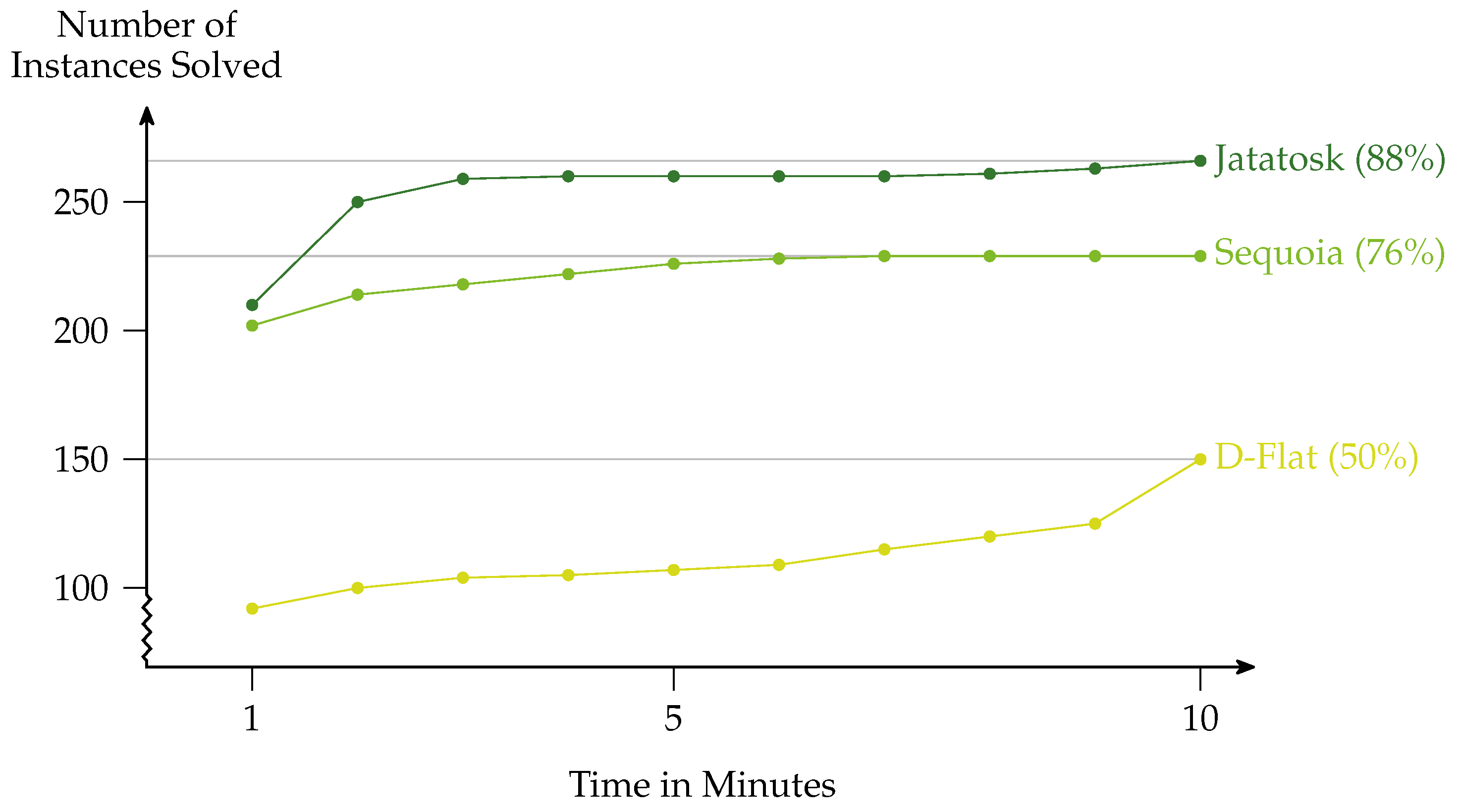
The experiments reveal that Jatatosk is faster than its competitors on many instances. However, there are also formulas such as the one for the vertex cover problem on which one of the other solvers performs better on some of the instances. For an overall picture, the cactus plot in Figure 7 is the sum of all cactus plots from the experiments. It reveals that overall Jatatosk in fact outperforms its competitors. However, we stress once more that the comparison is not completely fair, as both Sequoia and D-Flat are powerful enough to model check the whole of MSO (and actually also ${\mathrm{MSO}}_2$), while Jatatosk can only handle a fragment of ${\mathrm{MSO}}_1$.

As we can see, Jatatosk outperforms Sequoia and D-Flat if we consider the graph coloring problem. Its average time is more than a factor of 10 smaller than the average time of its competitors and Jatatosk solves about 30% of the instances more. This result is not surprising, as the fragment used by Jatatosk is directly tailored towards coloring and, thus, Jatatosk has a natural advantage.

The vertex-cover problem is solved best by Sequoia, which becomes apparent if we consider the difference plot. Furthermore, the average time used by Sequoia is better than the time used by Jatatosk. However, considering the cactus plot, the difference between Jatatosk and Sequoia with respect to solved instances is small, while D-Flat falls behind a bit. We assume that the similarity between Jatatosk and Sequoia is because both compile internally a similar algorithm.

In this experiment Jatatosk performs best with respect to all: the difference plot, the cactus plot, and the used average time. However, the difference to Sequoia is small and there are in fact a couple of instances that are solved faster by Sequoia. We are surprised by this result, as the worst-case running time of Jatatosk for dominating-set is $O^{*}(8^k)$ and, thus, far from optimal. Furthermore, Sequoia promises in theory a better performance with a running time of the form $O^{*}(5^k)$ [15].

This is the simplest test set that we consider within this paper, which is reflected by the fact that all solvers are able to solve almost the whole set. The difference between Jatatosk and Sequoia is minor: while Jatatosk has a slightly better peek-performance, there are more instances that are solved faster by Sequoia than the other way around.

This is the hardest test set that we consider within this paper, which is reflected by the fact that no solver is able to solve much more than 50% of the instances. Jatatosk outperforms its competitors, which is reflected in the difference plot, the cactus plot, and the used average time. We assume this is because Jatatosk uses the dedicated forest quantifier directly, while the other tools have to infer the algorithmic strategy from a more general formula.

6. Conclusions and Outlook

We investigated the practicability of dynamic programming on tree decompositions, which is arguably one of the cornerstones of parameterized complexity theory. We implemented a simple interface for such programs and used it to build a competitive graph coloring solver with just a few lines of code. We hope that this interface allows others to implement and explore various dynamic programs. The whole power of these algorithms is well captured by Courcelle’s Theorem, which states that there is an efficient version of such a program for every problem definable in monadic second-order logic. We took a step towards practice by implementing a “lightweight” version of a model checker for a small fragment of the logic. This fragment turns out to be powerful enough to express many natural problems such as 3-coloring, feedback-vertex-set, and more. Various experiments showed that the model checker is competitive against the state-of-the-art solvers D-Flat and Sequoia. It therefore seems promising, from a practical perspective, to study smaller fragments of MSO.