A Compendium of Parameterized Problems at Higher Levels of the Polynomial Hierarchy

Abstract

We present a list of parameterized problems together with a complexity classification of whether they allow a fixed-parameter tractable reduction to SAT or not. These problems are parameterized versions of problems whose complexity lies at the second level of the Polynomial Hierarchy or higher.

1. Introduction

The remarkable performance of today’s SAT solvers (see, e.g., [1]) offers a practically successful strategy for solving NP-complete combinatorial search problems by reducing them in polynomial time to the propositional satisfiability problem—also known as SAT. In order to apply this strategy to problems that are harder than NP, one needs to employ reductions that are more powerful than polynomial-time reductions. A compelling option for this strategy is to use fixed-parameter tractable reductions (or fpt-reductions)—i.e., reductions that are computable in time $f\left(k\right)n^c$ for some computable function f and some constant c—as they can exploit some structural aspects of the problem instances in terms of a problem parameter k.

To illustrate this approach, let us consider as an example the problem of deciding the truth of quantified Boolean formulas (QBFs) of the form $\phi =\exists X.\forall Y.\psi$, where $\psi$ is a DNF formula over the variables in $X\cup Y$. (We define and consider this example problem—as well as the parameterized variants of this problem that we consider in this section—in more detail in Section 3.3.) This problem is ${\Sigma }_2^{\mathrm{p}}$-complete [2,3], so there is no polynomial-time reduction from this problem to SAT, unless the Polynomial Hierarchy collapses. In other words, the strategy of first reducing the problem to SAT, and then using a SAT solver to solve the problem seems not viable.

Another strategy would be to consider the problem from a parameterized point of view—i.e., investigating in which cases structural properties of the input allow the problem to be solved efficiently (in fpt-time). For example, if the incidence treewidth of the DNF formula $\psi$ is bounded, we can solve the problem in fpt-time [4,5]. However, this is the case only in very restricted settings, and so this strategy is also only viable to a limited extent.

The approach of using fpt-reductions to SAT combines the merits of the above two strategies. It uses the remarkable performance of today’s SAT solvers, and it can exploit structural properties of the problem inputs. As a result, this approach has the potential of being useful in a much wider range of settings than either of the two separate strategies. It can work for problems that lie at higher levels of the Polynomial Hierarchy. Moreover, it can work for choices of problem parameters that are much less restrictive than those needed to get traditional fixed-parameter tractability results.

As a demonstration of this, let us consider two other parameterized variants of our example problem of deciding the truth of formulas of the form $\phi =\exists X.\forall Y.\psi$. In the first variant, the parameter is the treewidth of the incidence graph of $\psi$ where we delete all nodes corresponding to variables in X—in other words, the incidence graph of $\psi$ with respect to the universally quantified variables. This variant is para-NP-complete [6,7], which means that it allows an fpt-reduction to SAT. Thus, for this variant, we can exploit the problem parameter to efficiently reduce the problem to SAT, and subsequently use a SAT solver to solve the problem. In the second variant that we consider, the parameter is the treewidth of the incidence graph of $\psi$ where we delete all nodes corresponding to variables in Y—in other words, the incidence graph of $\psi$ with respect to the existentially quantified variables. This variant is para-${\Sigma }_2^{\mathrm{p}}$-complete [6,7], indicating that fpt-reductions to SAT are not possible (unless the Polynomial Hierarchy collapses).

For both of these variants of our example problem, both the approach of polynomial-time reducing the problem to SAT and the approach of finding (traditional) fixed-parameter tractable algorithms do not work. However, for only one of them, an fpt-reduction to SAT is possible (under common complexity-theoretic assumptions). This indicates that, to establish whether an fpt-reduction to SAT is possible, a suitable parameterized complexity analysis at higher levels of the Polynomial Hierarchy is needed. Various parameterized complexity classes have been developed for this purpose [7,8] that, together with previously studied classes, enable such analyses. This includes both classes that correspond to various types of fpt-reductions to SAT—e.g., para-NP, para-co-NP, and ${\mathrm{FPT}}^{\mathrm{NP}}\left[\mathrm{few}\right]$—and classes that indicate that no fpt-reductions to SAT are possible, under suitable complexity-theoretic assumptions—e.g., ${\Sigma }_2^{\mathrm{p}}[k\ast ]$, ${\Sigma }_2^{\mathrm{p}}[\ast k,1]$, ${\Sigma }_2^{\mathrm{p}}[\ast k,\mathrm{P}]$, ${\Pi }_2^{\mathrm{p}}[k\ast ]$, ${\Pi }_2^{\mathrm{p}}[\ast k,1]$, ${\Pi }_2^{\mathrm{p}}[\ast k,\mathrm{P}]$, para-${\Sigma }_2^{\mathrm{p}}$, para-${\Pi }_2^{\mathrm{p}}$, PH$\left[\mathrm{level}\right]$, and para-PSPACE. (We define all of these parameterized complexity classes in Section 2.2 and Section 2.3.)

Outline

In this compendium, we give a list of parameterized problems that are based on problems at higher levels of the Polynomial Hierarchy, together with a complexity classification indicating whether they allow a (many-to-one or Turing) fpt-reduction to SAT or not.

The compendium that we provide is similar in concept to the compendia by Schaefer and Umans [9] and Cesati [10] that also list problems along with their computational complexity. We group the list by the type of problems. A list of problems grouped by their complexity can be found at the end of this paper.

The remainder of the paper is structured as follows. In Section 2, we give an overview of the parameterized complexity classes involved in the classification of whether problems allow an fpt-reduction to SAT, as well as some other notions and definitions that are used throughout the paper. Then, in Section 3, Section 4, Section 5 and Section 6, we present (i) problems related to (quantified variants of) propositional logic, (ii) problems from the area of Knowledge Representation and Reasoning, (iii) graph problems, and (iv) other problems, respectively. Finally, we conclude in Section 7.

2. Preliminaries

2.1. Computational Complexity

We assume that the reader is familiar with basic notions from the theory of computational complexity, such as the complexity classes P and NP. For more details, we refer to textbooks on the topic (see, e.g., [11,12]).

There are many natural decision problems that are not contained in the classical complexity classes P and NP (under some common complexity-theoretic assumptions). The Polynomial Hierarchy [2,3,12,13] contains a hierarchy of increasing complexity classes ${\Sigma }_i^{\mathrm{p}}$, for all $i\ge 0$. We give a characterization of these classes based on the satisfiability problem of various classes of quantified Boolean formulas. A quantified Boolean formula is a formula of the form $Q_1{X}_1{Q}_2{X}_2\cdots Q_m{X}_m\psi$, where each $Q_i$ is either ∀ or ∃, the $X_i$ are disjoint sets of propositional variables, and $\psi$ is a Boolean formula over the variables in ${\bigcup }_{i=1}^m{X}_i$. The quantifier-free part of such formulas is called the matrix of the formula. Truth of such formulas is defined in the usual way. Let $\gamma =\{x_1\mapsto d_1,\cdots ,x_n\mapsto d_n\}$ be a function that maps some variables of a formula $\phi$ to other variables or to truth values. We let $\phi \left[\gamma \right]$ denote the application of such a substitution $\gamma$ to the formula $\phi$. We also write $\phi [x_1\mapsto d_1,\cdots ,x_n\mapsto d_n]$ to denote $\phi \left[\gamma \right]$. For each $i\ge 1$, the decision problem QSat${}_i$ is defined as follows.

QSat${}_i$ Instance: A quantified Boolean formula $\phi =\exists X_1\forall X_2\exists X_3\cdots Q_i{X}_i\psi$, where $Q_i$ is a universal quantifier if i is even and an existential quantifier if i is odd. Question: Is $\phi$ true?

Input formulas to the problem QSat${}_i$ are called ${\Sigma }_i^{\mathrm{p}}$-formulas. For each nonnegative integer $i\ge 0$, the complexity class ${\Sigma }_i^{\mathrm{p}}$ can be characterized as the closure of the problem QSat${}_i$ under polynomial-time reductions [2,3]—that is, all decision problems that are polynomial-time reducible to QSat${}_i$. The ${\Sigma }_i^{\mathrm{p}}$-hardness of QSat${}_i$ holds already when the matrix of the input formula is restricted to $3\mathrm{CNF}$ for odd i, and restricted to $3\mathrm{DNF}$ for even i. Note that the class ${\Sigma }_0^{\mathrm{p}}$ coincides with P, and the class ${\Sigma }_1^{\mathrm{p}}$ coincides with NP. For each $i\ge 1$, the class ${\Pi }_i^{\mathrm{p}}$ is defined as co-${\Sigma }_i^{\mathrm{p}}$—that is, ${\Pi }_i^{\mathrm{p}}=\{{\{0,1\}}^{\ast }\backslash L:L\in {\Sigma }_i^{\mathrm{p}}\}$.

The classes ${\Sigma }_i^{\mathrm{p}}$ and ${\Pi }_i^{\mathrm{p}}$ can also be defined by means of nondeterministic Turing machines with an oracle. Intuitively, oracles are black-box machines that can solve a problem in a single time step—for more details, see, e.g., Chapter 3 of [11]. For any complexity class C, we let ${\mathrm{NP}}^C$ be the set of decision problems that are decided in polynomial time by a nondeterministic Turing machine with an oracle for a problem that is in the class C. Then, the classes ${\Sigma }_i^{\mathrm{p}}$ and ${\Pi }_i^{\mathrm{p}}$, for $i\ge 0$, can be equivalently defined by letting ${\Sigma }_0^{\mathrm{p}}={\Pi }_0^{\mathrm{p}}=\mathrm{P}$, and for each $i\ge 1$ letting ${\Sigma }_i^{\mathrm{p}}={\mathrm{NP}}^{{\Sigma }_{i-1}^{\mathrm{p}}}$ and ${\Pi }_i^{\mathrm{p}}={\mathrm{co-NP}}^{{\Sigma }_{i-1}^{\mathrm{p}}}$.

The Polynomial Hierarchy also includes complexity classes between ${\Sigma }_i^{\mathrm{p}}$ and ${\Sigma }_{i+1}^{\mathrm{p}}$—such as the classes ${\Delta }_{i+1}^{\mathrm{p}}$ and ${\Theta }_{i+1}^{\mathrm{p}}$. The class ${\Delta }_{i+1}^{\mathrm{p}}$ consists of all decision problems that are decided in polynomial time by a deterministic Turing machine with an oracle for a problem that is in the class ${\Sigma }_i^{\mathrm{p}}$. Similarly, the class ${\Theta }_{i+1}^{\mathrm{p}}$ consists of all decision problems that are decided in polynomial time by a deterministic Turing machine with an oracle for a problem that is in the class ${\Sigma }_i^{\mathrm{p}}$, with the restriction that the Turing machine is only allowed to make $O(logn)$ oracle queries, where n denotes the input size [14,15]. It holds that ${\Sigma }_i^{\mathrm{p}}\cup {\Pi }_i^{\mathrm{p}}\subseteq {\Theta }_{i+1}^{\mathrm{p}}\subseteq {\Delta }_{i+1}^{\mathrm{p}}\subseteq {\Sigma }_{i+1}^{\mathrm{p}}\cap {\Pi }_{i+1}^{\mathrm{p}}$.

There are also natural decision problems that are located between NP and ${\Theta }_2^{\mathrm{p}}$. The Boolean Hierarchy (BH) [16,17,18] consists of a hierarchy of complexity classes ${\mathrm{BH}}_i$, for each $i\ge 1$, that can be used to classify the complexity of decision problems between NP and ${\Theta }_2^{\mathrm{p}}$. Each class ${\mathrm{BH}}_i$ can be characterized as the class of problems that can be reduced to the problem ${\mathrm{BH}}_i$-Sat, which is defined inductively as follows. The problem ${\mathrm{BH}}_1$-Sat consists of all sequences $\left(\phi \right)$ of length 1, where $\phi$ is a satisfiable propositional formula. For even $i\ge 2$, the problem ${\mathrm{BH}}_i$-Sat consists of all sequences $({\phi }_1,\cdots ,{\phi }_i)$ of propositional formulas such that both $({\phi }_1,\cdots ,{\phi }_{i-1})\in$${\mathrm{BH}}_{(i-1)}$-Sat and ${\phi }_i$ is unsatisfiable. For odd $i\ge 2$, the problem ${\mathrm{BH}}_i$-Sat consists of all sequences $({\phi }_1,\cdots ,{\phi }_i)$ of propositional formulas such that $({\phi }_1,\cdots ,{\phi }_{i-1})\in$${\mathrm{BH}}_{(i-1)}$-Sat or ${\phi }_i$ is satisfiable. The class ${\mathrm{BH}}_2$ is also denoted by DP, and the problem ${\mathrm{BH}}_2$-Sat is also denoted by $\mathrm{SAT-UNSAT}$. The class BH is defined as the union of all ${\mathrm{BH}}_i$, for $i\ge 1$. It holds that $\mathrm{NP}\cup \mathrm{co-NP}\subseteq {\mathrm{BH}}_2\subseteq {\mathrm{BH}}_3\subseteq \cdots \subseteq \mathrm{BH}\subseteq {\Theta }_2^{\mathrm{p}}$.

2.2. Parameterized Complexity

We introduce some core notions from parameterized complexity theory. For an in-depth treatment, we refer to other sources [19,20,21,22,23]. A parameterized problem L is a subset of ${\Sigma }^{\ast }\times \mathbb{N}$ for some finite alphabet $\Sigma$. For an instance $(x,k)\in {\Sigma }^{\ast }\times \mathbb{N}$, we call x the main part and k the parameter. The following generalization of polynomial-time computability is commonly regarded as the main tractability notion of parameterized complexity theory. A parameterized problem L is fixed-parameter tractable if there exists a computable function f and a constant c such that there exists an algorithm that decides whether $(x,k)\in L$ in time $f\left(k\right)·{\left|x\right|}^c$, where $\left|x\right|$ denotes the size of x. Such an algorithm is called an fpt-algorithm, and this amount of time is called fpt-time. FPT is the class of all parameterized problems that are fixed-parameter tractable. If the parameter is constant, then fpt-algorithms run in polynomial time where the order of the polynomial is independent of the parameter. This provides a good scalability in the parameter in contrast to running times of the form ${\left|x\right|}^k$, which are also polynomial for fixed k, but are already impractical for, say, $k>5$.

Parameterized complexity also generalizes the notion of polynomial-time reductions. Let $L\subseteq {\Sigma }^{\ast }\times \mathbb{N}$ and $L^{\prime }\subseteq {\left({\Sigma }^{\prime }\right)}^{\ast }\times \mathbb{N}$ be two parameterized problems. A (many-one) fpt-reduction from L to $L^{\prime }$ is a mapping $R:{\Sigma }^{\ast }\times \mathbb{N}\to {\left({\Sigma }^{\prime }\right)}^{\ast }\times \mathbb{N}$ from instances of L to instances of $L^{\prime }$ for which there exist some computable function $g:\mathbb{N}\to \mathbb{N}$ such that for all $(x,k)\in {\Sigma }^{\ast }\times \mathbb{N}$: (i) $(x,k)$ is a yes-instance of L if and only if $(x^{\prime },k^{\prime })=R(x,k)$ is a yes-instance of $L^{\prime }$, (ii) $k^{\prime }\le g\left(k\right)$, and (iii) R is computable in fpt-time. Let K be a parameterized complexity class. A parameterized problem L is K-hard if for every $L^{\prime }\in \mathrm{K}$ there is an fpt-reduction from $L^{\prime }$ to L. A problem L is K-complete if it is both in K and K-hard. Reductions that satisfy properties (i) and (ii) but that are computable in time $O\left(\right|x{|}^{f\left(k\right)})$, for some fixed computable function f, we call xp-reductions.

The parameterized complexity classes $\mathrm{W}\left[\mathrm{t}\right]$, for $t\ge 1$, $\mathrm{W}\left[\mathrm{SAT}\right]$, and $\mathrm{W}\left[\mathrm{P}\right]$ can be used to give evidence that a given parameterized problem is not fixed-parameter tractable. These classes are based on the satisfiability problems of Boolean circuits and formulas. We consider Boolean circuits with a single output gate. We call input nodes variables. We distinguish between small gates, with fan-in $\le 2$, and large gates, with fan-in $>2$. The depth of a circuit is the length of a longest path from any variable to the output gate. The weft of a circuit is the largest number of large gates on any path from a variable to the output gate. We say that a circuit C is in negation normal form if all negation nodes in C have variables as inputs. A Boolean formula can be considered as a Boolean circuit where all gates have fan-out $\le 1$. We adopt the usual notions of truth assignments and satisfiability of a Boolean circuit. We say that a truth assignment for a Boolean circuit has weight k if it sets exactly k of the variables of the circuit to true. We denote the class of Boolean circuits with depth u and weft t by ${\mathrm{CIRC}}_{t,u}$. We denote the class of all Boolean circuits by CIRC, and the class of all Boolean formulas by FORM. For any class $\mathcal{C}$ of Boolean circuits, we define the following parameterized problem:

p-WSat$\left[\mathcal{C}\right]$ Instance: A Boolean circuit $C\in \mathcal{C}$, and an integer k. Parameter: k. Question: Does there exist an assignment of weight k that satisfies C?

We denote closure under fpt-reductions by ${[·]}^{\mathrm{fpt}}$—that is, for any set $\mathcal{L}$ of parameterized problems, ${\left[\mathcal{L}\right]}^{\mathrm{fpt}}$ is the set of all parameterized problems $L^{\prime }$ that are fpt-reducible to some problem $L\in \mathcal{L}$. The classes $\mathrm{W}\left[t\right]$ are defined by letting $\mathrm{W}\left[t\right]=\left[\right\{$p-WSat$\left[{\mathrm{CIRC}}_{t,u}\right]$ $:u\ge {1\left\}\right]}^{\mathrm{fpt}}$ for all $t\ge 1$. The classes $\mathrm{W}\left[\mathrm{SAT}\right]$ and $\mathrm{W}\left[\mathrm{P}\right]$ are defined by letting $\mathrm{W}\left[\mathrm{SAT}\right]=[$ p-WSat$\left[\mathrm{FORM}\right]$${]}^{\mathrm{fpt}}$ and $\mathrm{W}\left[\mathrm{P}\right]=[$ p-WSat$\left[\mathrm{CIRC}\right]$ ${]}^{\mathrm{fpt}}$.

Let K be a classical complexity class, e.g., NP. The parameterized complexity class para-K is defined as the class of all parameterized problems $L\subseteq {\Sigma }^{\ast }\times \mathbb{N}$, for some finite alphabet $\Sigma$, for which there exist a computable function $f:\mathbb{N}\to {\Sigma }^{\ast }$, and a problem $P\subseteq {\Sigma }^{\ast }$ such that $P\in K$ and for all instances $(x,k)\in {\Sigma }^{\ast }\times \mathbb{N}$ of L we have that $(x,k)\in L$ if and only if $(x,f(k\left)\right)\in P$. (Here, we implicitly use a representation of pairs of strings in ${\Sigma }^{\ast }\times {\Sigma }^{\ast }$ as strings in ${\Sigma }^{\ast }$.) Intuitively, the class para-K consists of all problems that are in K after a precomputation that only involves the parameter. The class para-NP can also be defined via nondeterministic fpt-algorithms [24]. The class para-K can be seen as a direct analogue of the class K in parameterized complexity. In particular, for the case of $\mathrm{K}=\mathrm{P}$, we have $\mathrm{FPT}=\mathrm{para-P}$.

We consider the following (trivial) parameterization of SAT, the satisfiability problem for propositional logic. We let ${\mathrm{SAT}}_1=\{(\phi ,1):\phi \in \mathrm{SAT}\}$. In other words, ${\mathrm{SAT}}_1$ is the parameterized variant of SAT where the parameter is the constant value 1. Similarly, we let ${\mathrm{UNSAT}}_1=\{(\phi ,1):\phi \in \mathrm{UNSAT}\}$. The problem ${\mathrm{SAT}}_1$ is para-NP-complete, and the problem ${\mathrm{UNSAT}}_1$ is para-$\mathrm{co-NP}$-complete. In other words, the class para-NP consists of all parameterized problems that can be fpt-reduced to ${\mathrm{SAT}}_1$, and para-$\mathrm{co-NP}$ consists of all parameterized problems that can be fpt-reduced to ${\mathrm{UNSAT}}_1$.

Another analogue to the classical complexity class K is the parameterized complexity class $\mathrm{X}{\mathrm{K}}^{\mathrm{nu}}$, that is defined as the class of those parameterized problems Q whose slices $Q_k$ are in K, i.e., for each positive integer k the classical problem $Q_k=\{x:(x,k)\in Q\}$ is in K [20]. For instance, the class ${\mathrm{XP}}^{\mathrm{nu}}$ consists of those parameterized problems whose slices are decidable in polynomial time. Note that this definition is non-uniform, that is, for each positive integer k, there might be a completely different polynomial-time algorithm that witnesses that $Q_k$ is polynomial-time solvable. There are also uniform variants $\mathrm{X}\mathrm{K}$ of these classes $\mathrm{X}{\mathrm{K}}^{\mathrm{nu}}$. We define XP to be the class of parameterized problems Q for which there exists a computable function f and an algorithm A that decides whether $(x,k)\in Q$ in time ${\left|x\right|}^{f\left(k\right)}$ [20,22,24]. Similarly, we define XNP to be the class of parameterized problems that are decidable in nondeterministic time ${\left|x\right|}^{f\left(k\right)}$. Its dual class we denote by Xco−NP. Alternatively, we can view XNP as the class of parameterized problems for which there exists an xp-reduction to ${\mathrm{SAT}}_1$ and Xco−NP as the class of parameterized problems for which there exists an xp-reduction to ${\mathrm{UNSAT}}_1$. (For any $L\in \mathrm{XNP}$, we know that L can be xp-reduced to ${\mathrm{SAT}}_1$ by following a suitable variant of the proof of the Cook-Levin Theorem [25,26]. Conversely, any parameterized problem L that can be xp-reduced to ${\mathrm{SAT}}_1$ we can solve in nondeterministic time ${\left|x\right|}^{f\left(k\right)}$ by first carrying out the xp-reduction, and then solving the resulting instance of ${\mathrm{SAT}}_1$. The case for Xco−NP and ${\mathrm{UNSAT}}_1$ is entirely analogous.)

2.3. Fpt-Reductions to SAT and Parameterized Complexity Classes at Higher Levels of the PH

Problems in NP and co-NP can be encoded into SAT in such a way that the time required to produce the encoding and consequently also the size of the resulting SAT instance are polynomial in the input (the encoding is a polynomial-time many-one reduction). Typically, the SAT encodings of problems proposed for practical use are of this kind (see, e.g., [27]). For problems that are “beyond NP”, say for problems on the second level of the PH, such polynomial SAT encodings do not exist, unless the PH collapses. However, for such problems, there still could exist SAT encodings which can be produced in fpt-time with respect to some parameter associated with the problem. In fact, such fpt-time SAT encodings have been obtained for various problems on the second level of the PH [28,29,30,31]. The classes para-NP and para-co-NP contain exactly those parameterized problems that admit such a many-one fpt-reduction to ${\mathrm{SAT}}_1$ and ${\mathrm{UNSAT}}_1$, respectively. Thus, with fpt-time encodings, one can go significantly beyond what is possible by conventional polynomial-time SAT encodings.

Fpt-time encodings to SAT also have their limits. Clearly, para-${\Sigma }_2^{\mathrm{p}}$-hard and para-${\Pi }_2^{\mathrm{p}}$-hard parameterized problems do not admit fpt-time encodings to SAT, even when the parameter is a fixed constant, unless the PH collapses. There are problems that apparently do not admit fpt-time encodings to SAT, but seem not to be para-${\Sigma }_2^{\mathrm{p}}$-hard nor para-${\Pi }_2^{\mathrm{p}}$-hard either. Recently, several complexity classes have been introduced to classify such intermediate problems [7,8,30]. These parameterized complexity classes are dubbed the $k-\ast$ class and the $\ast -k$ hierarchy, inspired by their definition, which is based on the following weighted variants of the quantified Boolean satisfiability problem that is canonical for the second level of the PH. The problem ${\Sigma }_2^{\mathrm{p}}[k\ast ]$-WSat($𝒞$) provides the foundation for the $k-\ast$ class.

${\Sigma }_2^{\mathrm{p}}[k\ast ]$-WSat Instance: A quantified Boolean formula $\exists X.\forall Y.\psi$, and an integer k. Parameter: k. Question: Does there exist a truth assignment $\alpha$ to X with weight k such that for all truth assignments $\beta$ to Y the assignment $\alpha \cup \beta$ satisfies $\psi$?

Similarly, the problem ${\Sigma }_2^{\mathrm{p}}[\ast k]$-WSat($𝒞$) provides the foundation for the $\ast -k$ hierarchy—where $\mathcal{C}$ is a class of Boolean circuits. (The parameterized problems ${\Sigma }_2^{\mathrm{p}}[\ast k]$-WSat($𝒞$) seem not to be fpt-reducible to each other for various classes $\mathcal{C}$ of Boolean circuits—similarly to the problems p-WSat$\left[\mathcal{C}\right]$ that are used to define the classes $\mathrm{W}\left[t\right]$, $\mathrm{W}\left[\mathrm{SAT}\right]$, and $\mathrm{W}\left[\mathrm{P}\right]$. This is in contrast to the case of ${\Sigma }_2^{\mathrm{p}}[k\ast ]$-WSat, where we can use a Tseitin transformation [32] to reduce arbitrary Boolean circuits to equisatisfiable 3CNF formulas.)

${\Sigma }_2^{\mathrm{p}}[\ast k]$-WSat($𝒞$) Instance: A Boolean circuit $C\in \mathcal{C}$ over two disjoint sets X and Y of variables, and an integer k. Parameter: k. Question: Does there exist a truth assignment $\alpha$ to X such that for all truth assignments $\beta$ to Y with weight k the assignment $\alpha \cup \beta$ satisfies C?

The parameterized complexity class ${\Sigma }_2^{\mathrm{p}}[k\ast ]$ (also called the $k-\ast .$ class) is then defined as follows:

$${\Sigma }_2^{\mathrm{p}}[k\ast ]={[{\Sigma }_2^{\mathrm{p}}[k\ast ]-\mathrm{WSAT}]}^{\mathrm{fpt}}$$

Similarly, the classes of the $\ast -k$ hierarchy are defined as follows:

        ${\Sigma }_2^{\mathrm{p}}[\ast k,t]$ = $\left[\right\{$ ${\Sigma }_2^{\mathrm{p}}[\ast k]$-WSat$\left({\mathrm{CIRC}}_{t,u}\right):u\ge 1{\left\}\right]}^{\mathrm{fpt}}$,

        ${\Sigma }_2^{\mathrm{p}}[\ast k,\mathrm{SAT}]$ = $[$${\Sigma }_2^{\mathrm{p}}[\ast k]$-WSat(FORM) ${]}^{\mathrm{fpt}}$, and

        ${\Sigma }_2^{\mathrm{p}}[\ast k,\mathrm{P}]$ = $[$${\Sigma }_2^{\mathrm{p}}[\ast k]$-WSat(CIRC) ${]}^{\mathrm{fpt}}$.

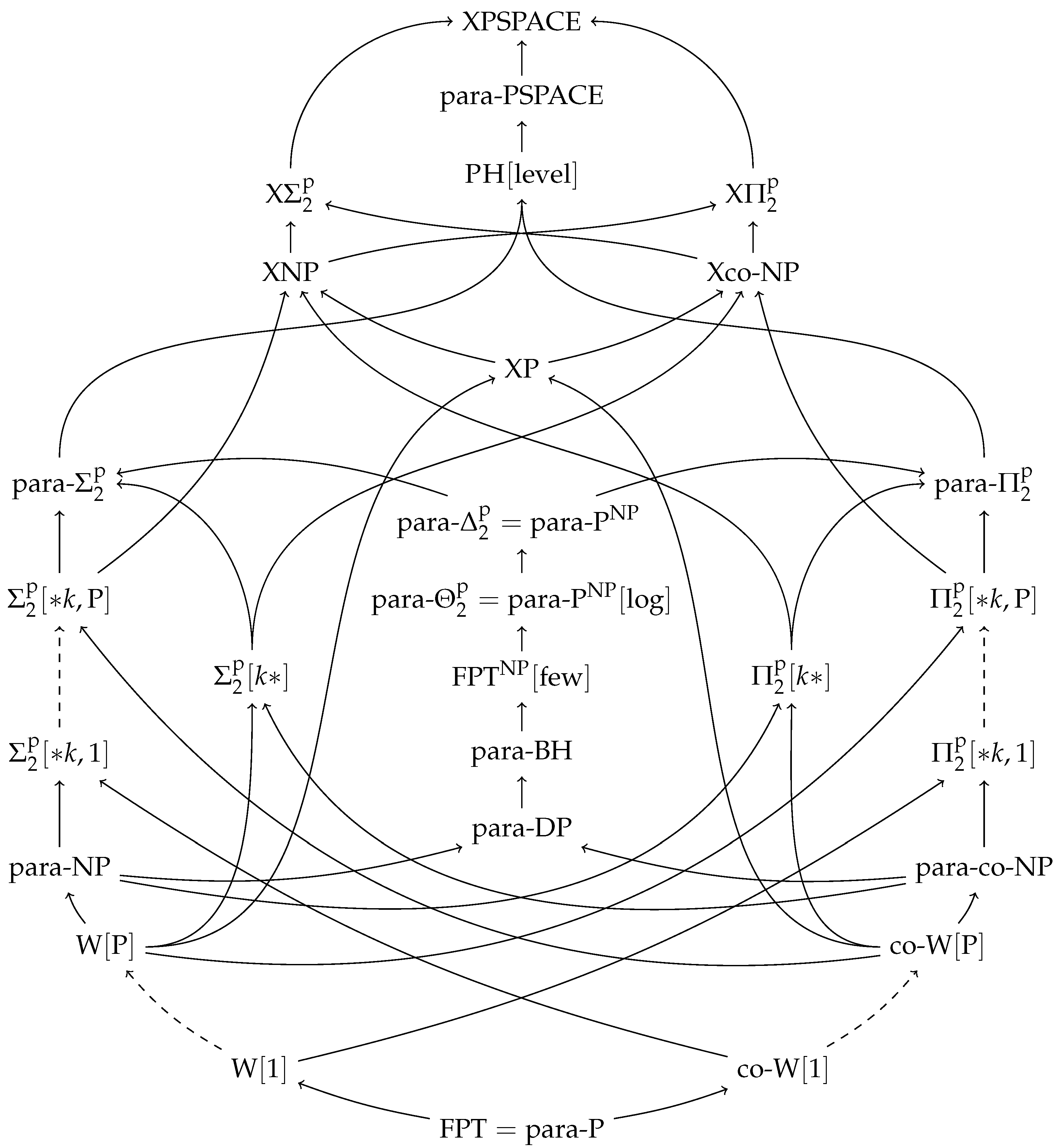
Note that these definitions are entirely analogous to those of the parameterized complexity classes of the W-hierarchy [20]. The following inclusion relations hold between the classes of the $\ast -k$ hierarchy:

$${\Sigma }_2^{\mathrm{p}}[\ast k,1]\subseteq {\Sigma }_2^{\mathrm{p}}[\ast k,2]\subseteq \cdots \subseteq {\Sigma }_2^{\mathrm{p}}[\ast k,\mathrm{SAT}]\subseteq {\Sigma }_2^{\mathrm{p}}[\ast k,\mathrm{P}].$$

(See also Figure 1 for a visual overview of these inclusion relations.)

Figure 1. An overview of parameterized complexity classes up to the second level of the Polynomial Hierarchy, and higher. Dashed lines indicate a hierarchy of classes—e.g., between $\mathrm{W}\left[1\right]$ and $\mathrm{W}\left[\mathrm{P}\right]$ lies the hierarchy $\mathrm{W}\left[1\right]\subseteq \mathrm{W}\left[2\right]\subseteq \cdots \subseteq \mathrm{W}\left[\mathrm{P}\right]$.

Dual to the classical complexity class ${\Sigma }_2^{\mathrm{p}}$ is its co-class ${\Pi }_2^{\mathrm{p}}$, whose canonical complete problem is complementary to the problem QSat${}_2$. Similarly, we can define dual classes for the $k-\ast$ class and for each of the parameterized complexity classes in the $\ast -k$ hierarchy. These co-classes are based on problems complementary to the problems ${\Sigma }_2^{\mathrm{p}}[k\ast ]$-WSat and ${\Sigma }_2^{\mathrm{p}}[\ast k]$-WSat—i.e., these problems have as yes-instances exactly the no-instances of ${\Sigma }_2^{\mathrm{p}}[k\ast ]$-WSat and ${\Sigma }_2^{\mathrm{p}}[\ast k]$-WSat, respectively. Equivalently, these complementary problems can be considered as variants of ${\Sigma }_2^{\mathrm{p}}[k\ast ]$-WSat and ${\Sigma }_2^{\mathrm{p}}[\ast k]$-WSat where the existential and universal quantifiers are swapped, and are therefore denoted with ${\Pi }_2^{\mathrm{p}}[k\ast ]$-WSat and ${\Pi }_2^{\mathrm{p}}[\ast k]$-WSat. We use a similar notation for the dual complexity classes, e.g., we denote co-${\Sigma }_2^{\mathrm{p}}[\ast k,t]$ by ${\Pi }_2^{\mathrm{p}}[\ast k,t]$.

The class ${\Sigma }_2^{\mathrm{p}}[k\ast ]$ includes the class para-$\mathrm{co-NP}$ as a subset, and is contained in the class Xco−NP as a subset. Similarly, each of the classes ${\Sigma }_2^{\mathrm{p}}[\ast k,t]$ include the the class para-NP as a subset, and is contained in the class XNP. Under some common complexity-theoretic assumptions, the class ${\Sigma }_2^{\mathrm{p}}[k\ast ]$ can be separated from para-NP on the one hand, and para-${\Sigma }_2^{\mathrm{p}}$ on the other hand. In particular, assuming that $\mathrm{NP}\ne \mathrm{co-NP}$, it holds that ${\Sigma }_2^{\mathrm{p}}[k\ast ]⊈\mathrm{para-NP}$, that $\mathrm{para-NP}⊈{\Sigma }_2^{\mathrm{p}}[k\ast ]$ and that ${\Sigma }_2^{\mathrm{p}}[k\ast ]⊊\mathrm{para}-{\Sigma }_2^{\mathrm{p}}$ [7,8]. Similarly, the classes ${\Sigma }_2^{\mathrm{p}}[\ast k,t]$ can be separated from para-$\mathrm{co-NP}$ and para-${\Sigma }_2^{\mathrm{p}}$. Assuming that $\mathrm{NP}\ne \mathrm{co-NP}$, it holds that ${\Sigma }_2^{\mathrm{p}}[\ast k,1]⊈\mathrm{para}-\mathrm{co-NP}$, that $\mathrm{para}-\mathrm{co-NP}⊈{\Sigma }_2^{\mathrm{p}}[\ast k,\mathrm{P}]$ and thus in particular that $\mathrm{para}-\mathrm{co-NP}⊈{\Sigma }_2^{\mathrm{p}}[\ast k,1]$, and that ${\Sigma }_2^{\mathrm{p}}[\ast k,\mathrm{P}]⊊\mathrm{para}-{\Sigma }_2^{\mathrm{p}}$ [7,8].

One can also enhance the power of polynomial-time SAT encodings by considering polynomial- time algorithms that can query a SAT solver multiple times—that is, polynomial-time Turing reductions. Such an approach has been shown to be quite effective in practice (see, e.g., [33,34,35]) and extends the scope of SAT solvers to problems in the class ${\Delta }_2^{\mathrm{p}}$, but not to problems that are ${\Sigma }_2^{\mathrm{p}}$-hard or ${\Pi }_2^{\mathrm{p}}$-hard. In addition, here, switching from polynomial-time to fpt-time provides a significant increase in power. The class para-${\Delta }_2^{\mathrm{p}}$ contains all parameterized problems that can be decided by an fpt-algorithm that can query a SAT oracle multiple times—i.e., by an fpt-time Turing reduction to SAT. (One can prove this by following the proof of Theorem 4 in [24] that $\mathrm{FPT}=\mathrm{para}-\mathrm{P}$, with the modification that the algorithms are given access to a SAT oracle.) In addition, one could restrict the number of queries that the algorithm is allowed to make. The class para-${\Theta }_2^{\mathrm{p}}$ consists of all parameterized problems that can be decided by an fpt-algorithm that can query a SAT oracle at most $f\left(k\right)logn$ many times, where k is the parameter value, n is the input size, and f is some computable function. (This statement one can prove by following the proof of Theorem 4 in [24] that $\mathrm{FPT}=\mathrm{para}-\mathrm{P}$, with the modification that the algorithms can query a SAT oracle an amount of times that depends logarithmically on the input size.) Restricting the number of queries even further, we define the parameterized complexity class ${\mathrm{FPT}}^{\mathrm{NP}}\left[\mathrm{few}\right]$ as the class of all parameterized problems that can be decided by an fpt-algorithm that can query a SAT oracle at most $f\left(k\right)$ times, where k is the parameter value and f is some computable function [7,8].

We get the parameterized analogue para-PSPACE of the class PSPACE by using the definition of para-K for $\mathrm{K}=\mathrm{PSPACE}$. Similarly, we can define the parameterized complexity class XPSPACE, consisting of all parameterized problems Q for which there exists a computable function f and an algorithm A that decides whether $(x,k)\in Q$ in space ${\left|x\right|}^{f\left(k\right)}$. We also consider another parameterized variant of PSPACE, which is based on parameterizing the number of quantifier alternations in QSat. An unbounded number of quantifier alternations in this problem results in the class PSPACE, and bounding the number of quantifier alternations by a constant leads to some fixed level of the PH. The parameterized complexity class PH$\left[\mathrm{level}\right]$ is based on bounding the number of quantifier alternations by the problem parameter [7,36]. Formally, we consider the following parameterized problem QSat(level).

QSat(level) Instance: A quantified Boolean formula $\phi =\exists X_1\forall X_2\exists X_3\cdots Q_k{X}_k\psi$, where $Q_k$ is a universal quantifier if k is even and an existential quantifier if k is odd, and where $\psi$ is quantifier-free. Parameter: k. Question: Is $\phi$ true?

The parameterized complexity class PH$\left[\mathrm{level}\right]$ is defined to be the class of all parameterized problems that can be fpt-reduced to QSat(level). We have that $\mathrm{para}-{\Sigma }_2^{\mathrm{p}}\cup \mathrm{para}-{\Pi }_2^{\mathrm{p}}\subseteq \mathrm{PH}\left[\mathrm{level}\right]\subseteq \mathrm{para-PSPACE}$.

An overview of the parameterized complexity classes relevant for this paper can be found in Figure 1.

In the early literature on this topic [6,28,30,37,38,39,40,41], the class ${\Sigma }_2^{\mathrm{p}}[k\ast ]$ appeared under the names ${\exists }^k\forall$ and ${\exists }^k{\forall }^{\ast }$. Similarly, the classes ${\Sigma }_2^{\mathrm{p}}[\ast k,t]$ appeared under the names $\exists {\forall }^k-\mathrm{W}\left[t\right]$ and ${\exists }^{\ast }{\forall }^k-\mathrm{W}\left[t\right]$. In addition, the class ${\mathrm{FPT}}^{\mathrm{NP}}\left[\mathrm{few}\right]$ appeared under the name ${\mathrm{FPT}}^{\mathrm{NP}}\left[f\left(k\right)\right]$.

2.4. Treewidth and Tree Decompositions

We conclude this section with explaining the notions of tree decompositions and treewidth that we use in various places through the paper. For more details on these notions, we refer to textbooks—e.g., [19,20,21,22,23,42].

A tree decomposition of a graph $G=(V,E)$ is a pair $(\mathcal{T},{\left(B_t\right)}_{t\in T})$ where $\mathcal{T}=(T,F)$ is a rooted tree and ${\left(B_t\right)}_{t\in T}$ is a family of subsets of V such that:

• for every $v\in V$, the set $B^{-1}\left(v\right)=\{t\in T:v\in B_t\}$ is nonempty and connected in $\mathcal{T}$; and
• for every edge $\{v,w\}\in E$, there is a $t\in T$ such that $v,w\in B_t$.

The width of the decomposition $(\mathcal{T},{\left(B_t\right)}_{t\in T})$ is the number $max\left\{\right|B_t|:t\in T\}-1$. The treewidth of G is the minimum of the widths of all tree decompositions of G. Let G be a graph and k a nonnegative integer. There is an fpt-algorithm that computes a tree decomposition of G of width k if it exists, and fails otherwise [43]. We call a tree decomposition $(\mathcal{T},{\left(B_t\right)}_{t\in T})$ nice if every node $t\in T$ is of one of the following four types:

• leaf node: t has no children and $|B_t|=1$;
• introduce node: t has one child $t^{\prime }$ and $B_t=B_{t^{\prime }}\cup \left\{v\right\}$ for some vertex $v\notin B_{t^{\prime }}$;
• forget node: t has one child $t^{\prime }$ and $B_t=B_{t^{\prime }}\backslash \left\{v\right\}$ for some vertex $v\in B_{t^{\prime }}$; or
• join node: t has two children $t_1,t_2$ and $B_t=B_{t_1}=B_{t_2}$.

Given any graph G and a tree decomposition of G of width k, a nice tree decomposition of G of width k can be computed in polynomial time [42].

3. Propositional Logic Problems

We start with the quantified circuit satisfiability problems on which the $k-\ast$ and $\ast -k$ hierarchies are based. We present two canonical forms of the problems in the $k-\ast$ hierarchy. For problems in the $\ast -k$ hierarchy, we let $\mathcal{C}$ range over classes of Boolean circuits.

${\Sigma }_2^{\mathrm{p}}[k\ast ]$-WSat($𝒞$) Instance: A Boolean circuit $C\in \mathcal{C}$ over two disjoint sets X and Y of variables, and an integer k. Parameter: k. Question: Does there exist a truth assignment $\alpha$ to X of weight k, such that for all truth assignments $\beta$ to Y the assignment $\alpha \cup \beta$ satisfies C?

Complexity:${\Sigma }_2^{\mathrm{p}}[k\ast ]$-complete [7,8].

${\Sigma }_2^{\mathrm{p}}[k\ast ]$-WSat Instance: A quantified Boolean formula $\varphi =\exists X.\forall Y.\psi$, and an integer k. Parameter: k. Question: Does there exist a truth assignment $\alpha$ to X with weight k, such that $\forall Y.\psi \left[\alpha \right]$ evaluates to true?

Complexity:${\Sigma }_2^{\mathrm{p}}[k\ast ]$-complete [7,8].

${\Sigma }_2^{\mathrm{p}}[\ast k]$-WSat($𝒞$) Instance: A Boolean circuit $C\in \mathcal{C}$ over two disjoint sets X and Y of variables, and an integer k. Parameter: k. Question: Does there exist a truth assignment $\alpha$ to X, such that for all truth assignments $\beta$ to Y of weight k the assignment $\alpha \cup \beta$ satisfies C?

Complexity: ${\Sigma }_2^{\mathrm{p}}[\ast k,t]$-complete when restricted to circuits of weft t, for any $t\ge 1$ (by definition); ${\Sigma }_2^{\mathrm{p}}[\ast k,\mathrm{SAT}]$-complete if $\mathcal{C}=\mathrm{FORM}$ (by definition); ${\Sigma }_2^{\mathrm{p}}[\ast k,\mathrm{P}]$-complete if $\mathcal{C}=\mathrm{CIRC}$ (by definition).

3.1. Weighted Quantified Boolean Satisfiability for the $k-\ast$ Classes

Consider the following variants of ${\Sigma }_2^{\mathrm{p}}[k\ast ]$-WSat, most of which are ${\Sigma }_2^{\mathrm{p}}[k\ast ]$-complete.

${\Sigma }_2^{\mathrm{p}}[k\ast ]$-WSat(3DNF) Instance: A quantified Boolean formula $\varphi =\exists X.\forall Y.\psi$ with $\psi \in 3\mathrm{DNF}$, and an integer k. Parameter: k. Question: Does there exist a truth assignment $\alpha$ to X with weight k, such that $\forall Y.\psi \left[\alpha \right]$ evaluates to true?

Complexity:${\Sigma }_2^{\mathrm{p}}[k\ast ]$-complete [7,8].

${\Sigma }_2^{\mathrm{p}}[k\ast ]$-WSat${}^{\le k}$ Instance: A quantified Boolean formula $\varphi =\exists X.\forall Y.\psi$, and an integer k. Parameter: k. Question: Does there exist an assignment $\alpha$ to X with weight at most k, such that $\forall Y.\psi \left[\alpha \right]$ evaluates to true?

Complexity:${\Sigma }_2^{\mathrm{p}}[k\ast ]$-complete [7,8].

${\Sigma }_2^{\mathrm{p}}[k\ast ]$-WSat${}^{\ge k}$ Instance: A quantified Boolean formula $\varphi =\exists X.\forall Y.\psi$, and an integer k. Parameter: k. Question: Does there exist an assignment $\alpha$ to X with weight at least k, such that $\forall Y.\psi \left[\alpha \right]$ evaluates to true?

Complexity: para-${\Sigma }_2^{\mathrm{p}}$-complete [7].

${\Sigma }_2^{\mathrm{p}}[k\ast ]$-WSat${}^{n-k}$ Instance: A quantified Boolean formula $\varphi =\exists X.\forall Y.\psi$, and an integer k. Parameter: k. Question: Does there exist an assignment $\alpha$ to X with weight $\left|X\right|-k$, such that $\forall Y.\psi \left[\alpha \right]$ evaluates to true?

Complexity:${\Sigma }_2^{\mathrm{p}}[k\ast ]$-complete [7].

3.2. Weighted Quantified Boolean Satisfiability in the $\ast -k$ Hierarchy

Let $d\ge 2$ be an arbitrary constant. Then, the following problem is also ${\Sigma }_2^{\mathrm{p}}[\ast k,1]$-complete.

${\Sigma }_2^{\mathrm{p}}[\ast k]$-WSat(d-DNF) Instance: A quantified Boolean formula $\phi =\exists X.\forall Y.\psi$ with $\psi \in d-\mathrm{DNF}$, and an integer k Parameter: k. Question: Does there exist an assignment $\alpha$ to X, such that for all assignments $\beta$ to Y of weight k the assignment $\alpha \cup \beta$ satisfies $\psi$?

Complexity:${\Sigma }_2^{\mathrm{p}}[\ast k,1]$-complete for any $d\ge 2$ [7,8].

The problem ${\Sigma }_2^{\mathrm{p}}[\ast k]$-WSat(2-DNF) is ${\Sigma }_2^{\mathrm{p}}[\ast k,1]$-hard, even when we restrict the input formula to be anti-monotone in the universal variables, i.e., the universal variables occur only in negative literals [7,8].

Let C be a Boolean circuit with input nodes Z that is in negation normal form, and let $Y\subseteq Z$ be a subset of the input nodes. We say that C is monotone in Y if the only negation nodes that occur in the circuit C act on input nodes in $Z\backslash Y$, i.e., input nodes in Y can appear only positively in the circuit. Similarly, we say that C is anti-monotone in Y if the only nodes that have nodes in Y as input are negation nodes, i.e., all input nodes in Y appear only negatively in the circuit. The following problems are ${\Sigma }_2^{\mathrm{p}}[\ast k,\mathrm{P}]$-complete.

${\Sigma }_2^{\mathrm{p}}[\ast k]$-WSat(-monotone) Instance: A Boolean circuit $C\in \mathrm{CIRC}$ over two disjoint sets X and Y of variables that is in negation normal form and that is monotone in Y, and an integer k. Parameter: k. Question: Does there exist a truth assignment $\alpha$ to X, such that for all truth assignments $\beta$ to Y of weight k the assignment $\alpha \cup \beta$ satisfies C?

Complexity:${\Sigma }_2^{\mathrm{p}}[\ast k,\mathrm{P}]$-complete [7,8].

${\Sigma }_2^{\mathrm{p}}[\ast k]$-WSat(-anti-monotone) Instance: A Boolean circuit $C\in \mathrm{CIRC}$ over two disjoint sets X and Y of variables that is in negation normal form and that is anti-monotone in Y, and an integer k. Parameter: k. Question: Does there exist a truth assignment $\alpha$ to X, such that for all truth assignments $\beta$ to Y of weight k the assignment $\alpha \cup \beta$ satisfies C?

Complexity:${\Sigma }_2^{\mathrm{p}}[\ast k,\mathrm{P}]$-complete [7].

It remains open what the exact parameterized complexity is of ∃-monotone and ∃-anti-monotone variants of ${\Sigma }_2^{\mathrm{p}}[\ast k]$-WSat—i.e., variants of ${\Sigma }_2^{\mathrm{p}}[\ast k]$-WSat that are based on circuits $C\in \mathrm{CIRC}$ over two disjoint sets X and Y of variables that are in negation normal form and that are (anti-)monotone in X. The proofs used to show ${\Sigma }_2^{\mathrm{p}}[\ast k,\mathrm{P}]$-completeness of the ∀-monotone and ∀-anti-monotone variants [7,8] do not immediately carry over to this case.

3.3. Quantified Boolean Satisfiability with Bounded Treewidth

Let $\psi ={\delta }_1\vee \cdots \vee {\delta }_u$ be a DNF formula. For any subset $Z\subseteq \mathrm{Var}\left(\psi \right)$ of variables, we define the incidence graph $\mathrm{IG}(Z,\psi )$ of ψ with respect to Z to be the graph $\mathrm{IG}(Z,\psi )=(V,E)$, where $V=Z\cup \{{\delta }_1,\cdots ,{\delta }_u\}$ and $E=\{\{{\delta }_j,z\}:1\le j\le u\mathrm{and}z\in Z\mathrm{and}z\mathrm{occurs}\mathrm{in}\mathrm{the}\mathrm{clause}{\delta }_j\}$. If $\psi$ is a DNF formula, $Z\subseteq \mathrm{Var}\left(\psi \right)$ is a subset of variables, and $(\mathcal{T},{\left(B_t\right)}_{t\in T})$ is a tree decomposition of $\mathrm{IG}(Z,\psi )$, we let $\mathrm{Var}\left(t\right)$ denote $B_t\cap Z$, for any $t\in T$.

The following parameterized decision problems are variants of QSat${}_2$, where the treewidth of the incidence graph graph for certain subsets of variables is bounded.

QSat${}_2$(itw) Instance: A quantified Boolean formula $\phi =\exists X.\forall Y.\psi$, with $\psi$ in DNF. Parameter: The treewidth of the incidence graph $\mathrm{IG}(X\cup Y,\psi )$ of $\psi$ with respect to $X\cup Y$. Question: Is $\phi$ satisfiable?

Complexity: fixed-parameter tractable [4,5].

QSat${}_2$(∃-itw) Instance: A quantified Boolean formula $\phi =\exists X.\forall Y.\psi$, with $\psi$ in DNF. Parameter: The treewidth of the incidence graph $\mathrm{IG}(X,\psi )$ of $\psi$ with respect to X. Question: Is $\phi$ satisfiable?

Complexity: para-${\Sigma }_2^{\mathrm{p}}$-complete [6,7].

QSat${}_2$(∀-itw) Instance: A quantified Boolean formula $\phi =\exists X.\forall Y.\psi$, with $\psi$ in DNF. Parameter: The treewidth of the incidence graph $\mathrm{IG}(Y,\psi )$ of $\psi$ with respect to Y. Question: Is $\phi$ satisfiable?

Complexity: para-NP-complete [6,7].

The above problems are parameterized by the treewidth of the incidence graph of the formula $\psi$ (with respect to different subsets of variables). Since computing the treewidth of a given graph is NP-hard, it is unlikely that the parameter value can be computed in polynomial time for these problems. Alternatively, one could consider a variant of the problem where a tree decomposition of width k is given as part of the input.

3.4. Other Quantified Boolean Satisfiability

The following parameterized quantified Boolean satisfiability problem is para-NP-complete.

QSat(#∀-vars) Instance: A quantified Boolean formula $\phi$. Parameter: The number of universally quantified variables of $\phi$. Question: Is $\phi$ true?

Complexity: para-NP-complete [6,44,45].

3.5. Minimization for DNF Formulas

Let $\phi$ be a propositional formula in DNF. We say that a set C of literals is an implicant of $\phi$ if all assignments that satisfy ${\bigwedge }_{l\in C}l$ also satisfy $\phi$. Moreover, we say that a DNF formula ${\phi }^{\prime }$ is a term-wise subformula of ${\phi }^{\prime }$ if for all terms $t^{\prime }\in {\phi }^{\prime }$ there exists a term $t\in \phi$ such that $t^{\prime }\subseteq t$. The following parameterized problems are natural parameterizations of problems shown to be ${\Sigma }_2^{\mathrm{p}}$-complete by Umans [46].

Shortest-Implicant-Core(core size) Instance: A DNF formula $\phi$, an implicant C of $\phi$, and an integer k. Parameter: k. Question: Does there exist an implicant $C^{\prime }\subseteq C$ of $\phi$ of size k?

Complexity:${\Sigma }_2^{\mathrm{p}}[k\ast ]$-complete [6,7].

Shortest-Implicant-Core(reduction size) Instance: A DNF formula $\phi$, an implicant C of $\phi$ of size n, and an integer k. Parameter: k. Question: Does there exist an implicant $C^{\prime }\subseteq C$ of $\phi$ of size $n-k$?

Complexity:${\Sigma }_2^{\mathrm{p}}[k\ast ]$-complete [6,7].

DNF-Minimization(reduction size) Instance: A DNF formula $\phi$ of size n, and an integer k. Parameter: k. Question: Does there exist a term-wise subformula ${\phi }^{\prime }$ of $\phi$ of size $n-k$ such that $\phi \equiv {\phi }^{\prime }$?

Complexity:${\Sigma }_2^{\mathrm{p}}[k\ast ]$-complete [6,7].

DNF-Minimization(core size) Instance: A DNF formula $\phi$ of size n, and an integer k. Parameter: k. Question: Does there exist an DNF formula ${\phi }^{\prime }$ of size k, such that $\phi \equiv {\phi }^{\prime }$?

Complexity: para-$\mathrm{co}-\mathrm{NP}$-hard, in ${\mathrm{FPT}}^{\mathrm{NP}}\left[\mathrm{few}\right]$, and in ${\Sigma }_2^{\mathrm{p}}[k\ast ]$ [6,7].

3.6. Sequences of Propositional Formulas

The following problem is related to a Boolean combination of satisfiability checks on a sequence of propositional formulas. This is a parameterized version of the problem ${\mathrm{BH}}_i$-Sat, which is canonical for the different levels of the Boolean Hierarchy (see Section 1). The problem is complete for the class ${\mathrm{FPT}}^{\mathrm{NP}}\left[\mathrm{few}\right]$.

BH-Sat(level) Instance: A positive integer k and a sequence $({\phi }_1,\cdots ,{\phi }_k)$ of propositional formulas. Parameter: k. Question: Is it the case that $({\phi }_1,\cdots ,{\phi }_k)\in$${\mathrm{BH}}_k$-Sat?

Complexity:${\mathrm{FPT}}^{\mathrm{NP}}\left[\mathrm{few}\right]$-complete [7,28,37].

The above problem is used to show the following lower bound result for ${\mathrm{FPT}}^{\mathrm{NP}}\left[\mathrm{few}\right]$-complete problems. No ${\mathrm{FPT}}^{\mathrm{NP}}\left[\mathrm{few}\right]$-hard problem can be decided by an fpt-algorithm that uses only $O\left(1\right)$ many queries to an NP oracle, unless the Polynomial Hierarchy collapses to the third level [18,37].

The next ${\mathrm{FPT}}^{\mathrm{NP}}\left[\mathrm{few}\right]$-complete problem is based on the problem $\mathrm{SAT}-\mathrm{UNSAT}=\{({\phi }_1,{\phi }_2):{\phi }_1\in \mathrm{SAT},{\phi }_2\in \mathrm{UNSAT}\}$.

Bounded-SAT-UNSAT-Disjunction Instance: A family ${({\phi }_i,{\phi }_i^{\prime })}_{i\in \left[k\right]}$ of pairs of propositional formulas. Parameter: k. Question: Is there some $\ell \in \left[k\right]$ such that $({\phi }_{\ell },{\phi }_{\ell }^{\prime })\in \mathrm{SAT}-\mathrm{UNSAT}$?

Complexity:${\mathrm{FPT}}^{\mathrm{NP}}\left[\mathrm{few}\right]$-complete [7,28,37].

3.7. Maximal Models

The following ${\mathrm{FPT}}^{\mathrm{NP}}\left[\mathrm{few}\right]$-complete problems are based on various notions of (local) maximality for models of propositional formulas. Let $\phi$ be a (satisfiable) propositional formula, and let $X\subseteq \mathrm{Var}\left(\phi \right)$ be a subset of variables. Then, a truth assignment $\alpha :\mathrm{Var}\left(\phi \right)\to \{0,1\}$ is an X-maximal model of $\phi$ if (i) $\alpha$ satisfies $\phi$ and (ii) there is no truth assignment $\beta :\mathrm{Var}\left(\phi \right)\to \{0,1\}$ that satisfies $\phi$ and that sets more variables among X to true than $\alpha$. Moreover, take an arbitrary ordering over the variables $X\subseteq \mathrm{Var}\left(\phi \right)$—for the sake of presentation, let $X=\{x_1,\cdots ,x_k\}$ and let the ordering < specify $x_1<\cdots <x_k$. We say that a truth assignment $\alpha :\mathrm{Var}\left(\phi \right)\to \{0,1\}$ is the lexicographically X-maximal model of $\phi$ (with respect to the given ordering) if (i) $\alpha$ satisfies $\phi$ and (ii) each truth assignment $\beta :\mathrm{Var}\left(\phi \right)\to \{0,1\}$ that satisfies $\phi$ (with $\alpha \ne \beta$) has the property that there is some $1\le \ell \le k$ such that $\alpha \left(x_{\ell }\right)=1$ and $\beta \left(x_{\ell }\right)=0$ and for all $1\le {\ell }^{\prime }<\ell$ it holds that $\alpha \left(x_{{\ell }^{\prime }}\right)=\beta \left(x_{{\ell }^{\prime }}\right)$.

Local-Max-Model Instance: A satisfiable propositional formula $\phi$, a subset $X\subseteq \mathrm{Var}\left(\phi \right)$ of variables, and a variable $w\in X$. Parameter:$\left|X\right|$. Question: Is there a X-maximal model of $\phi$ that sets w to true?

Complexity:${\mathrm{FPT}}^{\mathrm{NP}}\left[\mathrm{few}\right]$-complete [7,47].

Local-Lex-Max-Model Instance: A satisfiable propositional formula $\phi$, a subset $X\subseteq \mathrm{Var}\left(\phi \right)$ of variables, and a variable $w\in X$. Parameter:$\left|X\right|$. Question: Is there a lexicographically X-maximal model of $\phi$ that sets w to true?

Complexity:${\mathrm{FPT}}^{\mathrm{NP}}\left[\mathrm{few}\right]$-complete [7]. (The problem Local-Lex-Max-Model isn’t considered explicitly in the literature. ${\mathrm{FPT}}^{\mathrm{NP}}\left[\mathrm{few}\right]$-completeness for this problem follows immediately from proofs in the literature—i.e., Propositions 73 and 74 in [7]).

Odd-Local-Max-Model Instance: A propositional formula $\phi$, and a subset $X\subseteq \mathrm{Var}\left(\phi \right)$ of variables. Parameter:$\left|X\right|$. Question: Do the X-maximal models of $\phi$ set an odd number of variables in X to true?

Complexity:${\mathrm{FPT}}^{\mathrm{NP}}\left[\mathrm{few}\right]$-complete [7].

Odd-Local-Lex-Max-Model Instance: A propositional formula $\phi$, a subset $X\subseteq \mathrm{Var}\left(\phi \right)$ of variables, and an ordering < over the variables in X. Parameter:$\left|X\right|$. Question: Does the lexicographically X-maximal model of $\phi$ (w.r.t. <) set an odd number of variables in X to true?

Complexity:${\mathrm{FPT}}^{\mathrm{NP}}\left[\mathrm{few}\right]$-complete [7].

4. Knowledge Representation and Reasoning Problems

4.1. Disjunctive Answer Set Programming

The following problems from the setting of disjunctive answer set programming (ASP) are based on the notions of disjunctive logic programs and answer sets for such programs (cf. [48,49]). A disjunctive logic program P is a finite set of rules of the form $r=(a_1\vee \cdots \vee a_k\leftarrow$$b_1,\cdots ,b_m,$ $\mathit{not}{c}_1,\cdots ,\mathit{not}{c}_n)$, for $k,m,n\ge 0$, where all $a_i$, $b_j$ and $c_l$ are atoms. For each such rule, $a_1\vee \cdots \vee a_k$ is called the head of the rule, and $b_1,\cdots ,b_m,\mathit{not}{c}_1,\cdots ,\mathit{not}{c}_n$ is called the body of the rule. A rule is called disjunctive if $k>1$, and it is called normal if $k\le 1$ (note that we only call rules with strictly more than one disjunct in the head disjunctive). A rule is called dual-normal if $m\le 1$. A program is called normal if all its rules are normal, it is called negation-free if all its rules are negation-free, and it is called dual-normal if all its rules are dual-normal. We let $\mathrm{At}\left(P\right)$ denote the set of all atoms occurring in P. By literals, we mean atoms a or their negations $\mathit{not}a$. The (Gelfond–Lifschitz) reduct of a program P with respect to a set M of atoms, denoted $P^M$, is the program obtained from P by: (i) removing rules with $\mathit{not}a$ in the body, for each $a\in M$, and (ii) removing literals $\mathit{not}a$ from all other rules [50]. An answer set A of a program P is a subset-minimal model of the reduct $P^A$. One important decision problem is to decide, given a disjunctive logic program P, whether P has an answer set.

We consider various parameterizations of this problem. Two of these are related to atoms that must be part of any answer set of a program P. We identify a subset $\mathrm{Comp}\left(P\right)$ of compulsory atoms, that any answer set must include. Given a program P, we let $\mathrm{Comp}\left(P\right)$ be the smallest set such that: (i) if $(w\leftarrow \mathit{not}w)$ is a rule of P, then $w\in \mathrm{Comp}\left(P\right)$; and (ii) if $(b\leftarrow a_1,\cdots ,a_n)$ is a rule of P, and $a_1,\cdots ,a_n\in \mathrm{Comp}\left(P\right)$, then $b\in \mathrm{Comp}\left(P\right)$. We then let the set $\mathrm{Cont}\left(P\right)$ of contingent atoms be those atoms that occur in P but are not in $\mathrm{Comp}\left(P\right)$. We call a rule contingent if all the atoms that appear in the head are contingent. Another of the parameterizations that we consider is based on the notion of backdoors to normality for disjunctive logic programs. A set B of atoms is a normality-backdoor for a program P if deleting the atoms $b\in B$ from the rules of P results in a normal program. Deciding if a program P has a normality-backdoor of size at most k can be decided in fixed-parameter tractable time [29].

ASP-consistency$(\#\mathrm{cont}.\mathrm{atoms})$ Instance: A disjunctive logic program P. Parameter: The number of contingent atoms of P. Question: Does P have an answer set?

Complexity: para-$\mathrm{co}-\mathrm{NP}$-complete [7,30].

ASP-consistency$(\#\mathrm{cont}.\mathrm{rules})$ Instance: A disjunctive logic program P. Parameter: The number of contingent rules of P. Question: Does P have an answer set?

Complexity:${\Sigma }_2^{\mathrm{p}}[k\ast ]$-complete [7,30].

ASP-consistency$(\#\mathrm{disj}.\mathrm{rules})$ Instance: A disjunctive logic program P. Parameter: The number of disjunctive rules of P. Question: Does P have an answer set?

Complexity:${\Sigma }_2^{\mathrm{p}}[\ast k,\mathrm{P}]$-complete [7,30].

ASP-consistency$(\#\mathrm{dual}-\mathrm{normal}.\mathrm{rules})$ Instance: A disjunctive logic program P. Parameter: The number of rules of P that are dual-normal. Question: Does P have an answer set?

Complexity:${\Sigma }_2^{\mathrm{p}}[\ast k,\mathrm{P}]$-complete [7].

ASP-consistency$\left(\mathrm{str}.\mathrm{norm}.\mathrm{bd}-\mathrm{size}\right)$ Instance: A disjunctive logic program P. Parameter: The size of the smallest normality-backdoor for P. Question: Does P have an answer set?

Complexity: para-NP-complete [29].

ASP-consistency$\left(\max .\mathrm{atom}.\mathrm{occ}.\right)$ Instance: A disjunctive logic program P. Parameter: The maximum number of times that any atom occurs in P. Question: Does P have an answer set?

Complexity: para-${\Sigma }_2^{\mathrm{p}}$-complete [7,30].

4.2. Robust Constraint Satisfaction

The following problem is based on the class of robust constraint satisfaction problems introduced by Gottlob [51] and Abramsky, Gottlob and Kolaitis [52]. These problems are concerned with the question of whether every partial assignment of a particular size can be extended to a full solution, in the setting of constraint satisfaction problems.

A CSP instance N is a triple $(X,D,C)$, where X is a finite set of variables, the domain D is a finite set of values, and C is a finite set of constraints. Each constraint $c\in C$ is a pair $(S,R)$, where $S=\mathrm{Var}\left(c\right)$, the constraint scope, is a finite sequence of distinct variables from X, and R, the constraint relation, is a relation over D whose arity matches the length of S, i.e., $R\subseteq D^r$, where r is the length of S.

Let $N=(X,D,C)$ be a CSP instance. A partial instantiation of N is a mapping $\alpha :X^{\prime }\to D$ defined on some subset $X^{\prime }\subseteq X$. We say that $\alpha$ satisfies a constraint $c=((x_1,\cdots ,x_r),R)\in C$ if $\mathrm{Var}\left(c\right)\subseteq X^{\prime }$ and $(\alpha \left(x_1\right),\cdots ,\alpha \left(x_r\right))\in R$. If $\alpha$ satisfies all constraints of N then it is a solution of N. We say that $\alpha$ violates a constraint $c=((x_1,\cdots ,x_r),R)\in C$ if there is no extension $\beta$ of $\alpha$ defined on $X^{\prime }\cup \mathrm{Var}\left(c\right)$ such that $(\beta \left(x_1\right),\cdots ,\beta \left(x_r\right))\in R$.

Let k be a positive integer. We say that a CSP instance $N=(X,D,C)$ is k-robustly satisfiable if for each instantiation $\alpha :X^{\prime }\to D$ defined on some subset $X^{\prime }\subseteq X$ of k many variables (i.e., $|X^{\prime }|=k$) that does not violate any constraint in C, it holds that $\alpha$ can be extended to a solution for the CSP instance $(X,D,C)$.

Robust-CSP-Sat Instance: A CSP instance $(X,D,C)$, and an integer k. Parameter: k. Question: Is $(X,D,C)$ k-robustly satisfiable?

Complexity:${\Pi }_2^{\mathrm{p}}[k\ast ]$-complete [7,30].

4.3. Abductive Reasoning

The setting of (propositional) abductive reasoning can be formalized as follows. An abduction instance $\mathcal{P}$ consists of a tuple $(V,H,M,T)$, where V is the set of variables, $H\subseteq V$ is the set of hypotheses, $M\subseteq V$ is the set of manifestations, and T is the theory, a formula in CNF over V. It is required that $M\cap H=\varnothing$. A set $S\subseteq H$ is a solution (or explanation) of $\mathcal{P}$ if (i) $T\cup S$ is consistent and (ii) $T\cup S\models M$. One central problem is to decide, given an abduction instance $\mathcal{P}$ and an integer m, whether there exists a solution S of $\mathcal{P}$ of size at most m. This problem is ${\Sigma }_2^{\mathrm{p}}$-complete in general [53].

Abduction$\left(\mathrm{Krom}-\mathrm{bd}-\mathrm{size}\right)$: Input: an abduction instance $\mathcal{P}=(V,H,M,T)$, and a positive integer m. Parameter: The size of the smallest strong 2CNF-backdoor for T. Question: Does there exist a solution S of $\mathcal{P}$ of size at most m?

Complexity: para-NP-complete [31].

Abduction$\left(\mathrm{non}-\mathrm{Krom}-\mathrm{clauses}\right)$: Input: an abduction instance $\mathcal{P}=(V,H,M,T)$, and a positive integer m. Parameter: The number of clauses in T that contains more than 2 literals. Question: Does there exist a solution S of $\mathcal{P}$ of size at most m?

Complexity:${\Sigma }_2^{\mathrm{p}}[\ast k,1]$-complete [7].

Abduction$\left(\mathrm{Horn}-\mathrm{bd}-\mathrm{size}\right)$: Input: an abduction instance $\mathcal{P}=(V,H,M,T)$, and a positive integer m. Parameter: The size of the smallest strong Horn-backdoor for T. Question: Does there exist a solution S of $\mathcal{P}$ of size at most m?

Complexity: para-NP-complete [31].

Abduction$\left(\mathrm{non}-\mathrm{Horn}-\mathrm{clauses}\right)$: Input: an abduction instance $\mathcal{P}=(V,H,M,T)$, and a positive integer m. Parameter: The number of clauses in T that are not Horn. Question: Does there exist a solution S of $\mathcal{P}$ of size at most m?

Complexity:${\Sigma }_2^{\mathrm{p}}[\ast k,\mathrm{P}]$-complete [7].

5. Graph Problems

5.1. Clique Extensions

Let $G=(V,E)$ be a graph. A clique $C\subseteq V$ of G is a subset of vertices that induces a complete subgraph of G, i.e., $\{v,v^{\prime }\}\in E$ for all $v,v^{\prime }\in C$ such that $v\ne v^{\prime }$. The $\mathrm{W}\left[1\right]$-complete problem of determining whether a graph has a clique of size k is an important problem in the W-hierarchy, and is used in many $\mathrm{W}\left[1\right]$-hardness proofs. We consider a related problem that is complete for ${\Pi }_2^{\mathrm{p}}[\ast k,1]$.

Small-Clique-Extension Instance: A graph $G=(V,E)$, a subset $V^{\prime }\subseteq V$, and an integer k. Parameter: k. Question: Is it the case that for each clique $C\subseteq V^{\prime }$, there is some k-clique D of G such that $C\cup D$ is a $\left(\right|C|+k)$-clique?

Complexity:${\Pi }_2^{\mathrm{p}}[\ast k,1]$-complete [7].

5.2. Graph Coloring Extensions

The following problem related to extending colorings to the leaves of a graph to a coloring on the entire graph, is ${\Pi }_2^{\mathrm{p}}$-complete in the most general setting [54].

Let $G=(V,E)$ be a graph. We will denote those vertices v that have degree 1 by leaves. We call a (partial) function $c:V\to \{1,2,3\}$ a 3-coloring (of G). Moreover, we say that a 3-coloring c is proper if c assigns a color to every vertex $v\in V$, and if for each edge $e=\{v_1,v_2\}\in E$ it holds that $c\left(v_1\right)\ne c\left(v_2\right)$. The problem of deciding, given a graph $G=(V,E)$ with n many leaves and an integer m, whether any 3-coloring that assigns a color to exactly m leaves of G (and to no other vertices) can be extended to a proper 3-coloring of G, is ${\Pi }_2^{\mathrm{p}}$-complete [54]. We consider several parameterizations.

3-Coloring-Extension$\left(\mathrm{degree}\right)$ Instance: a graph $G=(V,E)$ with n many leaves, and an integer m. Parameter: the degree of G. Question: can any 3-coloring that assigns a color to exactly m leaves of G (and to no other vertices) be extended to a proper 3-coloring of G?

Complexity: para-${\Pi }_2^{\mathrm{p}}$-complete [7,41].

3-Coloring-Extension$(\#\mathrm{leaves})$ Instance: a graph $G=(V,E)$ with n many leaves, and an integer m. Parameter: n. Question: can any 3-coloring that assigns a color to exactly m leaves of G (and to no other vertices) be extended to a proper 3-coloring of G?

Complexity: para-NP-complete [7,41].

3-Coloring-Extension$(\#\mathrm{col}.\mathrm{leaves})$ Instance: a graph $G=(V,E)$ with n many leaves, and an integer m. Parameter: m. Question: can any 3-coloring that assigns a color to exactly m leaves of G (and to no other vertices) be extended to a proper 3-coloring of G?

Complexity:${\Pi }_2^{\mathrm{p}}[k\ast ]$-complete [7,41].

3-Coloring-Extension$(\#\mathrm{uncol}.\mathrm{leaves})$ Instance: a graph $G=(V,E)$ with n many leaves, and an integer m. Parameter:$n-m$. Question: can any 3-coloring that assigns a color to exactly m leaves of G (and to no other vertices) be extended to a proper 3-coloring of G?

Complexity: para-${\Pi }_2^{\mathrm{p}}$-complete [7,41].

6. Other Problems

6.1. First-Order Logic Model Checking

First-order logic model checking is at the basis of a well-known hardness theory in parameterized complexity theory [22]. The following problem, also based on first-order logic model checking, offers another characterization of the parameterized complexity class ${\Sigma }_2^{\mathrm{p}}[k\ast ]$. We introduce a few notions that we need for defining the model checking perspective on ${\Sigma }_2^{\mathrm{p}}[k\ast ]$. A (relational) vocabulary $\tau$ is a finite set of relation symbols. Each relation symbol R has an arity $\mathrm{arity}\left(R\right)\ge 1$. A structure $\mathcal{A}$ of vocabulary $\tau$, or τ-structure (or simply structure), consists of a set A called the domain and an interpretation $R^{\mathcal{A}}\subseteq A^{\mathrm{arity}\left(R\right)}$ for each relation symbol $R\in \tau$. We use the usual definition of truth of a first-order logic sentence $\phi$ over the vocubulary $\tau$ in a $\tau$-structure $\mathcal{A}$. We let $\mathcal{A}\models \phi$ denote that the sentence $\phi$ is true in structure $\mathcal{A}$.

${\Sigma }_2^{\mathrm{p}}[k\ast ]$-MC Instance: A first-order logic sentence $\phi =\exists x_1,\cdots ,x_k.\forall y_1,\cdots ,y_n.\psi$ over a vocabulary $\tau$, where $\psi$ is quantifier-free, and a finite $\tau$-structure $\mathcal{A}$. Parameter: k. Question: Is it the case that $\mathcal{A}\models \phi$?

Complexity:${\Sigma }_2^{\mathrm{p}}[k\ast ]$-complete [41].

6.2. Quantified Fagin Definability

The W-hierarchy can also be defined by means of Fagin-definable parameterized problems [22], which are based on Fagin’s characterization of NP. We provide an additional characterization of the class ${\Pi }_2^{\mathrm{p}}[k\ast ]$ by means of some parameterized problems that are quantified analogues of Fagin-defined problems.

Let $\tau$ be an arbitrary vocabulary, and let ${\tau }^{\prime }\subseteq \tau$ be a subvocabulary of $\tau$. We say that a $\tau$-structure $\mathcal{A}$ extends a ${\tau }^{\prime }$-structure $\mathcal{B}$ if (i) $\mathcal{A}$ and $\mathcal{B}$ have the same domain, and (ii) $\mathcal{A}$ and $\mathcal{B}$ coincide on the interpretation of all relational symbols in ${\tau }^{\prime }$, i.e., $R^{\mathcal{A}}=R^{\mathcal{B}}$ for all $R\in {\tau }^{\prime }$. We say that $\mathcal{A}$ extends $\mathcal{B}$ with weight k if ${\sum }_{R\in \tau \backslash {\tau }^{\prime }}\left|R^{\mathcal{A}}\right|=k$. Let $\phi$ be a first-order formula over $\tau$ with a free relation variable X of arity s.

We let ${\Pi }_2$ denote the class of all first-order logic formulas of the form $\forall y_1,\cdots ,y_n.\exists x_1,\cdots ,x_m.\psi$, where $\psi$ is quantifier-free. Let $\phi \left(X\right)$ be a first-order logic formula over $\tau$, with a free relation variable X with arity s. Consider the following parameterized problem.

${\Pi }_2^{\mathrm{p}}[k\ast ]{-\mathrm{FD}}_{\phi }^{(\tau ,{\tau }^{\prime })}$ Instance: A ${\tau }^{\prime }$-structure $\mathcal{B}$, and an integer k. Parameter: k. Question: Is it the case that for each $\tau$-structure $\mathcal{A}$ extending $\mathcal{B}$ with weight k, there exists some relation $S\subseteq A^s$ such that $\mathcal{A}\models \phi \left(S\right)$?

Complexity: in ${\Pi }_2^{\mathrm{p}}[k\ast ]$ for each $\phi \left(X\right)$, ${\tau }^{\prime }$ and $\tau$; ${\Pi }_2^{\mathrm{p}}[k\ast ]$-hard for some $\phi \left(X\right)\in {\Pi }_2$, ${\tau }^{\prime }$ and $\tau$ [7].

Note that this means the following. We let T denote the set of all relational vocabularies, and for any $\tau \in T$ we let ${\mathrm{FO}}_{\tau }^X$ denote the set of all first-order logic formulas over the vocabulary $\tau$ with a free relation variable X. We then get the following characterization of ${\Pi }_2^{\mathrm{p}}[k\ast ]$ [7]:

$${\Pi }_2^{\mathrm{p}}[k\ast ]={\left[\{{\Pi }_2^{\mathrm{p}}[k\ast ]{-\mathrm{FD}}_{\phi }^{({\tau }^{\prime },\tau )}:\tau \in T,{\tau }^{\prime }\subseteq \tau ,\phi \in {\mathrm{FO}}_{\tau }^X\}\right]}^{\mathrm{fpt}}.$$

Additionally, the following parameterized problem is hard for ${\Pi }_2^{\mathrm{p}}[\ast k,1]$.

${\Pi }_2^{\mathrm{p}}[\ast k]{-\mathrm{FD}}_{\phi }^{(\tau ,{\tau }^{\prime })}$ Instance: A ${\tau }^{\prime }$-structure $\mathcal{B}$, and an integer k. Parameter: k. Question: Is it the case that for each $\tau$-structure $\mathcal{A}$ extending $\mathcal{B}$, there exists some relation $S\subseteq A^s$ with $\left|S\right|=k$ such that $\mathcal{A}\models \phi \left(S\right)$?

Complexity:${\Pi }_2^{\mathrm{p}}[\ast k,1]$-hard for some $\phi \left(X\right)\in {\Pi }_2$ [7].

6.3. Symbolic Model Checking for Temporal Logics

The following problems are concerned with the task of verifying whether a temporal logic formula is true in a Kripke structure. This task is of importance in the area of software and hardware verification (see, e.g., [55,56]). We consider three different temporal logics: linear-time temporal logic (LTL), computation tree logic (CTL), and CTL${}^{★}$, which is a superset of both LTL and CTL.

Truth of formulas $\phi$ in these logics is defined over Kripke structures $\mathcal{M}$—we write $\mathcal{M}\models \phi$ if $\phi$ is true in $\mathcal{M}$. We consider Kripke structures that are represented symbolically using propositional formulas. Moreover, for each of the logics $\mathcal{L}\in \{\mathrm{LTL},\mathrm{CTL},\mathrm{CTL}{}^{★}\}$, we consider various restricted fragments $\mathcal{L}\backslash$X, $\mathcal{L}\backslash$U and $\mathcal{L}\backslash$U,X, where certain operators are disallowed. For a full description of the syntax and semantics of these logics, how Kripke structures can be represented symbolically and the restricted fragments that we consider, we refer to Appendix A.

In general, the problem of deciding whether a given temporal logic formula $\phi$ is true in a given symbolically represented Kripke structure $\mathcal{M}$ is PSPACE-hard, even when restricted to formulas $\phi$ of constant size [7,36]. We consider a variant of this problem where the Kripke structures have limited recurrence diameter. The recurrence diameter $\mathrm{rd}\left(\mathcal{M}\right)$ of a Kripke structure $\mathcal{M}$ is the length of the longest simple (non-repeating) path in $\mathcal{M}$.

Symbolic-MC${}^{★}\left[\mathcal{L}\right]$ Input: A symbolically represented Kripke structure $\mathcal{M}$, $rd\left(\mathcal{M}\right)$ in unary, and an $\mathcal{L}$ formula $\phi$. Parameter:$\left|\phi \right|$. Question:$\mathcal{M}\models \phi$?

Complexity: para-co-NP-complete if $\mathcal{L}=\mathrm{LTL}\backslash \mathrm{U},\mathrm{X}$ [7,36], PH$\left[\mathrm{level}\right]$-complete if $\mathcal{L}\in \{\mathrm{CTL},\mathrm{CTL}\backslash \mathrm{X},\mathrm{CTL}\backslash \mathrm{U},\mathrm{CTL}\backslash \mathrm{U},\mathrm{X},\mathrm{CTL}{}^{★}\backslash \mathrm{U},\mathrm{X}\}$ [7,36], and para-PSPACE-complete if $\mathcal{L}\in \{\mathrm{CTL}{}^{★},\mathrm{CTL}{}^{★}\backslash \mathrm{X},\mathrm{CTL}{}^{★}\backslash \mathrm{U}\}$ [7,36].

6.4. Judgment Aggregation

The following problems are related to judgment aggregation, in the domain of computational social choice. Judgment aggregation studies procedures that combine individuals’ opinions into a collective group opinion.

An agenda is a finite nonempty set $\Phi =\{{\phi }_1,\cdots ,{\phi }_n,\neg {\phi }_1,\cdots ,\neg {\phi }_n\}$ of formulas that is closed under complementation. A judgment set J for an agenda $\Phi$ is a subset $J\subseteq \Phi$. We call a judgment set J complete if ${\phi }_i\in J$ or $\neg {\phi }_i\in J$ for all formulas ${\phi }_i$, and we call it consistent if there exists an assignment that makes all formulas in J true. Let $\mathcal{J}(\Phi )$ denote the set of all complete and consistent subsets of $\Phi$. We call a sequence $\mathit{J}\in \mathcal{J}{(\Phi )}^n$ of complete and consistent subsets a profile. A (resolute) judgment aggregation procedure for the agenda $\Phi$ and n individuals is a function $F:\mathcal{J}{(\Phi )}^n\to \mathcal{P}(\Phi \backslash \varnothing )\backslash \varnothing$ that returns for each profile $\mathit{J}$ a non-empty set $F\left(\mathit{J}\right)$ of non-empty judgment sets. An example is the majority rule $F^{\mathrm{maj}}$, where $F^{\mathrm{maj}}\left(\mathit{J}\right)=\left\{J^{\ast }\right\}$ and where $\phi \in J^{\ast }$ if and only if $\phi$ occurs in the majority of judgment sets in $\mathit{J}$, for each $\phi \in \Phi$. We call F complete and consistent, if each $J^{\ast }\in F\left(\mathit{J}\right)$ is complete and consistent, respectively, for every $\mathit{J}\in \mathcal{J}{(\Phi )}^n$. For instance, the majority rule $F^{\mathrm{maj}}$ is complete, whenever the number n of individuals is odd. An agenda $\Phi$ is safe with respect to an aggregation procedure F, if F is consistent when applied to profiles of judgment sets over $\Phi$. We say that an agenda $\Phi$ satisfies the median property (MP) if every inconsistent subset of $\Phi$ has itself an inconsistent subset of size at most 2. Safety for the majority rule can be characterized in terms of the median property as follows: an agenda $\Phi$ is safe for the majority rule if and only if $\Phi$ satisfies the MP [57,58]. The problem of deciding whether an agenda satisfies the MP is ${\Pi }_2^{\mathrm{p}}$-complete [57].

Maj-Agenda-Safety$\left(\mathrm{formula}\mathrm{size}\right)$ Instance: an agenda $\Phi$. Parameter:$\ell =max\left\{\right|\phi |:\phi \in \Phi \}$. Question: Is $\Phi$ safe for the majority rule?

Complexity: para-${\Pi }_2^{\mathrm{p}}$-complete [7,37].

Maj-Agenda-Safety$\left(\mathrm{degree}\right)$ Instance: an agenda $\Phi$ containing only CNF formulas. Parameter: The degree d of $\Phi$. Question: Is $\Phi$ safe for the majority rule?

Complexity: para-${\Pi }_2^{\mathrm{p}}$-complete [7,37].

Maj-Agenda-Safety$(\mathrm{degree}+\mathrm{formula}\mathrm{size})$ Instance: an agenda $\Phi$ containing only CNF formulas, where $\ell =max\left\{\right|\phi |:\phi \in B(\Phi \left)\right\}$, and where d is the degree of $\Phi$. Parameter:$\ell +d$. Question: Is $\Phi$ safe for the majority rule?

Complexity: para-${\Pi }_2^{\mathrm{p}}$-complete [7,37].

The above three parameterized problems remain para-${\Pi }_2^{\mathrm{p}}$-hard even when restricted to agendas based on formulas that are Horn formulas containing only clauses of size at most 2 [7,37].

Maj-Agenda-Safety$\left(\mathrm{agenda}\mathrm{size}\right)$ Instance: an agenda $\Phi$. Parameter:$|\Phi |$. Question: Is $\Phi$ safe for the majority rule?

Complexity:${\mathrm{FPT}}^{\mathrm{NP}}\left[\mathrm{few}\right]$-complete [7,37].

Moreover, the following upper and lower bounds on the number of oracle queries are known for the above problem. Maj-Agenda-Safety$\left(\mathrm{agenda}\mathrm{size}\right)$ can be decided in fpt-time using $2^{O\left(k\right)}$ queries to an NP oracle, where $k=|\Phi |$ [7,37]. In addition, there is no fpt-algorithm that decides Maj-Agenda-Safety$\left(\mathrm{agenda}\mathrm{size}\right)$ using $o(logk)$ queries to an NP oracle, unless the Polynomial Hierarchy collapses [7,37].

Maj-Agenda-Safety$\left(\mathrm{counterexample}\mathrm{size}\right)$ Instance: an agenda $\Phi$, and an integer k. Parameter: k. Question: Does every inconsistent subset ${\Phi }^{\prime }$ of $\Phi$ of size k have itself an inconsistent subset of size at most 2?

Complexity:${\Pi }_2^{\mathrm{p}}[k\ast ]$-hard [7,37].

Let $\Phi =\{{\phi }_1,\cdots ,{\phi }_m,\neg {\phi }_1,\cdots ,\neg {\phi }_m\}$ be an agenda, where each ${\phi }_i$ is a CNF formula. We define the following graphs that are intended to capture the interaction between formulas in $\Phi$. The formula primal graph of $\Phi$ has as vertices the variables $\mathrm{Var}(\Phi )$ occurring in the agenda, and two variables are connected by an edge if there exists a formula ${\phi }_i$ in which they both occur. The formula incidence graph of $\Phi$ is a bipartite graph whose vertices consist of (1) the variables $\mathrm{Var}(\Phi )$ occurring in the agenda and (2) the formulas ${\phi }_i\in \Phi$. A variable $x\in \mathrm{Var}(\Phi )$ is connected by an edge with a formula ${\phi }_i\in \Phi$ if x occurs in ${\phi }_i$, i.e., $x\in \mathrm{Var}\left({\phi }_i\right)$. The clausal primal graph of $\Phi$ has as vertices the variables $\mathrm{Var}(\Phi )$ occurring in the agenda, and two variables are connected by an edge if there exists a formula ${\phi }_i$ and a clause $c\in {\phi }_i$ in which they both occur. The clausal incidence graph of $\Phi$ is a bipartite graph whose vertices consist of (1) the variables $\mathrm{Var}(\Phi )$ occurring in the agenda and (2) the clauses c occurring in formulas ${\phi }_i\in \Phi$. A variable $x\in \mathrm{Var}(\Phi )$ is connected by an edge with a clause c of the formula ${\phi }_i\in \Phi$ if x occurs in c, i.e., $x\in \mathrm{Var}\left(c\right)$. Consider the following parameterizations of the problem Maj-Agenda-Safety.

Maj-Agenda-Safety$\left(\mathrm{f}-\mathrm{tw}\right)$ Instance: an agenda $\Phi$ containing only CNF formulas. Parameter: The treewidth of the formula primal graph of $\Phi$. Question: Is $\Phi$ safe for the majority rule?

Complexity: fixed-parameter tractable [7,37].

Maj-Agenda-Safety$\left(\mathrm{f}-\mathrm{tw}{}^{\ast }\right)$ Instance: an agenda $\Phi$ containing only CNF formulas. Parameter: The treewidth of the formula incidence graph of $\Phi$. Question: Is $\Phi$ safe for the majority rule?

Complexity: para-${\Pi }_2^{\mathrm{p}}$-complete [7,37].

Maj-Agenda-Safety$\left(\mathrm{c}-\mathrm{tw}\right)$ Instance: an agenda $\Phi$ containing only CNF formulas. Parameter: The treewidth of the clausal primal graph of $\Phi$. Question: Is $\Phi$ safe for the majority rule?

Complexity: para-$\mathrm{co}-\mathrm{NP}$-complete [7,37].

Maj-Agenda-Safety$\left(\mathrm{c}-\mathrm{tw}{}^{\ast }\right)$ Instance: an agenda $\Phi$ containing only CNF formulas. Parameter: The treewidth of the clausal incidence graph of $\Phi$. Question: Is $\Phi$ safe for the majority rule?

Complexity: para-$\mathrm{co}-\mathrm{NP}$-complete [7,37].

6.5. Planning

The following parameterized problems are related to planning in the face of uncertainty. We begin by describing the framework of SAS${}^{+}$ planning (see, e.g., [59]). Let $V=\{v_1,\dots ,v_n\}$ be a finite set of variables over a finite domain D. Furthermore, let $D^{+}=D\cup \left\{\mathbf{u}\right\}$, where $\mathbf{u}$ is a special undefined value not present in D. Then $D^n$ is the set of total states and ${\left(D^{+}\right)}^n$ is the set of partial states over V and D. Intuitively, a state $(d_1,\cdots ,d_n)\in D^n$ corresponds to an assignment that assigns to each variable $v_i\in V$ the value $d_i\in D$, and a partial state corresponds to a partial assignment that assigns a value to some variables $v_i\in V$. Clearly, $D^n\subseteq {\left(D^{+}\right)}^n$—that is, each total state is also a partial state. Let $(d_1,\cdots ,d_n)=s\in {\left(D^{+}\right)}^n$ be a state. Then, the value of a variable $v_i$ in state s is denoted by $s\left[v_i\right]=d_i$.

An SAS${}^{+}$ instance is a tuple $\mathbb{P}=(V,D,A,I,G)$, where V is a set of variables, D is a domain, A is a set of actions, $I\in D^n$ is the initial state and $G\in {\left(D^{+}\right)}^n$ is the (partial) goal state. Each action $a\in A$ has a precondition $\mathsf{pre}\left(a\right)\in {\left(D^{+}\right)}^n$ and an effect $\mathsf{eff}\left(a\right)\in {\left(D^{+}\right)}^n$.

We will frequently use the convention that a variable has the value $\mathbf{u}$ in a precondition/effect unless a value is explicitly specified. Furthermore, by a slight abuse of notation, we denote actions and partial states such as preconditions, effects, and goals as follows. Let $a\in A$ be an action, and let $\{p_1,\cdots ,p_m\}\subseteq V$ be the set of variables that are not assigned by $\mathsf{pre}\left(a\right)$ to the value $\mathbf{u}$—that is, $\{v\in V:\mathsf{pre}\left(a\right)\left[v\right]\ne \mathbf{u}\}=\{p_1,\cdots ,p_m\}$. Moreover, suppose that $\mathsf{pre}\left(a\right)\left[p_1\right]=d_1,\dots ,\mathsf{pre}\left(a\right)\left[p_m\right]=d_m$. Then, we denote the precondition $\mathsf{pre}\left(a\right)$ by $\mathsf{pre}\left(a\right)=\{p_1\mapsto d_1,\dots ,p_m\mapsto d_m\}$. In particular, if $\mathsf{pre}\left(a\right)$ is the partial state such that $\mathsf{pre}\left(a\right)\left[v\right]=\mathbf{u}$ for each $v\in V$, we denote $\mathsf{pre}\left(a\right)$ by ∅. We use a similar notation for effects. Let a be the action with $\mathsf{pre}\left(a\right)=\{p_1\mapsto d_1,\dots ,p_m\mapsto d_m\}$ and $\mathsf{eff}\left(a\right)=\{e_1\mapsto d_1^{\prime },\dots ,e_{\ell }\mapsto d_{\ell }^{\prime }\}$. We then use the notation $a:\{p_1\mapsto d_1,\dots ,p_m\mapsto d_m\}\to \{e_1\mapsto d_1^{\prime },\dots ,e_{m^{\prime }}\mapsto d_{m^{\prime }}^{\prime }\}$ to describe the action a.

Let $a\in A$ be an action and $s\in D^n$ be a state. Then, a is valid in s if for all $v\in V$, either $\mathsf{pre}\left(a\right)\left[v\right]=s\left[v\right]$ or $\mathsf{pre}\left(a\right)\left[v\right]=\mathbf{u}$. The result of a in s is the state $t\in D^n$ defined as follows. For all $v\in V$, $t\left[v\right]=\mathsf{eff}\left(a\right)\left[v\right]$ if $\mathsf{eff}\left(a\right)\left[v\right]\ne \mathbf{u}$ and $t\left[v\right]=s\left[v\right]$ otherwise. Let $s_0,s_{\ell }\in D^n$ and let $\omega =(a_1,\dots ,a_{\ell })$ be a sequence of actions (of length ℓ). We say that $\omega$ is a plan from $s_0$ to $s_{\ell }$ if either (i) $\omega$ is the empty sequence (and $\ell =0$, and thus $s_0=s_{\ell }$), or (ii) there are states $s_1,\dots ,s_{\ell -1}\in D^n$ such that for each $i\in [\ell ]$, $a_i$ is valid in $s_{i-1}$ and $s_i$ is the result of $a_i$ in $s_{i-1}$. A state $s\in D^n$ is a goal state if for all $v\in V$, either $G\left[v\right]=s\left[v\right]$ or $G\left[v\right]=\mathbf{u}$. An action sequence $\omega$ is a plan for $\mathbb{P}$ if $\omega$ is a plan from I to a goal state.

We also allow actions to have conditional effects (see, e.g., [60]). A conditional effect is of the form $s▹t$, where $s,t\in {\left(D^{+}\right)}^n$ are partial states. Intuitively, such a conditional effect ensures that the variable assignment t is only applied if the condition s is satisfied. When allowing conditional effects, the effect of an action is not a partial state $\mathsf{eff}\left(a\right)\in {\left(D^{+}\right)}^n$, but a set $\mathsf{eff}\left(a\right)=\{s_1▹t_1,\cdots ,s_{\ell }▹t_{\ell }\}$ of conditional effects. (For the sake of simplicity, we assume that the partial states $t_1,\cdots ,t_{\ell }$ are non-conflicting—that is, there exist no $v\in V$ and no $i_1,i_2\in [\ell ]$ with $i_1<i_2$ such that $\mathbf{u}\ne t_{i_1}\left[v\right]\ne t_{i_2}\left[v\right]\ne \mathbf{u}$.) The result of an action a with $\mathsf{eff}\left(a\right)=\{s_1▹t_1,\cdots ,s_{\ell }▹t_{\ell }\}$ in a state s (in which a is valid) is the state $t\in D^n$ that is defined as follows. For all $v\in V$, $t\left[v\right]=t_i\left[v\right]$ if there exists some $i\in [\ell ]$ such that $s_i$ is satisfied in s and $t_i\left[v\right]\ne \mathbf{u}$, and $t\left[v\right]=s\left[v\right]$ otherwise.

For the parameterized planning problems that we consider, in addition to the variables V, we consider a set $V_u$ of $n^{\prime }$ variables—constituting an uncertain planning instance $\mathbb{P}=(V,V_u,D,A,I,G)$. Intuitively, the value of the variables in $V_u$ in the initial state is unknown. The question is whether there exists an action sequence $\omega$ such that, for each state $I_0\in D^{n+n^{\prime }}$ that extends I—that is, $I_0\left[v\right]=I\left[v\right]$ for each $v\in V$—it holds that $\omega$ is a plan for the SAS${}^{+}$ instance $(V\cup V_u,D,A,I_0,G)$. If there exists such an action sequence $\omega$, we say that $\omega$ is a plan that works for each complete initial state $I_0$ that extends I.

Bounded-Uncertain-Planning Instance: an uncertain planning instance $\mathbb{P}=(V,V_u,D,A,I,G)$, and an integer k. Parameter: k. Question: Is there a plan of length k for $\mathbb{P}$ that works for each complete initial state $I_0$ that extends I?

Complexity:${\Sigma }_2^{\mathrm{p}}[k\ast ]$-complete [7,39].

Polynomial-Planning$\left(\mathrm{bounded}-\mathrm{deviation}\right)$ Instance: an uncertain planning instance $\mathbb{P}=(V,V_u,D,A,I,G)$, an integer d, and an integer u given in unary. Parameter: d. Question: Is there a plan for $\mathbb{P}$ of length $\le u$ that works for each complete initial state $I_0$ that extends I and for which at most d unknown variables deviate from the base value?

Complexity:${\Sigma }_2^{\mathrm{p}}[\ast k,\mathrm{P}]$-complete [7,39].

6.6. Turing Machine Halting

The following problems are related to alternating Turing machines (ATMs), possibly with multiple tapes. ATMs are nondeterministic Turing machines where the states are divided into existential and universal states, and where each configuration of the machine is called existential or universal according to the state that the machine is in. A run $\rho$ of the ATM $\mathbb{M}$ on an input x is a tree whose nodes correspond to configurations of $\mathbb{M}$ in such a way that (1) for each non-root node v of the tree with parent node $v^{\prime }$, the machine $\mathbb{M}$ can transition from the configuration corresponding to $v^{\prime }$ to the configuration corresponding to v, (2) the root node corresponds to the initial configuration of $\mathbb{M}$, and (3) each leaf node corresponds to a halting configuration. A computation path in a run of $\mathbb{M}$ is a root-to-leaf path in the run. Moreover, the nodes of a run $\rho$ are labelled accepting or rejecting, according to the following definition. A leaf of $\rho$ is labelled accepting if the configuration corresponding to it is an accepting configuration, and the leaf is labelled rejecting if it is a rejecting configuration. A non-leaf node of $\rho$ that corresponds to an existential configuration is labelled accepting if at least one of its children is labelled accepting. A non-leaf node of $\rho$ that corresponds to a universal configuration is labelled accepting if all of its children are labelled accepting. An ATM $\mathbb{M}$ is 2-alternating if for each input x, each computation path in the run of $\mathbb{M}$ on input x switches at most once from an existential configuration to a universal configuration, or vice versa. For more details on the terminology, we refer to the work of De Haan and Szeider [8,41] and to the work of Flum and Grohe—Appendix A.1 in [22].

We consider the following restrictions on ATMs. An $\exists \forall$-Turing machine (or simply $\exists \forall$-machine) is a 2-alternating ATM, where the initial state is an existential state. Let $\ell ,t\ge 1$ be positive integers. We say that an $\exists \forall$-machine $\mathbb{M}$ halts (on the empty string) with existential cost ℓ and universal cost t if: (1) there is an accepting run of $\mathbb{M}$ with the empty input $ϵ$, and (2) each computation path of $\mathbb{M}$ contains at most ℓ existential configurations and at most t universal configurations. The following problem, where the number of Turing machine tapes is given as part of the input, is ${\Sigma }_2^{\mathrm{p}}[k\ast ]$-complete.

${\Sigma }_2^{\mathrm{p}}[k\ast ]$-TM-halt*. Instance: Positive integers $m,k,t\ge 1$, and an $\exists \forall$-machine $\mathbb{M}$ with m tapes. Parameter: k. Question: Does $\mathbb{M}$ halt on the empty string with existential cost k and universal cost t?

Complexity:${\Sigma }_2^{\mathrm{p}}[k\ast ]$-complete [7,8].

Let $m\ge 1$ be a constant integer. Then, the following parameterized decision problem, where the number of Turing machine tapes is fixed, is also ${\Sigma }_2^{\mathrm{p}}[k\ast ]$-complete.

${\Sigma }_2^{\mathrm{p}}[k\ast ]$-TM-haltm. Instance: Positive integers $k,t\ge 1$, and an $\exists \forall$-machine $\mathbb{M}$ with m tapes. Parameter: k. Question: Does $\mathbb{M}$ halt on the empty string with existential cost k and universal cost t?

Complexity:${\Sigma }_2^{\mathrm{p}}[k\ast ]$-complete [7,8].

In addition, the parameterized complexity class ${\Sigma }_2^{\mathrm{p}}[k\ast ]$ can also be characterized by means of alternating Turing machines in the following way. Let P be a parameterized problem. An ${\Sigma }_2^{\mathrm{p}}[k\ast ]$-machine for P is a $\exists \forall$-machine $\mathbb{M}$ such that there exists a computable function f and a polynomial p such that: (1) $\mathbb{M}$ decides P in time $f\left(k\right)·p\left(\right|x\left|\right)$; and (2) for all instances $(x,k)$ of P and each computation path R of $\mathbb{M}$ with input $(x,k)$, at most $f\left(k\right)·log\left|x\right|$ of the existential configurations of R are nondeterministic. We say that a parameterized problem P is decided by some ${\Sigma }_2^{\mathrm{p}}[k\ast ]$-machine if there exists a ${\Sigma }_2^{\mathrm{p}}[k\ast ]$-machine for P. Then, ${\Sigma }_2^{\mathrm{p}}[k\ast ]$ is exactly the class of parameterized decision problems that are decided by some ${\Sigma }_2^{\mathrm{p}}[k\ast ]$-machine [7,8].

7. Conclusions

In this paper, we provided a list of parameterized problems that are based on problems at higher levels of the Polynomial Hierarchy, together with a complexity classification indicating whether they allow a (many-to-one or Turing) fpt-reduction to SAT or not. These complexity classifications are based in part on recently developed parameterized complexity classes—e.g., ${\Sigma }_2^{\mathrm{p}}[k\ast ]$ and ${\Sigma }_2^{\mathrm{p}}[\ast k,\mathrm{P}]$ [7,8], ${\mathrm{FPT}}^{\mathrm{NP}}\left[\mathrm{few}\right]$ [6,7] and PH$\left[\mathrm{level}\right]$ [7,36]. The problems that we considered are related to propositional logic, quantified Boolean satisfiability, disjunctive answer set programming, constraint satisfaction, (propositional) abductive reasoning, cliques, graph coloring, first-order logic model checking, temporal logic model checking, judgment aggregation, planning, and (alternating) Turing machines.

References

- Vardi, M.Y. Boolean satisfiability: Theory and engineering. Commun. ACM 2014, 57, 5. [Google Scholar] [CrossRef]
- Stockmeyer, L.J. The polynomial-time hierarchy. Theor. Comput. Sci. 1976, 3, 1–22. [Google Scholar] [CrossRef]
- Wrathall, C. Complete Sets and the Polynomial-Time Hierarchy. Theor. Comput. Sci. 1976, 3, 23–33. [Google Scholar] [CrossRef]
- Chen, H. Quantified Constraint Satisfaction and Bounded Treewidth. In Proceedings of the 16th European Conference on Artificial Intelligence (ECAI 2004), Valencia, Spain, 22–27 August 2004; pp. 161–165. [Google Scholar]
- Feder, T.; Kolaitis, P.G. Closures and dichotomies for quantified constraints. In Electronic Colloquium on Computational Complexity (ECCC); Technical Report TR06-160; Weizmann Institute of Science: Rehovot, Israel, 2006. [Google Scholar]
- De Haan, R.; Szeider, S. Fixed-parameter tractable reductions to SAT. In Proceedings of the 17th International Symposium on the Theory and Applications of Satisfiability Testing (SAT 2014), Vienna, Austria, 14–17 July 2014; Egly, U., Sinz, C., Eds.; Springer: Berlin, Germany, 2014; Volume 8561, pp. 85–102. [Google Scholar]
- De Haan, R. Parameterized Complexity in the Polynomial Hierarchy. Ph.D. Thesis, Technische Universität Wien, Vienna, Austria, 2016. [Google Scholar]
- De Haan, R.; Szeider, S. Parameterized complexity classes beyond para-NP. J. Comput. Syst. Sci. 2017, 87, 16–57. [Google Scholar] [CrossRef]
- Schaefer, M.; Umans, C. Completeness in the Polynomial-Time hierarchy: A Compendium. SIGACT News 2002, 33, 32–49. [Google Scholar]
- Cesati, M. Compendium of Parameterized Problems. Available online: http://cesati.sprg.uniroma2.it/research/compendium/ (accessed on 4 September 2019).
- Arora, S.; Barak, B. Computational Complexity—A Modern Approach; Cambridge University Press: Cambridge, UK, 2009; pp. I–XXIV, 1–579. [Google Scholar]
- Papadimitriou, C.H. Computational Complexity; Addison-Wesley: Boston, MA, USA, 1994. [Google Scholar]
- Meyer, A.R.; Stockmeyer, L.J. The Equivalence Problem for Regular Expressions with Squaring Requires Exponential Space. In Proceedings of the 13th Annual Symposium on Switching & Automata Theory (SWAT), College Park, MD, USA, 25–27 October 1972; pp. 125–129. [Google Scholar]
- Hemachandra, L.A. The strong exponential hierarchy collapses. J. Comput. Syst. Sci. 1989, 39, 299–322. [Google Scholar] [CrossRef]
- Buss, S.R.; Hay, L. On truth-table reducibility to SAT. Inf. Comput. 1991, 91, 86–102. [Google Scholar] [CrossRef]
- Cai, J.; Gundermann, T.; Hartmanis, J.; Hemachandra, L.A.; Sewelson, V.; Wagner, K.W.; Wechsung, G. The Boolean Hierarchy I: Structural Properties. SIAM J. Comput. 1988, 17, 1232–1252. [Google Scholar] [CrossRef]
- Chang, R.; Kadin, J. The Boolean Hierarchy and the Polynomial Hierarchy: A Closer Connection. SIAM J. Comput. 1993, 25, 169–178. [Google Scholar]
- Kadin, J. The Polynomial Time Hierarchy Collapses if the Boolean Hierarchy Collapses. SIAM J. Comput. 1988, 17, 1263–1282. [Google Scholar] [CrossRef]
- Cygan, M.; Fomin, F.V.; Kowalik, L.; Lokshtanov, D.; Marx, D.; Pilipczuk, M.; Pilipczuk, M.; Saurabh, S. Parameterized Algorithms; Springer: Berlin, Germany, 2015. [Google Scholar]
- Downey, R.G.; Fellows, M.R. Parameterized Complexity. In Monographs in Computer Science; Springer: New York, NY, USA, 1999. [Google Scholar]
- Downey, R.G.; Fellows, M.R. Texts in Computer Science. Fundamentals of Parameterized Complexity; Springer: Berlin, Germany, 2013. [Google Scholar]
- Flum, J.; Grohe, M. Parameterized Complexity Theory. In Texts in Theoretical Computer Science. An EATCS Series; Springer: Berlin, Germany, 2006; Volume XIV. [Google Scholar]
- Niedermeier, R. Invitation to Fixed-Parameter Algorithms. In Oxford Lecture Series in Mathematics and Its Applications; Oxford University Press: Oxford, UK, 2006. [Google Scholar]
- Flum, J.; Grohe, M. Describing parameterized complexity classes. Inf. Comput. 2003, 187, 291–319. [Google Scholar] [CrossRef]
- Cook, S.A. The Complexity of Theorem-Proving Procedures. In Proceedings of the Third Annual ACM Symposium on Theory of Computing, Shaker Heights, OH, USA, 3–5 May 1971; pp. 151–158. [Google Scholar]
- Levin, L. Universal sequential search problems. Probl. Inf. Transm. 1973, 9, 265–266. [Google Scholar]
- Prestwich, S.D. CNF Encodings. In Handbook of Satisfiability; Biere, A., Heule, M., van Maaren, H., Walsh, T., Eds.; IOS Press: Amsterdam, The Netherlands, 2009; pp. 75–97. [Google Scholar]
- Endriss, U.; De Haan, R.; Szeider, S. Parameterized Complexity Results for Agenda Safety in Judgment Aggregation. In Proceedings of the 14th International Conference on Autonomous Agents and Multiagent Systems (AAMAS 2015), Istanbul, Turkey, 4–8 May 2015. [Google Scholar]
- Fichte, J.K.; Szeider, S. Backdoors to Normality for Disjunctive Logic Programs. ACM Trans. Comput. Log. 2015, 17, 7:1–7:23. [Google Scholar] [CrossRef]
- De Haan, R.; Szeider, S. The Parameterized Complexity of Reasoning Problems Beyond NP. In Proceedings of the Fourteenth International Conference on the Principles of Knowledge Representation and Reasoning (KR 2014), Vienna, Austria, 20–24 July 2014; Baral, C., De Giacomo, G., Eiter, T., Eds.; AAAI Press: Palo Alto, CA, USA, 2014. [Google Scholar]
- Pfandler, A.; Rümmele, S.; Szeider, S. Backdoors to Abduction. In Proceedings of the 23rd International Joint Conference on Artificial Intelligence (IJCAI 2013), Beijing, China, 3–9 August 2013; Rossi, F., Ed.; AAAI Press: Palo Alto, CA, USA, 2013. [Google Scholar]
- Tseitin, G.S. Complexity of a Derivation in the Propositional Calculus. Zap. Nauchn. Sem. Leningrad Otd. Mat. Inst. Akad. Nauk SSSR 1968, 8, 23–41. [Google Scholar]
- Belov, A.; Lynce, I.; Marques-Silva, J. Towards efficient MUS extraction. AI Commun. 2012, 25, 97–116. [Google Scholar]
- Dvořák, W.; Järvisalo, M.; Wallner, J.P.; Woltran, S. Complexity-sensitive decision procedures for abstract argumentation. Artif. Intell. 2014, 206, 53–78. [Google Scholar] [CrossRef]
- Marques-Silva, J.; Janota, M.; Belov, A. Minimal Sets over Monotone Predicates in Boolean Formulae. In Proceedings of the 25th International Conference Computer Aided Verification (CAV 2013), Saint Petersburg, Russia, 13–19 July 2013; Sharygina, N., Veith, H., Eds.; Springer: Berlin, Germany, 2013; Volume 8044, pp. 592–607. [Google Scholar]
- De Haan, R.; Szeider, S. Parameterized Complexity Results for Symbolic Model Checking of Temporal Logics. In Proceedings of the Fifteenth International Conference on the Principles of Knowledge Representation and Reasoning (KR 2016), Cape Town, South Africa, 25–29 April 2016; pp. 453–462. [Google Scholar]
- Endriss, U.; De Haan, R.; Szeider, S. Parameterized Complexity Results for Agenda Safety in Judgment Aggregation. In Proceedings of the 5th International Workshop on Computational Social Choice (COMSOC-2014), Istanbul, Turkey, 4–8 May 2014. [Google Scholar]
- De Haan, R. An Overview of Non-Uniform Parameterized Complexity. In Electronic Colloquium on Computational Complexity (ECCC); Technical Report TR15-130; Weizmann Institute of Science: Rehovot, Israel, 2015. [Google Scholar]
- De Haan, R.; Kronegger, M.; Pfandler, A. Fixed-parameter Tractable Reductions to SAT for Planning. In Proceedings of the 24th International Joint Conference on Artificial Intelligence (IJCAI 2015), Buenos Aires, Argentina, 25–31 July 2015. [Google Scholar]
- De Haan, R.; Szeider, S. Compendium of Parameterized Problems at Higher Levels of the Polynomial Hierarchy. In Electronic Colloquium on Computational Complexity (ECCC); Technical Report TR14–143; Weizmann Institute of Science: Rehovot, Israel, 2014. [Google Scholar]
- De Haan, R.; Szeider, S. Machine Characterizations for Parameterized Complexity Classes beyond para-NP. In Proceedings of the 41st Conference on Current Trends in Theory and Practice of Computer Science (SOFSEM 2015), Pec pod Sněžkou, Czech Republic, 24–29 January 2015; Springer: Berlin, Germany, 2015; Volume 8939. [Google Scholar]
- Kloks, T. Treewidth: Computations and Approximations; Springer: Berlin, Germany, 1994. [Google Scholar]
- Bodlaender, H.L. A linear-time algorithm for finding tree-decompositions of small treewidth. SIAM J. Comput. 1996, 25, 1305–1317. [Google Scholar] [CrossRef]
- Ayari, A.; Basin, D.A. QUBOS: Deciding Quantified Boolean Logic Using Propositional Satisfiability Solvers. In Proceedings of the 4th International Conference on Formal Methods in Computer-Aided Design (FMCAD 2002), Portland, OR, USA, 6–8 November 2002; Aagaard, M., O’Leary, J.W., Eds.; Springer: Berlin, Germany, 2002; Volume 2517, pp. 187–201. [Google Scholar]
- Biere, A. Resolve and Expand. In Proceedings of the Seventh International Conference on Theory and Applications of Satisfiability Testing (SAT 2004), Vancouver, BC, Canada, 10–13 May 2004; pp. 59–70. [Google Scholar]
- Umans, C. Approximability and Completeness in the Polynomial Hierarchy. Ph.D. Thesis, University of California, Berkeley, CA, USA, 2000. [Google Scholar]
- De Haan, R. Parameterized Complexity Results for the Kemeny Rule in Judgment Aggregation. In Proceedings of the 22nd European Conference on Artificial Intelligence (ECAI 2016), The Hague, The Netherlands, 29 August–2 September 2016; Kaminka, G.A., Fox, M., Bouquet, P., Hüllermeier, E., Dignum, V., Dignum, F., van Harmelen, F., Eds.; IOS Press: Amsterdam, The Netherlands, 2016; Volume 285, pp. 1502–1510. [Google Scholar]
- Brewka, G.; Eiter, T.; Truszczynski, M. Answer set programming at a glance. Commun. ACM 2011, 54, 92–103. [Google Scholar] [CrossRef]
- Marek, V.W.; Truszczynski, M. Stable models and an alternative logic programming paradigm. In The Logic Programming Paradigm: A 25-Year Perspective; Springer: Berlin, Germany, 1999; pp. 169–181. [Google Scholar]
- Gelfond, M.; Lifschitz, V. Classical Negation in Logic Programs and Disjunctive Databases. New Gener. Comput. 1991, 9, 365–386. [Google Scholar] [CrossRef]
- Gottlob, G. On minimal constraint networks. Artif. Intell. 2012, 191–192, 42–60. [Google Scholar] [CrossRef]
- Abramsky, S.; Gottlob, G.; Kolaitis, P.G. Robust Constraint Satisfaction and Local Hidden Variables in Quantum Mechanics. In Proceedings of the 23rd International Joint Conference on Artificial Intelligence (IJCAI 2013), Beijing, China, 3–9 August 2013; Rossi, F., Ed.; AAAI Press: Palo Alto, CA, USA, 2013. [Google Scholar]
- Eiter, T.; Gottlob, G. The complexity of logic-based abduction. J. ACM 1995, 42, 3–42. [Google Scholar] [CrossRef]
- Ajtai, M.; Fagin, R.; Stockmeyer, L.J. The Closure of Monadic NP. J. Comput. Syst. Sci. 2000, 60, 660–716. [Google Scholar] [CrossRef]
- Baier, C.; Katoen, J.P. Principles of Model Checking; MIT Press: Cambridge, MA, USA, 2008. [Google Scholar]
- Clarke, E.M.; Grumberg, O.; Peled, D.A. Model Checking; MIT Press: Cambridge, MA, USA, 1999. [Google Scholar]
- Endriss, U.; Grandi, U.; Porello, D. Complexity of Judgment Aggregation. J. Artif. Intell. Res. 2012, 45, 481–514. [Google Scholar] [CrossRef]
- Nehring, K.; Puppe, C. The structure of strategy-proof social choice—Part I: General characterization and possibility results on median spaces. J. Econ. Theory 2007, 135, 269–305. [Google Scholar] [CrossRef]
- Bäckström, C.; Nebel, B. Complexity Results for SAS+ Planning. Comput. Intell. 1995, 11, 625–656. [Google Scholar] [CrossRef]
- Pednault, E.P.D. ADL: Exploring the Middle Ground Between STRIPS and the Situation Calculus. In Proceedings of the 1st International Conference on Principles of Knowledge Representation and Reasoning (KR 1989), Toronto, ON, Canada, 15–18 May 1989; pp. 324–332. [Google Scholar]
© 2019 by the authors. Licensee MDPI, Basel, Switzerland. This article is an open access article distributed under the terms and conditions of the Creative Commons Attribution (CC BY) license (http://creativecommons.org/licenses/by/4.0/).