Article

An Application of Manifold Learning in Global Shape Descriptors

1
Department of Electrical Engineering, University of Wisconsin-Milwaukee, Milwaukee, WI 53211, USA
2
Marshfield Clinic Research Institute, Marshfield, WI 54449, USA
3
Department of Computer Science, University of Wisconsin-Milwaukee, Milwaukee, WI 53211, USA
4
Department of Mechanical Engineering, University of Wisconsin-Milwaukee, Milwaukee, WI 53211, USA
*
Authors to whom correspondence should be addressed.
Algorithms 2019, 12(8), 171; https://doi.org/10.3390/a12080171
Submission received: 28 May 2019 / Revised: 16 July 2019 / Accepted: 14 August 2019 / Published: 16 August 2019
(This article belongs to the Special Issue Algorithms for Manifold Learning and Its Applications)

Abstract

:
With the rapid expansion of applied 3D computational vision, shape descriptors have become increasingly important for a wide variety of applications and objects from molecules to planets. Appropriate shape descriptors are critical for accurate (and efficient) shape retrieval and 3D model classification. Several spectral-based shape descriptors have been introduced by solving various physical equations over a 3D surface model. In this paper, for the first time, we incorporate a specific manifold learning technique, introduced in statistics and machine learning, to develop a global, spectral-based shape descriptor in the computer graphics domain. The proposed descriptor utilizes the Laplacian Eigenmap technique in which the Laplacian eigenvalue problem is discretized using an exponential weighting scheme. As a result, our descriptor eliminates the limitations tied to the existing spectral descriptors, namely dependency on triangular mesh representation and high intra-class quality of 3D models. We also present a straightforward normalization method to obtain a scale-invariant and noise-resistant descriptor. The extensive experiments performed in this study using two standard 3D shape benchmarks—high-resolution TOSCA and McGill datasets—demonstrate that the present contribution provides a highly discriminative and robust shape descriptor under the presence of a high level of noise, random scale variations, and low sampling rate, in addition to the known isometric-invariance property of the Laplace–Beltrami operator. The proposed method significantly outperforms state-of-the-art spectral descriptors in shape retrieval and classification. The proposed descriptor is limited to closed manifolds due to its inherited inability to accurately handle manifolds with boundaries.

1. Introduction

Three-dimensional models are ubiquitous data in the form of 3D surface meshes, point clouds, volumetric data, etc. in a wide variety of domains such as material and mechanical engineering [1], genetics [2], molecular biology [3], entomology [4], and dentistry [5,6], to name a few. Processing such large datasets (e.g., shape retrieval, matching, or recognition) is computationally expensive and memory intensive. For example, to query against a large database of 3D models to find the closest match for a 3D model of interest, one needs to develop an appropriate similarity measure as well as an efficient algorithm for search and retrieval. Shape descriptors assist with the example problem by providing discriminating feature vectors for shape retrieval [7,8] and play a fundamental role when dealing with shape analysis problems such as shape matching [9,10] and classification [11].
In general, there are two types of shape descriptors: local descriptors, also called point signatures, and global descriptors, referred to as shape fingerprints. A local shape descriptor computes a feature vector for every point of a 3D model. On the other hand, a global shape descriptor represents the whole 3D shape model in the form of a low-dimension vector. A descriptor that is informative and concise captures as much information as possible from the 3D shape including the geometric and topological features. Such a vector drastically lowers the shape analysis burdens in terms of both computational intensity and memory.
While many successful non-spectral shape descriptors have been proposed in the literature, spectral descriptors have proved to be beneficial in many applications [12,13]. The spectral methods take advantage of eigenvalues and eigenvectors computed from the eigen-decomposition of the Laplace–Beltrami (LB) operator applied on the surface of 3D shapes. These methods have found successful applications in graph processing [14], computational biology [15], and point-to-point correspondence [16]. Several comprehensive surveys [17,18,19] have been conducted on studying and classifying data-driven 3D shape descriptors to which we refer interested readers for more information. Our objective in this paper is to develop a concise and informative global, spectral shape descriptor.
One of the first spectral descriptors introduced to the computer graphics community is Shape-DNA, developed by Reuter et al. in 2006 [20]. Shape-DNA attracted a great deal of attention for its unique isometric and rotation invariant features [20]. Since then, several local as well as global shape descriptors have been introduced in accordance with Shape-DNA such as Heat Kernel Signature (HKS) [21], Wave Kernel Signature (WKS) [22], and Global Point Signature (GPS) [23]. The common ground between these methods is the discretization approach used to solve the Laplacian eigenvalue problem, which uses a cotangent weighting scheme along with area normalization.
Although there are many advantages of using variations of the cotangent scheme, there are several limitations. First, by their nature, they are limited to triangulated meshes. Second, they do not perform well when dealing with degenerate and non-uniform sampled meshes [24,25]. In addition, their convergence error depends on factors such as the linearity of the function on the surface [25]. One possible approach to address these limitations is through the use of manifold learning, which is investigated in the current contribution.
Nonlinear dimensionality reduction techniques, known as manifold learning, assume the existence of a low-dimensional space, in which, a high-dimensional manifold can be represented without much loss of information [26]. Similar to global descriptors, manifold learning methods attempt to learn the geometry of a manifold in order to extract a low dimensional vector of features that is informative and discriminative. However, unlike shape descriptors, the number of dimensions of a space does not confine manifold learning methods. To the best of our knowledge, the application of manifold learning, an active research topic in statistics and machine learning, has not been investigated in the computer graphics community for extracting global shape descriptors. This motivates the primary aim of this research, which is to explore the effectiveness of a manifold learning method, more specifically Laplacian Eigenmap [27], in representing a 3D model with a low-dimensional vector. Our work introduces a novel Laplacian Eigenmap-based global shape descriptor and provides a straightforward normalization method that significantly outperforms existing spectral approaches.
In our first contribution, inspired by the idea of Laplacian Eigenmaps [27], we learned the manifold of a 3D model and then, analogous to the approach taken by Shape-DNA, used the spectrum of the embedded manifold to build the global shape descriptor. This approach has two main advantages. First, it relies on the adjacency of the nodes, disregarding the fine details of the mesh structure. Therefore, it can be used for degenerate or non-uniform sampled meshes. Second, as manifold learning does not rely on the mesh structure and is not limited to a specific type of meshes, e.g., triangulated meshes, it can be applied easily to any other mesh types such as quadrilateral meshes.
In our second contribution, we presented a simple and straightforward normalization technique (motivated by the work in [20,28,29]) to obtain a scale-invariant global shape descriptor that is more robust to noise. To this end, we propose to subtract the first non-zero eigenvalue from the shape descriptor after taking the logarithm of the spectrum. One advantage of our approach over the idea of Bronstein et al. [28] is that we avoid taking the direct derivative; this advantage is significant since the differential operator amplifies the noise. Taking the logarithm additionally helps to suppress the effect of the noise that is present in higher order elements of the spectrum.
The remainder of this paper is organized as follows. In Section 2, we briefly overview spectral shape analysis and manifold learning. Then, in Section 3, we introduce the proposed shape descriptor along with some technical background. In Section 4, the performance of the proposed method, as well as the robustness of the algorithm are examined and compared with multiple well-known shape descriptors by performing several qualitative and quantitative experiments using widely used 3D model datasets. Section 5 discusses the results in more detail and draws conclusions.

2. Background

In this section, we first review spectral shape analysis, more specifically global shape fingerprints, and different discretization methods of the LB operator. Then, we briefly review manifold learning, more specifically Laplacian Eigenmap, to provide the necessary foundation for developing our proposed Laplacian Eigenmap-based scale-invariant shape descriptor, which from now on we call LESI.

2.1. Spectral Shape Analysis

The Laplace–Beltrami operator Δ is a linear differential operator defined on the differentiable manifold M as the divergence of the gradient of a function f in the following form [20,30]:
Δ f = d i v ( g r a d ( f ) ) .
Lévy [31] noted that the eigenfunctions ϕ i of the continuous LB operator, which are the solution to the following Laplacian eigenvalue problem,
Δ f = λ f
are the orthogonal basis for the space of functions defined on the surface of a manifold. In other words, a function f on the surface can be expressed as a sum over coefficients of these infinite bases:
f = c 0 ϕ 0 + c 1 ϕ 1 +
Furthermore, the LB operator is positive semi-definite, having non-negative eigenvalues λ i that can be sorted as follows:
0 λ 1 λ 2 λ i
The sequence of eigenvalues of the LB operator is called the spectrum of the LB operator. As it is computed based on the gradient and divergence that depend on the Riemannian structure of the manifold, it possesses the isometry invariant property [20].
These significant features of the LB operator, which include the orthogonal basis and non-negative spectrum, motivated researchers to develop various local and global shape descriptors. Shape-DNA and HKS were developed by considering the heat distribution as the function f on the surface. The WKS was obtained by solving the Schrödinger wave equation on the surface of the manifold. In addition, it has been shown that the GPS descriptor is in close relation to the Green’s function on the surface [23].
To approximate Equation (2), despite the choice of function f, we need a discretization scheme. Different discretization schemas (e.g., Taubin [32] and Mayer [33]) of the LB operator on the triangular meshes are discussed in [34].
A 3D shape, sampled from the surface of a Riemannian manifold M , is usually presented by a set of vertices V and their connectivity E in the form of the graph G = ( V , E ) . Two vertices i , j V are neighbors if there exists a weighted edge ( i , j ) E , represented by w i j . For a surface mesh G, according to Reuter et al. [24], Equation (2) can be discretized as:
A f = λ B f
where A is the stiffness matrix and B is the lumped mass matrix. One popular approach to constructing the matrix A , is using edge weights:
w i j = cot ( α i j ) + cot ( β i j ) 2
where α i j and β i j are the two angles facing the edge ( i , j ) . Different mass normalization methods using the triangle area or the Voronoi region area are suggested to construct the matrix B . The cotangent weighting schema and its variants have been utilized in multiple FEM-based discretization methods.
Another approach to constructing the matrix A is to use the heat kernel weight, as described in [27]. It is known as the exponential weighting scheme and defined as follows:
w i j = e x i x j 2 t
where . denotes the Euclidean distance between two adjacent nodes i and j.
In [24], several existing discretization methods, including variants of linear FEM [35,36] and heat kernel weighting proposed in [25] are compared. According to Reuter et al. [24] and from the discussion led by Xu in [34,37], discrete LB operator using cotangent weighting scheme may not converge in all situations, specifically when dealing with non-uniform meshes. However, the heat kernel weighting scheme proposed in [25] does not depend on the peculiarities of the triangulation and outperforms all linear approaches [21,24]. In addition, concerning the type of the function f, the cotangent scheme only converges for linear functions, while the heat kernel scheme converges well for nonlinear functions as well [25]. The proposed exponential approximation scheme provides point-wise convergence with good stability with respect to noise. It is important to note that although the method was discussed for surfaces without boundary, the results are valid for interior points of a surface with boundary [25].

2.2. Manifold Learning

To make the current contribution self-contained, we provide a brief introduction of manifold learning from the data analysis perspective. Dimensionality reduction of high-dimensional data is a critical step in data analysis and processing. Non-linear dimensionality reduction, also known as manifold learning, is a problem of finding a low-dimensional representation for high-dimensional data. Several local and global manifold learning methods have been developed including Isomap [38,39], LLE [40,41], Laplacian Eigenmap [27], and Diffusion maps [42].
Consider a set x 1 , , x n M of n points on a manifold embedded in an l-dimensional space R l . Manifold learning methods look for a set of corresponding points y 1 , , y n in R m ( m l ) as a structural representation, while respecting some local or global information. Each method attempts to minimize a cost function in this mapping.
Laplacian Eigenmap [43], proposed by Belkin and Niyogy in 2002, is a computationally efficient and mathematically well-studied manifold learning technique. It is based upon graph Laplacian and Laplace–Beltrami operator on the manifold. Accordingly, it is considered as a spectral analysis method. Laplacian Eigenmap deals with sparse, symmetric, and positive semi-definite matrices. It is in close connection to the heat flow [27,43].
Briefly speaking, for a given manifold, Laplacian Eigenmap applies the graph Laplacian operator and uses the eigenfunctions of such operator to provide the optimal embedding. Laplacian Eigenmap preserves local information by minimizing the distance between embedded points, which are mapped from adjacent points in the original high-dimensional space [27]. Aside from the locality preserving property, it provides structural equivalence and discrimination by capturing the intrinsic geometric structure of the manifold. The structural equivalence property states that two similar manifolds will have similar representation after projecting into a lower dimension space [44,45].
Some other manifold learning methods, e.g., Isomap, LLE, and Diffusion map, are also based on spectral analysis of the high-dimensional manifold. In contrast to these methods that construct the orthogonal basis of their desired low-dimensional space using eigenfunctions of an LB operator, we develop our scale-invariant shape descriptor using the spectrum of the LB operator. Even though our primary focus is on the Laplacian Eigenmap, owing to its unique properties, we believe that other spectral manifold learning methods are also capable of extracting informative and discriminative shape fingerprints.

3. Method

In this section, we elaborate our proposed LESI global shape descriptor. A flowchart of the proposed approach is shown in Figure 1.

3.1. Laplacian Eigenmap-Based Shape Descriptor

We treat a global descriptor as a dimensionality reduction problem as it squeezes the latent information of a 3D model into a vector. Since the Laplacian Eigenmap has two properties of structural equivalence and locality preservation [27], we propose a global shape descriptor using the spectrum of graph Laplacian.
A graph Laplacian is constructed over an undirected weighted graph G = ( V , E ) with a set of points x i V and a set E of edges that connects nearby points ( ( i , j ) E ). The theory behind finding the optimal embedding in a Laplacian Eigenmap requires an undirected graph. Every 3D model is given in bidirectional connection and, hence, we need to neither examine nor force it to the graph. However, as explained below, we need to remove isolated points. Considering the advantages of the heat kernel weighting scheme, which are summarized in Section 2.1 and discussed in detail in [25], Laplacian Eigenmap suggests constructing the weighted graph as follows:
w i j = e x i x j 2 t , if ( i , j ) E 0 , otherwise
where x i and x j are coordinates of adjacent nodes i and j, connected with a weighted edge w i j .
The only parameter in Equation (6) is t, which defines the extent to which distant neighbors influence the embedding of each point. The choice of parameter t is data-dependent, and there exists no unique way in the literature to select the proper value, but it can be tuned empirically. The only limitation is that if t is very small, most edge weights w i j are close to zero. Then, the Laplacian eigenvalue problem will not converge to a unique solution. If t is large enough, it has a high impact on neither the final embedding nor the convergence rate of our final derivations. Therefore, we empirically recommend:
t = 2 d m a x 2 where , d m a x = max x i x j , ( i , j ) E .
Here, weights are bounded as 0.6 e 0.5 w i j 1 . We would like to note that another way is to select a constant value for the entire sample set.
Laplacian Eigenmap attempts to find a low dimensional dataset that preserves local information. For this purpose, it assumes two neighboring points x i and x j stay close after being mapped to y i and y j . Therefore, it minimizes the following function [27]:
1 2 i j ( y i y j ) 2 w i j = y T L y .
where L = D W is the so called Laplacian matrix, W is a symmetric weight matrix, and D i i = j W i j , the degree matrix, is a diagonal matrix. The assumption that the graph is undirected yields the symmetric property of W and, consequently, D and L . It plays a critical role in deriving Equation (8).
By adding the orthogonality constraint y T D 1 = 0 to eliminate the trivial solution and the constraint y T D y = 1 for removing an arbitrary scaling factor in the embedding, the minimization problem in Equation (8) simplifies to:
arg min y y T D y = 1 y T D 1 = 0 y T L y .
The matrix L is real, symmetric, and positive semi-definite. Therefore, the solution vector y (in Equation (9)) is obtained by the minimum eigenvalue solution to the generalized eigenvalue problem [27]:
L y = λ D y .
At this point, the optimal low-dimensional embedding, suggested by the Laplacian Eigenmap, is obtained by utilizing the eigenvectors. In addition, the eigenvectors of Equation (10) have application in graph partitioning with relaxed normalized cut [46], which is out of the scope of this manuscript. Here, we focus on the spectrum of the graph Laplacian and its’ properties. Eigenvalues obtained from Equation (10) are real, non-negative, and sorted in increasing order as follows:
0 λ 1 λ 2 λ n .
As the row (or column) sum of L is equal to zero, eigenvalue λ = 0 and a corresponding eigenvector 1 are trivial solutions to Equation (10). The multiplicity of eigenvalue zero is associated with the number of connected components of the graph. Eigen-solvers often obtain very small, though not precisely zero, eigenvalues due to the computational approximations. If we may know the number of connected components of L , we can discard all eigenvalues equal to zero, and form our shape fingerprint using the more informative section of the spectrum. This is easily done by Dulmage–Mendelsohn decomposition [47].
The second smallest eigenvalue, also known as the Fiedler value, is a measure of the connectivity within the graph. If the graph has c connected components, our proposed shape descriptor is a set of d eigenvalues as:
L E S I ( λ c + 1 , λ c + 2 , , λ c + d )
The LESI descriptor is composed of the spectrum of the LB operator, and, hence, it is isometric invariant, independent of the shape location, and informative. The latter, discussed in spectral graph theory, states that the spectrum of graph Laplacian contains a considerable amount of geometrical and topological information of the graph. Moreover, LESI has the similarity property, caused by the structural equivalence property of Laplacian Eigenmap, meaning that two 3D models from the same class of models have similar fingerprints. Unlike Shape-DNA and other shape descriptors that are based on the cotangent weighting scheme, LESI is not limited to triangulated mesh structures because the Laplacian Eigenmap is capable of dealing with high-dimensional data. For some applications in which scale is not a determinant factor, it is favorable to have a scale-invariant descriptor. A fast and efficient normalization method is presented in Section 3.2.
One important matter to consider is the convergence and accuracy of the proposed fingerprint, which ultimately depends on the heat kernel-based discretization of the LB operator. The cotangent weighting scheme and its variants are sensitive to the peculiarities and quality of the particular triangulation of the mesh (refer to Section 2.1). While an exponential weighting scheme has shown accurate performance in dealing with nonlinear functions over the surface and non-uniform mesh representations, it is not clear how this method can handle manifolds with boundaries [24,25]. It does, however, behave well for interior points of the surface. Therefore, we recommend removing rows and columns of L and D corresponding to isolated points, before solving Equation (10). The descriptor obtained from the rest of the connected graph is an informative and discriminative descriptor of the graph.

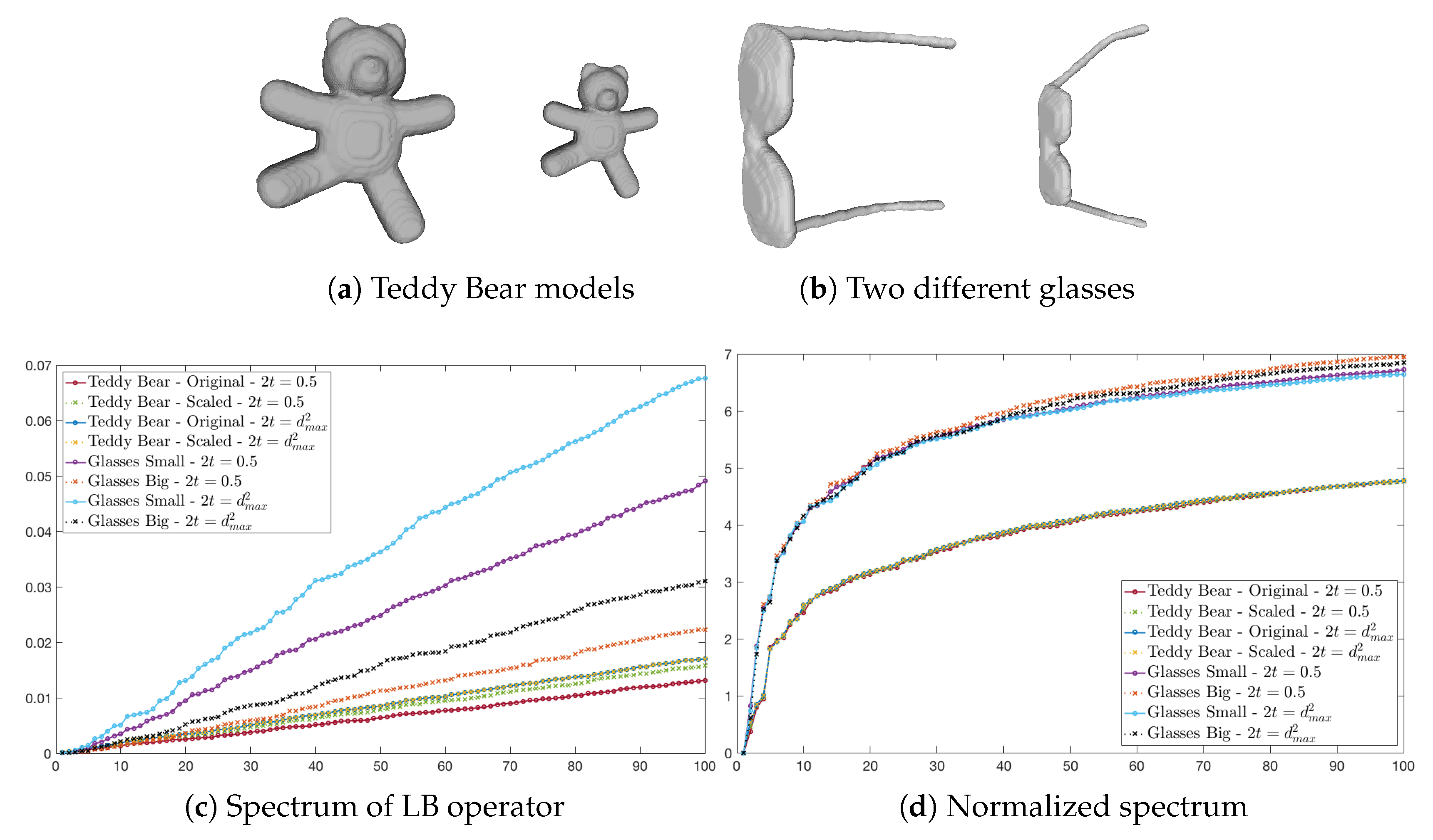
3.2. Scale Normalization

For some applications, the size of an object is not a determinant factor in shape comparison and identification. Therefore, a scale-invariant shape descriptor with a solid normalization method is more desirable. For that purpose, some shape descriptors including Shape-DNA, have proposed multiple normalization methods. Most normalization methods of Shape-DNA focus on finding an appropriate scaling factor, such as the surface area, the volume, or coefficient of a fitting curve, which will be multiplied in the descriptor.
Moreover, it is shown that eigenvalues with a higher order are more susceptible to noise. For that reason, the original Shape-DNA recommends cropping the spectrum and using no more than 100 eigenvalues [20]. In this section, we propose a simple and efficient normalization method that significantly reduces the effect of scale variations as well as noise. In this approach, we are interested in taking the scaling factor out from the descriptor in one step, rather than an extra step to find an appropriate neutralizing factor. Although the normalization seems simple, later in the experiments section, we show its efficiency.
In general, there are two forms of scaling that can affect a shape descriptor: (1) when an arbitrary scale object is scaled in the Euclidean space with factor α , e.g., a Teddy Bear model and its scaled version shown in Figure 2a; and (2) when two objects within a same category are naturally in different sizes, e.g., the two glasses shown in Figure 2b. According to Weyl’s law [48], the eigenvalues of a scaled object (the first form of object scaling) are scaled with factor 1 / α 2 . In the case of the second form of object scaling, the relationship between the eigenvalues of two objects is a complicated relation, which requires solving Equation (10). However, we can approximately model it with f ( α 2 ) —a function of α 2 .
For Equation (6), one can use a constant value for parameter t on the entire dataset, or use a varying value for each object in proportion to the size of the object. For example, as we previously suggested in Equation (7), t can be a multiple of d m a x 2 for each individual object. When t is selected using the latter option, the scaling factor α of the first form of object scaling is canceled out from the numerator and denominator of Equation (6). As a result, all edge weights, and consequently, all eigenvalues will be invariant of the factor α . However, such a parameter t cannot completely deal with the scaling differences between two different objects. In addition, when t is constant for the entire dataset, both forms of object scaling have their impact on the spectrum. Figure 2c shows the spectrum of Teddy Bear models and both glasses in two scenarios; t = 0.5 and t = d m a x 2 . Note that, when t = d m a x 2 , the spectrum of the scaled Teddy Bear model is aligned with the spectrum of the original model.
Another observation from Figure 2c is that the spectrum is a function of t, as well. That phenomenon can be expected as t presents in the exponential term defining edge weights. Let ζ s = g ( α 2 , t ) ( λ 1 , , λ d ) be a LESI descriptor obtained from a scaled 3D model with unknown factor α . To normalize the descriptor and eliminate the effect of the scaling factor as well as parameter t, we recommend computing:
ζ n ( i ) = log ( ζ s ( i ) ) log ( ζ s ( 1 ) ) , for 1 i d
To achieve a scale invariant shape descriptor, we first take the logarithm of the descriptor vector and then compute the difference of the new vector from its smallest element. This is equivalent to dividing the vector by its first element—as suggested by Reuter et al. [20]—and taking the logarithm next. The proposed scale normalization scheme not only normalizes the descriptor to scale variations, but also eliminates the influence of both parameter t and the noise that is present in eigenvalues with a higher order. Basically, division takes the factor out, and the logarithm eliminates the influence of noise. In other words, taking the logarithm of the spectrum takes away g ( α 2 , t ) from multiplicand and leaves it as augend. Then, subtracting one term (e.g., the first element) removes it from all other terms, which is also owed to the monotonicity of the logarithmic function.
As shown in Figure 2d, the normalized spectrum obtained from glasses are nicely grouped together, while they are well-separated from Teddy Bear models, for both cases when t is constant or chosen to be in proportion to the scale of each object.

3.3. Algorithm

Our proposed descriptor consists of three major steps. For a given 3D polygonal model G = ( V , E ) with a set of vertices V = ( x 1 , , x n ) R 3 × n and a set of neighbor connections E, the LESI descriptor is a d-dimensional vector ζ = ( λ 1 , , λ d ) of real and positive values.
In the first step, we compute the n × n real, symmetric, and sparse weight matrix ( W ) for a 1-ring neighbor of every point, as stated in Equation (6) using the inner scaling factor given in Equation (7). Next, we form the generalized eigenvalue problem in Equation (10) by constructing Laplacian and degree matrices ( L and D , respectively) without difficulty. The matrix L is sparse, real, symmetric and semi-positive. Utilizing the Dulmage–Mendelsohn decomposition, we find the number of connected components of L . The objective of the second step is to find the spectrum of the LB operator. For that purpose, we solve the generalized eigenvalue problem using the Lanczos method. Then, we leave out as many smallest eigenvalues as the number of connected components. Since in most cases a single 3D model is made up of one connected component, we only need to leave out one eigenvalue. The last step of the algorithm deals with scale normalization and noise reduction, in the case it is required, by taking the logarithm of the spectrum and subtracting the first element from the rest of the vector. Detailed steps of the algorithm are summarized in Algorithm 1.
Algorithm 1: Laplacian Eigenmap-based scale-invariant global shape descriptor.
Algorithms 12 00171 i001

4. Experiments

In Section 4.1, we first present the two public datasets used in our experiments. Then, in Section 4.2, we qualitatively visualize and measure the competence of the proposed method in discriminating different clusters compared with candidate methods from the literature. Next, in Section 4.3, we validate the effectiveness of the LESI descriptor to distinct multiple classes by measuring the accuracy of multi-class classification. Finally, in Section 4.4, extensive experiments carried out to study the robustness of the proposed shape descriptor with respect to noise, scale invariance, and down-sampling are presented. All experiments were carried out using the MATLAB R2017b environment running on a personal computer with Intel(R) Xeon(R) E3-1245 CPU @ 3.50GHz and 32GB memory.

4.1. Dataset

To validate the utility of the proposed shape descriptor, we utilized two standard, widely-used, and publicly available datasets of 3D polygon meshes. The high-resolution TOSCA dataset [49] contains 80 three-dimensional non-rigid models, including 11 cats, 6 centaurs, 9 dogs, 4 gorillas, 8 horses, 12 women poses, 3 wolves and 2 men with 7 and 20 poses, respectively. In our experiments, we used all models except the gorilla models, as they contain isolated points. The models in each class of the TOSCA dataset are almost identical in terms of scale, the number of vertices, quality of triangulation, and structure, which all represent the same object with different poses.
The McGill dataset with articulating parts [50] was used to evaluate the ability of the descriptors to describe models with poor intra-class quality. The McGill dataset contains 3D models of 30 ants, 30 crabs, 25 glasses, 20 hands, 29 humans, 25 octopuses, 20 pliers, 25 snakes, 31 spiders, and 20 Teddy bears. The classification of the McGill dataset models is more challenging due to scale and shape variations.

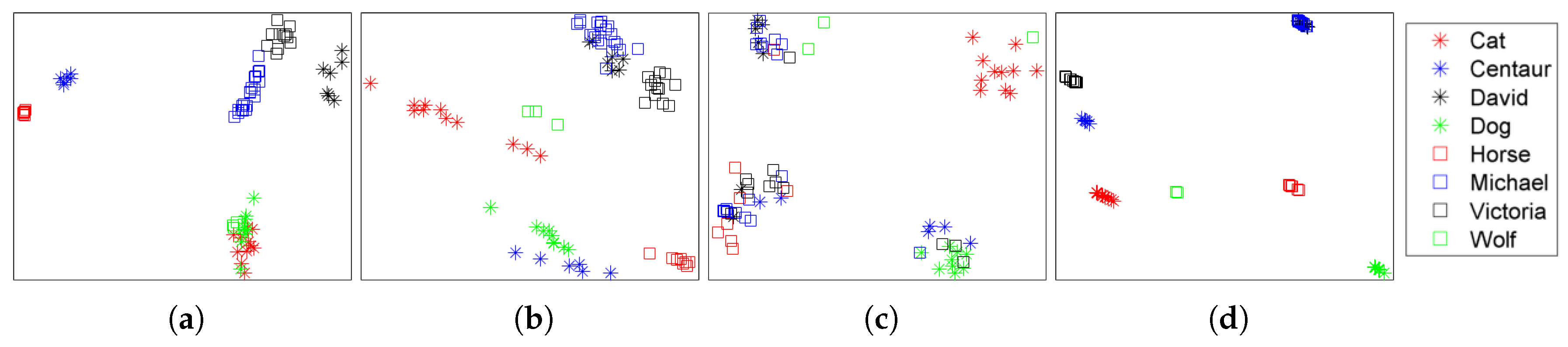
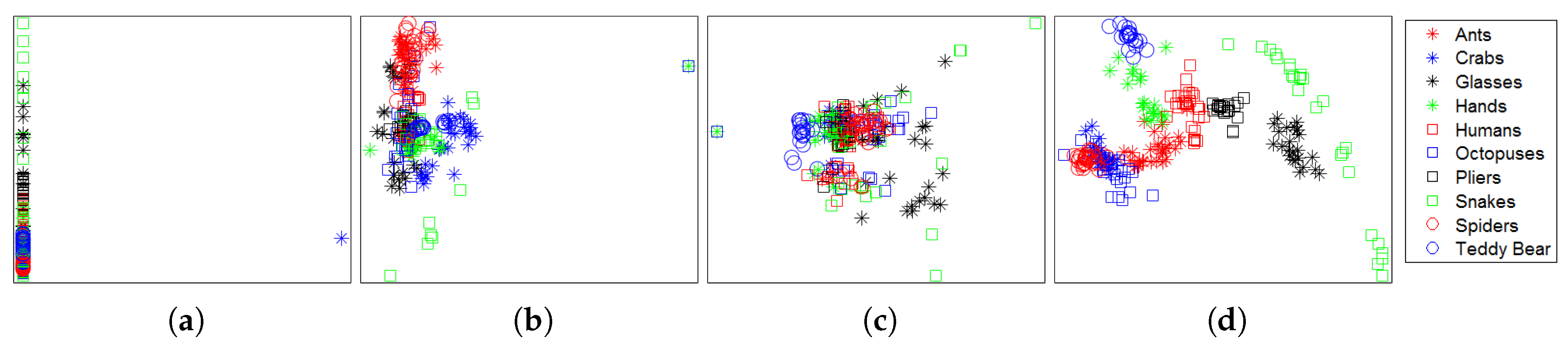
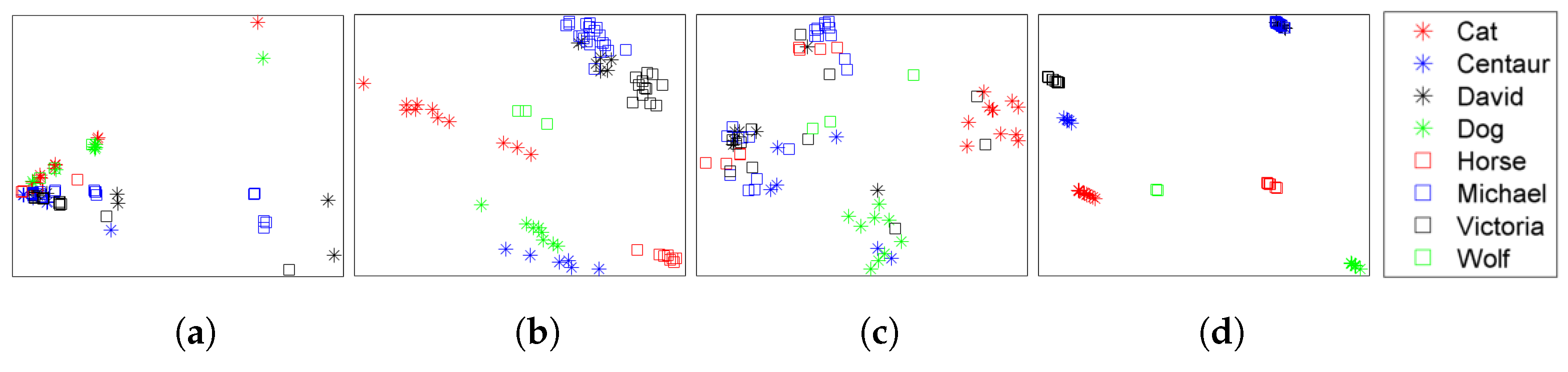
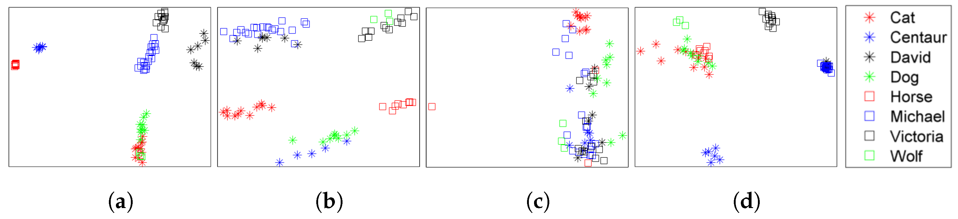
4.2. Retrieval Results

In this section, we evaluate the general performance of our proposed shape descriptor and compare it with several state-of-the-art spectral-based global shape descriptors including Shape-DNA [20], cShape-DNA [30], and GPS [23] algorithms. We chose these methods because they are widely used by researchers (e.g., [51,52,53]) to develop new descriptors or applications, or to evaluate the performance of their proposed descriptors. Moreover, cShape-DNA represents the normalized version of the original Shape-DNA. Even though there are multiple ways to convert a local point descriptor to a global shape fingerprint, in this article we focus only on algorithms that have been originally introduced as global fingerprints. To this end, we take advantage of the source code made available on Dr. Kokkinos’s homepage (http://vision.mas.ecp.fr/Personnel/iasonas/descriptors.html) [28], as well as the shape descriptor package provided by Li et al. [54] available on a GitHub repository (https://github.com/ChunyuanLI/spectral_descriptors) to generate the Shape-DNA and GPS descriptors, respectively. We also compare the performance of shape retrieval using the code provided for evaluation by SHREC’11 [55].
The shape descriptors are compared using the TOSCA dataset to discriminate between different classes of 3D objects. In this experiment, we used the first 33 non-zero eigenvalues ( d = 33 ) . Then, to visualize the locations of objects in the shape space, we projected them onto a 2D plane using Principle Component Analysis (PCA). Figure 3 displays the effectiveness of our method compared with the fingerprints of interest.
Figure 3 reveals that LESI can differentiate models of various classes significantly better than the other methods for a refined and normalized dataset. Despite the large isometric deformations in each class, the proposed LESI method clusters all models of the same class together very tightly. Even though all human models (David, Michael, and Victoria) are very similar, it can distinguish the woman from the men. However, it fails to discriminate models of Michael from David.
Looking more closely at Figure 3 and comparing the performance of Shape-DNA and cShape-DNA in the separation of David and Michael, we conjecture whether objects’ scale is one of the most distinctive features of David and Michael’s differentiation. LESI descriptor is invariant to isometry, object’s location, and rotation. LESI learns the overall structure of each model, which it is similar for men models. We suspect that using the parameter t as defined in Equation (7) may cause LESI to fail to discriminate models of different men. Therefore, we computed LESI descriptor for David and Michael, using t = 5 and t = 15 . Figure 4 shows two samples of David and Michael, which demonstrates how much they look alike. In addition, PCA projection of LESI descriptors for all models of David and Michael using three different values for t—two constant and one variable in proportion to the size of each model—is shown. From the results in Figure 4, we conclude that LESI algorithm can differentiate different models of men, if we use constant t value. However, for the sake of simplicity and consistency, we continue the rest of this section using t as defined in Equation (7).
To demonstrate the power of our method in classifying objects with low intra-class similarity compared with other shape descriptors, the same experiment was carried out on the McGill dataset. Models of the same class with articulating parts are in different scales, shape, and structure. The 2D PCA projections of 33-dimension descriptors from all four algorithms are shown in Figure 5.
As illustrated in Figure 5, the original Shape-DNA is highly sensitive to scales. Multiple methods are presented in [20] to make the descriptor normalized to scale. cShape-DNA represents a normalized version of it by multiplying the descriptor with the surface area. Although cShape-DNA can separate models from each other, classes are not separated efficiently. LESI outperforms the other algorithms by providing distinct descriptors, which can separate classes. Shape descriptors offered by LESI prove superior to the other algorithms in the shape retrieval and classification tasks, as described below and in the next section, respectively.
To examine the superiority of LESI quantitatively, we computed multiple standard retrieval measures including Nearest Neighbor (NN), First Tier (FT), Second Tier (ST), e-Measure (E), and Discounted Cumulative Gain (DCG). These measures represent state-of-the-art quality metrics used when evaluating matching results for shape-based search engines [56]. Table 1 reports the results of shape retrieval. Boldface numbers indicate the highest value for each measure per each dataset. In Table 1, it is clear that the LESI descriptor outperforms all other methods concerning all measures in retrieving models from the McGill dataset. When retrieving models of the TOSCA dataset, LESI outperforms all methods concerning FT, ST, and E measures. Shape-DNA outperforms LESI by a higher value for NN and DCG measures, due to the poor discrimination between David and Michael performed by the LESI descriptor. However, it does not diminish the validity of our claim that LESI performs well for meshes with non-uniform sampling or peculiarities.

4.3. Multi-Class Classification Results
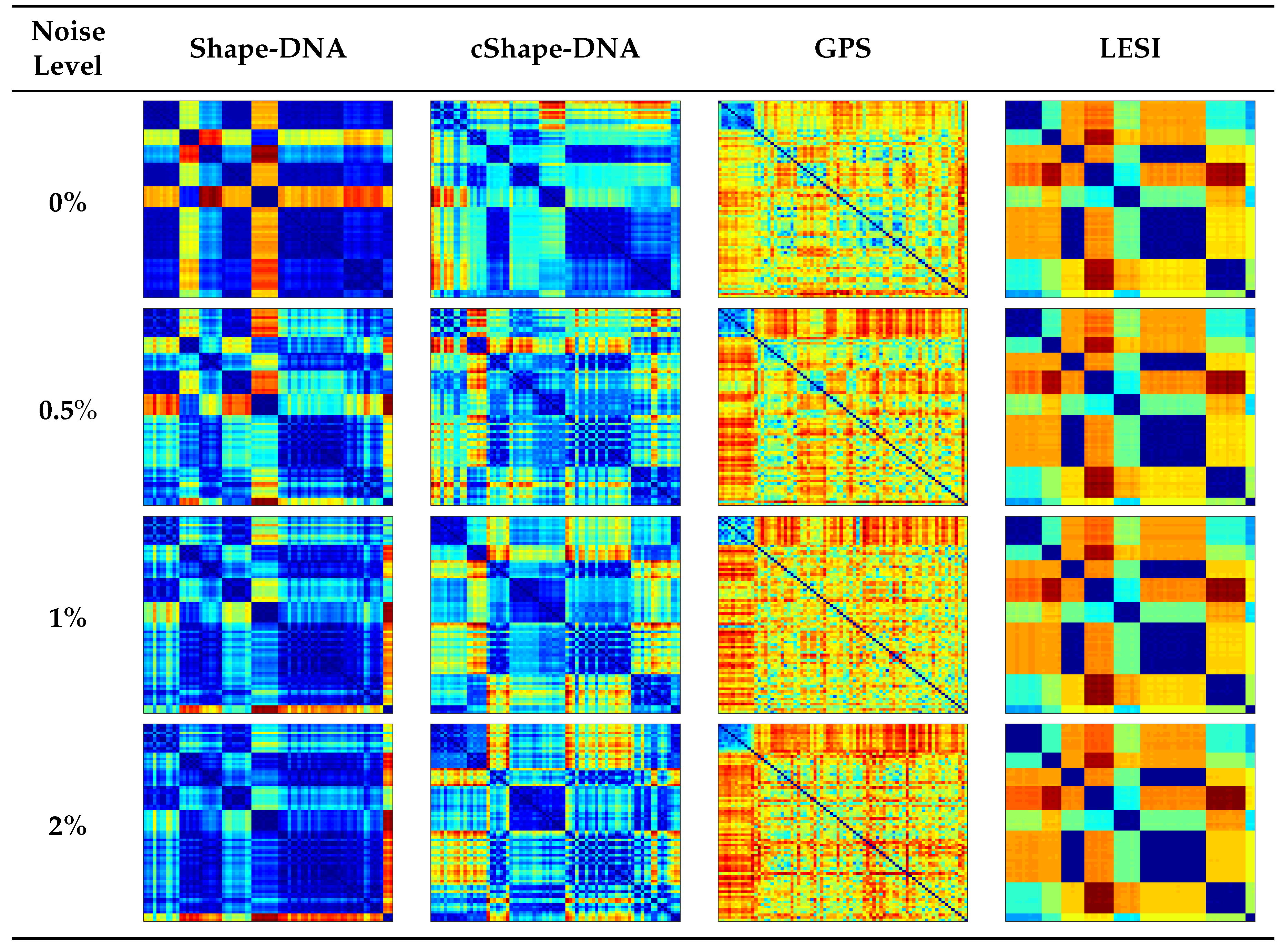
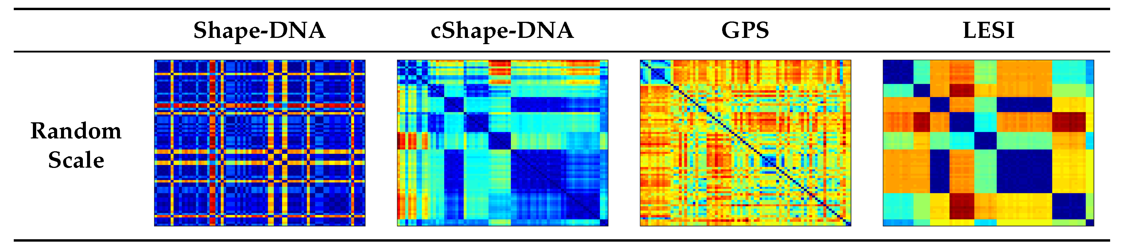
In this section, we corroborate the findings of Section 4.2 by training a linear multi-class SVM classifier to assess the accuracy of LESI compared to other shape descriptors. For this experiment, we utilized the McGill dataset. In addition to the shape descriptors evaluated in Section 4.2, we computed another normalized version of Shape-DNA by dividing the feature vector by its first element (similar to what LESI offers) as suggested in [20]. This way we can compare the effect of the exponential weighting scheme without the influence of the normalization method or compactness (offered by cShape-DNA). Using 10-fold cross-validation and repeating the experiment three times, we report the average accuracy for each method in Table 2.
The new LESI approach significantly outperforms all other methods when using a two-tailed paired t-test ( p < 0.05 ) . The t-test was performed on one set of 10 folds in order to avoid violating the independence assumption of the t-test. There is a significant improvement in accuracy when comparing the Shape-DNA (Normalized) to other variants of the Shape-DNA, which is due in part to the normalization method. However, the average accuracy of the LESI descriptor is noticeably higher (95%) when compared to 90% of the Shape-DNA (Normalized).
Finally, Figure 6 shows the confusion matrix obtained from the linear multi-class SVM using LESI descriptor. The number of correct classifications made for each class (indicated by the green diagonal), confirms that our method captures the discriminative features of the shapes.

4.4. Robustness

In this section, we address the robustness of the LESI shape descriptor to shape variations, including noise, scale, and down-sampling by performing another set of experiments. First, we generated the disturbed version of every model in the TOSCA dataset. Then, we tested the capability of every method mentioned above in discriminating between different classes. For this purpose, besides plotting the 2D PCA projection of shape descriptors, we also computed and plotted the pairwise Euclidean distance matrix, in every case. The distance matrix represents the dissimilarity between each pair of models in the set. It is often used to compute other evaluating metrics such as nearest-neighbor, and first and second tier, to name a few. The dissimilarity of descriptors increases from blue to red, and the more separate classes differ in color, the better they are discriminating from each other.
Resistance to noise. Multiple noisy versions of the TOSCA dataset were generated following the idea articulated in [57]. To this end, the surface meshes of all models were disturbed by changing the position of each point along its normal vector that was chosen randomly from an interval ( L , L ) with the 0 mean, where L determines the noise level and is a fraction of the diagonal length of the model bounding box. In this experiment, three noise levels L = 0.5 % , L = 1 % , and L = 2 % were tested, where the latter one represents a greater level of noise. Two-dimensional PCA projections of all descriptors with the presence of different levels of noise are plotted in Figure 7. Combining these with the results shown in Figure 3, where no noise is present, demonstrates that the LESI algorithm is highly noise-resistant while the performance of the Shape-DNA and cShape-DNA decreases as the level of noise increases. Moreover, GPS fails in separating different classes of models with the presence of noise. Figure 8 reflects the effect of noise on the discriminative power of the descriptors. The LESI algorithm shows consistent results as the level of noise increases from 0% (top row) to 2% (bottom row).
Scale invariance. To validate the insensitivity of the LESI descriptor to scale variations and compare the robustness of the proposed method with other descriptors, each model of the TOSCA dataset was scaled by a factor of 0.5, 0.875, 1.25, 1.625, or 2 randomly. Figure 9 shows that the LESI algorithm surpasses other methods in discerning different classes. Comparing the result of this experiment with the results shown in Figure 3 demonstrates the consistency of the LESI and cShape-DNA algorithms with the presence of scale variation. That is expected, as they can remove the parameter of scale and obtain scale-free descriptors. The distance matrices in Figure 10 show that the original Shape-DNA algorithm is very susceptible to scale variations. Even though the cShape-DNA has significantly improved scale sensitivity of the original Shape-DNA, it does not provide as accurate results as the LESI algorithm does.
Resistance to the sampling rate. To investigate the effect of sampling rates on the discriminative power of the shape descriptors, Bronstein et al. [8] proposed to reduce the number of vertices to 20% of its original size. Accordingly, the down-sampled version of the TOSCA dataset was generated, and shape descriptors associated with them were computed. The 2D PCA projections and distance matrices of descriptors are illustrated in Figure 11 and Figure 12, respectively. Although the original Shape-DNA shows a more accurate result than cShape-DNA, the separation of cat, dog, and wolf models is challenging. Although the performance of the LESI method is slightly affected, it still outperforms cShape-DNA and GPS methods.

5. Discussion

In this study, motivated by the unique properties of Laplacian Eigenmap (i.e., locality preservation, structural equivalence, and dimensionality reduction) and inspired by the existing spectral-based shape descriptors, we investigated the application of manifold learning in deriving a shape fingerprint in order to address the limitations tied to popular cotangent-based shape descriptors. We proposed a global descriptor (LESI) with an easy-to-compute and efficient normalization technique that facilitates applications such as shape classification and retrieval. Our method applies fewer restrictions on the class of meshes as well as improves the quality of tessellations. Analogous to other spectral descriptors, LESI uses the spectrum of the LB operator, which is independent of the shape location, informative (contains a considerable amount of geometrical and topological information), and above all isometric invariant. We compared the discriminating power of LESI with three prominent descriptors from the literature, namely Shape-DNA, cShape-DNA, and GPS, and found it to be superior.
In the first set of experiments illustrated in Figure 3 and Figure 5, our method substantially outperforms the others. The superiority of LESI is more significant when the McGill dataset is used (Table 2 and Figure 6). This dataset includes wide variations in mesh structure and scales, causing the failure of the other methods to generate acceptable results. However, LESI, due to utilizing a different method of discretization to form the LB operator, focuses on the vicinity rather than the quality of the triangulation. Therefore, our technique, unlike other methods, is not affected by the low quality of polygon meshes.
The second set of experiments evaluated the reliability of our method in the presence of noise, scale variations, as well as different sampling rates. LESI shows impressive robustness against the first two sets of perturbation. Despite the negative impact of down sampling in LESI descriptor, it continues to show better performance when compared to cShape-DNA and GPS. It should be noted that the result could also be improved by increasing the size of the output vector.
In addition to the discriminating power of the descriptor, degenerate and non-uniform meshes may also cause failure of an algorithm to converge. The cotangent weight-based algorithms were not able to compute the descriptors for two shapes from the McGill dataset. GPS also failed to compute descriptors for six models of the down sampled TOSCA dataset. However, our technique converges at all times despite the quality of the polygon mesh structure.
Moreover, LESI, unlike cotangent weight-based techniques, is not confined to the triangulated meshes as it disregards the mesh geometry [58]. LESI inherits this property from the capability of manifold learning techniques in coping with high dimensional data. The discretization of the LB operator using cotangent weights on the quadrilateral meshes is not as straightforward as on triangular meshes. To compute the LB operator on a quadrilateral mesh, all rectangles need to be divided into triangles. It could be done easily; however, as for each quad there are two possible triangulations, thus the result is not unique.
The time needed to compute a descriptor, for all spectral-based descriptors discussed in this research, can be divided into two parts: (1) constructing the L and D matrices; and (2) solving the generalized eigenvalue problem. The computation time depends on n (graph size) and d (descriptor length). The computation cost increases quadratically with n as does the size of matrices. Running the experiments on a desktop with system specifications mentioned on Section 4, the average total time is 1.18 and 2.29 s with Shape-DNA and LESI algorithms as well as 0.41 and 0.90 s with Shape-DNA and LESI algorithms using TOSCA and McGill datasets, respectively. However, the Shape-DNA code for computing the first part is accelerated by using C MEX files, which makes it incomparable with our method. Therefore, we timed solving the generalized eigenvalue problem, reported as follows: on average it takes 1 and 0.97 s with Shape-DNA and LESI algorithms using TOSCA dataset (p-value = 0.64, not statistically significant), as well as 0.35 and 0.40 s with Shape-DNA and LESI algorithms using McGill dataset (p-value < 0.05, statistically significant). We compared our method with Shape-DNA as it is the basis of cotangent-based descriptors. Other cotangent-based methods have one or more extra steps, which add fraction of seconds. The time difference between these methods are negligible when descriptors are computed using a system with enough RAM, which is easily accessible in today’s world. Therefore, with respect to the computational cost, neither of these methods has advantage over the other.
In the original Laplacian Eigenmaps, the high dimension data require a considerable amount of processing as the list of all connections need to be computed for the dataset. In fact, for each point in the high dimension space, a given number of nearest neighbors need to be extracted which could be challenging and unmanageable. However, applying this technique to the 3D meshes, we skip this step as the neighbors are already defined and given in the mesh structure.
This work benefits from the Laplacian Eigenmap technique in a space in which the vicinities are given. LESI takes advantage of simple Laplacian computation, to form the LB operator, which provides concise and informative shape descriptors. Experimental results prove that LESI is more effective compared with the other powerful descriptors.
One limitation of LESI is related to the original Laplacian Eigenmap algorithm introduced by Belkin and Niyogi, in which the generalized eigenvalue problem was solved without specifying a boundary condition. It is not clear how the algorithm can handle manifolds with boundaries. Therefore, we limited our experiments to 3D shapes with closed manifolds. Not necessarily a limitation, but a matter of concern, is how the algorithm works in differentiating different models of men (David and Michael). While parameter t provides one degree of freedom for the algorithm, it is data-dependent and needs to be assigned carefully using cross-validation or the validation set approach. It accepts a wide range of values and no unique value is required.
Although we investigated only the application of Laplacian Eigenmap in introducing a shape descriptor, there are some other spectral-based manifold learning methods, such as Isomap, LLE, and Diffusion map, which have not been examined. Another possible future work can be investigating the possibility of extending the current contribution to other data modalities, e.g., classification of 2D images/sketches. One can construct a graph from a single 2D image by extracting features from all or sampled pixels. Such an approach benefits from the fact that there is no limit to the number of extracted features when using Laplacian Eigenmap.
In the end, even though the focus of this research has been on spectral shape descriptors, we would like to briefly discuss where our method can stand in comparison with learning-based methods. Recently, we have witnessed that deep learning methods have superseded traditional methods in many applications. Several deep learning techniques, (e.g., [59,60,61]) have been introduced in this area. The process of training a neural network is very time consuming and requires high performance computing units, i.e., a GPU. However, they are capable of learning great deal of structural variations among objects within the same category. To achieve the goal of learning by seeing, they require a large and well-annotated sample set. In some applications, such as medical image analysis, obtaining a dataset with characteristics mentioned above is very challenging. In those cases, deep learning techniques may result in over-fitting. One approach to mitigate this issue is integrating independent feature sets, e.g., spectra of LB operator, with features extracted by learning methods. Recent research has shown that, in the case of small datasets, while spectral and deep-based methods may demonstrate similar behavior in terms of accuracy, their combination improves the total accuracy. In addition, as they can be computed in parallel, they do not constrain runtime execution. This brief comparison requires more investigation both experimentally and theoretically.

6. Conclusions

With recent advances in imaging and data processing, shape analyses have found applications in various fields, from archaeology to bio-informatics. The current contribution utilizes Laplacian Eigenmap as a foundation, and introduces a simple, easy-to-implement, yet efficient global shape fingerprint. We have shown that the spectrum of LB operator that is discretized using exponential weighting scheme can efficiently represent a 3D shape, which can be used for object retrieval and classification. We have equipped our descriptor with an optional, straight-forward normalization method, which makes it suitable for applications in which scale-invariant and noise-resistant descriptors are preferred. The proposed shape fingerprint belongs to the category of spectral shape descriptors, which does not require training, as deep-learning based methods do. The proposed descriptor, as well as being used alone in geometry analysis problems, can be combined with learning-based methods to improve their performance. For example, in problems in which the number of samples is not enough, adding features extracted independently by a spectral method can prevent learning methods from over-fitting. Two possible extensions to our work could be investigating the applicability of the proposed descriptor in differentiating 3D objects with boundaries (e.g., 3D planes), and utilizing computed eigenvectors for graph partitioning. In the end, we conclude that manifold learning methods can be used to develop new spectral-based shape descriptors to learn the structure of manifolds despite the quality of sampled meshes.

Author Contributions

Conceptualization, F.S.B. and R.R.; methodology, F.S.B. and R.R.; software, F.S.B. and R.R.; formal analysis, F.S.B.; writing—original draft preparation, F.S.B. and R.R.; writing—review and editing, F.S.B., R.R., P.P., R.M.D. and Z.Y.; and visualization, F.S.B.

Funding

This research received financial support from GE Healthcare through the UWM Catalyst Grant program, the Center for Predictive Computational Phenotyping supported by the National Institutes of Health Big Data to Knowledge (BD2K) Initiative under Award Number U54 AI117924, and the grant UL1TR002373 from the Clinical and Translational Science Award (CTSA) program of the National Center for Advancing Translational Sciences, NIH.

Acknowledgments

Our sincere thanks goes to Ahmad P. Tafti and C. David Page for their expertise and constructive comments. Any errors are our own and should not tarnish the reputation of these esteemed scientists.

Conflicts of Interest

The authors declare no conflict of interest.

References

  1. Omrani, E.; Tafti, A.P.; Fathi, M.F.; Moghadam, A.D.; Rohatgi, P.; D’Souza, R.M.; Yu, Z. Tribological study in microscale using 3D SEM surface reconstruction. Tribol. Int. 2016, 103, 309–315. [Google Scholar] [CrossRef]
  2. Ng, L.; Pathak, S.; Kuan, C.; Lau, C.; Dong, H.W.; Sodt, A.; Dang, C.; Avants, B.; Yushkevich, P.; Gee, J.; et al. Neuroinformatics for genome-wide 3-D gene expression mapping in the mouse brain. IEEE/ACM Trans. Comput. Biol. Bioinf. (TCBB) 2007, 4, 382–393. [Google Scholar] [CrossRef] [PubMed]
  3. Gao, Z.; Rostami, R.; Pang, X.; Fu, Z.; Yu, Z. Mesh generation and flexible shape comparisons for bio-molecules. Mol. Based Math. Biol. 2016, 4, 1–13. [Google Scholar] [CrossRef]
  4. Sosa, G.D.; Rodríguez, S.; Guaje, J.; Victorino, J.; Mejía, M.; Fuentes, L.S.; Ramírez, A.; Franco, H. 3D surface reconstruction of entomological specimens from uniform multi-view image datasets. In Proceedings of the 2016 XXI Symposium on Signal Processing, Images and Artificial Vision (STSIVA), Bucaramanga, Colombia, 31 August–2 September 2016; pp. 1–8. [Google Scholar] [CrossRef]
  5. Riehemann, S.; Palme, M.; Kuehmstedt, P.; Grossmann, C.; Notni, G.; Hintersehr, J. Microdisplay-based intraoral 3D scanner for dentistry. J. Disp. Technol. 2011, 7, 151–155. [Google Scholar] [CrossRef]
  6. Wu, C.; Bradley, D.; Garrido, P.; Zollhöfer, M.; Theobalt, C.; Gross, M.; Beeler, T. Model-based teeth reconstruction. ACM Trans. Graph. (TOG) 2016, 35, 220. [Google Scholar] [CrossRef]
  7. Aflalo, Y.; Bronstein, A.M.; Bronstein, M.M.; Kimmel, R. Deformable shape retrieval by learning diffusion kernels. In International Conference on Scale Space and Variational Methods in Computer Vision; Springer: Berlin, Germany, 2011; pp. 689–700. [Google Scholar]
  8. Bronstein, A.M.; Bronstein, M.M.; Guibas, L.J.; Ovsjanikov, M. Shape google: Geometric words and expressions for invariant shape retrieval. ACM Trans. Graph. (TOG) 2011, 30, 1. [Google Scholar] [CrossRef]
  9. Xie, J.; Fang, Y.; Zhu, F.; Wong, E. Deepshape: Deep learned shape descriptor for 3d shape matching and retrieval. In Proceedings of the IEEE Conference on Computer Vision and Pattern Recognition, Boston, MA, USA, 7 June 2015; pp. 1275–1283. [Google Scholar]
  10. Toldo, R.; Castellani, U.; Fusiello, A. Visual vocabulary signature for 3D object retrieval and partial matching. In Proceedings of the 2nd Eurographics conference on 3D Object Retrieval; Eurographics Association: Aire-la-Ville, Switzerland, 2009; pp. 21–28. [Google Scholar]
  11. Bu, S.; Liu, Z.; Han, J.; Wu, J.; Ji, R. Learning high-level feature by deep belief networks for 3-D model retrieval and recognition. IEEE Trans. Multimed. 2014, 16, 2154–2167. [Google Scholar] [CrossRef]
  12. Boscaini, D.; Masci, J.; Rodolà, E.; Bronstein, M.M.; Cremers, D. Anisotropic diffusion descriptors. Comput. Graph. Forum 2016, 35, 431–441. [Google Scholar] [CrossRef]
  13. Bronstein, A.M. Spectral descriptors for deformable shapes. arXiv 2011, arXiv:1110.5015. [Google Scholar]
  14. Raviv, D.; Kimmel, R.; Bruckstein, A.M. Graph isomorphisms and automorphisms via spectral signatures. IEEE Trans. Pattern Anal. Mach. Intell. 2013, 35, 1985–1993. [Google Scholar] [CrossRef]
  15. De Youngster, D.; Paquet, E.; Viktor, H.; Petriu, E. An isometry-invariant spectral approach for protein-protein docking. In Proceedings of the 13th IEEE International Conference on BioInformatics and BioEngineering, Chania, Greece, 10–13 December 2013; pp. 1–6. [Google Scholar]
  16. Ovsjanikov, M.; Ben-Chen, M.; Solomon, J.; Butscher, A.; Guibas, L. Functional maps: A flexible representation of maps between shapes. ACM Trans. Graph. (TOG) 2012, 31, 30. [Google Scholar] [CrossRef]
  17. Tangelder, J.W.; Veltkamp, R.C. A survey of content based 3D shape retrieval methods. In Proceedings of the 2004 Shape Modeling Applications, Genova, Italy, 7–9 June 2004; pp. 145–156. [Google Scholar]
  18. Zhang, L.; da Fonseca, M.J.; Ferreira, A.; e Recuperação, C.R.A. Survey on 3D Shape Descriptors; Technical Report, DecorAR (FCT POSC/EIA/59938/2004); Fundação para a Cincia e a Tecnologia: Lisboa, Portugal, 2007. [Google Scholar]
  19. Rostami, R.; Bashiri, F.; Rostami, B.; Yu, Z. A survey on data-driven 3D shape descriptors. Comput. Graph. Forum 2019, 38, 356–393. [Google Scholar] [CrossRef]
  20. Reuter, M.; Wolter, F.E.; Peinecke, N. Laplace–Beltrami spectra as ’Shape-DNA’ of surfaces and solids. Comput. Aided Des. 2006, 38, 342–366. [Google Scholar] [CrossRef]
  21. Sun, J.; Ovsjanikov, M.; Guibas, L. A concise and provably informative multi-scale signature based on heat diffusion. Comput. Graph. Forum 2009, 28, 1383–1392. [Google Scholar] [CrossRef]
  22. Aubry, M.; Schlickewei, U.; Cremers, D. The wave kernel signature: A quantum mechanical approach to shape analysis. In Proceedings of the IEEE 2011 Conference on Computer Vision Workshops (ICCV Workshops), Barcelona, Spain, 6–13 November 2011; pp. 1626–1633. [Google Scholar]
  23. Rustamov, R.M. Laplace-Beltrami eigenfunctions for deformation invariant shape representation. In Proceedings of the Fifth Eurographics Symposium on Geometry Processing; Eurographics Association: Aire-la-Ville, Switzerland, 2007; pp. 225–233. [Google Scholar]
  24. Reuter, M.; Biasotti, S.; Giorgi, D.; Patanè, G.; Spagnuolo, M. Discrete Laplace–Beltrami operators for shape analysis and segmentation. Comput. Graph. 2009, 33, 381–390. [Google Scholar] [CrossRef]
  25. Belkin, M.; Sun, J.; Wang, Y. Discrete laplace operator on meshed surfaces. In Proceedings of the ACM Twenty-Fourth Annual Symposium on Computational Geometry, College Park, MD, USA, 9–11 June 2008; pp. 278–287. [Google Scholar]
  26. Goldberg, Y.; Zakai, A.; Kushnir, D.; Ritov, Y. Manifold learning: The price of normalization. J. Mach. Learn. Res. 2008, 9, 1909–1939. [Google Scholar]
  27. Belkin, M.; Niyogi, P. Laplacian eigenmaps for dimensionality reduction and data representation. Neural Comput. 2003, 15, 1373–1396. [Google Scholar] [CrossRef]
  28. Bronstein, M.M.; Kokkinos, I. Scale-invariant heat kernel signatures for non-rigid shape recognition. In Proceedings of the 2010 IEEE Computer Society Conference on Computer Vision and Pattern Recognition, San Francisco, CA, USA, 13–18 June 2010; pp. 1704–1711. [Google Scholar]
  29. Kuang, Z.; Li, Z.; Lv, Q.; Weiwei, T.; Liu, Y. Modal function transformation for isometric 3D shape representation. Comput. Graph. 2015, 46, 209–220. [Google Scholar] [CrossRef]
  30. Gao, Z.; Yu, Z.; Pang, X. A compact shape descriptor for triangular surface meshes. Comput. Aided Des. 2014, 53, 62–69. [Google Scholar] [CrossRef] [PubMed] [Green Version]
  31. Lévy, B. Laplace-beltrami eigenfunctions towards an algorithm that “understands” geometry. In Proceedings of the IEEE International Conference on Shape Modeling and Applications 2006 (SMI’06), Matsushima, Japan, 14–16 June 2006; p. 13. [Google Scholar]
  32. Taubin, G. A signal processing approach to fair surface design. In Proceedings of the ACM 22nd Annual Conference on Computer Graphics and Interactive Techniques, Los Angeles, CA, USA, 6–11 August 1995; pp. 351–358. [Google Scholar]
  33. Mayer, U.F. Numerical solutions for the surface diffusion flow in three space dimensions. Comput. Appl. Math. 2001, 20, 361–379. [Google Scholar]
  34. Xu, G. Discrete Laplace–Beltrami operators and their convergence. Comput. Aided Geom. Des. 2004, 21, 767–784. [Google Scholar] [CrossRef]
  35. Desbrun, M.; Meyer, M.; Schröder, P.; Barr, A.H. Implicit fairing of irregular meshes using diffusion and curvature flow. In Proceedings of the 26th Annual Conference on Computer Graphics and Interactive Techniques; ACM Press/Addison-Wesley Publishing Co.: New York, NY, USA, 1999; pp. 317–324. [Google Scholar] [Green Version]
  36. Meyer, M.; Desbrun, M.; Schröder, P.; Barr, A.H. Discrete differential-geometry operators for triangulated 2-manifolds. In Visualization and Mathematics III; Springer: Berlin, Germany, 2003; pp. 35–57. [Google Scholar]
  37. Xu, G. Convergence analysis of a discretization scheme for Gaussian curvature over triangular surfaces. Comput. Aided Geom. Des. 2006, 23, 193–207. [Google Scholar] [CrossRef]
  38. Tenenbaum, J.B.; De Silva, V.; Langford, J.C. A global geometric framework for nonlinear dimensionality reduction. Science 2000, 290, 2319–2323. [Google Scholar] [CrossRef] [PubMed]
  39. Silva, V.D.; Tenenbaum, J.B. Global versus local methods in nonlinear dimensionality reduction. In Proceedings of the 15th International Conference on Neural Information Processing Systems (NIPS’02), Vancouver, BC, Canada, 9–14 December 2002; pp. 721–728. [Google Scholar]
  40. Roweis, S.T.; Saul, L.K. Nonlinear dimensionality reduction by locally linear embedding. Science 2000, 290, 2323–2326. [Google Scholar] [CrossRef] [PubMed]
  41. Saul, L.K.; Roweis, S.T. Think globally, fit locally: Unsupervised learning of low dimensional manifolds. J. Mach. Learn. Res. 2003, 4, 119–155. [Google Scholar]
  42. Coifman, R.R.; Lafon, S. Diffusion maps. Appl. Comput. Harmonic Anal. 2006, 21, 5–30. [Google Scholar] [CrossRef] [Green Version]
  43. Belkin, M.; Niyogi, P. Laplacian eigenmaps and spectral techniques for embedding and clustering. In Proceedings of the 14th International Conference on Neural Information Processing Systems (NIPS’01), Vancouver, BC, Canada, 3–8 December 2001; pp. 585–591. [Google Scholar]
  44. Wachinger, C.; Navab, N. Manifold Learning for Multi-Modal Image Registration. In Proceedings of the British Machine Vision Conference (BMVC’10), Aberystwyth, UK, 30 August–2 September 2010; pp. 82.1–82.12. [Google Scholar]
  45. Wachinger, C.; Navab, N. Structural image representation for image registration. In Proceedings of the 2010 IEEE Computer Society Conference on Computer Vision and Pattern Recognition—Workshops, San Francisco, CA, USA, 13–18 November 2010; pp. 23–30. [Google Scholar]
  46. Shi, J.; Malik, J. Normalized cuts and image segmentation. IEEE Trans. Pattern Anal. Mach. Intell. 2000, 22, 888–905. [Google Scholar] [CrossRef]
  47. Dulmage, A.L.; Mendelsohn, N.S. Coverings of bipartite graphs. Can. J. Math. 1958, 10, 516–534. [Google Scholar] [CrossRef]
  48. Weyl, H. Über die asymptotische Verteilung der Eigenwerte. Nachrichten Gesellschaft Wissenschaften Göttingen Mathematisch-Physikalische Klasse 1911, 1911, 110–117. [Google Scholar]
  49. Bronstein, A.M.; Bronstein, M.M.; Kimmel, R. Numerical Geometry of Non-Rigid Shapes; Springer Science & Business Media: Berlin, Germany, 2008. [Google Scholar]
  50. Siddiqi, K.; Zhang, J.; Macrini, D.; Shokoufandeh, A.; Bouix, S.; Dickinson, S. Retrieving articulated 3-D models using medial surfaces. Mach. Vis. Appl. 2008, 19, 261–275. [Google Scholar] [CrossRef]
  51. Mirloo, M.; Ebrahimnezhad, H. Non-rigid 3D object retrieval using directional graph representation of wave kernel signature. Multimed. Tools Appl. 2017, 77, 6987–7011. [Google Scholar] [CrossRef]
  52. Masoumi, M.; Hamza, A.B. Global spectral graph wavelet signature for surface analysis of carpal bones. arXiv 2017, arXiv:1709.02782. [Google Scholar] [CrossRef] [PubMed]
  53. Boscaini, D.; Masci, J.; Melzi, S.; Bronstein, M.M.; Castellani, U.; Vandergheynst, P. Learning class-specific descriptors for deformable shapes using localized spectral convolutional networks. Comput. Graph. Forum 2015, 34, 13–23. [Google Scholar] [CrossRef]
  54. Li, C.; Hamza, A.B. Spatially aggregating spectral descriptors for nonrigid 3D shape retrieval: a comparative survey. Multimed. Syst. 2014, 20, 253–281. [Google Scholar] [CrossRef]
  55. Lian, Z.; Godil, A.; Bustos, B.; Daoudi, M.; Hermans, J.; Kawamura, S.; Kurita, Y.; Lavoua, G.; Dp Suetens, P. SHREC’11 track: Shape retrieval on non-rigid 3D watertight meshes. In Proceedings of the Eurographics Workshop on 3D Object Retrieval (3DOR), Llandudno, UK, 10 April 2011; pp. 79–88. [Google Scholar]
  56. Shilane, P.; Min, P.; Kazhdan, M.; Funkhouser, T. The princeton shape benchmark. In Proceedings of the International Conference on Shape Modeling and Applications (SMI’04), Genova, Italy, 7–9 June 2004; pp. 167–178. [Google Scholar]
  57. Liu, Y.J.; Chen, Z.; Tang, K. Construction of iso-contours, bisectors, and Voronoi diagrams on triangulated surfaces. IEEE Trans. Pattern Anal. Mach. Intell. 2011, 33, 1502–1517. [Google Scholar] [PubMed]
  58. Zhang, Y.; Bajaj, C.; Xu, G. Surface smoothing and quality improvement of quadrilateral/hexahedral meshes with geometric flow. Int. J. Numer. Methods Biomed. Eng. 2009, 25, 1–18. [Google Scholar] [CrossRef] [PubMed]
  59. Fang, Y.; Xie, J.; Dai, G.; Wang, M.; Zhu, F.; Xu, T.; Wong, E. 3D deep shape descriptor. In Proceedings of the IEEE Conference on Computer Vision and Pattern Recognition (CVPR), Boston, MA, USA, 7–12 June 2015; pp. 2319–2328. [Google Scholar]
  60. Wu, Z.; Song, S.; Khosla, A.; Yu, F.; Zhang, L.; Tang, X.; Xiao, J. 3d shapenets: A deep representation for volumetric shapes. In Proceedings of the IEEE Conference on Computer Vision and Pattern Recognition (CVPR), Boston, MA, USA, 7–12 June 2015; pp. 1912–1920. [Google Scholar]
  61. Qi, C.R.; Su, H.; Mo, K.; Guibas, L.J. PointNet: Deep learning on point sets for 3D classification and segmentation. In Proceedings of the IEEE Conference on Computer Vision and Pattern Recognition (CVPR), Honolulu, HI, USA, 21–26 July 2017; pp. 77–85. [Google Scholar]
Figure 1. The block diagram of the proposed Laplacian Eigenmaps based scale-invariant (LESI) global shape descriptor.
Algorithms 12 00171 g001
Figure 2. An example showing the proposed normalization method of the shape descriptor. (a) A Teddy Bear model and its scaled version (scale factor 0.7). (b) Two different glasses that vary in size. (c) The spectrum of the original Teddy Bear, scaled Teddy Bear, and both glasses with t = 0.5 and t = d m a x 2 . Please note that the spectrum of the original and scaled Teddy Bear models coincide when t = d m a x 2 . (d) The spectrum of all models after proposed normalization.
Algorithms 12 00171 g002
Figure 3. 2D PCA projection of shape descriptors computed from: (a) original Shape-DNA; (b) cShape-DNA; (c) GPS; and (d) LESI algorithms on TOSCA dataset.
Algorithms 12 00171 g003
Figure 4. Experiment on separating different models of men: (a) a sample of Michael (left) and David (right) models; and (b) PCA projection of LESI descriptors of different men models using t = 2 d m a x 2 , t = 5 , and t = 15 .
Algorithms 12 00171 g004
Figure 5. 2D PCA projection of shape descriptors computed from: (a) original Shape-DNA; (b) cShape-DNA; (c) GPS; and (d) LESI algorithms on McGill dataset.
Algorithms 12 00171 g005
Figure 6. Confusion matrix obtained from linear multi-class SVM for McGill dataset using LESI descriptors.
Algorithms 12 00171 g006
Figure 7. 2D PCA projection of shape descriptors computed by (from left to right) Shape-DNA, cShape-DNA, GPS, and LESI algorithms from perturbed TOSCA dataset with (from top to bottom) 0.5%, 1%, and 2% noise level, respectively.
Algorithms 12 00171 g007
Figure 8. The Euclidean pairwise distance matrix of shape descriptors computed by (from left to right) Shape-DNA, cShape-DNA, GPS, and LESI algorithms from perturbed TOSCA dataset by (from top to bottom) 0%, 0.5%, 1%, 2% noise levels.
Algorithms 12 00171 g008
Figure 9. 2D PCA projection of shape descriptors computed by: (a) original Shape-DNA; (b) cShape-DNA; (c) GPS; and (d) LESI algorithms over scaled version of the TOSCA dataset by a randomly chosen factor of 0.5, 0.875, 1.25, 1.625, or 2.
Algorithms 12 00171 g009
Figure 10. The Euclidean pairwise distance matrix of shape descriptors computed by (from left to right) Shape-DNA, cShape-DNA, GPS, and LESI algorithms over scaled version of the TOSCA dataset by a randomly chosen factor of 0.5, 0.875, 1.25, 1.625, or 2.
Algorithms 12 00171 g010
Figure 11. 2D PCA projection of shape descriptors computed by: (a) original Shape-DNA; (b) cShape-DNA; (c) GPS; and (d) LESI algorithms from down sampled TOSCA dataset by rate of 20%.
Algorithms 12 00171 g011
Figure 12. The Euclidean pairwise distance matrix of shape descriptors computed by (from left to right) Shape-DNA, cShape-DNA, GPS, and LESI algorithms from from down sampled TOSCA dataset by rate of 20%.
Algorithms 12 00171 g012
Table 1. Shape retrieval performance using TOSCA and McGill datasets.
DatasetMethodNNFTSTEDCG
TOSCAShapeDNA1.00000.80910.93910.44860.9584
cShapeDNA0.94740.77480.89840.47480.9241
GPS0.48680.42440.63200.36140.6787
LESI0.86840.84560.94300.48600.9244
McGillShapeDNA0.79220.34520.49770.34110.7192
cShapeDNA0.78820.39430.54830.38520.7470
GPS0.38430.25080.40660.25880.6020
LESI0.96470.70460.87390.66440.9251
Table 2. Classification accuracy using McGill dataset.
MethodAverage Accuracy
Shape-DNA21.02%
Shape-DNA (Normalized)90.60%
cShape-DNA71.37%
GPS50.11%
LESI95.69%

