A Study on Sensitive Bands of EEG Data under Different Mental Workloads

Abstract

Electroencephalogram (EEG) signals contain a lot of human body performance information. With the development of the brain–computer interface (BCI) technology, many researchers have used the feature extraction and classification algorithms in various fields to study the feature extraction and classification of EEG signals. In this paper, the sensitive bands of EEG data under different mental workloads are studied. By selecting the characteristics of EEG signals, the bands with the highest sensitivity to mental loads are selected. In this paper, EEG signals are measured in different load flight experiments. First, the EEG signals are preprocessed by independent component analysis (ICA) to remove the interference of electrooculogram (EOG) signals, and then the power spectral density and energy are calculated for feature extraction. Finally, the feature importance is selected based on Gini impurity. The classification accuracy of the support vector machines (SVM) classifier is verified by comparing the characteristics of the full band with the characteristics of the β band. The results show that the characteristics of the β band are the most sensitive in EEG data under different mental workloads.

1. Introduction

BCI is a direct communication channel established between the brain and external devices [1]. BCI provides people another way to communicate with the outside world. People can communicate without using language and action but can express their thoughts and control equipment directly through EEG signals. This also provides a more flexible way of information exchange for the development of intelligent robots in the future [2]. As a complex platform connecting bio-intelligence systems and artificial intelligence systems, BCI provides great help in the study of EEG signals. In recent years, along with the human’s deeper understanding of the brain, significant advances have been made in the study of artificial intelligence techniques to simulate and extend brain function, such as deep learning, neural chips, and large-scale brain-like calculations. Especially because of the advancement of neuro-brain interface technology, human–machine hybrid intelligence with a fusion of machine intelligence and bio-intelligence is considered as the ultimate goal of the future evolution of artificial intelligence. [3,4]. The human brain is an extremely complex system. It is an important research topic in the field of neurology to study the thinking mechanism of human beings to realize the exchange of information between the nervous system and the surrounding environment. The human brain electrical signal comprehensively reflects the thinking activities of the brain in the nervous system and is the main basis for analyzing the brain conditions and neural activities. EEG is a good indicator of the brain function and is closely related to neurological brain diseases such as cerebrovascular disease, epilepsy, and nervous system damage [5,6]. Therefore, the analysis, classification, and recognition of EEG signals are of great significance for the pathological prediction, identification, and prevention of brain diseases. The EEG signal is very weak with small amplitude and big randomness. During the process of collecting signals, it is interfered by various noises, such as ocular electricity, myoelectricity, electrocardiogram, power frequency, and so on. Therefore, the collected EEG signals contain a variety of artifacts. As a common artifact, ocular electricity is much larger than the amplitude of EEG, and the energy is mainly concentrated in the low-frequency band. It seriously affects the delta wave (0.5–3 HZ) and theta wave in the basic rhythm wave of EEG (4–7 Hz). In order to eliminate the influence of ocular artifacts, in the clinic, doctors usually discard the EEG data segments containing ocular electrical interference, which may lead to the loss of some important EEG information. Obviously, this method is not advisable. Therefore, the removal of ocular artifacts has always been a very important research content for EEG signal preprocessing. The independent component analysis (ICA) method is a new signal decomposition technique developed in the 1990s and has been widely used in the field of signal processing. Because ocular electricity and brain electricity are generated by different sources and are independent of each other, ICA can be used to separate the ocular electricity from the EEG signal, thereby eliminating the astigmatism artifacts. In addition, Radüntz et al. proposed a new approach for automated artifact elimination, which applies machine learning algorithms to ICA-based features. It provides an automatic, reliable, and real-time tool, which avoids the need for the time-consuming manual selection of ICs during artifact removal [7]. Relying on the deep learning ability of self-extracting the features of interest, Croce et al. investigated the capabilities of convolutional neural networks (CNNs) for off-line, automatic artifact identification through ICs without feature selection [8]. Hasasneh et al. proposed an artifact classification scheme based on a combined deep and convolutional neural network (DCNN) model, to automatically identify cardiac and ocular artifacts from neuromagnetic data, without the need for additional electrocardiogram (ECG) and electrooculogram (EOG) recordings [9]. At present, researchers use algorithms for feature extraction and classification in various fields to study the feature extraction and classification of EEG signals. Commonly used feature extraction algorithms are: Autoregressive model (AR model) which uses the phenomenon of de-synchronization/phase synchronization in EEG signals as feature information [10]; power spectral density estimation [11]; wavelet transform; chaos method; public space models; new descriptors; multidimensional statistical analysis; etc. [12,13,14,15,16]. Commonly used classification methods are K-means clustering, multilayer perceptron neural network model [17], Fisher linear discriminant, Bayesian method [18], artificial neural network [15,19], BP neural network [3,20], SVM [16,21,22], and so on. The EEG signal is a non-stationary random signal [23]. The currently recognized frequency range of human brain electrical activity is between 0.5 Hz and 30 Hz [24]. The EEG is generally measured by multiple electrodes to generate multi-lead signals, and the mutual information between the lead signals contains important information. Modern scientific research shows that spontaneous electrophysiological activity occurs when the human brain works. This activity can be expressed in the form of brain waves through a dedicated EEG recorder. In EEG research, there are at least four important bands [25,26,27], and each band performs differently under various tasks. It is possible to choose the specific band to use according to the sensitivity of the four bands to various tasks in different situations. This paper aims to study the sensitive bands of EEG data under different mental loads by sorting the importance of different characteristics of EEG data by selecting sensitive bands for different mental loads and by extracting data of one band separately for subsequent data analysis. By comparing the classification accuracy of the four bands, it is concluded that the β band is most sensitive to different mental loads. Therefore only the data of β wave can be used to effectively remove redundancy, additional noise, and improve the classification accuracy of different mental workloads.

2. EEG Dataset

2.1. Experimental Subject

In this experiment, 23 subjects are selected. All 23 subjects are graduate students of Beihang University, which limited the individual differences of the subjects to some extent. In addition, in order to minimize the influence of factors other than individual differences, each subject is required to ensure adequate sleep and good mental state before the experiment. All experiments of every subject are carried out and completed between 9 a.m. and 12 a.m.

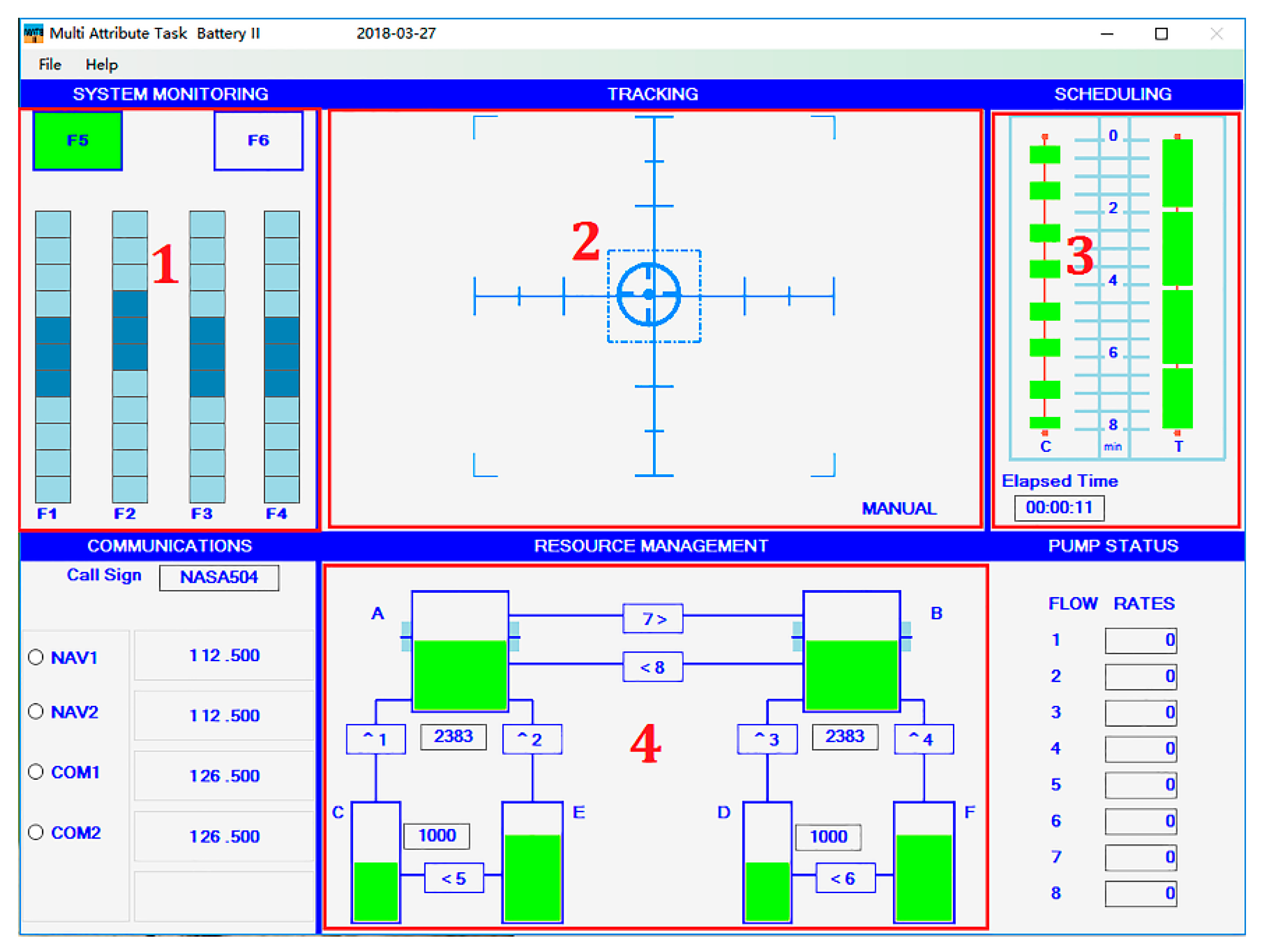
2.2. Experimental Platform

This experiment uses the Multi Attribute Task Battery II (MATB-II) platform developed by NASA based on multi-task aviation situation operation. Four tasks are performed through the human–computer interaction with MATB-II platform using PXN flight joystick, keyboard, and mouse. The MATB-II platform and task interface are shown in Figure 1.

Figure 1. MATB platform and T-shaped area of interest.

The three experimental levels designed in this experiment are low load, moderate load, and overload. Different load levels are set by the occurrence probability of different subtasks. In order to balance the practice and fatigue effect, the experiment uses the Latin square design to set the experimental processing sequence, balance the experimental conditions, and cancel out the sequence error caused by the influence of the sequence of experimental processing. The experimental task design is shown in Table 1.

Table 1. Experimental task design.

Task	Description	Presentation Frequency (Number Of Operations Required within 5 Min)
		Low Load	Moderate Load	High Load
System monitoring task	Monitor the status of the upper left system monitoring task, and click the corresponding position with the mouse to respond.	1	12	24
Tracking monitoring tasks	Monitor the upper and middle tracking monitoring task status and position information, press the button to respond, control the joystick.	1	12	24
Communication monitoring task	Monitor the right communication monitoring taskbar and upcoming communication tasks, and press the button to respond.	1	12	24
Resource management task	Monitor the middle and lower resource management tanks A, B, C, D oil status and oil pump failure information.	1	12	24

2.3. Experimental Procedure

The resting task and three formal experiments with different loads are carried out in the order of the Latin square design. The experimental procedure is shown in Table 2.

Table 2. Experimental flow chart.

Experimental Stage	Experimental Operation	Time-Consuming (Minutes)
1. Experimental training	Read the lab guide, flight simulation mission training	20
2. Debugging physiological equipment	Debug EEG acquisition system and experimental preparation	30
3. Resting task	Rest 3min task (blinking, closed eye activity)	5
4. Formal experiment 1	Carry out the first load level experiment	25
5. Fill in the form and rest	Fill in the 3D-SART scale, NASA-TLX scale, rest	15
6. Formal experiment 2	Carry out the second load level experiment	25
7. Fill in the form and rest	Fill in the 3D-SART scale, NASA-TLX scale, rest	10
8. Formal experiment 3	Carry out the third load level experiment	25
9. Fill in the form	Fill in the 3D-SART scale, NASA-TLX scale	5
10. Fill in the form	NASA-TLX weight check, task attribute comparison score	10

2.4. Data Acquisition

The experimental data were collected in three aspects: subjective evaluation scale, operational performance measurement system, and physiological collection system.

2.4.1. Subjective Rating Scale

The subjective evaluation scale used in this experiment is the National Aeronautics and Space Administration-Task Load Index (NASA-TLX) scale. In order to measure the value of the brain load from the actual feelings and viewpoints of the operators themselves, the subjects are evaluated in the six dimensions of mental power demand, physical strength demand, time demand, effort level, performance level, and frustration degree. The weights of each dimension are determined by a two-two comparison method, and the final mental load value is calculated by a weighted average method.

The statistical results show that the NASA-TLX score gradually increases with the increase of mental load in the experimental design. Analysis of variance by SPSS repeated measurements shows that the main effect of NASA-TLX scores is significant for brain load factors (F (2, 44) = 51.651, p < 0.001, η²_P = 0.701). Post-hoc least significance difference (LSD) analysis shows that the low-load NASA-TLX score is significantly lower than the medium load (p < 0.001) and high load (p < 0.001), while the medium-load NASA-TLX score is significantly lower than the high load (p < 0.001). Considering the effectiveness of the NASA-TLX scale for assessing mental workload, it is shown that the workload task conditions in the experiment are well set-up.

2.4.2. The Operational Performance Measurement System

The flight performance data is automatically recorded by the MATB-II platform in the background. The recorded contents are the correctness rate and response time of each task which are used to evaluate the subject’s understanding of the experiment requirements or the serious attitude to the experiment. The final analysis of the data is based on the operational performance.

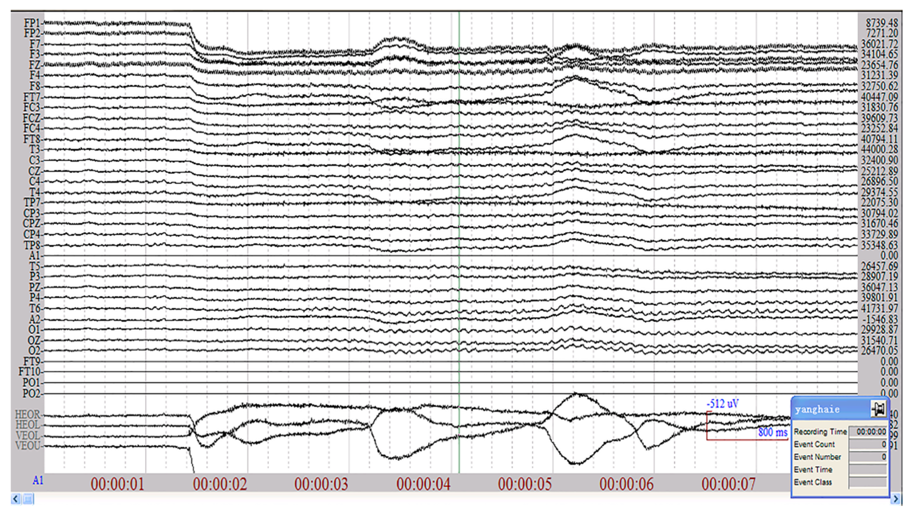
2.4.3. Physiological Acquisition System

This experiment used the Neuroscan Neuamps system (Synamps2, Scan4.3, EI Paso, TX, USA) to acquire a 32-lead EEG signal at a sampling rate of 1000 Hz and recorded a 4-lead vertical and horizontal EOG as well. The layout of the 32-lead electrode is shown in Figure 2.

Figure 2. Thirty-two electrode arrangement.

Taking the subject 5 under low load as an example, part of the EEG raw data is shown in Figure 3, and it can be seen that the EEG signal is a non-stationary random signal.

Figure 3. Part of the original EEG signal of the subject 5 under low load.

3. Data Analysis Method

In this section, the proposed EEG data processing and classification analysis methods are presented. First, the EEG data is preprocessed according to the two criteria of “high performance” and “fewer artifacts” for subsequent analysis; then feature extraction is performed by calculating the power spectral density and energy. After preprocessing and feature extraction of EEG signals, the importance rating of EEG is evaluated by calculating the Gini index, and the most sensitive band under different mental loads is selected. Finally, the EEG signals are classified by the SVM classifier according to the most sensitive band and full band data. A detailed introduction is described in the following sections.

3.1. Data Preprocessing Method

Independent Component Analysis

(1) Principle

The noise-free model of ICA used for eliminating artifacts is represented by Figure 4, and the relationship can be expressed by Equation (1):

$$x=AS$$

(1)

where $A\in R^{N\ast M}$ is the signal transfer matrix, x is the N-dimensional observation vector, and S is the M-dimensional (N ≥ M) original signal. Independent component analysis is to design a matrix W to find $y=Wx$ and solve the independent components y. We remove y’ by one or a part of the component of y, which is represented by $y’=py$. Then $x’=Ay’$ is restored, where x’ is the useful signal left after we eliminate the interference. It can be seen from the model that ICA estimates the source component S_i from the mixed signal x = (x₁, x₂, ..., x_n) and the mixing matrix A as well. It is based on statistically independent signals from different sources.

Figure 4. Independent component analysis eliminates the artifact model.

(2) Description of the ICA issue

Due to the statistically independent conditions of the source signal, it can be separated from the mixed signal, and the separated y(t) components are also independent of each other.

Researchers in this field have proposed different criterias from different application perspectives. Currently, the criterias based on the minimization of mutual information (MMI) and the maximization of entropy are the most widely used. The basic theory is derived from the probability density function of independence. In actual work, the probability density is generally unknown and difficult to estimate. The commonly used method is to expand the probability density as a series and convert it into high-order statistics. The estimation of the high-order statistics, or the introduction of nonlinear links at the output to establish optimization criteria, also implies the pursuit of higher-order statistics. The principle of the criterion is explained by the minimum mutual information criterion.

The minimum mutual information criterion is defined as: Let y be an M-dimensional random variable, p(y) be its probability density, p(y_i) be the edge density of component I in y, then the mutual information entropy of y is defined as:

$$I\left(Py\right)=\int p\left(y\right)log\frac{p(y)}{{\displaystyle \prod p(y_i)}}dy$$

(2)

Obviously, $p\left(y\right)={\displaystyle \prod _{i=1}^{M}p\left(y_i\right)}$, I(p_y) = 0 when it is assumed that the signal source is independent, that is, the components are independent of each other. Therefore, the mutual information is extremely small as a criterion for independent components.

In practical applications, the Kullback–Leibler divergence between p(y) and ${\displaystyle \prod _{i=1}^{M}p\left(y_i\right)}$ is generally used as a quantitative measure of the degree of independence:

$$I\left(y\right)=KL[P\left(y\right),{\displaystyle \prod _{}^{N=i=1}{p}_i\left(y_i\right)}]$$

(3)

$$I\left(y\right)=\int p\left(y\right)log[\frac{P\left(Y\right)}{{\displaystyle \prod _{}^{N=i=1}{p}_i\left(y_i\right)}}]dy$$

(4)

Obviously, I(y) ≥ 0, when each component is independent, I(y) = 0. Therefore, the direct form of the minimum mutual information criterion is: looking for B under y = bx, which is the minimum of I(y) of (3).

In order to be practically usable, the probability density in I(y) needs to be expanded into a series. Since the entropy of the Gaussian distribution is the largest in the probability density distribution with equal covariance, the Gaussian distribution of covariance is commonly used as a reference standard in the expansion. For example, when Gram–Charlier is expanded, there is:

$$\frac{P\left(y_i\right)}{P_G\left(y_i\right)}=1+\frac{1}{3!}{k}_2{y}_i{h}_3\left(y_i\right)+\frac{1}{4}{k}_4{y}_i{h}_4\left(y_i\right)+\dots \dots$$

(5)

where P_G(y_i) is a Gaussian distribution with the same variance (${\delta }^2=1$) and mean ($\mu =0$) as P(y_i), k₃y_i and k₄y_i are third-order and fourth-order statistics of y_i, and h_n(y_i) is n-order Hermit Polynomial.

(3) ICA algorithm solution

Generally, the observed signal is whitened, and the similar principal component analysis method is used to obtain:

In mode: x = As

$$u=Mx=MAs=Bs$$

(6)

In Equation (6) $B=MA$, u is s linearly changed $u=Ms$, it satisfies: $E\left\{x{x}^T\right\}=I$

(4) Separation of independent components

To estimate n independent components, we need to run the algorithm n times. In order to guarantee the different independent components of each separation, it is only necessary to add a simple orthogonal projection operation to the algorithm—the orthogonalization of the mixed matrix columns.

3.2. Feature Extraction Method

Feature extraction is performed by calculating the power spectral density and energy of the EEG data. The corresponding power spectral density (PSD) can be calculated according to Equation (7).

$$p(n)=\frac{F(n)F^{\ast }(n)}{N}$$

(7)

where F*(n) is the conjugate of F(n) and N is the signal length.

Therefore, according to the frequency band distribution of the EEG signal, four energy characteristics corresponding to the four bands are calculated by Equation (8).

The data is normalized using Equation (9).

$$\begin{array}{l}{E}_{\alpha }={\displaystyle \sum _{freq=8}^{13}{p}_{freq}}\\ E_{\beta }={\displaystyle \sum _{freq=14}^{30}{p}_{freq}}\\ E_{\theta }={\displaystyle \sum _{freq=4}^7{p}_{freq}}\\ E_{\delta }={\displaystyle \sum _{freq=0.5}^3{p}_{freq}}\end{array}$$

(8)

where P_freq refers to the power spectral density value at a certain frequency value.

$$x’=\frac{x-x_{\min }}{x_{\max }-x_{\min }}$$

(9)

3.3. Feature Selection Method

Gini Impurity

Gini index: The probability that a randomly selected sample will be misclassified in a subset [28,29]

$$I_G(f)={\displaystyle \sum _{i=1}^m{f}_i(1-f_i)}={\displaystyle \sum _{i=1}^m{f}_i-f_i{}^2=}{\displaystyle \sum _{i=1}^m{f}_i}-{\displaystyle \sum _{i=1}^m{f}_i{}^2}=1-{\displaystyle \sum _{i=1}^m{f}_i{}^2}$$

(10)

where m is the number of classes, and f_i indicates the probability of the samples belonging to the ith class.

Usually, there are hundreds of features in a data set. Selecting several features that have the greatest impact on the results can reduce the number of features when building the model. Here, random forests are used to filter the features. The feature selection is based on the Gini index, and the greater the change in the Gini index before and after the feature selection means that the feature has a greater influence.

The Gini index is expressed by GI and can be calculated according to Equation (10). The variable importance measures are expressed by VIM, and the Gini coefficient score VIM_j ^(Gini) of each feature Xj can be calculated according to Equations (11) and (12).

$$VI{M}_{jm}{}^{(Gini)}={GI}_m-{GI}_l-{GI}_r$$

(11)

$$VI{M}_j{}^{(Gini)}={\displaystyle \sum _{i=1}^{n}VI{M}_{ij}{}^{(Gini)}}$$

(12)

where GI_m, GI_l, and GI_r respectively represent the Gini index before branching and the Gini index of the two new nodes after branching in random forests.

3.4. SVM Classifier

3.4.1. Description

SVM is a classification model whose basic model is a linear classifier that defines the largest interval in the feature space. By incorporating a kernel function, the SVM can be a substantially nonlinear classifier. The learning strategy of SVM is to maximize the interval and can be formalized as a problem of solving convex quadratic programming. For the nonlinear SVM, the classification decision function is learned from the nonlinear classification training set, through the kernel function and soft interval maximization, or convex quadratic programming.

$$f\left(x\right)=\mathrm{sign}\left({\displaystyle \sum _{i=1}^N{a}_i^{*}{y}_{i}K(x,x_i)+b^{*}}\right)$$

(13)

The f(x) obtained by Equation (14) is called a nonlinear support vector, and K(x, z) is a positive definite kernel function.

3.4.2. Kernel Function

The choice of SVM kernel functions is crucial for the classification performance, especially for linearly inseparable data. The kernel function chosen here is the Gaussian kernel function.

$$K\left(x,z\right)=\exp \left(-\frac{{\Vert x-z\Vert }^2}{2{\sigma }^2}\right)$$

(14)

The corresponding support vector machine is a Gaussian radial basis function classifier. In this case, the classification decision function becomes

$$f\left(x\right)=\mathrm{sign}\left({\displaystyle \sum _{i=1}^{N_s}{a}_i^{*}{y}_i\exp \left(-\frac{{\Vert x-z\Vert }^2}{2{\sigma }^2}\right)+b^{*}}\right)$$

(15)

4. Significance Analysis of Mental Workload and Feature Based on SVM Classifier

4.1. Data Preprocessing

In order to ensure the validity of the experimental data, only the experimental data of 10 subjects is left for subsequent analysis according to the two criteria of “high performance” and “fewer artifacts” [30]. The “high performance” criterion means that the operational performance accuracy rate should be greater than 0.90. “Fewer artifacts” means that the artifacts in the original EEG data cannot exceed 5 min. EEG signals are very weak, and EMG, EOG, and ECG can interfere with EEG signals, so samples with artifacts greater than 5 min are removed. After that, the ICA is used to remove the EOG artifacts from the valid 10 subjects, and then filter and reconstruct the reference.

ICA-Based EEG Signal EOG Elimination

The applicable conditions of ICA are: (1) There is no time delay for the linear combination of signals; (2) the time course of the source is independent; and (3) the number of sources is smaller than or equal to the number of sampling points. EEG acquisition can be regarded as linear and immediate, by satisfying condition (1). Condition (2) is also reasonable, because it can be considered that EEG, ECG, EEG, etc., have different sources. Condition (3) is a bit fuzzy because we do not know the number of sources that are statistically independent of scalp potential, but a large number of ICA algorithm simulations can effectively separate a large number of time-dependent sources of EEG or brain topography.

We input the EEG signal (x) as the data sampled from different electrodes and x = As. By the fast fixed-point ICA algorithm we can find A, s. Then the artifacts can be eliminated to get s’.

$$x’=W^{-1}s’$$

(16)

Through (16), the EEG signal x’ can be obtained after removing the eye electricity.

Figure 5 shows the EEG topographic map of the subject 5 under low load, moderate load, and overload before the artifact is removed.

Figure 5. Subject 5 uses ICA to remove artifacts before EEG topographic map.

Figure 6 shows the EEG topographic map of the subject 5 under low load, moderate load, and overload after removing the artifact through ICA.

Figure 6. Subject 5 uses ICA to remove artifacts after EEG topographic map.

Figure 7 shows the EEG topographical map of the subject 12 under low load, moderate load, and overload before using ICA to remove artifacts.

Figure 7. Subject 12 uses ICA to remove artifacts before EEG topographic map.

Figure 8 shows the EEG topographic map of the energy of the subject 12 under low load, moderate load, and overload after using the ICA to remove artifacts.

Figure 8. Subject 12 uses ICA to remove artifacts after EEG topographic map.

It can be seen from Figure 6 and Figure 8 that the individual brain activities are distinct under different load conditions.

4.2. Feature Extraction

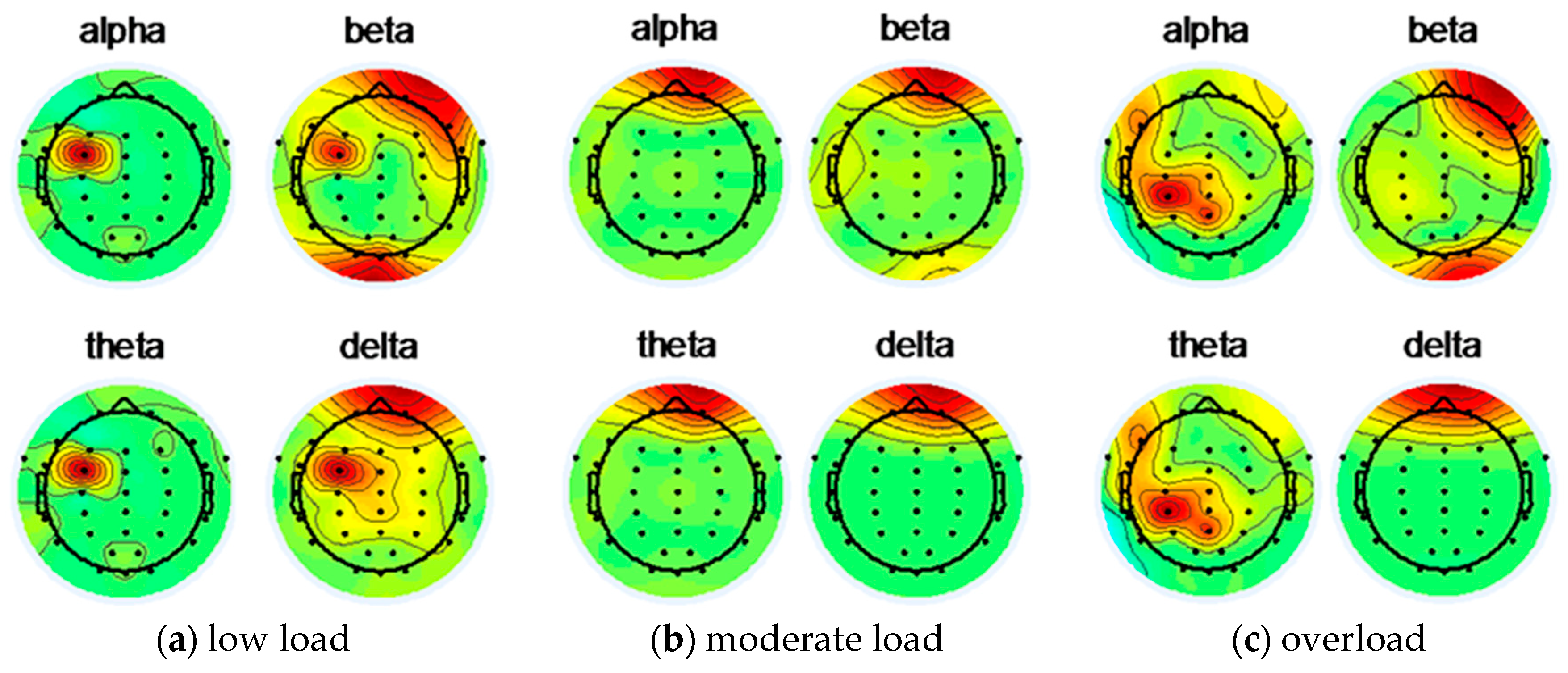
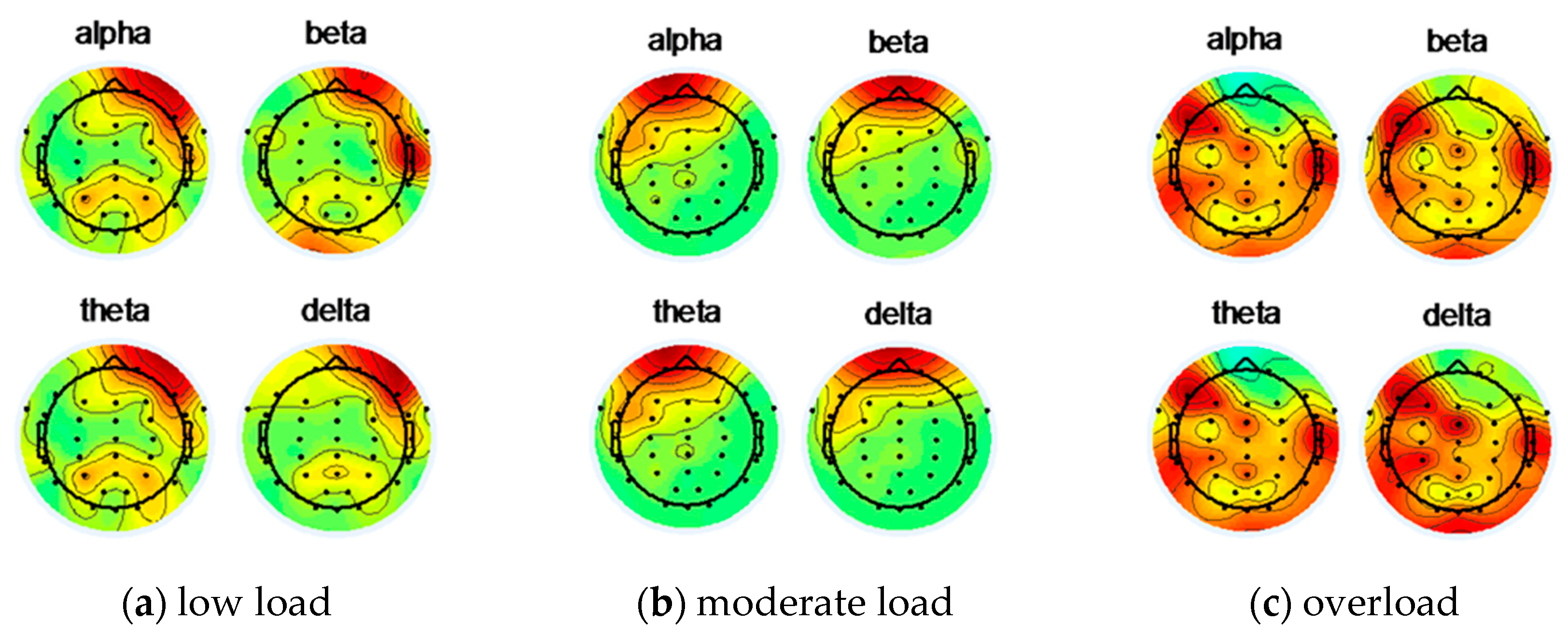
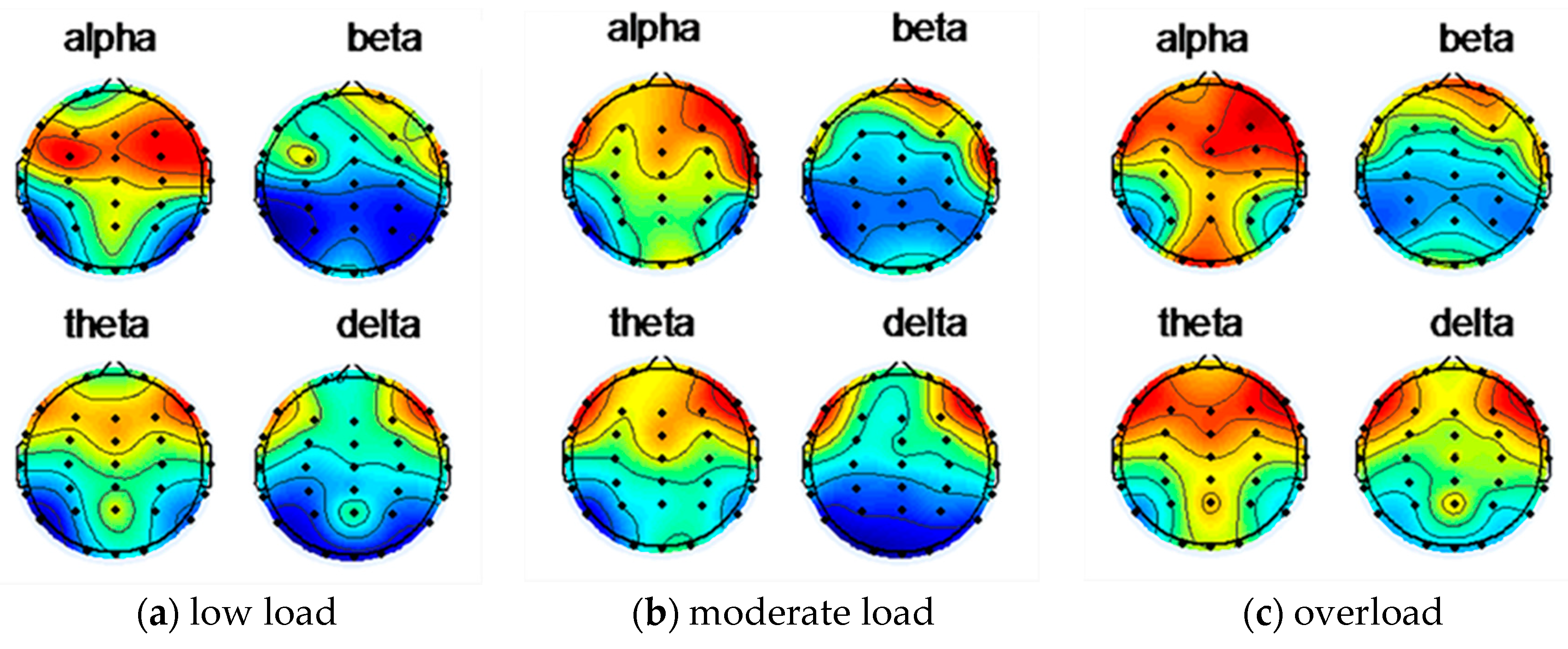
4.2.1. Four Bands of EEG Data

Numerous studies have shown that human brain states are related to the α, β, θ, and δ bands.

α band: The electromagnetic wave frequency is between 8~13 Hz, and the amplitude is between 30~50 μV. This periodic wave is produced in the parietal lobe and occipital region of the brain in the state of consciousness, quietness, or rest.

β band: The electromagnetic wave frequency is between 14~30 Hz, and the amplitude is between 5~20 μV. This activity occurs in the frontal area when people are awake and alert.

θ band: An electromagnetic wave with a frequency between 4 and 7 Hz with an amplitude of less than 30 μV. This activity occurs mainly in the parietal and temporal regions of the brain.

δ band: The electromagnetic wave frequency is between 0.5~3 Hz, and the amplitude is between 100~200 μV. This activity occurs during deep sleep, unconsciousness, anesthesia, or hypoxia.

4.2.2. Feature Extraction Based on Power Spectral Density and Energy

To minimize the time effects, EEG data of the middle 5 min is selected. Segmentation processing, fast Fourier transformation, power spectrum estimation, and energy calculation are performed in sequence. When segmentation is performed, the length of each segment is 1 s. Based on the idea of the averaging period method, half of the adjacent segments data is overlapped making the EEG characteristic curve smoother. Then, the Fourier transformation is performed on each segment to obtain F(n) (n = 1, 2, ..., 1000), and the corresponding frequency and amplitude.

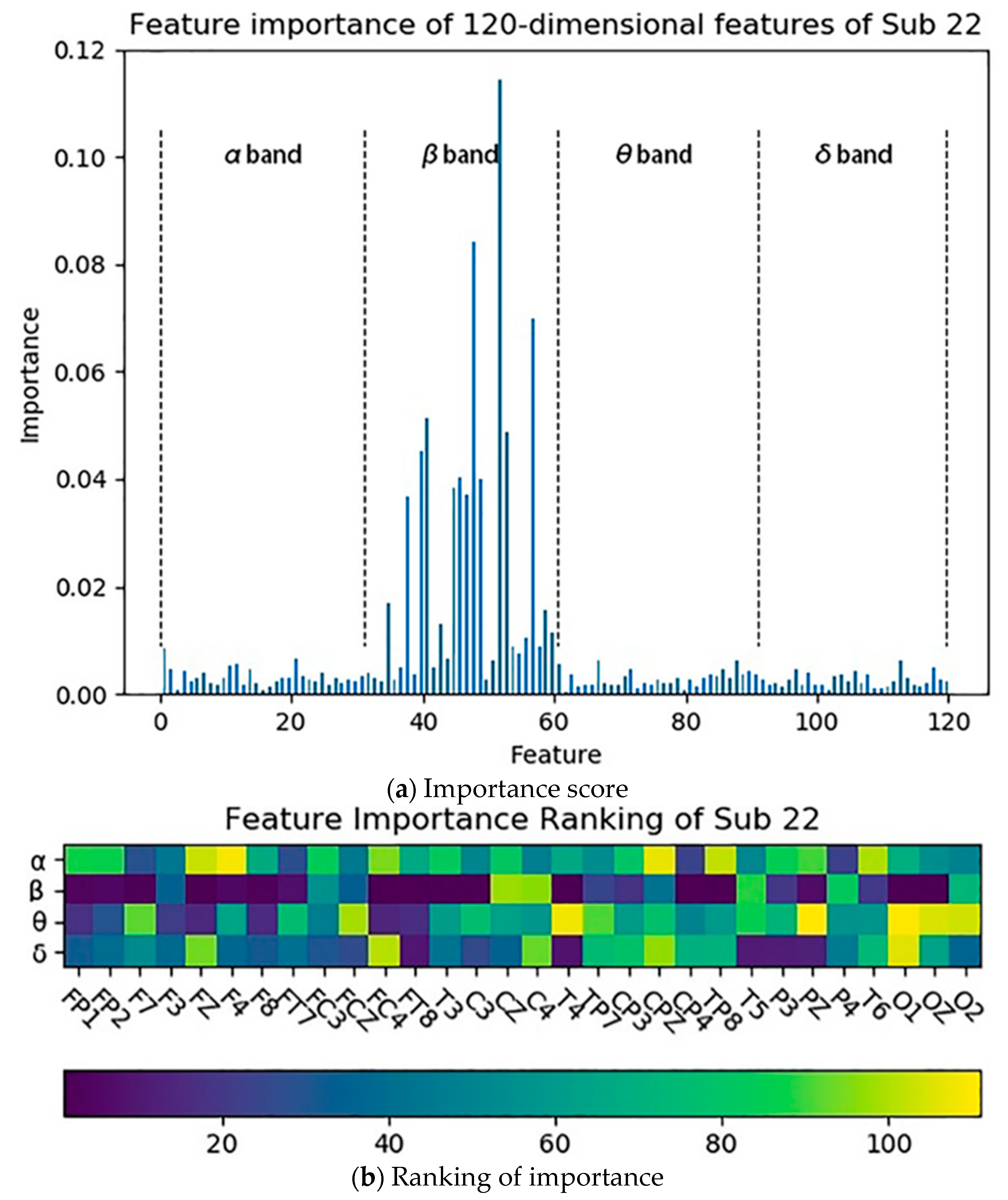
4.3. Feature Selection Based on Gini Impurity

The 120-dimensional characteristic distribution of EEG data is: 1–30 dimension is the α band of each electrode point, 31–60 dimension is the β band of each electrode point, 61–90 dimension is the θ band of each electrode point, 91–120 dimension is the δ band of each electrode point. Taking the subject 22 as an example, the importance distribution of the 120-dimensional features in the EEG data calculated by Gini’s impurity is shown in Figure 9.

Figure 9. The importance distribution of the 120-dimensional features of the subject 22: (a) describes the importance scores of the individual features; (b) describes the ranking of the individual features according to the importance scores.

It can be seen from Figure 9 that the features with higher importance are concentrated in the β band of each electrode point, and the β band plays a major role in the four bands. The results obtained by performing the same feature selection for the remaining subjects are shown in Figure 10. It can be found that the features with higher importance in the EEG are also concentrated in the β band, which means the β band is the most sensitive compared to other bands.

Figure 10. Distribution of importance of the 120-dimensional features of the remaining subjects: (a) describes the importance scores of each feature of the remaining subjects; (b) describes the ranking of the characteristics of the remaining subjects according to the importance score.

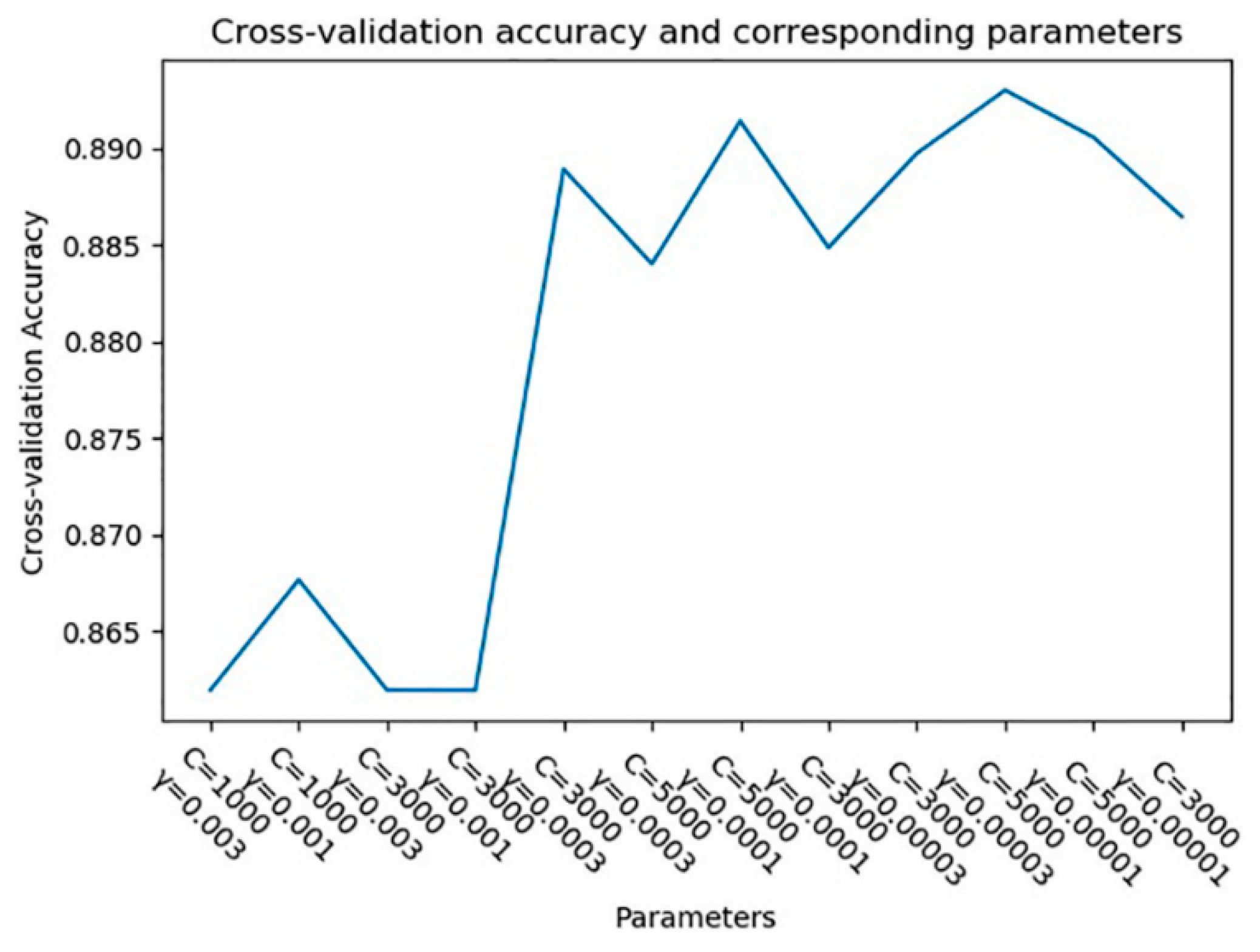
4.4. Application of SVM Classifier to EEG Signals

Considering the individual differences, a load classification model for each subject is established separately. The following is an example of subject 22 to illustrate the construction of the classification network. The classification data set information after feature extraction and feature selection are shown in Table 3. The data volume and data dimension of different loads, training set, cross-validation set, and test set are given in the table.

Table 3. Classification data set after feature extraction and feature selection.

	Data	Low Load	Moderate Load	High Load	Training Set	Cross-Validation Set	Test Set
After Feature Extraction	number	583	583	583	1224	122	525
	dimension	120	120	120	120	120	120
After Feature Selection	number	583	583	583	1224	122	525
	dimension	30	30	30	30	30	30

The dataset of subject 22 obtained in Section 4.2 can be expressed as A₁, A₂, ..., A₁₇₄₉. Each dataset has 120 dimensions, where the low load tag is 0, the moderate load tag is 1, and the high load tag is 2. Since the sample size of each load level is 583, the effective number of samples of this model is 1749.

The input information of all feature data when using the SVM classifier is

$${[X_{d1}^{}]}_{\mathrm{mod}1}=\left[\begin{array}{l}{\left[A_1\right]}^1,\dots ,{\left[A_1\right]}^{120}\\ {\left[A_2\right]}^1,\dots ,{\left[A_2\right]}^{120}\\ \hfill \dots \hfill \\ {\left[A_{1749}\right]}^1,\dots ,{\left[A_{1749}\right]}^{120}\end{array}\right]$$

$${[Y_{d1}]}_{\mathrm{mod}1}={\left(0^1,\dots ,0^{583},1^1,\dots ,1^{583},2^1,\dots ,2^{583}\right)}^T$$

The input information of the β band feature data when using the SVM classifier is

$${[X_{d1}^{}]}_{\mathrm{mod}1}=\left[\begin{array}{l}{\left[A_1\right]}^{31},\dots ,{\left[A_1\right]}^{60}\\ {\left[A_2\right]}^{31},\dots ,{\left[A_2\right]}^{60}\\ \hfill \dots \hfill \\ {\left[A_{1749}\right]}^{31},\dots ,{\left[A_{1749}\right]}^{60}\end{array}\right]$$

$${[Y_{d1}]}_{\mathrm{mod}1}={\left(0^1,\dots ,0^{583},1^1,\dots ,1^{583},2^1,\dots ,2^{583}\right)}^T$$

The training set and the test set are randomly divided by 70%:30%. After the classification network is adjusted to the appropriate parameters, the network training is completed.

The SVM model has two very important parameters C and γ. Where C is the penalty factor, which is the tolerance for the error. The higher the C value is, smaller error can be allowed, and the over-fitting occurs more easily. The smaller the C value is, the easier under-fitting occurs. If the C value is too large or too small, the generalization ability is poor. γ implicitly determines the distribution of data after mapping to a new feature space. The larger the γ is, the more vectors there are. The number of support vectors affects the speed of training and prediction. So the two critical parameters of the classification network are the C and γ value.

Here, the parameters are adjusted according to the accuracy of the cross-validation set, using k-fold cross-validation. We use 10-fold cross-validation since it is the most widely used. The average of 10 results is used as an indicator, and a single estimation is finally obtained. This ensures that each subsample participates in the training and test, reducing generalization errors and preventing overfitting.

Taking the subject 22 as an example, the accuracy of the cross-validation set under different parameters is shown in Figure 11. It can be seen from the figure that when C = 5000 and γ = 0.00003, the accuracy of the cross-validation set is the highest.

Figure 11. Cross-validation accuracy and corresponding parameters.

The classification result confusion matrix is used to reflect the quality of the classification results. Taking the three classifications as an example, the layout of the confusion matrix is shown in Table 4.

Table 4. Confusion matrix layout

Target Class	M00	M01	M02
	M10	M11	M12
	M20	M21	M22
Output Class

M_ij (i = 0, 1, 2, j = 0, 1, 2) indicates the number of samples in which the i-th class is divided into the j-th class. Among them, if i = j, the classification is correct, and if i ≠ j, the classification is wrong. From this indicator, the difficulty degree of classification can be determined.

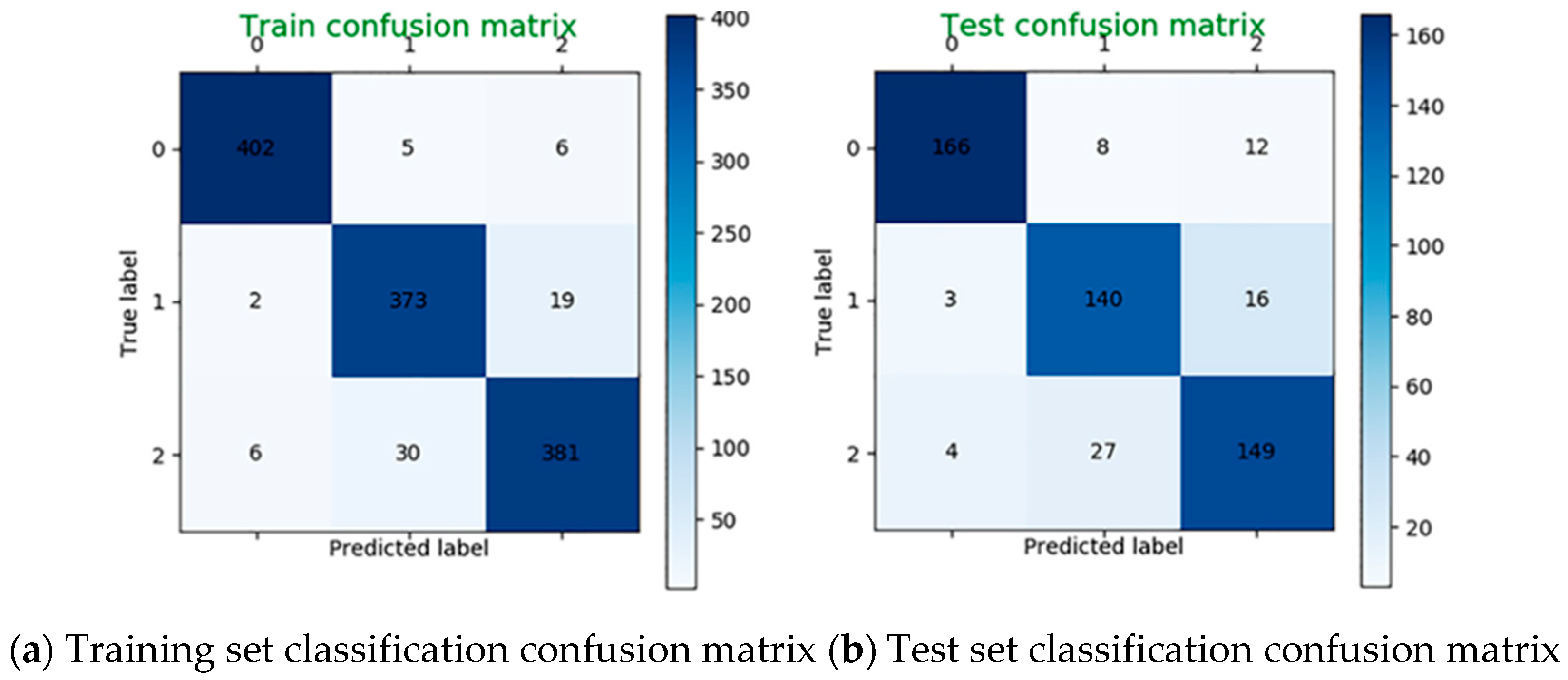
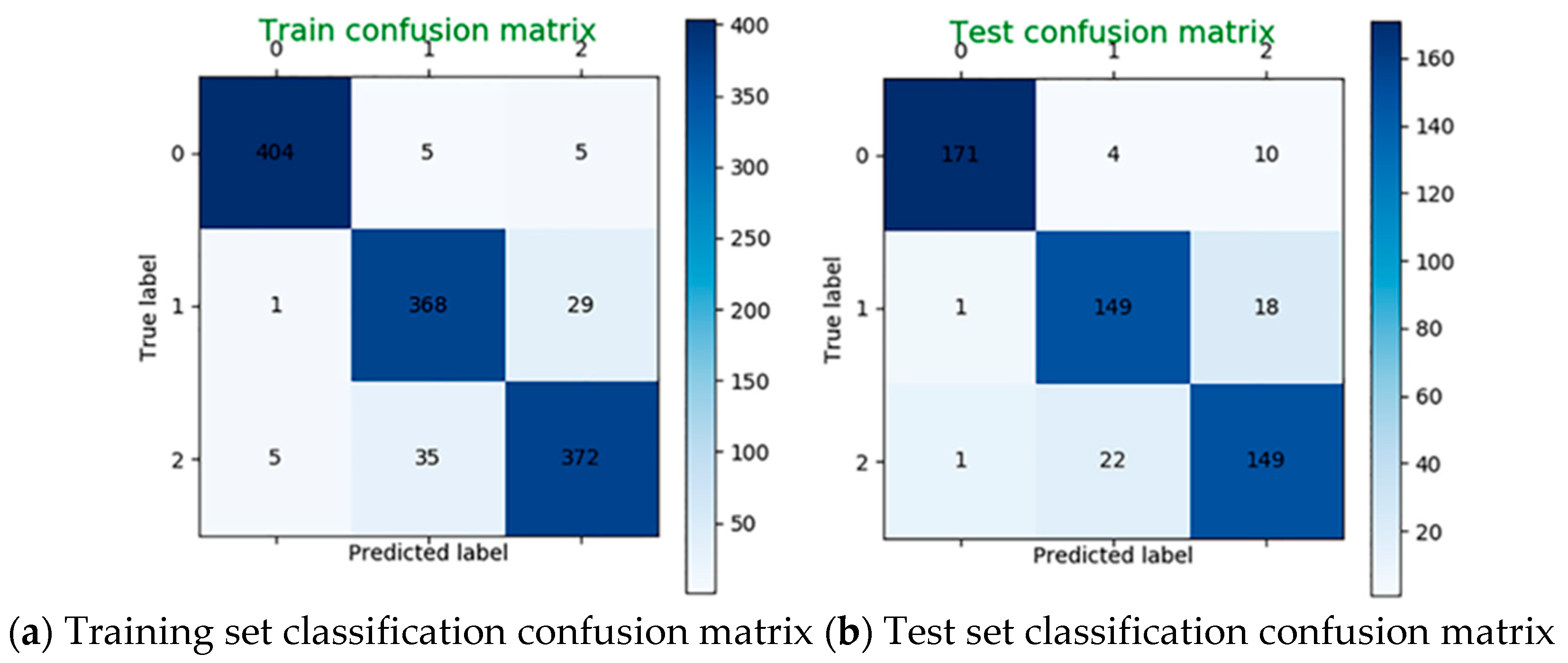
4.5. Classification Result of All Feature Data

The SVM is used to classify the mental load for the data in the four bands. Taking the subject 22 as an example, when C = 5000, γ = 0.00003, the classification accuracy is 94% on the training set and 87% on the test set. The classification confusion matrix is shown in Figure 12.

Figure 12. Classification confusion matrix using four bands data.

4.6. Classification Result of β Band Feature Data

The SVM is also applied to classify the mental load for the β band characteristic data. Taking the subject 22 as an example, when C = 100, γ = 0.03, the classification accuracy is 93% on the training set and 89% on the test set. The classification confusion matrix is shown in Figure 13.

Figure 13. Classification confusion matrix using β band data alone.

4.7. Comparative Analysis of Classification Results

The full band and β band features of all the participants are sent to the SVM for classification of mental load respectively. The classification accuracy of the two methods on the test set is shown in Table 5, where Acc(f) indicates the accuracy of classification using full band features, and Acc(β) indicates the accuracy of classification using the β band feature.

Table 5. Classification accuracy of the four band features and the β band feature on the test set (unit: %).

Subject Number	Acc(f)	Acc(β)	Acc(β) − Acc(f)
Subject 01	72	73	+1
Subject 02	72	74	+2
Subject 05	87	86	−1
Subject 06	90	93	+3
Subject 07	89	91	+2
Subject 08	77	77	0
Subject 10	79	81	+2
Subject 12	96	96	0
Subject 18	91	92	+1
Subject 22	87	89	+2

From the classification results, the effect of using the β band data for classification alone is better than the classification using the four bands data. It can be explained that the β band feature contains most of the useful information about the data. The rest of the band information interferes with the data. In the case of testing mental load, the β band data can be separately analyzed, which not only can reduce the dimension of the data, but can also improve the performance of the model, and save resources such as memory.

5. Conclusions

In this paper, the sensitive bands of EEG data under different mental workloads are studied. The signals are obtained through different flight load experiments. Feature extraction is performed by calculating the PSD and energy of the EEG signal. According to the feature selection of Gini impurity, the importance index of different bands of EEG data is analyzed using the Gini index, and the characteristics of the band with higher importance are obtained. It is found that the β band has the highest importance and sensitivity under different mental loads. The data of the four bands and the data of the separate β band are sent to the SVM classifier for verification. By observing the final classification accuracy, it is found that the data of the β band alone has higher final classification accuracy than the data of the four bands. This also shows that the β band data is more important and sensitive than other bands under different brain loads, and can represent the entire EEG data for subsequent data analysis.

References

- Schalk, G.; McFarland, D.J.; Hinterberger, T.; Birbaumer, N.; Wolpaw, J.R. BCI2000: A General-Purpose Brain-Computer Interface (BCI) System. IEEE Trans. Biomed. Eng. 2004, 51, 1034–1043. [Google Scholar] [CrossRef] [PubMed]
- Cavazza, M. A Motivational Model of BCI-Controlled Heuristic Search. Brain Sci. 2018, 8, 166. [Google Scholar] [CrossRef] [PubMed]
- Hosseini, M.-P.; Pompili, D.; Elisevich, K.; Soltanian-Zadeh, H. Optimized Deep Learning for EEG Big Data and Seizure Prediction BCI via Internet of Things. IEEE Trans. Big Data 2017, 3, 392–404. [Google Scholar] [CrossRef]
- Heilinger, A.; Guger, C. EEG-Trockenelektroden und ihre Anwendungen bei BCI-Systemen. Das Neurophysiol.-Labor 2019. [Google Scholar] [CrossRef]
- Lin, C.-J.; Hsieh, M.-H. Classification of mental task from EEG data using neural networks based on particle swarm optimization. Neurocomputing 2009, 72, 1121–1130. [Google Scholar] [CrossRef]
- De Haan, W.; Pijnenburg, Y.A.; Strijers, R.L.; van der Made, Y.; van der Flier, W.M.; Scheltens, P.; Stam, C.J. Functional neural network analysis in frontotemporal dementia and Alzheimer’s disease using EEG and graph theory. BMC Neurosci. 2009, 10, 101. [Google Scholar] [CrossRef]
- Radüntz, T.; Scouten, J.; Hochmuth, O.; Meffert, B. Automated EEG artifact elimination by applying machine learning algorithms to ICA-based features. J. Neural Eng. 2017, 14, 046004. [Google Scholar] [CrossRef]
- Croce, P.; Zappasodi, F.; Marzetti, L.; Merla, A.; Pizzella, V.; Chiarelli, A.M. Deep Convolutional Neural Networks for feature-less automatic classification of Independent Components in multi-channel electrophysiological brain recordings. IEEE Trans. Biomed. Eng. 2019. [Google Scholar] [CrossRef]
- Hasasneh, A.; Kampel, N.; Sripad, P.; Shah, N.J.; Dammers, J. Deep Learning Approach for Automatic Classification of Ocular and Cardiac Artifacts in MEG Data. J. Eng. 2018, 2018, 1350692. [Google Scholar] [CrossRef]
- Dharwarkar, G.S.; Basir, O. Enhancing Temporal Classification of AAR Parameters in EEG single-trial analysis for Brain-Computer Interfacing. In Proceedings of the 2005 IEEE Engineering in Medicine and Biology 27th Annual Conference, Shanghai, China, 1–4 September 2005; pp. 5358–5361. [Google Scholar]
- Zhang, A.; Yang, B.; Huang, L. Feature Extraction of EEG Signals Using Power Spectral Entropy. In Proceedings of the 2008 International Conference on BioMedical Engineering and Informatics, Sanya, China, 28–30 May 2008; pp. 435–439. [Google Scholar]
- Kottaimalai, R.; Rajasekaran, M.P.; Selvam, V.; Kannapiran, B. EEG signal classification using Principal Component Analysis with Neural Network in Brain Computer Interface applications. In Proceedings of the 2013 IEEE International Conference ON Emerging Trends in Computing, Communication and Nanotechnology (ICECCN), Tirunelveli, India, 25–26 March 2013; pp. 227–231. [Google Scholar]
- Subasi, A. EEG signal classification using wavelet feature extraction and a mixture of expert model. Expert Syst. Appl. 2007, 32, 1084–1093. [Google Scholar] [CrossRef]
- Jahankhani, P.; Kodogiannis, V.; Revett, K. EEG Signal Classification Using Wavelet Feature Extraction and Neural Networks. In Proceedings of the IEEE John Vincent Atanasoff 2006 International Symposium on Modern Computing (JVA’06), Sofia, Bulgaria, 3–6 October 2006; pp. 120–124. [Google Scholar]
- Srinivasan, V.; Eswaran, C.; Sriraam, N. Approximate Entropy-Based Epileptic EEG Detection Using Artificial Neural Networks. IEEE Trans. Inform. Technol. Biomed. 2007, 11, 288–295. [Google Scholar] [CrossRef]
- Hyekyung, L.; Seungjin, C. PCA+HMM+SVM for EEG pattern classification. In Proceedings of the Seventh International Symposium on Signal Processing and Its Applications 2003, Paris, France, 1–4 July 2003; Volume 1, pp. 541–544. [Google Scholar]
- Orhan, U.; Hekim, M.; Ozer, M. EEG signals classification using the K-means clustering and a multilayer perceptron neural network model. Expert Syst. Appl. 2011, 38, 13475–13481. [Google Scholar] [CrossRef]
- Trujillo-Barreto, N.J.; Aubert-Vázquez, E.; Valdés-Sosa, P.A. Bayesian model averaging in EEG/MEG imaging. NeuroImage 2004, 21, 1300–1319. [Google Scholar] [CrossRef]
- Baldwin, C.L.; Penaranda, B.N. Adaptive training using an artificial neural network and EEG metrics for within- and cross-task workload classification. NeuroImage 2012, 59, 48–56. [Google Scholar] [CrossRef] [PubMed]
- Acharya, U.R.; Oh, S.L.; Hagiwara, Y.; Tan, J.H.; Adeli, H. Deep convolutional neural network for the automated detection and diagnosis of seizure using EEG signals. Comput. Biol. Med. 2018, 100, 270–278. [Google Scholar] [CrossRef] [PubMed]
- Richhariya, B.; Tanveer, M. EEG signal classification using universum support vector machine. Expert Syst. Appl. 2018, 106, 169–182. [Google Scholar] [CrossRef]
- Saccá, V.; Campolo, M.; Mirarchi, D.; Gambardella, A.; Veltri, P.; Morabito, F.C. On the Classification of EEG Signal by Using an SVM Based Algorithm. In Multidisciplinary Approaches to Neural Computing; Esposito, A., Faudez-Zanuy, M., Morabito, F.C., Pasero, E., Eds.; Springer International Publishing: Cham, Switzerland, 2018; Volume 69, pp. 271–278. [Google Scholar]
- Clark, I.; Biscay, R.; Echeverría, M.; Virués, T. Multiresolution decomposition of non-stationary eeg signals: A preliminary study. Comput. Biol. Med. 1995, 25, 373–382. [Google Scholar] [CrossRef]
- Moretti, D.V.; Babiloni, C.; Binetti, G.; Cassetta, E.; Dal Forno, G.; Ferreric, F.; Ferri, R.; Lanuzza, B.; Miniussi, C.; Nobili, F.; et al. Individual analysis of EEG frequency and band power in mild Alzheimer’s disease. Clin. Neurophysiol. 2004, 115, 299–308. [Google Scholar] [CrossRef]
- Liao, X.; Yao, D.; Wu, D.; Li, C. Combining Spatial Filters for the Classification of Single-Trial EEG in a Finger Movement Task. IEEE Trans. Biomed. Eng. 2007, 54, 821–831. [Google Scholar] [CrossRef]
- Saby, J.N.; Marshall, P.J. The Utility of EEG Band Power Analysis in the Study of Infancy and Early Childhood. Dev. Neuropsychol. 2012, 37, 253–273. [Google Scholar] [CrossRef]
- Trejo, L.J.; Kochavi, R.; Kubitz, K.; Montgomery, L.D.; Rosipal, R.; Matthews, B. Measures and Models for Predicting Cognitive Fatigue. In Proceedings of the Defense and Security, Orlando, FL, USA, 23 May 2005; p. 105. [Google Scholar]
- Raileanu, L.E.; Stoffel, K. Theoretical Comparison between the Gini Index and Information Gain Criteria. Ann. Math. Artif. Intell. 2004, 41, 77–93. [Google Scholar] [CrossRef]
- Strobl, C.; Boulesteix, A.-L.; Augustin, T. Unbiased split selection for classification trees based on the Gini Index. Comput. Stat. Data Anal. 2007, 52, 483–501. [Google Scholar] [CrossRef]
- Vigario, R.; Sarela, J.; Jousmiki, V.; Hamalainen, M.; Oja, E. Independent component approach to the analysis of EEG and MEG recordings. IEEE Trans. Biomed. Eng. 2000, 47, 589–593. [Google Scholar] [CrossRef] [PubMed]
© 2019 by the authors. Licensee MDPI, Basel, Switzerland. This article is an open access article distributed under the terms and conditions of the Creative Commons Attribution (CC BY) license (http://creativecommons.org/licenses/by/4.0/).