1. Introduction
During the last few decades, interval analysis has been shown to provide efficient numerical approaches for solving various tasks in scientific computing, as well as in application-oriented disciplines in which numerical techniques with a result verification are helpful or required. In such a way, they help to solve problems in control engineering, robotics, including rigorous methods for localization and/or path planning, as well as guaranteed obstacle avoidance, computational (bio-)mechanics, civil engineering, or bio-engineering, just to mention a few of the large number of different areas [
1,
2,
3,
4,
5,
6,
7].
In these applications, not only the possibility of interval analysis to treat the effects of round-off and truncation errors of numerical solution techniques (such as truncated temporal Taylor series expansions for the solution of initial value problems to ordinary differential equations) is exploited [
8,
9,
10]. In addition, these applications also benefit from a further fundamental property of interval analysis, namely that it provides guaranteed outer enclosures of all possible solutions to a mathematical problem at hand in the presence of ambiguities in the solutions or in the presence of bounded uncertainty in selected parameters.
Here, a selection of useful techniques ranges from the extension of fundamental arithmetic operations to interval valued expressions [
1,
2,
3], which were recently standardized in the IEEE standard 1788 [
11], over the development of set valued counterparts for zero finding techniques for sets of algebraic equations such as the Krawczyk operator [
12,
13,
14], interval based techniques for reachability analysis [
15], the verified global optimization [
16,
17,
18], to the solution of identification tasks by means of set inversion techniques via interval analysis (e.g., the algorithms set inversion via interval analysis (SIVIA) and problem specific generalizations) [
2,
19]. If control applications are concerned, interval analysis can be applied both to an offline design and verification of control procedures under consideration of feasibility and safety requirements such as input and state constraints and to an online interval evaluation in terms of real-time capable robust control strategies generalizing the ideas of variable-structure control techniques and backstepping [
20,
21,
22,
23,
24,
25]. Further, approaches for the control of systems with input saturations that do not rely on interval analysis were handled, for example, in [
26] and the references therein. In addition to the implementation of robust controllers, also the dual task of interval based state estimation and observer design can be solved; see, for example, [
27,
28,
29,
30,
31,
32].
This paper addresses the following two issues: First, a method for finding a nonlinear state-feedback controller is derived for the exact tracking of predefined paths in the phase-space. These paths are assumed to be described in terms of a sliding surface for a nonlinear dynamic system. Second, this control design procedure is interfaced with techniques from the field of interval analysis that are employed to determine enclosures of the invariant sets of the resulting controlled system in a reliable and computationally efficient way. For a continuous-time system model with the state vector
, a subset
is called positively invariant if the relation
is satisfied for all possible
if
holds [
33]. Due to the fact that we are only interested in a forward-in-time propagation of state trajectories, these sets are briefly called invariant throughout this paper. For the proposed control design, an appropriate Gröbner basis is used to check if the occurring Bézout identity has a solution, such that a controller can be designed that does not contain any structural singularities.
To find the invariant set of the respective closed-loop control system, Lyapunov-like functions are employed, which transform the stability properties of dynamical systems described by a set of ordinary differential equations into inequalities. Those inequalities can be evaluated using interval computation and finally lead to the desired enclosures of the invariant sets to be determined. Note that the proposed technique does not focus on determining invariant sets by using the La Salle invariance theorem. Instead, only temporal derivatives of the aforementioned Lyapunov-like functions are required during the solution procedure.
To depict the examined problem and to distinguish it from a state-of-the-art sliding mode control design [
34,
35,
36,
37,
38,
39], consider a single-input system:
where
is the state vector and
is the evolution function. For simplicity, assume that the input in (
1) is given by the state dependent expression
. The time dependencies of the state vector
and of the control vector
are furthermore not explicitly denoted. Additionally, consider a sliding surface:
For the system model defined in Equation (
1), the control input
u should be found in such a way that the function
, which can be interpreted as a Lyapunov function candidate, decreases monotonically up to the point where perfect tracking of the predefined path (respectively, trajectory) occurs due to
. As a consequence, the state trajectories of the controlled system will converge to an invariant set in which the sliding surface should be contained.
The paper is structured in the following way. Firstly, the general concept of sliding mode approaches for the control design of nonlinear systems is described in
Section 2 with the aim of distinguishing the investigated problem from classical techniques in this field. Then, the proposed novel method for a sliding mode-type controller design is explained in
Section 3 in combination with the use of a Gröbner basis to solve Bézout’s identity.
Section 4 deals with the conditions to be satisfied for an invariant set, which are evaluated numerically by using interval analysis as described in
Section 5. In
Section 6, several applications of the developed method are presented. These applications include cases with sliding surfaces represented by closed curves in the phase space. Moreover, straight line segments are considered as well. In addition, a concluding example is investigated where Bézout’s identity is not solvable. However, the interval based method for enclosing the resulting invariant set of the controlled system can still be employed successfully if a bounded control input for the considered nonlinear system of dimension three is analyzed. Finally, conclusions and an outlook toward future work together with an explanation of how the presented interval technique can be applied to other nonlinear control techniques are given in
Section 7.
2. Classical Sliding Mode Control
The main concept in sliding mode control is to replace an
nth order tracking problem by a stabilization problem of the order
[
40]. Looking at the dynamic system:
the guaranteed stabilizing, variable structure input signal
u is chosen according to:
For that purpose, a switching function
needs to be defined. In classical sliding mode procedures, which are applied to solve trajectory tracking tasks, this switching function is usually composed of the output tracking error and a weighted linear combination of the temporal derivatives of this error signal up to the order
, where
denotes the system’s relative degree [
24]. In the remainder of this section, it is assumed that the relative degree
equals the system order according to
. Then, a stability proof of the closed-loop dynamics can be performed in terms of a square Lyapunov function candidate as was mentioned in the Introduction of this paper.
In general, the switching function
determines under which conditions the input signal of the system changes structurally, so that
u becomes discontinuous across
[
40,
41]. In such a way, the sliding surface, which is defined by
, divides the state space into two mutually disjoint domains where either
or
holds. In those domains, different dynamics of the system occur due to different definitions of the system’s input
u. The sliding surface is included in neither of these subdomains as a trajectory, whereas each point of the sliding surface
has to be accessible by a trajectory from either side [
41]. To make the system converge to the sliding surface, the input has to be chosen in such a way that it always makes the state trajectories approach the sliding surface, i.e., they have to be “pushed” towards
. This phase is called the transient or reaching phase. The possibilities for the design of controllers for this reaching phase can be found, for example, in [
42,
43] and the references therein. Note that the design of the corresponding control for this phase needs to account for input constraints in terms of the limited range of the admissible system inputs
u. If scenarios occur, in which the system input reaches its lower or upper saturation value in such a phase, a careful stability proof is inevitable, cf. [
26].
The next phase, following the completion of the reaching phase, is called sliding mode. The system’s dynamics are then represented by the switching function itself. As mentioned before, this function typically has a lower order than the open-loop system [
38,
39].
Thus, in this state, the system’s dynamic behavior only depends on the parameters included in the switching function, which means that this form of control is not only robust against uncertainties in plant parameters, but also against disturbances satisfying suitable matching conditions (for example, disturbances entering the state Equations (
3) via the same channels as the system inputs
u). From an intuitive point of view, this results from the fact that even if the system leaves the sliding surface slightly, it will immediately return to it, because of the switching-type behavior of the input
u and the proven stability (i.e., attraction property) of the sliding surface.
However, the switching between structurally different inputs as defined in (
4) may lead to a phenomenon called chattering, which implies high control activity and thus leads to a rapid wear of the actuator. In addition, the associated high frequencies may also excite dynamics that were not considered in the model [
40]. Strategies aiming at a reduction of the chattering phenomenon by a stability preserving interval based gain adaptation strategy were investigated in [
20,
21,
22,
23,
24,
25].
To ensure that the system will reach the sliding surface in finite time, the condition:
is typically introduced in a classical sliding mode control synthesis. The inequality (
5) means that the squared distance to the sliding surface has to decrease along all possible trajectories with a constant velocity
. This condition makes the set
an invariant set due to the invariance theorem of La Salle. If this condition is satisfied for the complete state space, the system will always converge to the sliding surface.
To reach the sliding mode, the state dependent controller has to be designed. There are various ways to do that, where we restrict ourselves to one of the available options. To deal with possible singularities in the control law and to avoid them during perfect trajectory tracking in the sliding mode, the input
u is chosen according to the concept of equivalent control. To find the equivalent control
that ensures perfect tracking,
should be valid on the sliding surface in order for
s not to change and thus the system to remain in sliding mode. For a system like (
1) with a (nonlinear) feedback controller
, the time derivative of
is calculated by the following Lie derivative of
in the direction of the vector field
, assuming that
does not explicitly depend on the time variable
t:
To find the equivalent input
, this expression is solved with respect to
u. However, if the system states are not on the sliding surface during the reaching phase,
u should make it converge to
. To ensure this behavior, a further term depending on the sign of
s resulting from the right hand side of (
5) is typically added to the equivalent control
to obtain the overall control signal stated in Equation (
4). This can be achieved by using a sign function (often regularized by means of smooth sigmoid-type expressions) depending on the current value of
[
40,
44].
3. Controller Design
To find the controller for the system model (
1) with a time invariant sliding surface as considered in Equation (
6), the following approach is used, which is similar to the one that can be found in [
45] by setting:
where
. Note that this assumption is not only useful for the classical tracking control problem mentioned in the previous section, but it can also be employed to design control procedures allowing for following paths in the phase space that satisfy the design procedures listed in the following. From a dynamics point of view, the factor
in Equation (
7) can be interpreted as a state dependent decay rate for the convergence of tracking errors towards the desired sliding mode.
With the choice given in Equation (
7),
will be forced towards zero, because the resulting derivative
always has the opposite sign of
, leading to the strict inequality:
With the help of the relation (
7), the control signal can be found in symbolic form. As an example, consider a two-dimensional input affine system of the form:
for which Equation (
7) becomes equal to:
as well as equal to:
The latter expression can now be solved for the control input according to:
To avoid singularities in the controller and in this way in the closed-loop system dynamics, the following condition has to be satisfied:
so that all fractions in the expression for the input
u cancel out analytically. After simple rearrangement, this expression becomes:
which is Bézout’s identity, where
and
have to be found in terms of non-singular analytic (polynomial) expressions.
Remark 1. The design procedure summarized above is more general than the classical sliding mode design, where the goal of tracking sufficiently smooth reference trajectories for the desired temporal evolution of the state variable would lead to the system input: Here, the parameter α is chosen as a positive constant (generally satisfying the Hurwitz criterion [20,22]) to ensure stability on the sliding surface and ensures a stable motion during the reaching phase towards the classical (time varying) sliding surface: To solve the Bézout identity (
14) in the design procedure suggested in this paper, it has to be checked firstly whether a solution for this polynomial equation exists. This can be done using a reduced Gröbner basis. If a polynomial belongs to an ideal, it can be expressed as a linear combination of the polynomials that belong to the generating set of the ideal in a polynomial ring. This means if the term:
included in the system input defined in Equation (
12) is part of the ideal:
Equation (
14) has a solution.
The Gröbner basis can provide this generating set of polynomials, and the reduced Gröbner basis makes sure that none of the leading coefficients of the polynomials are divided by one another. All polynomials belonging to this ideal can be expressed by linear combinations of the reduced Gröbner basis elements.
Therefore, if the reduced Gröbner bases of
and:
are the same, Equation (
14) has a solution. As soon as a first solution for
and
has been found, multiple further solutions can be obtained by exploiting the fact that if:
holds true, it directly implies that also the equality:
is satisfied, where
and
are the elements of the Gröbner basis [
46,
47].
4. Computation of the Invariant Set of the Closed-Loop Control System
Once the controller
in Equation (
12) is found, it should be shown that the system that converges to the sliding surface
that is characterized by (
7) stays on the surface for all times. This is the definition of an invariant set due to La Salle. If a trajectory enters an invariant set, it will stay inside this set forever [
33,
40]. To find this set, the switching function
is used as a Lyapunov-like function
, which does not necessarily comply with all requirements of a Lyapunov function, as its derivative may also be zero for states
, where
. Moreover, the function
may exhibit a change of sign.
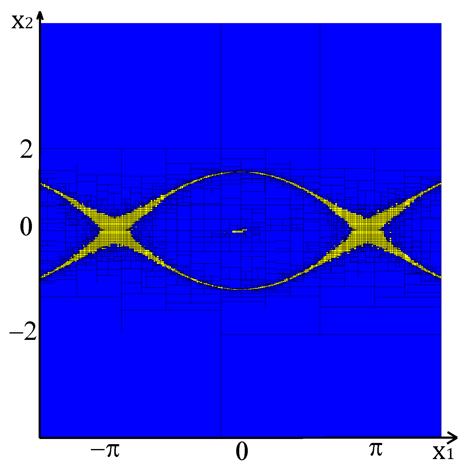
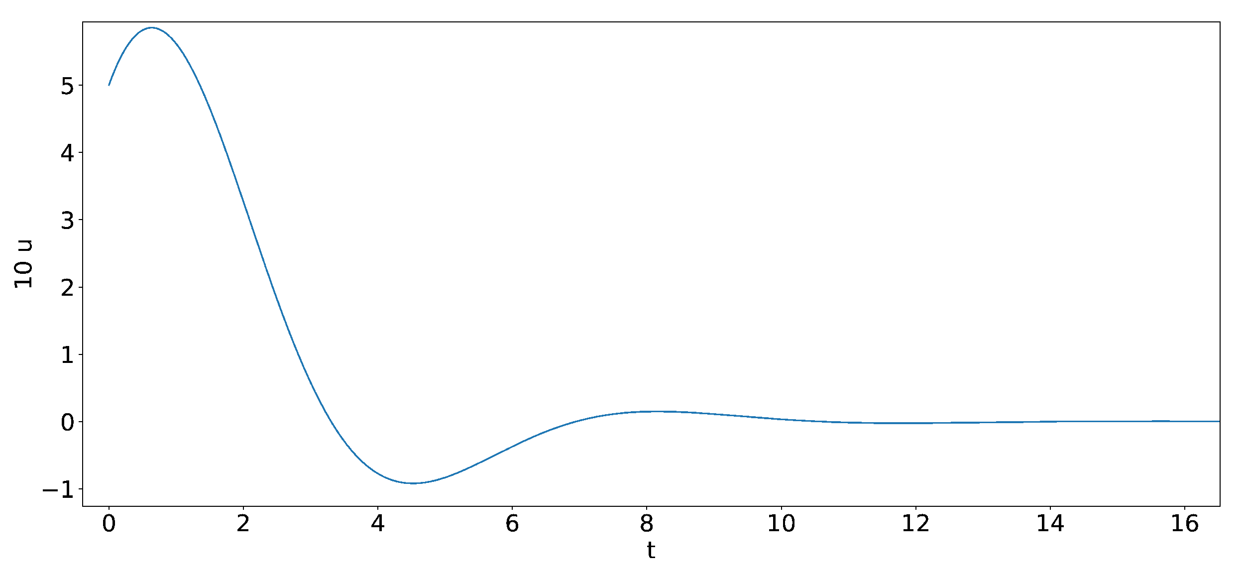
Under this preliminary consideration of the characteristics of invariant sets, states are not part of such sets if they are related to an inflection point in the form of a saddle point of the function
(see
Figure 1).
In fact, it suffices if any finite time derivative of
is not equal to zero for a point not belonging to the invariant set. This can also be confirmed when thinking of the Barbalat lemma, which states that, if a function has a finite limit for
, its uniformly continuous derivative will tend to zero [
40]. This can also be applied for the first derivative being the function and the second derivative being its first derivative, and so on:
Using the fact that the desired sliding surface itself and the first three derivatives of have to be zero as a necessary condition if holds constantly, the invariant limit set of the system can be found.
This statement can be verified by means of the following relations:
satisfied due to (
23)
satisfied due to (
23) ∧
= 0
satisfied due to (
23) and (
25).
Requiring furthermore that and hold, all further higher order derivatives of up to order seven are directly proven to be equal to zero.
Moreover, accounting for the fact that
holds by construction (see Equation (
7)), the relations (
23)–(
25) above turn into:
satisfied due to (
27)
satisfied due to (
27), where
in (
29) can be rewritten into:
Hence, the equivalent control designed in this paper guarantees that all temporal derivatives of
are perfectly equal to zero as soon as
has been reached. Enforcing furthermore that
(involved in (
23)–(
26)) holds after expressing these terms as functions of the controlled system dynamics on the invariant set during the interval based solution procedure in
Section 5 helps to improve the computational efficiency by means of defining so-called contractors that quickly shrink the search space for the invariant set towards the actual solution domain.
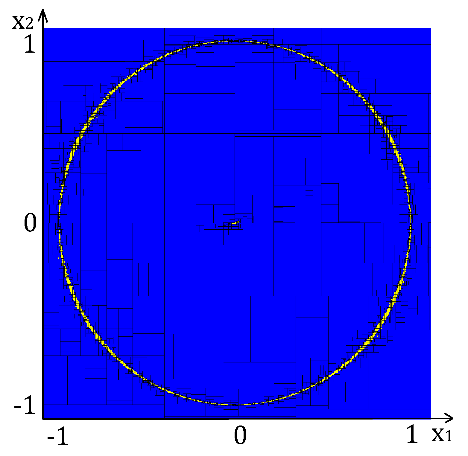
Remark 2. If an invariant set is computed according to the definition:it is not guaranteed that the system converges under all circumstances to the set:where the system is on the sliding surface. If the condition is not enforced explicitly in the interval based procedure described in the following section, the set may not only consist of the invariant set that is characterized by the sliding mode, but may also contain further fixed points. For example, for systems of dimension two, in which the examined sliding surface describes a closed trajectory in the state space in terms of a limit cycle, the Poincaré index theorem can be considered to visualize this fact. This theorem states that every limit cycle encloses at least one equilibrium point of the system, which will therefore also belong to the invariant set defined by [40]. 5. Interval Computation
The outer interval enclosure of the invariant set
of the controlled system in
, denoted exemplarily by
, is calculated using interval computation. This is possible due to the fact that the Lyapunov-like functions defined before provide inequalities. Therefore, it is checked for subintervals (i.e, boxes) covering the operating domain of interest if the conditions:
are satisfied in a domain that is a priori restricted to the set
. This last condition restricts the search space to a maximum admissible squared distance from the sliding surface.
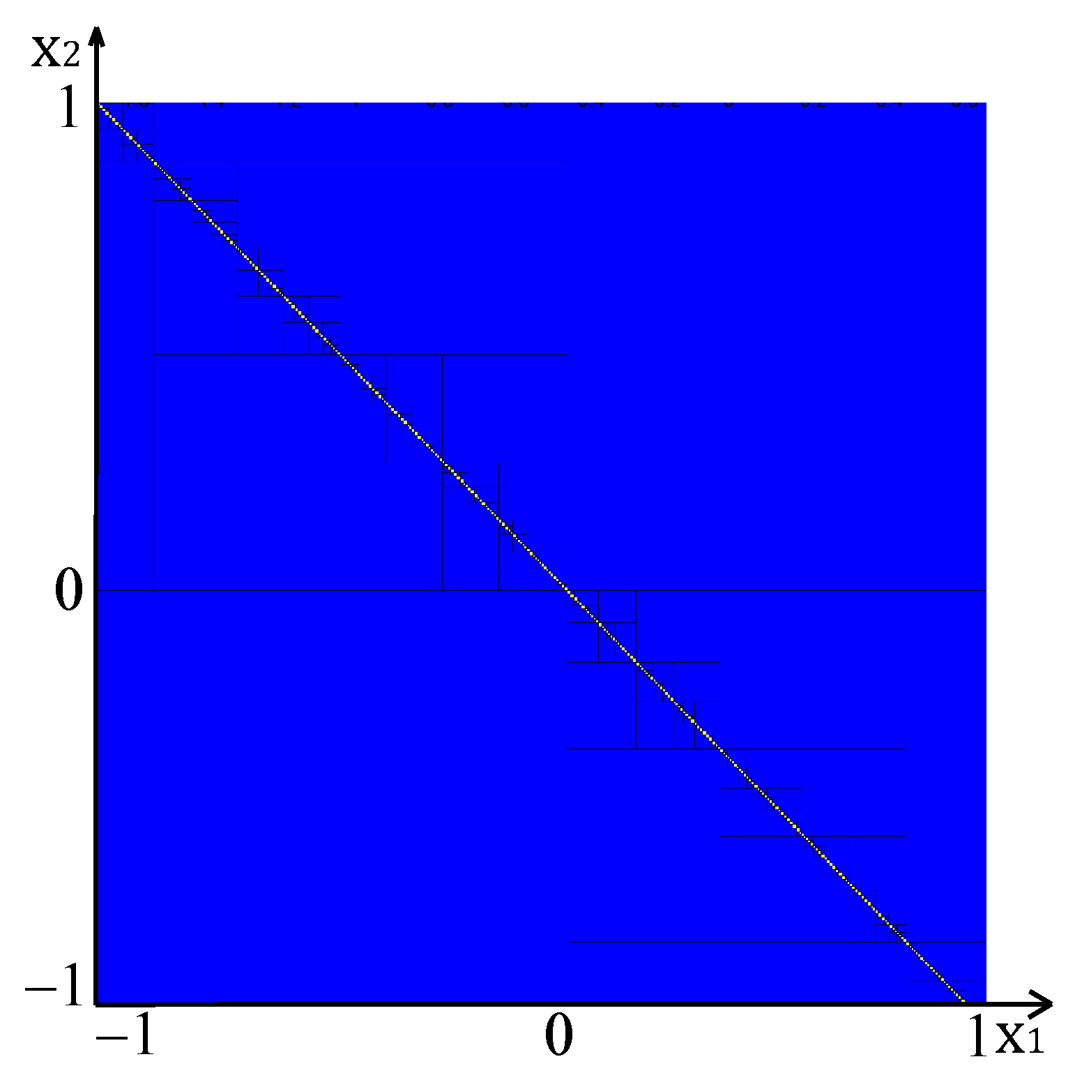
To solve a problem according to the specification (
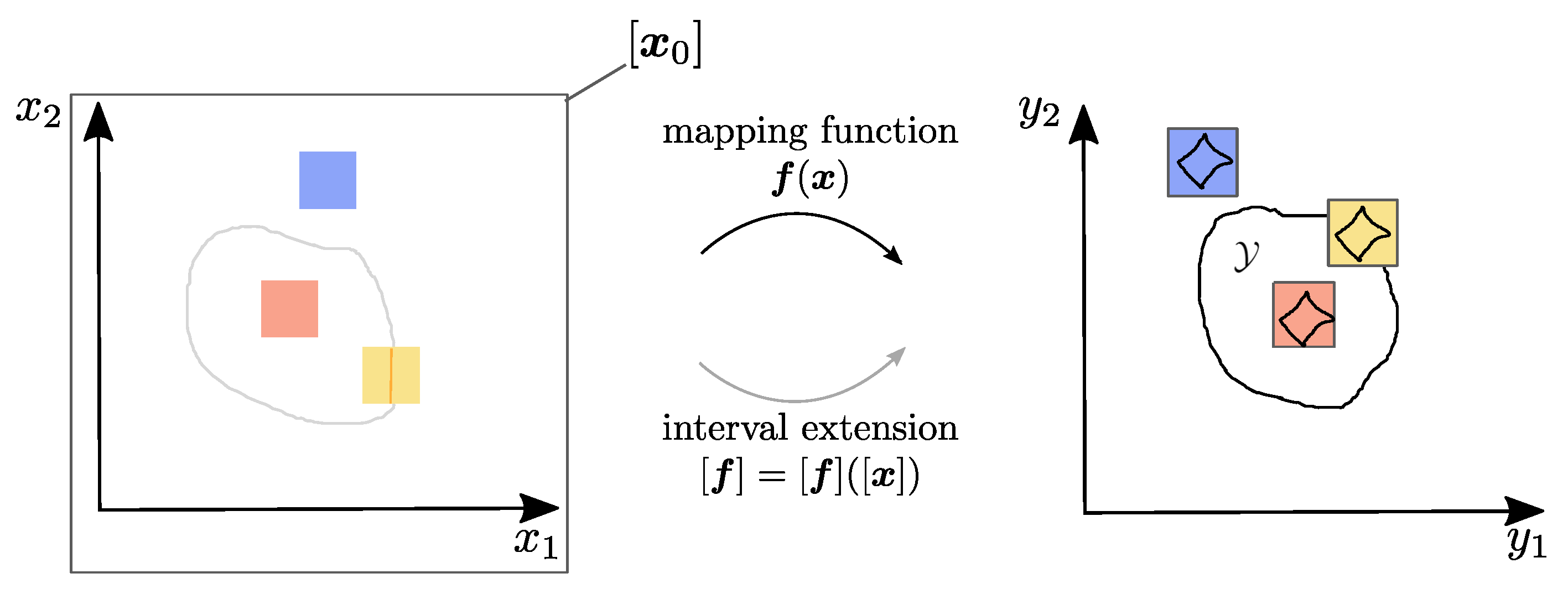
33), a general approach for interval techniques aiming at set inversion should be briefly described. The following description is based on
Figure 2. In the examined case, a set is known in the domain of
, and the set that should be found by the inversion technique is located in the
-plane. The function
performing the mapping,
, from the
-plane to the
-plane is assumed to be known together with a suitable inclusion function
that finds a rectangular box that encloses the set (gray). This function will not necessarily lead to the tightest enclosing box, but it is convergent with respect to interval bisections. The inverse mapping of
does not necessarily have to be known explicitly, so
either does not need to be or even cannot be determined analytically.
Starting with a sufficiently large box
in the
-plane that encloses the whole solution domain of interest, the corresponding box in
is calculated. It is then checked if it is located either outside the set (blue), inside the set (red), or if it is overlapping with both, the outer and interior domains, i.e., if the location is undecided (yellow). Whenever it is not sure if the box is inside or outside, the box in the
-plane will be split at the midpoint of each edge, and the procedure will be repeated for each of the new boxes. This is continued until a certain accuracy is reached. The red boxes will represent the corresponding set in the
-plane. This algorithm is called set inversion via interval analysis (SIVIA) [
2].
Note that interval computations are guaranteed in the following sense: If a box in the -plane has been found that is mapped into the interior of , it is guaranteed to be part of the true solution set , and vice versa, that if a box lies outside the solution set in the -plane, its counterpart in certainly contains no admissible solutions. If both cases are included in one box, it will, as mentioned before, either be split or, if the volume of the respective hypercuboid falls below some threshold value, be labeled as undecided.
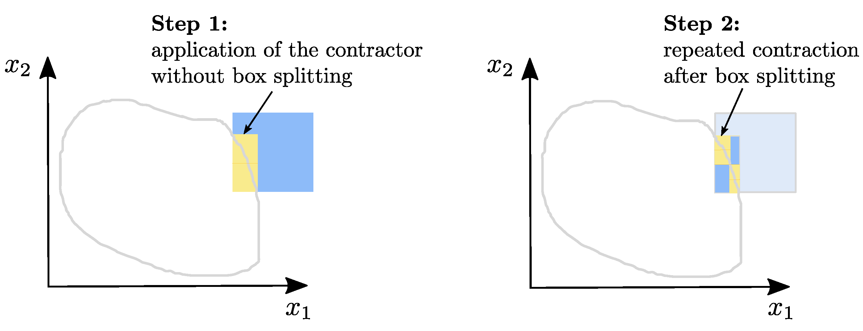
As this successive bisectioning scheme leads to lots of boxes that have to be checked ( boxes for a simultaneous subdivision of an n-dimensional box in each of its edges) the concept of contractors can effectively be applied to shrink a box as far as possible to the solution set. Here, the interval contraction is performed by means of each component of the vector valued function .
A contractor can be built by looking at the syntactic tree of the function
, which means a decomposition into primitive equations by defining auxiliary variables [
2]. In this way, the intervals can be contracted in a forward-backward manner. The forward part is where the definitions of the auxiliary variables are executed, and the backward part is where the original intervals are intersected with the newly calculated ones through the auxiliary variables’ definition.
This type of algorithm is described in more detail in [
2] and has been employed for an interval based parameter identification scheme in [
19]. Using this contractor, the first box will be blue, and inside this box, there will be a yellow one that is the smallest one to contain the whole solution set included in the first blue box, if the contractor is minimal. Then, the yellow box containing the solution set is split, and the procedure is repeated for each of the boxes. In this way, the boxes become smaller more quickly than in the case where every box is repeatedly divided.
Figure 3 illustrates this fact [
2].
To transfer this contractor approach to the problem defined in this paper according to Equation (
33), the following analogues are exploited: (i) the first condition
corresponds to
; (ii)
is generalized in terms of the
n-dimensional state vector; (iii) the value of zero is considered as the known set in the image space
. Analogously, contractors are also built for the further derivatives in (
33). All of these contractors are intersected with each other because all conditions should be satisfied simultaneously to provide an (outer) interval enclosure of the system’s invariant set.
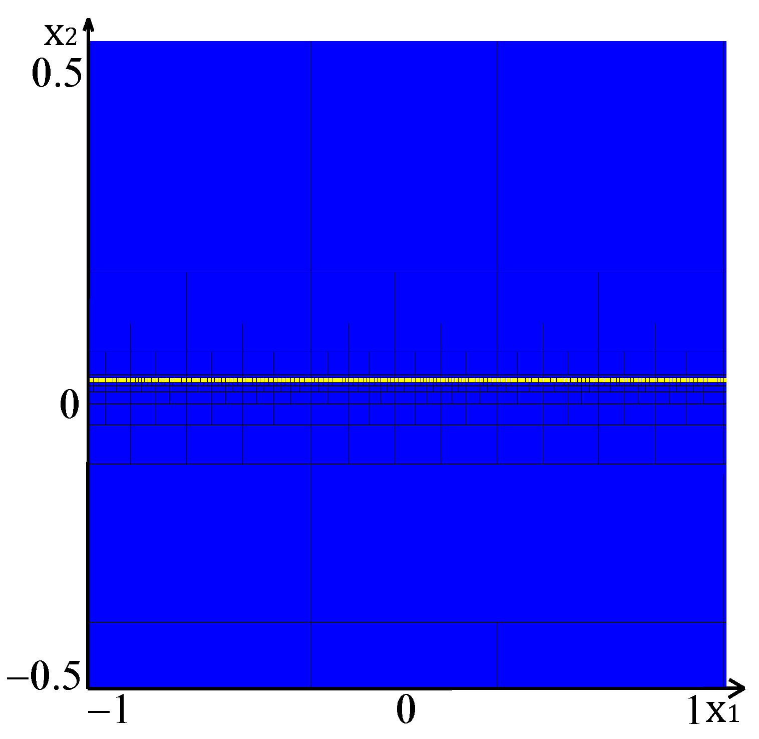
7. Conclusions and Outlook on Future Work
In this paper, a method to compute the invariant set of a nonlinear system controlled by sliding mode approaches, which were designed in such a way that structural singularities were guaranteed to be prevented, was suggested. Numerically, the invariant set could be obtained using interval computation, if the controller was designed according to the equation:
Avoiding singularities in u was ensured using a suitable Gröbner basis representation. The various investigated examples showed a surface represented by a closed curve, a case where Bézout’s identity had no solution and thus no controller can be found, and a surface that was a line. Additionally, a three-dimensional example was given and bounds, on the control input were considered.
The presented interval technique for the identification of invariant sets can easily be generalized towards the computation of the region of attraction of asymptotically stable equilibria of nonlinear feedback control systems by verifying those domains in the state space in which the time derivative
of a Lyapunov function candidate was strictly non-positive within a level set characterized by
, where this curve needed to be proven by the suggested approach not to coincide with an invariant set. Straightforwardly, also generalizations to the identification of domains in the state space, for which the stability of stochastic differential equations cannot be verified, became possible. Such domains were derived in [
48].
In future work, the suggested procedure for the computation of invariant sets can be extended by the consideration of set valued uncertainty in the state variables included in the control signal
, which result either from an imperfect state measurement or from uncertainty if the state information included in the feedback control law is reconstructed by means of an interval observer [
49]. Moreover, procedures for enhanced control parameterizations can be developed on the basis of the presented identification of invariant sets so that the volume of the intervals containing these sets is minimized. Hence, the aim will be to make the guaranteed provable stability domains as large as possible, as well as to maximize the regions of attraction of asymptotically stable equilibria by control re-parameterizations, to minimize the non-provable stability domains in the aforementioned stochastic settings, and to tune Lyapunov functions so that the provable stability domains show a minimum amount of pessimism.


