The Research of Improved Active Disturbance Rejection Control Algorithm for Particleboard Glue System Based on Neural Network State Observer

Abstract

For achieving high-performance control for a particleboard glue mixing and dosing control system, which is a time-delay system in low frequency working conditions, an improved active disturbance rejection controller is proposed. In order to reduce overshoot caused by a given large change between the actual output and expected value of the control object, a tracking differentiator (TD) is used to arrange the appropriate excesses. Through the first-order approximation of the time-delay link, the time-delay system is transformed into an output feedback problem with unknown function. Using the neural network state observer (NNSO), a sliding mode control law is used to achieve the accurate and fast tracking of the output signal. Finally, the numerical simulation results verify the effectiveness and feasibility of the proposed method.

1. Introduction

In recent years, the use of alternative wood resources in the particleboard industry has increased, mainly because of the declining potential of forests [1]. Rational use of non-wood raw materials instead of wood to produce particleboard can improve the utilization rate of forest resources and protect the ecological environment.

In the production process of particleboard mixing and dosing, the glue is an important link. The amount of glue directly affects the quality of finished particleboard products; when there is too much glue the produced particleboard will have high moisture content, which leads to foaming and reduces production; when the amount of glue is too little, the plasticity of particleboard will decrease, and then the product quality will decline. In the low frequency working conditions of particleboard production, the hysteresis and inertia of the motor and pump will greatly affect the control effect of the system. Therefore, accurate glue flow control is a problem worth studying.

Since the emergence of proportional–integral–derivative (PID) control technology, a large number of engineering problems have been solved [2,3]. Because of the advantages of simple structure and high reliability, it still has an overwhelming advantage in engineering applications today and the production of particleboard is one of them. There are many improvement methods for PID, which are widely used and have good practical effects. The fractional order control system has attracted the attention of many scholars [4,5,6], and some of them have applied it to PID control to enhance the control effect [5,6,7,8,9]. Reference [7] utilized a fractional order controller to eliminate steady state error and enhance the robustness toward plant gain variations and also good disturbance rejection. However, the main problem is that the passive way to eliminate errors based on error feedback lags behind the disturbance effect, and may cause system oscillation or serious overshoot because of the excessive initial control. In order to prevent such situations in particleboard glue mixing and dosing, the traditional PID control technology still needs to be further improved.

Active disturbance rejection control (ADRC) is proposed by Han and has been widely used in Reference [10,11,12,13]. Tracking differentiator (TD), as a part of it, solves the above problems well. TD has the function of resisting random noise [14] and can deal with the differential tracking problem of non-differentiable functions in the classical sense. After the output of the differentiator is obtained, the fastest synthesis function is designed to arrange the transition process of the closed-loop system.

The stability of the controlled system has always been the goal of scholars. Though feedforward control can effectively suppress specific disturbances in time, the premise is that the disturbance and the system structure are known. In the actual production process, the exact model of the system is difficult to obtain, so the feedforward disturbance rejection effect is not obvious in the complex disturbance environment. In order to not only solve the problem of model uncertainty, but also solve the problem of external disturbance of the system, the state observer has been studied by scholars in recent years [15,16,17,18,19]. Reference [15] proposed a compound controller based on multiple-input and multiple-output extended-state-observer to solve the difficulties associated with the unmeasured velocities, unknown disturbances, and uncertain hydrodynamics of the robot. Peng presented a design method for under-actuated autonomous underwater vehicles, where an extended state observer is developed to recover the unmeasured velocities as well as to estimate total uncertainty induced by internal model uncertainty and external disturbance in Reference [16]. Reference [17] studied a novel predictor-based extended state observer for each follower with relative output information of the neighboring agents for multiagent systems. In view of this, ADRC regards state observer technology as its core part so that ADRC can simplify the controlled system into a set of disturbed systems including external disturbance input, internal disturbance, uncertainty, and un-modeled parts of the system model, which will be seen as all disturbance and estimated by the observer.

Although this observer can estimate the disturbance for the controller and reduce its influence on the control effect, it can no longer meet the requirements of scholars for the control accuracy with the progress of technology [20,21]. Artificial neural networks are mathematical models that mimic the structure and function of brain neural networks. Because of its powerful learning ability and adaptability, neural networks are very suitable for approximating unknown functions. This has been widely applied by scholars to the approximation of unknown uncertainties in linear or nonlinear control systems [22,23].

Based on the arrangement of the TD and conversion process, the error signal can be tracked after the conversion process. Using this signal and its differential signal, it can be controlled by nonlinear states error feed-back (NLSEF) in Reference [24]. However, the traditional control rate does not have good control effects on system uncertainty, disturbance, and unmolded dynamics. Even if the neural network state observer (NNSO) is used to compensate for all the uncertainties of the system, it has certain modeling uncertainty which needs to be improved.

For the above problem, some scholars have found that sliding mode control (SMC) can solve it well [25,26,27]. As an alternative to the typical robust control scheme, SMC is a typical control method. The advantage of SMC is that it can overcome the uncertainty of the system and has strong robustness to disturbance and un-modeled dynamics, especially for the control of nonlinear systems. Some scholars have studied the comparison of SMC and ADRC [28]. Reference [28] concerned with the boundary feedback stabilization of a one-dimensional Euler–Bernoulli beam equation with the external disturbance flowing to the control end, it is shown that the external disturbance can be attenuated in the sense that the resulting closed-loop system under the extended state feedback tends to any arbitrary given vicinity of zero as the time goes to infinity. The advantage of SMC is that it can overcome the uncertainty of the system, and has strong robustness to interference and unmolded dynamics. This can make up for the uncertainty of NNSO itself.

Although the stability of the system can be improved through the above analysis, due to the controlled plant, the particleboard glue mixing and dosing system is a time-delay system in low frequency working conditions (15 HZ input frequency), and it is often difficult to achieve satisfactory results. The time delay will bring additional phase lag, and the phase lag will increase with the increase of frequency. To solve the problem of time-delay, a first-order approximation for the dead time is used in Reference [29]. In this way, further precise control can be achieved under the low frequency conditions of the glue application.

Considering that ADRC theory has not been applied in particleboard production, we propose an improved active disturbance rejection controller for the particleboard glue mixing and dosing system in this paper. The main contributions of this paper are summarized as follows:

(1)

The process of mixing and dosing the glue for particleboard is introduced and so is the composition of the system. Then we establish the state space equation.

(2)

We construct an improved controller using ADRC approach. The improved NNSO is utilized to observe disturbance for control compensation and estimate the system state variables. To simplify the controller, the improved TD is used to achieve smooth transmission of differential signals and realize optimal configuration of closed-loop system transition processes. The SMC is introduced to improve the robustness for the disturbance not observed by NNSO.

The paper is organized as follows: Section 2 introduces the particleboard glue mixing and dosing system. In Section 3, an improved ADRC strategy based on sliding mode control is proposed and proves the asymptotic stability of the proposed control strategy and observer convergence by Lyapunov analysis. In Section 4, simulation results are shown to verify the effectiveness of the proposed control method. The conclusion of the paper is shown in Section 5.

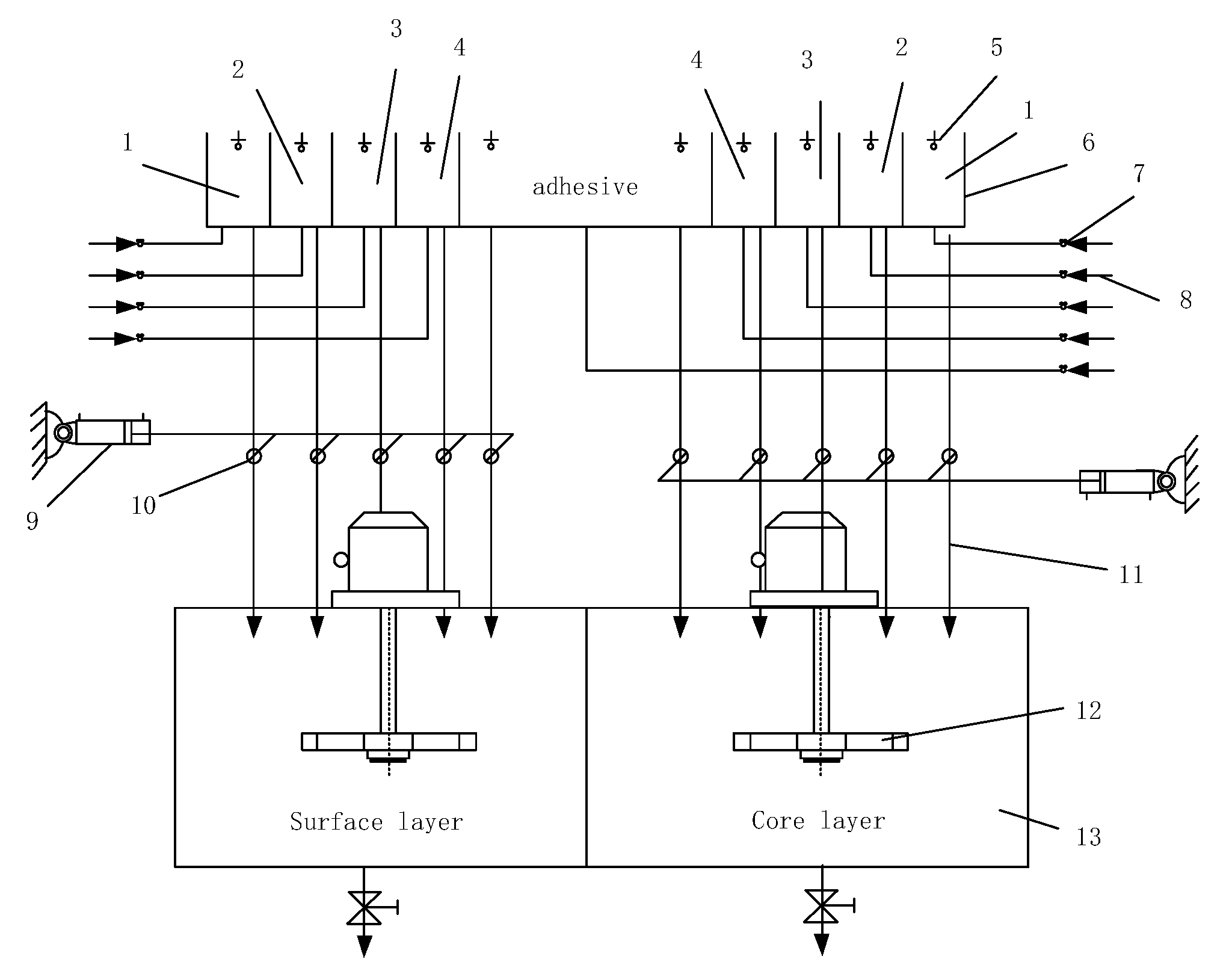
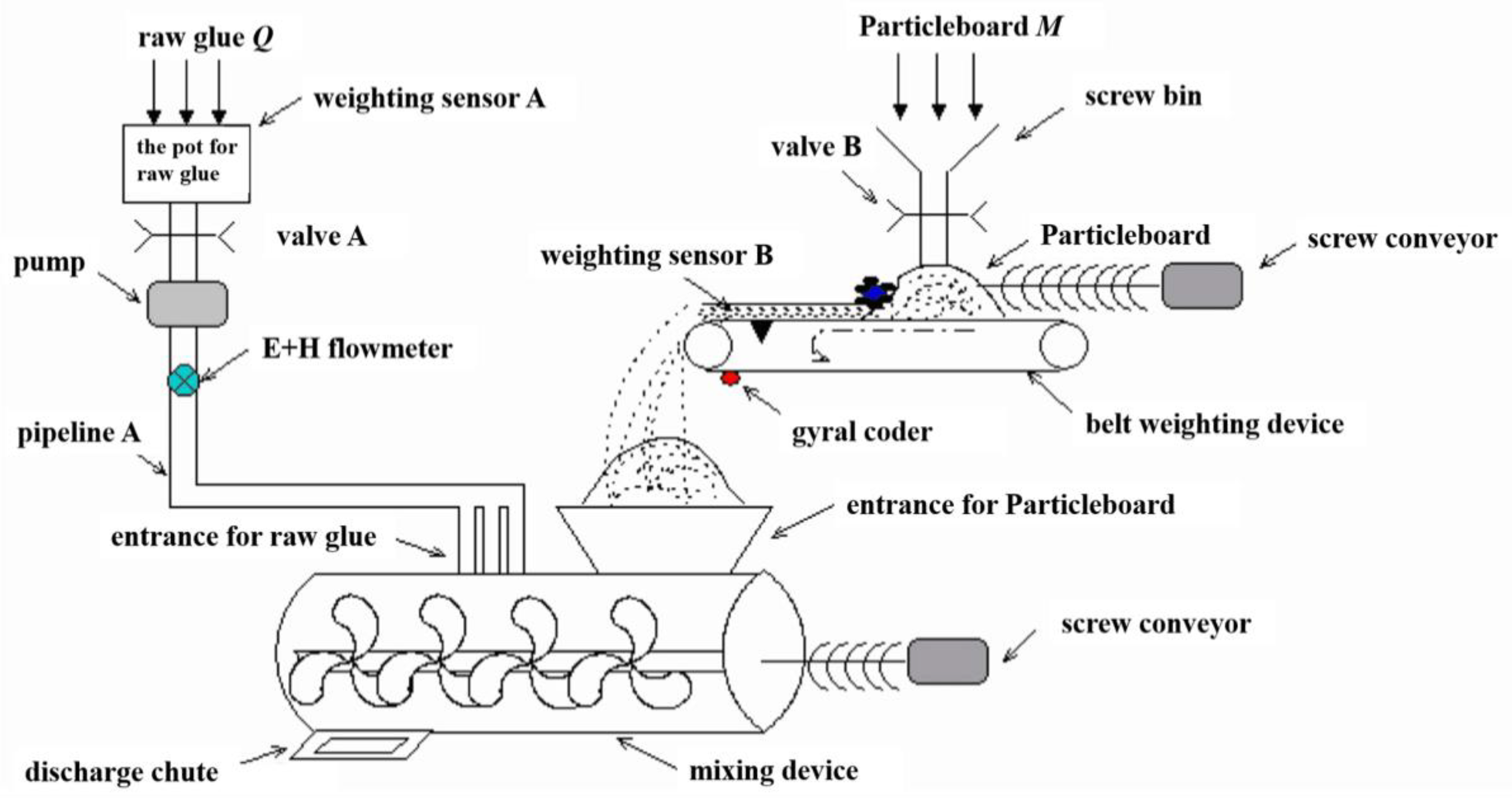
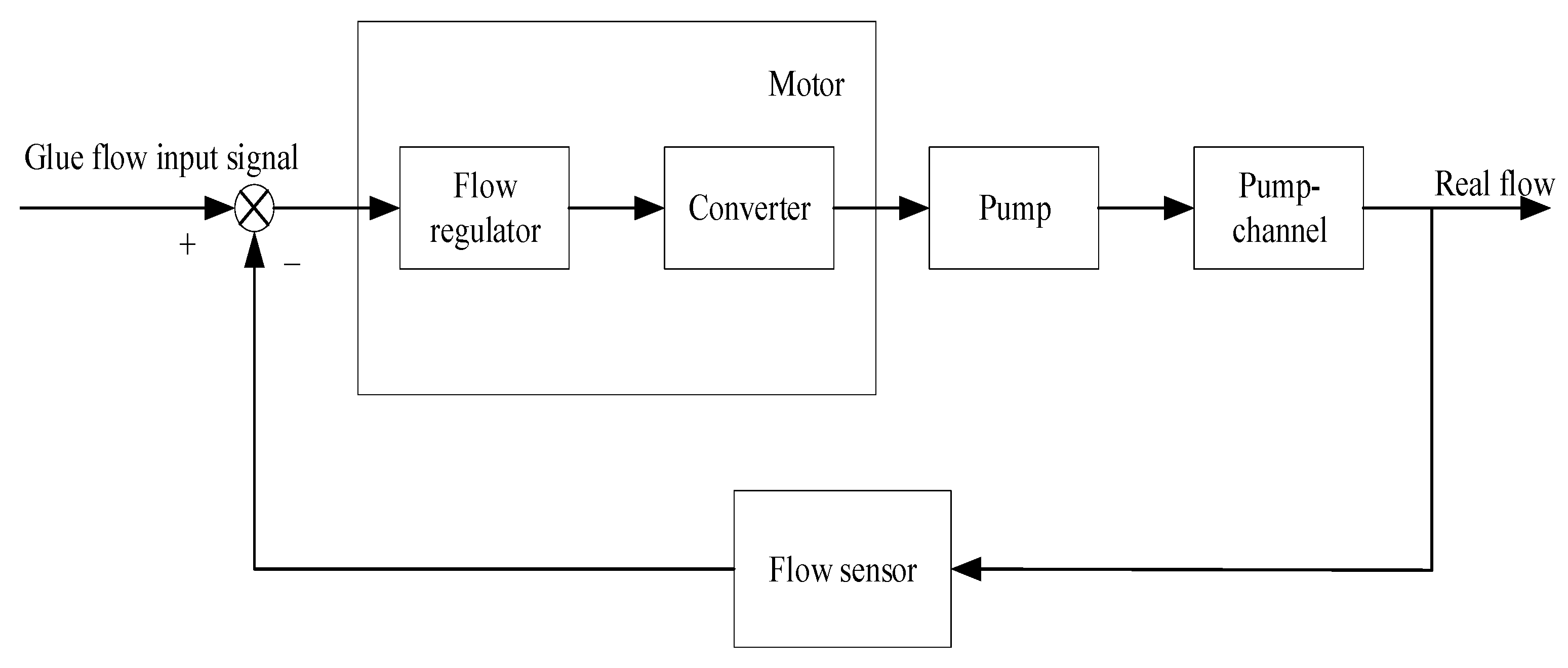
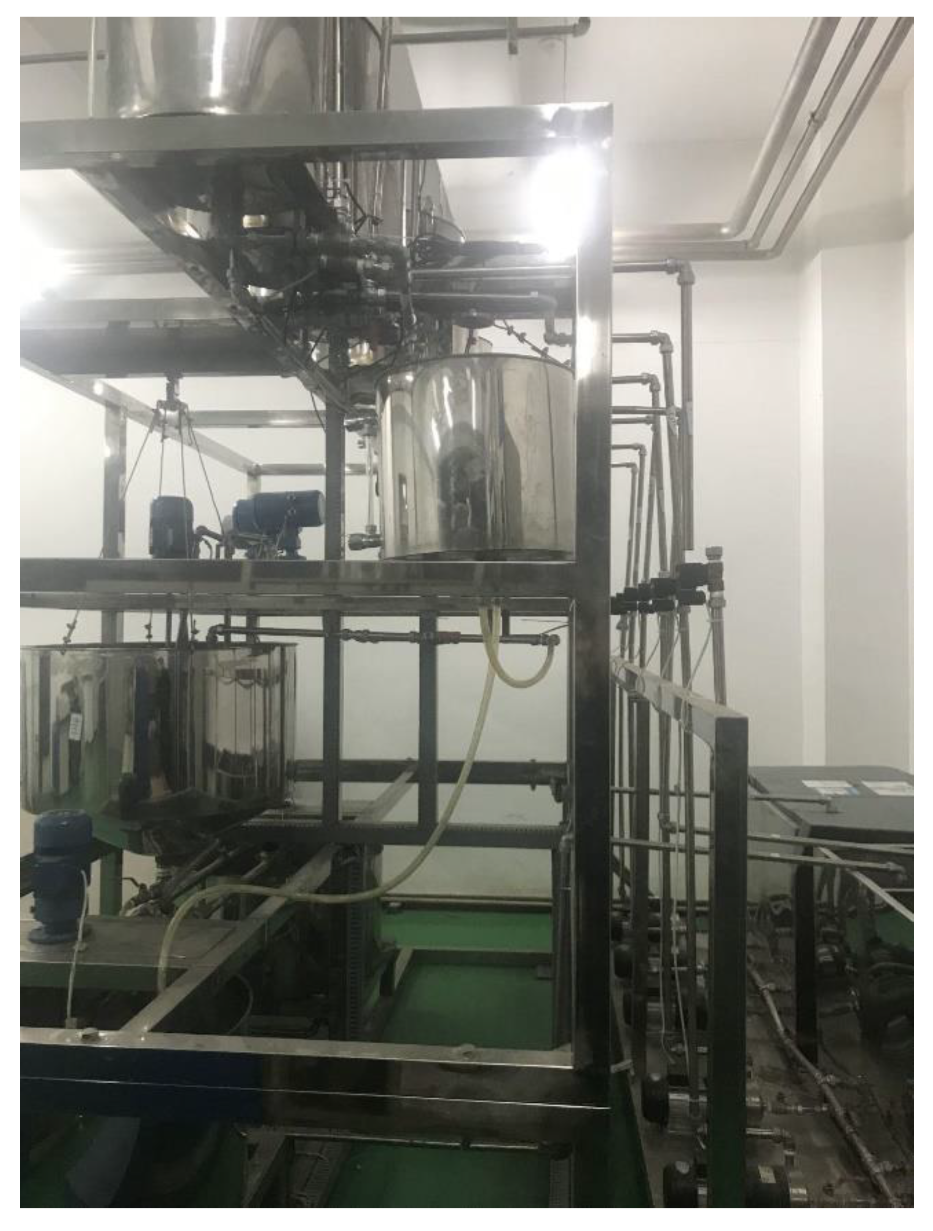
2. Process and System Description

The bonding force between particleboards is obtained by the bonding of adhesives, and the specific surface area of particles is large, so uniform sizing is very important. Particleboard bonding adhesives belong to thermosetting adhesives, which need heating to achieve curing bonding and the curing process is irreversible. Therefore, in the process of sizing, the control system must ensure that there is no overshoot.

The system is divided into two parts: glue mixing and glue dosing. The schematic diagram of glue mixing system is shown as Figure 1. The volume of various raw materials, include curing agent, waterproof agent, curing buffer agent, water, and adhesive, is measured by a liquid level detector. The electronic control throttle valve, that controls itself, is set to the proportion for the system in advance. When the required material reaches the expected value, the valve will close itself. Then the raw materials are mixed by gravity flow into the mixing tank. Ball valves are used to control the amount of raw materials required. According to the formula entered into the system in advance, it controls the switch by itself to the amount of raw materials transferred to the glue mixing case, and all the materials are mixed by the agitator in the case. The glue mixing case is divided into two parts, one for the surface layer of the particleboard and the other for the core layer.

The sketch of the controlled system is shown in Figure 2. It consists of a particleboard supported device, a glue supported device, and a mixing device. The conveyor chute and the belt weighing device make up the supported device and all particleboards are supported by it. The screw conveyor feeds the particleboard into the discharge chute; the weighing sensor measures the weight of the particleboard; and the rotation speed of the belt weighing device is measured by gyral coder. The glue supported device consists of a glue control pump and a flowmeter, which the E+H type flowmeter is chosen. The glue and particleboard are mixed by a mixing device.

During the process of dosing particleboard, the screw conveyor conveys the particleboard to the mixing device and through the screw bin and valve B. The instantaneous weighing signal is gathered by weighing sensor B, which is located on the weighing conveyor belt. When the particleboards are transported, the instantaneous weight of the glue is calculated on the basis of the amount of the glue input. Then, in the light of the relationship between the rotation speed and the output of the pump, we calculate the pump speed.

The essential structure of the particleboard mixing and dosing system is shown in Figure 3. Glue flow input signal is the desired value of the controller. The ultimate goal of the control system is to ensure that the output glue flow reaches the desired value. Firstly, we get the glue flow through the flow sensor. The sensor is an E+H flowmeter as shown in Figure 2. It measures the output glue flow velocity in the pipe and the input value is compared with it and the obtained error is sent to the controller. For minimizing the error, the controller continuously tinkers with the frequency of the converter and, through it, the speed of the squirrel-cage motor is changed and it will result in the change of the output glue flow. By doing this, the controlled glue supplying pump can be stable.

Under low frequency (15 HZ input frequency) conditions during particleboard dosing and mixing, the controlled system becomes a time-delay system due to the hysteresis and inertia of the motor and pump. A time-delayed object can be formalized as a transfer function mathematical model as follows.

$$G_P(s)=G_0(s)e^{-\tau s}=\frac{b}{s^n+a_{n-1}{s}^{n-1}+\cdots a_{1}s+a_0}{e}^{-\tau s},$$

(1)

where $\tau$ is the pure lag time constant, $G_0(s)$ represents the part of the object that does not include the lag link, $b$, $a_0$, $a_1$$\cdots$$a_{n-1}$ are object parameters.

For industrial objects with time lag, Equation (1) can be simplified as a first-order inertial link or a second-order oscillating link and described as a first-order time-delay system (FOPTD) or a second-order time-delay system (SOPTD), which is represented by Equations (2) and (3) respectively.

$$G_{POPTD}(s)=\frac{b}{s+a}{e}^{-\tau s},$$

(2)

$$G_{SOPTD}(s)=\frac{b}{s^2+a_{1}s+a_0}{e}^{-\tau s},$$

(3)

Most of the time, all the poles of the system are stable when $a>0$, $a_0>0$, $a_1>0$. When $a>0$ or $a_0=0$ Equations (2) and (3) become pure integrator with a time-delay link and it is intractable for controlled system. Furthermore, the control problem of the system will be more challenging if $a<0$ or $a_0<0$, $a_1<0$ due to the unstable poles.

We choose the controlled objects as shown in Equation (4)

$$G_{SOPTD}(s)=\frac{0.01578}{s^2+0.276s+0.01578}{e}^{-3.73s}$$

(4)

When the time delay $e^{-3.73s}$ is approximately the first order inertial link $\frac{1}{3.73s+1}$, the controlled object shown in Equation (4) becomes

$$G_0(s)=\frac{0.01578}{s^2+0.276s+0.01578}\cdot \frac{1}{3.73s+1}$$

(5)

In order to facilitate the controller design, we transform the representation of the system from frequency domain to time domain for analysis. Considering the disturbance that the system will suffer and the system uncertainty, the state space equation is shown in Equation (5)

$$\{\begin{array}{c}{\dot{x}}_1=x_2\hfill \\ {\dot{x}}_2=x_3\hfill \\ {\dot{x}}_3=a\left(x_1,x_2,x_3\right)+bu+f\left(x_1,x_2,x_3,w(t),t\right)\hfill \\ y=x_1\hfill \end{array},$$

(6)

where $a\left(x_1,x_2,x_3\right)=-0.544x_3-0.09x_2-0.004x_1$, $b=0.004$, $f\left(x_1,x_2,x_3,w(t),t\right)=w(t)+\mathsf{\Delta }a\left(x\right)$ represents the total disturbance of the system, where $w\left(t\right)$ represents the disturbance, $\mathsf{\Delta }a\left(x\right)$ represents the model uncertainty.

3. Design of the Compound Controller

In this section, we designed an improved ADRC controller for particleboard glue mixing and dosing system with the low frequency condition. An improved ADRC strategy was designed. Firstly, the TD was designed to eliminate the noise of the acquired desired signal and track it fast. Secondly, the NNSO was utilized to estimate the total disturbance and compensate the system model with the estimation. Finally, the improved sliding mode control law was designed instead of NSLEF to improve system robustness.

3.1. Designs of the Tracking Differentiator

The TD in traditional ADRC is usually discrete as shown in Equation (7):

$$\{\begin{array}{c}{x}_1(k+1)=x_1(k)+h{x}_2(k)\hfill \\ x_2(k+1)=x_2(k)+h\left\{-r^2\left[x_1(k)-y_d(k)\right]-2r{x}_2(k)\right\}\hfill \end{array},$$

(7)

where $y_d$ is input signal, $x_1$ is the transition process of input signal, and $x_2$ is its differential signal. $h$ is an integral step that is designed to set the corresponding step size according to the engineering requirements and the controller capability, $r$ is the adjustable speed factor that adjusts the speed of excessive processing according to the actual process needs. Thus, we introduce a continuous form of TD as shown in Equation (8).

$$\{\begin{array}{c}{\dot{x}}_1=x_2\hfill \\ {\dot{x}}_2=-rsign\left[x_1-y_d(t)+\frac{x_2\left|x_2\right|}{2r}\right]\hfill \end{array},$$

(8)

The function of TD is shown in Figure 4. When the input signal of the system has internal disturbance noise or change uncertainties, TD provides the transition process through the input signal to realize the smooth processing of the signal, thus ensuring the continuity of the input of the controller and reducing the negative impact of the disturbance.

As Figure 4 shows we can get a smoother curve for the square wave signal with noise interference after TD, and differential signals are also obtained which can be transmitted to the controller for control.

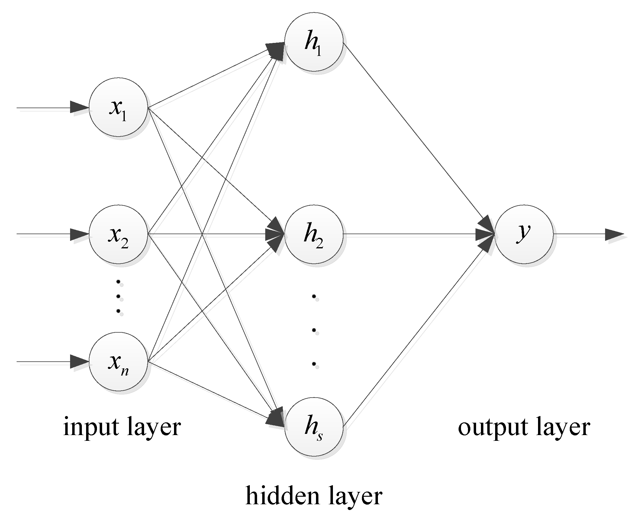
3.2. Neural Network Extend State Observer

3.2.1. Designs of Neural Network State Observer

Then the NNSO is designed for the new system:

$$\dot{\hat{X}}=A\hat{X}\left(t\right)+BU\left(t\right)+f\left(\hat{X}\left(t\right)\right)+L\left(Y\left(t\right)-C\hat{X}\left(t\right)\right),$$

(9)

where $L\in R$ is observer gain matrix, $\hat{X}\left(t\right)$ is state observation, $f\left(\hat{X}\left(t\right)\right)$ is total disturbance observation, and the state error is defined as:

$$\tilde{X}\left(t\right)=X\left(t\right)-\hat{X}\left(t\right),$$

(10)

and we can get the error dynamic equation of observer state as follows

$$\dot{\tilde{X}}=\left(A-LC\right)\tilde{X}\left(t\right)+f\left(\tilde{X}\left(t\right)\right),$$

(11)

where $f\left(\tilde{X}\left(t\right)\right)=f\left(X\left(t\right)\right)-f\left(\hat{X}\left(t\right)\right)$. Let $L={\left[L_1,L_2,\cdots ,L_n\right]}^T$ satisfy $A-LC$ Hurwitz condition and $L_i={\beta }_i/{\epsilon }^i$, where $\epsilon >0$. Equation (12) is an error dynamic equation and can be regarded as a constant coefficient differential equation with input $f\left(\tilde{X}\left(t\right)\right)$ to describe a linear system. The solution of this equation is

$$\dot{\tilde{X}}=e^{\left(A-LC\right)t}\tilde{X}\left(0\right)+{\displaystyle {\int }_0^t{e}^{e^{\left(A-LC\right)\left(t-\tau \right)}}f\left(\tilde{X}\left(\tau \right)\right)}d\tau ,$$

(12)

The basic idea of NNSO is to use the input and output of the system to observe all states including the original state variables and disturbances of the system. The core of the ADRC control strategy is to estimate $f\left(X\left(t\right)\right)$ and eliminate it. Since the radial basis function (RBF) neural network can approach the nonlinear function with accuracy, we introduce the neural network to approach $f\left(X\left(t\right)\right)$, so that NNSO can accurately observe the total disturbance in the system. The block diagram of the neural network is shown in Figure 5.

Therefore, a three-layer RBF neural network is used to approach the interference. The first layer is the input layer of $n$ neural networks with fixed weight. The second layer is the hidden layer of $s$ neural networks with a weight of $\left\{w_{ij},i=1,2,\cdots ,n,j=1,2,\cdots ,s\right\}$. The third layer is the output layer, a linear combination of the output of each neural network. The input-to-output mapping represented by the RBF neural network is

$$f\left(X\left(t\right)\right)={\displaystyle \sum _{j=1}^s{w}_{ij}{\sigma }_j}\left(\Vert x-c_j\Vert ,{\rho }_j\right),\hspace{1em}i=1,2,\cdots ,n,$$

(13)

where $X\in R^n$ is the network input vector, the activation function is an $\sigma (·)$ Gaussian function for which the center is $\left\{c_j,\hspace{1em}j=1,2,\cdots ,s\right\}$ and the width is $\left\{{\rho }_j,\hspace{1em}j=1,2,\cdots ,s\right\}$. The upper bound of the ideal weight $W^T$ of the output layer is ${\Vert W\Vert }_F\le W_M$. When the output approximates the disturbance, it can be expressed as

$$f\left(X\left(t\right)\right)=W^T\sigma \left(X\right),$$

(14)

The real ideal weight is ${\hat{W}}^T\sigma \left(\hat{X}\right)$ after the neural network learning training, so the observation of $f\left(X\left(t\right)\right)$ is

$$f\left(\hat{X}\left(t\right)\right)={\hat{W}}^T\sigma \left(\hat{X}\right),$$

(15)

where $\Vert \sigma \left(\hat{X}\right)\Vert \le {\sigma }_M$, the neural network approximation error is

$$\begin{array}{cc}\hfill f\left(\tilde{X}\left(t\right)\right)& =W^T\sigma \left(X\right)-{\hat{W}}^T\sigma \left(\hat{X}\right)\hfill \\ & =W^T\sigma \left(X\right)-{\hat{W}}^T\sigma \left(\hat{X}\right)+W^T\sigma \left(\hat{X}\right)-W^T\sigma \left(\hat{X}\right)\hfill \\ & ={\tilde{W}}^T\sigma \left(X\right)+\omega \left(t\right)\hfill \end{array},$$

(16)

where $\omega \left(t\right)=W^T\left(\sigma \left(X\right)-\sigma \left(\hat{X}\right)\right)$ is bounded approximation error, which satisfies $\Vert \omega \left(t\right)\Vert \le \overline{\omega }$

Considering Equations (10) and (16), we get the observer

$$\dot{\hat{X}}=A\hat{X}\left(t\right)+BU\left(t\right)+{\hat{W}}^T\sigma \left(\hat{X}\right)+L\left(Y\left(t\right)-C\hat{X}\left(t\right)\right),$$

(17)

$$\hat{Y}\left(t\right)=C\hat{X}\left(t\right),$$

(18)

and the error dynamic equation of observer state is

$$\dot{\tilde{X}}\left(t\right)=\left(A-LC\right)\tilde{X}\left(t\right)+{\tilde{W}}^T\sigma \left(\hat{X}\right)+\omega \left(t\right),$$

(19)

$$\tilde{Y}\left(t\right)=C\tilde{X}\left(t\right),$$

(20)

Using the gradient descent calculation method, we define the network learning objective function as

$$J=\frac{1}{2}{\tilde{Y}}^T\tilde{Y},$$

(21)

and the network learn equation is

$$\dot{\hat{W}}=-\eta \left(\frac{\partial J}{\partial \hat{W}}\right)-\kappa \Vert \tilde{Y}\Vert \hat{W},$$

(22)

where $\kappa >0$, $\eta >0$ is the learning rate of neural network. Differentiating Equation (22) gives

$$\frac{\partial J}{\partial \hat{W}}=\frac{\partial J}{\partial \tilde{Y}}\frac{\partial \tilde{Y}}{\partial \tilde{X}}\frac{\partial \tilde{X}}{\partial \hat{W}}=-{\tilde{Y}}^{T}C\frac{\partial \tilde{X}}{\partial \hat{W}},$$

(23)

In order to simplify the training algorithm and avoid complex gradient calculation, let $\dot{\hat{X}}\left(t\right)=0$, invoking Equation (20)

$$\frac{\partial \tilde{X}}{\partial \hat{W}}\approx {\left(A-LC\right)}^{-1}\frac{\partial \tilde{X}}{\partial \hat{W}},$$

(24)

Considering Equations (16), (24) and (25), we get the adaptive law

$$\dot{\hat{W}}=-\eta {\left({\tilde{X}}^T{C}^{T}C{\left(A-LC\right)}^{-1}\right)}^T\sigma \left(\hat{X}\right)-\kappa \Vert C\tilde{X}\Vert \hat{W},$$

(25)

3.2.2. Stability Analysis of Neural Network Extend State Observer

For the convenience of the following analysis, the two following lemmas are given:

Lemma 1 [30].

Given a matrix$A=\left[a_{ij}\right]$, the Frobenius norm is defined as the root of the sum of the squares of all elements

$${\Vert A\Vert }_F^2\equiv {\displaystyle \sum a_{ij}^2=tr(A^{T}A)},$$

(26)

it is compatible with the vector 2-norm in that

$${\Vert Ax\Vert }_2\le {\Vert A\Vert }_F{\Vert x\Vert }_2,$$

Lemma 2 [31].

A mapping$H:L_{p,c}\to L_{p,e}$is said to be stable if there exist positive numbers$\gamma$and$\xi$such that$\Vert {\left(Hu\right)}_l\Vert \le \xi +\gamma {\Vert u_t\Vert }_p$for all$u\in L_{p,e}$and all$t\in \left[0,+\infty \right)$.

Theorem 3.1.

The state estimation error approaches zero asymptotically ($\underset{t\to \infty }{\lim }\tilde{X}=0$), provided

1. 

$\gamma <{\lambda }_{\min }\left(Q\right)/2{\lambda }_{\max }\left(P\right)$, where$P$,$Q$are positive definite symmetric matrices and${\lambda }_{\min }$and${\lambda }_{\max }$represent the minimum eigenvalue and the maximum eigenvalue of the matrix respectively,

2. 

the Lyapunov function${\left(A-LC\right)}^{T}P+P\left(A-LC\right)=-Q$holds.

Proof. 

Choose the Lyapunov function for the observer as

$$V_o=\frac{1}{2}{\tilde{X}}^{T}P\tilde{X}+\frac{1}{2}tr\left({\tilde{W}}^T{\kappa }^{-1}\tilde{W}\right),$$

(27)

Differentiate Equation (28) and we get

$$\begin{array}{cc}\hfill {\dot{V}}_o& =\frac{1}{2}{\dot{\tilde{X}}}^{T}P\tilde{X}+\frac{1}{2}{\tilde{X}}^{T}P\dot{\tilde{X}}+tr\left(\dot{\tilde{W}}{\kappa }^{-1}\tilde{W}\right)\hfill \\ & =\frac{1}{2}{\tilde{X}}^{T}Q\tilde{X}+{\tilde{X}}^{T}P\left[{\tilde{X}}^{T}P\tilde{W}\sigma \left(\hat{X}\right)+\omega \left(t\right)\right]\hfill \\ & +tr\left[{\tilde{W}}^{T}R\tilde{X}{\sigma }^T\left(\hat{X}\right)+{\tilde{W}}^T\Vert C\tilde{X}\Vert \left(W-\tilde{W}\right)\right]\hfill \\ & \le -\frac{1}{2}\Vert \tilde{X}\Vert {\lambda }_{\min }\left(Q\right)\Vert \tilde{X}\Vert +\Vert \tilde{X}\Vert \cdot \Vert P\Vert \left(\Vert \tilde{W}\Vert {\sigma }_M+\overline{\omega }\right)\hfill \\ & +{\sigma }_M\Vert \tilde{W}\Vert \cdot \Vert R\Vert \cdot \Vert \tilde{X}\Vert +\left(W_M\Vert \tilde{W}\Vert -{\Vert \tilde{W}\Vert }^2\right)\Vert C\Vert \cdot \Vert \tilde{X}\Vert \hfill \end{array},$$

(28)

According Equation (29), when ${\dot{V}}_o\le 0$ the inequality holds

$$\Vert \tilde{X}\Vert \ge \left(2\Vert P\Vert \overline{\omega }\right)+\left({\sigma }_M\Vert P\Vert +W_M\Vert C\Vert +{\sigma }_M{\Vert R\Vert }^2/2\right)/{\lambda }_{\min }\left(Q\right),$$

(29)

Invoking Equation (26), the ideal weight tuning law of RBF neural network is as follows:

$$\dot{\tilde{W}}+\alpha \tilde{W}=\varphi (\tilde{X})+\alpha W,$$

(30)

where the bounded function $\varphi (\tilde{X})=\eta \left(\tilde{X}{C}^{T}C{\left(A-LC\right)}^{-1}\right)\sigma \left(\hat{X}\right)$, $\alpha =\kappa \Vert C\tilde{X}\Vert$. As shown in Equation (30), the ideal weight tuning equation can be considered as a linear system equation with bounded input $\varphi (\tilde{X})+\alpha W$, and its solution $\tilde{W}$ is obviously bounded.

According to Lemma 1 and Lemma 2, take ${\tilde{W}}^T\sigma \left(\hat{X}\right)+\omega \left(t\right)$ as the $\tilde{U}\left(t\right)$ and $\tilde{X}\left(t\right)$ as the output for Equation (20), and it’s obvious that

$$\begin{array}{cc}\hfill \Vert \tilde{X}\left(t\right)\Vert & \le a_1+a_2{\Vert {\tilde{W}}^T\sigma \left(\hat{X}\right)+\omega \left(t\right)\Vert }_2\hfill \\ & \le a_1+a_2\left({\Vert {\tilde{W}}^T\sigma \left(\hat{X}\right)\Vert }_2+{\Vert \omega \left(t\right)\Vert }_2\right)\hfill \\ & \le a_1+a_2\left({\Vert {\tilde{W}}^T\Vert }_F{\Vert \sigma \left(\hat{X}\right)\Vert }_2+{\Vert \omega \left(t\right)\Vert }_2\right)\hfill \\ & \le a_1+a_2\left({\Vert {\tilde{W}}^T\Vert }_F\sqrt{e^{-\delta (t-\tau )}\sigma {\left(\hat{X}\right)}^T\sigma \left(\hat{X}\right)d\tau }+\overline{\omega }\right)\hfill \\ & =a_1+a_2\left({\Vert {\tilde{W}}^T\Vert }_F\cdot \Vert \sigma \left(\hat{X}\right)\Vert \frac{1}{\sqrt{\delta }}\sqrt{1-e^{-\delta t}}+\overline{\omega }\right)\hfill \end{array},$$

(31)

where $a_1$ and $a_2$ are positive numbers. It shows that the observer error $\tilde{X}\left(t\right)$ is bounded, which is shown in Equation (31). So $\underset{t\to \infty }{\lim }\tilde{X}\left(t\right)\to 0$ and the above-mentioned theoretical analysis shows that the observation error converges to zero. □

3.3. Designs of Sliding Mode Controller

As the typical robust control scheme’s alternative, SMC is a paradigmatic method and it can deal with the disturbance not observed by the NNSO to enhance the robustness of the system. For the system represented in Equation (6), a sliding mode controller is proposed to replace the traditional NLSEF, which reduces the impact of shocks and then improves the stability of the tracking process [32].

Define the sliding mode surface as

$$s=c_{1}e+c_2\dot{e}+\ddot{e},$$

(32)

where $c_1>0$, $c_2>0$, $e=x_1-y_d$.

The sliding mode control law is designed as

$$u_0=\frac{1}{b}(-k_g\hat{s}-\hat{r}-\hat{f}\left(x_1,x_2,x_3,w(t),t\right)),$$

(33)

where, $\hat{s}=c_1\hat{e}+c_2\dot{\hat{e}}+\ddot{\hat{e}}$, $\hat{e}=y_d-{\hat{x}}_1$, $\dot{\hat{e}}={\dot{y}}_d-{\hat{x}}_2$, $\ddot{\hat{e}}={\ddot{y}}_d-{\hat{x}}_3$ $\hat{r}=c_1\dot{\hat{e}}+c_2\ddot{\hat{e}}-{\stackrel{⃛}{y}}_d$.

The Lyapunov function is designed as

$$V_s=\frac{1}{2}{s}^2,$$

(34)

and its derivative is

$$\begin{array}{cc}\hfill {\dot{V}}_s& =s\dot{s}=s(+b{u}_0+f(x_1,x_2,w(t),t)-{\stackrel{⃛}{y}}_d)\hfill \\ & =s(c_1\dot{e}+c_2\ddot{e}-k_g\hat{s}-\hat{v}-\hat{f}(x_1,x_2,x_{3,}w(t),t)+f(x_1,x_2,x_{3,}w(t),t)-{\stackrel{⃛}{y}}_d)\hfill \\ & =s(v-\hat{v}+\tilde{f}(x_1,x_2,x_{3,}w(t),t)\hfill \\ & =-k_g{s}^2+s(\tilde{v}+\tilde{f}(x_1,x_2,x_{3,}w(t),t)+k_g\tilde{s})\hfill \end{array},$$

(35)

where $\tilde{f}(x_1,x_2,x_{3,}w(t),t)=f(x_1,x_2,x_{3,}w(t),t)-\hat{f}(x_1,x_2,x_{3,}w(t),t)$, $\tilde{v}=v-\hat{v}=c_1{\tilde{x}}_2+c_2{\tilde{x}}_3$, $\tilde{s}=s-\hat{s}=c_1{\tilde{x}}_1+c_2{\tilde{x}}_2+{\tilde{x}}_3$.

So, $\tilde{v}+\tilde{f}(x_1,x_2,x_{3,}w(t),t)+k_g\tilde{s}$ depends on the NNSO’s observation error of each state. Let $\mathsf{\Theta }\ge \left|\tilde{v}+\tilde{f}(x_1,x_2,x_{3,}w(t),t)+k_g\tilde{s}\right|$, and

$$\begin{array}{cc}\hfill {\dot{V}}_s& \le -k_g{s}^2+\frac{1}{2}(s^2+{\mathsf{\Theta }}^2)\hfill \\ & =-(k_g-\frac{1}{2})s^2+\frac{1}{2}{\mathsf{\Theta }}^2\hfill \\ & =-(2k_g-1)V_s+\frac{1}{2}{\mathsf{\Theta }}^2\hfill \end{array},$$

(36)

Lemma 3 [33].

For$V(t):\left[0,\infty \right)\in R$, the solution of the inequality equation$\dot{V}\le -\alpha V+f$,$\forall t\ge t_0\ge 0$is

$$V(t)\le e^{-\alpha (t-t_0)}V(t_0)+{\displaystyle {\int }_{t_0}^t{e}^{-\alpha (t-\tau )}}f(\tau )d\tau ,$$

(37)

With the lemma 3, let $\alpha =2k_g-1$, $f=\frac{1}{2}{\mathsf{\Theta }}^2$, the solution of the inequality ${\dot{V}}_s\le -(2k_g-1)V_s+\frac{1}{2}{\mathsf{\Theta }}^2$ is

$$\begin{array}{cc}\hfill V_s(t)& \le e^{-\alpha (t-t_0)}{V}_s(t_0)+\frac{1}{2}{\mathsf{\Theta }}^2{\displaystyle {\int }_{t_0}^t{e}^{-\alpha (t-\tau )}d\tau }\hfill \\ & =e^{-(2k_g-1)(t-t_0)}{V}_s(t_0)-\frac{1}{2(2k_g-1)}{\mathsf{\Theta }}^2(1-e^{-\alpha (t-t_0)})\hfill \end{array},$$

(38)

let $k_g>\frac{1}{2}$, and we get that

$$\underset{t\to \infty }{\lim }{V}_s(t)\le \frac{1}{2(2k_g-1)}{\mathsf{\Theta }}^2,$$

(39)

It is known that $V_s(t)\ge 0$, so when $t\to \infty$

$$V_s(t)=\frac{1}{2(2k_g-1)}{\mathsf{\Theta }}^2,$$

(40)

the convergence speed depends on the control gain $k_g$.

Considering the closed-loop system of observer and controller, set the Lyapunov function as

$$V=V_o+V_s,$$

(41)

According to the above analysis, selecting appropriate parameters can ensure the establishment of $\dot{V}\le 0$ and make the closed-loop system uniformly ultimately bounded and all the signals converge to zero.

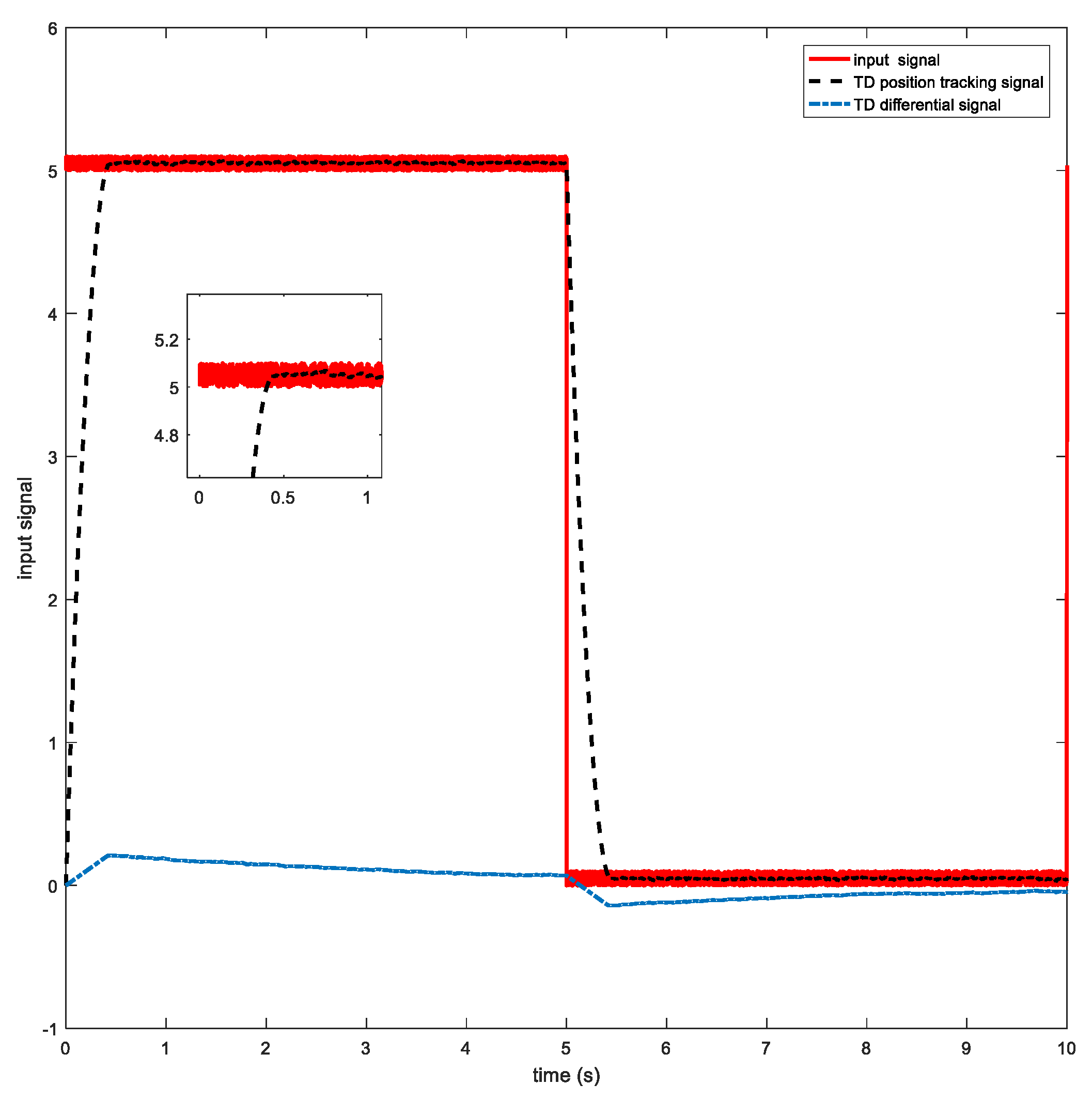
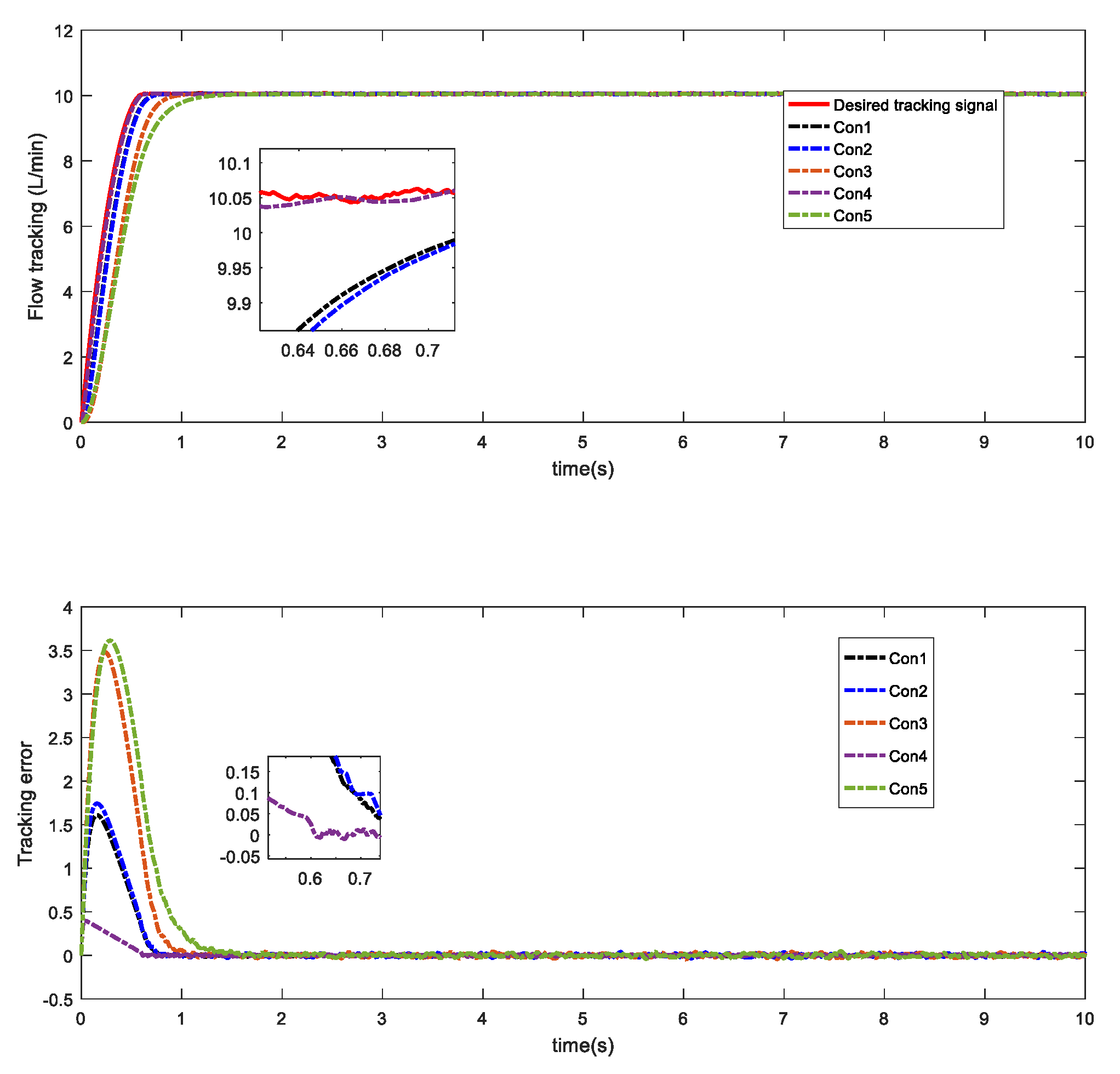
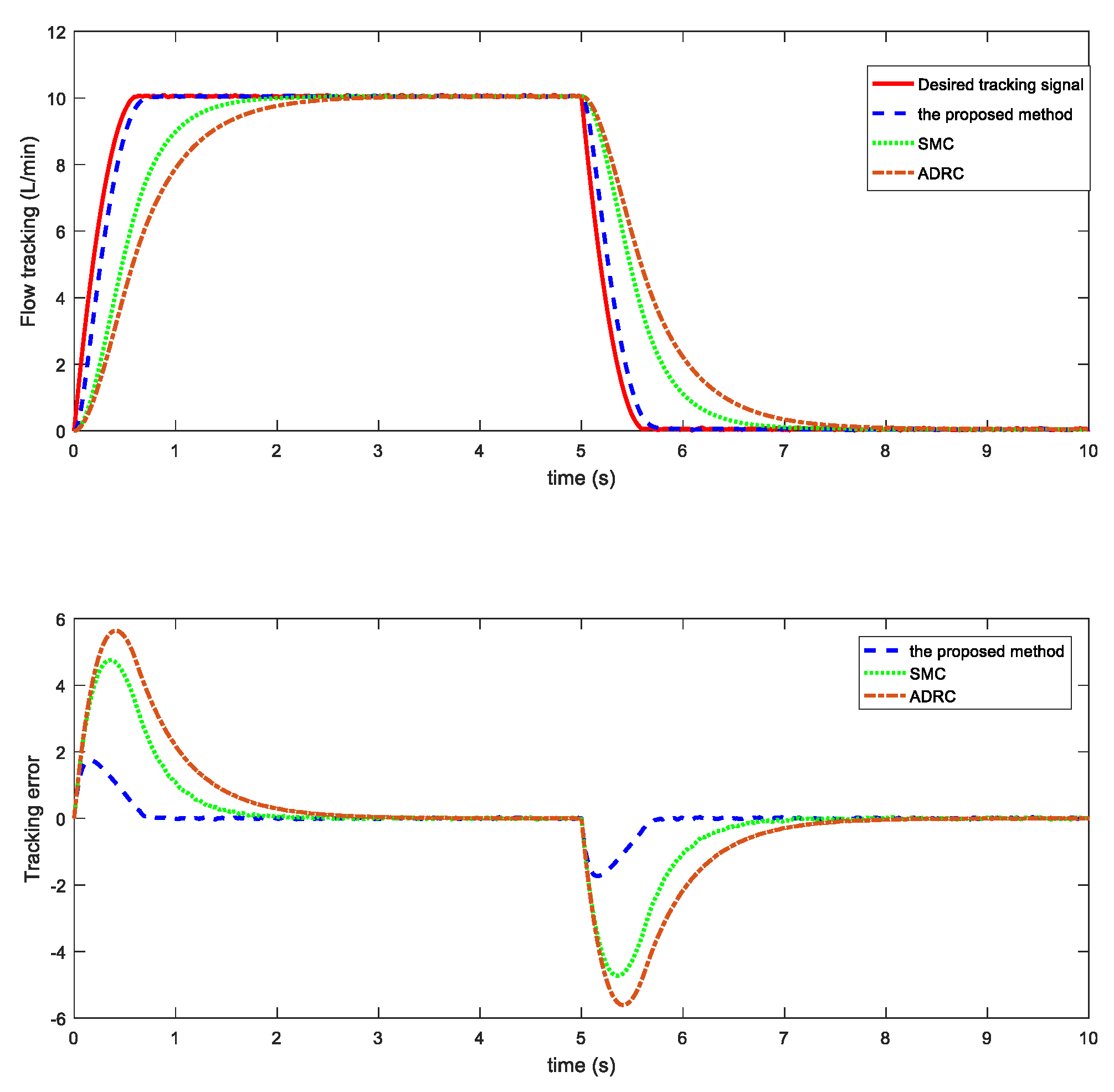
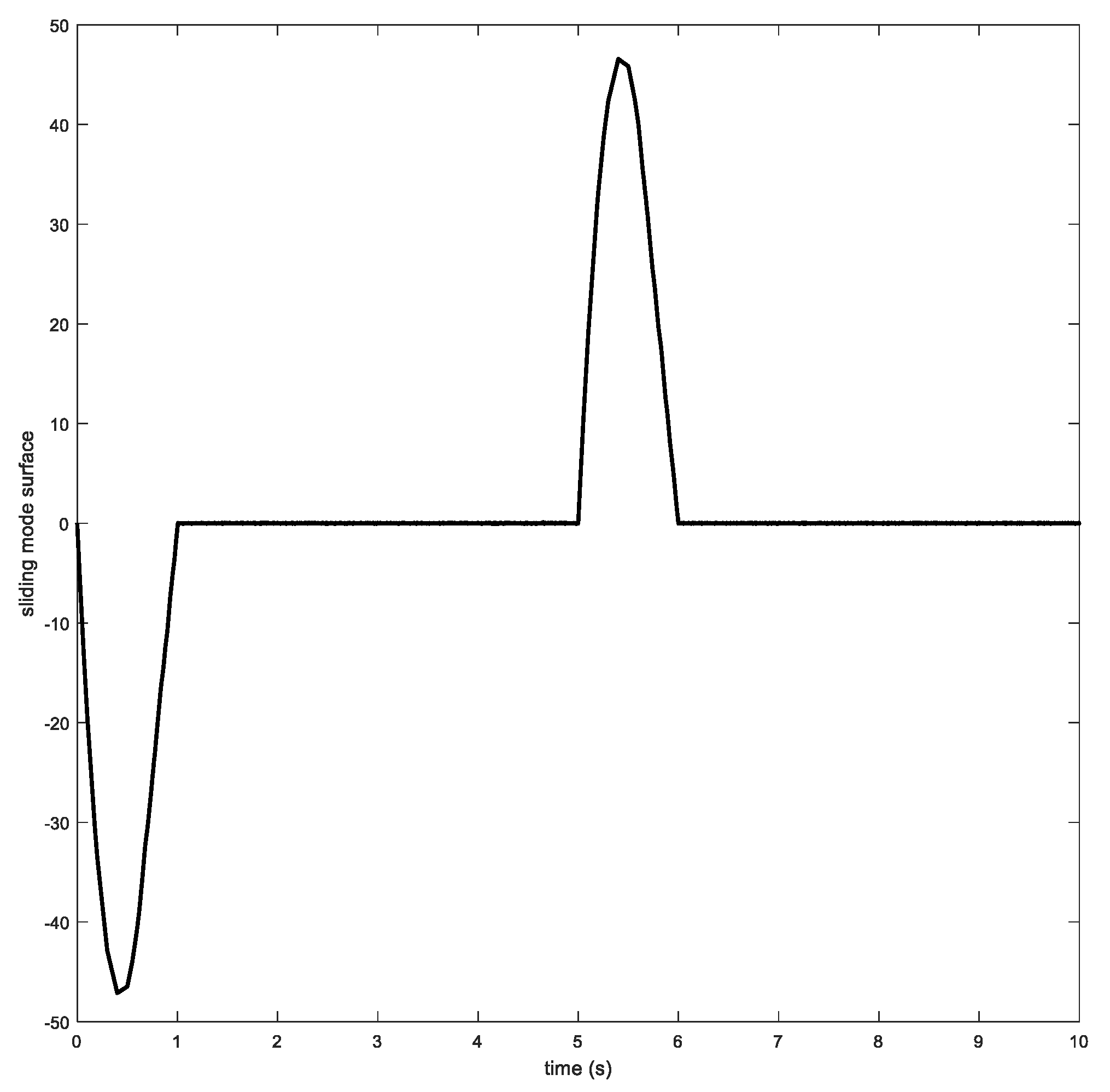
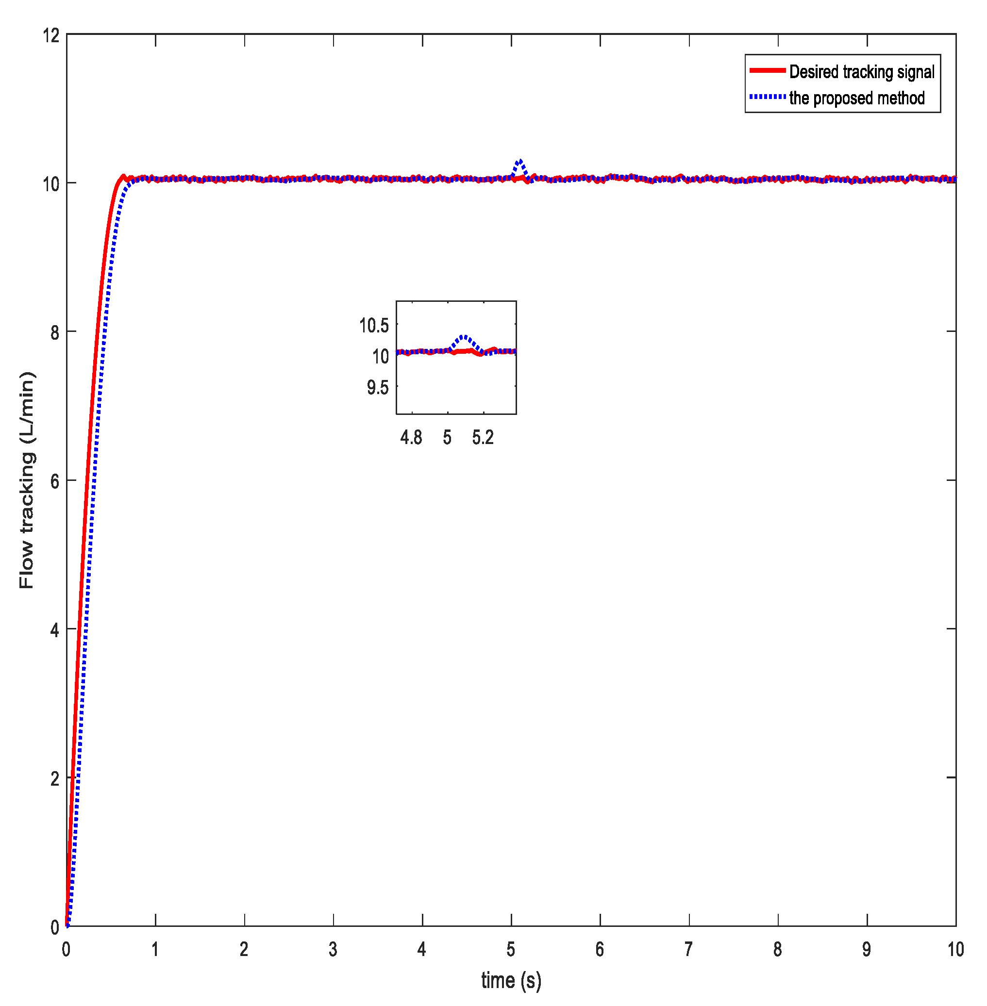
4. Simulation Analysis

For the flow dosing stage of the particleboard glue mixing and dosing system, the purpose of simulation is to verify the effectiveness of the proposed strategy and it is conducted with Matlab2016a/Simulink. Through a lot of simulation experiments, the optimal controller parameters are obtained and tested on a GM&D-A type particleboard glue mixing and dosing device as shown in Figure 6.

In this simulation experiment, we design the controller using Equation (18) and Equation (33). Taking external disturbance into account, differential forms of the disturbance are exerted on the system. In order to make the system output signal track the desired signal more quickly and stably, the sliding mode controller parameters are chosen as $c_1=50$, $c_2=15$, $k_g=150$. The selection process is shown in Figure 7.

In Figure 7, Curve Con1 represents the parameter we chosen above. It can be seen that Con1 is the closest to the desired tracking signal except for Con4, but Con4 has obvious overshoot, which needs to be avoided in the real process and so it does not meet our requirements. In this process, the curve will be smoother and more stable as $k_g$ increases, but the response time will be slower as shown in Con5. The response time of the system will increase with the increase of $c_1$ and $c_2$, but the curve will be unstable and prone to overshoot at the same time as shown in Con4. Through a number of simulation experiments, we obtained the curve parameter of Con1 and chose it as the design of controller.

The desired glue flow has an amplitude of 10 square signals with random signal interference, and the disturbance is a compound sine wave. Compared with the traditional ADRC method and sliding mode control method, the simulation results are shown in the following figures.

In order to verify the effectiveness of the proposed method, we compare the simulation results with the sliding mode control and traditional ADRC methods. By comparing with the two control methods, the significance of combining them is illustrated as shown in Figure 8. It can be seen that the position tracking curve of the proposed method can track the desired position quickly and accurately. The simulation results show that the proposed controller can complement ADRC and ensure the robustness of the controller.

The time response of NNSO is shown in Figure 9 and so is the performance of the neural network. NN1 to NN5 represent the response curves under different neural network parameters. The parameters represented as NN1 are derived by the observer design, which is as follows: $\beta ={\left[3,3,1\right]}^T$, $\epsilon =0.001$, the centers $c_j=\left[\begin{array}{ccccccccc}-6& -4& -2& -1& 0& 1& 2& 4& 6\end{array}\right]$, the widths are given as ${\rho }_j=100$, $j=1,2,3$, the adaptive gains of the ideal weight are given as $\eta =3\times {10}^2$, $\kappa =6\times {10}^2$. It is obvious that the total disturbance can be effectively observed and eliminated by the neural network.

The time response of sliding mode surface is shown in Figure 10. The sliding surface is smooth and the system is stable.

Through the above results analysis, the disturbance of the system is effectively observed by NNSO, and then equivalent compensation is introduced into the control law. It can be seen from the simulation that the observer cannot completely eliminate the disturbance of the system. In this case, the sliding mode controller is introduced to control the observed disturbance, which greatly improves the robustness of the system. In order to further prove the anti-disturbance ability of the proposed method, a strong disturbance signal with larger amplitude is added to the system when t = 5 s. The response curve is shown in Figure 11 and Figure 12. The signal tracking curve shows that even if there is strong interference, the proposed control method can ensure the system recovers quickly to a stable state. The disturbance observation curve shows that NNSO can observe the disturbance well. After the disturbance mutation, it can continue to track it quickly and accurately. However, as shown in Figure 12, the observation error can be smaller in the short time of the disturbance mutation and the performance of the observer still has some room for improvement.

Through the analysis of the simulation results, the effectiveness of the proposed method is shown, including the ability of tracking the desired signals fast and accurately and the robustness to disturbance and noise.

5. Conclusions

In this paper, the role of glue flow tracking control in the particleboard mixing and dosing system is studied under the influence of time delays and disturbances such as insertion, pump, channel, and flow sensor. In the proposed control strategy, TD is used to process the input of noisy signals, and the NNSO is used to observe the system states and the total disturbance after the first-order approximation of the time-delay link, and sliding mode is used to further enhance the robustness to disturbance. Through strict Lyapunov analysis, it is proven that all signals in the closed-loop system are finally uniformly bounded and the tracking performance is proven. Finally, the advantages of the controller are further illustrated by numerical simulation experiments.

References

1. Kusumah, S.S.; Umemura, K.; Guswenrivo, I.; Yoshimura, T.; Kanayama, K. Utilization of sweet sorghum bagasse and citric acid for manufacturing of particleboard II: Influences of pressing temperature and time on particleboard properties. J. Wood Sci. 2017, 63, 161–172. [Google Scholar] [CrossRef] [Green Version]
2. Meng, Z.; Borja, P.; Ortega, R.; Liu, Z.; Su, H. Pid passivity-based control of port-hamiltonian systems. IEEE Trans. Autom. Control 2018, 63, 1032–1044. [Google Scholar]
3. Mahto, T.; Mukherjee, V. Fractional order fuzzy pid controller for wind energy-based hybrid power system using quasi-oppositional harmony search algorithm. IET Gener. Transm. Distrib. 2017, 11, 3299–3309. [Google Scholar] [CrossRef]
4. Li, D.; Ding, P.; Gao, Z. Fractional active disturbance rejection control. ISA Trans. 2016, 62, 109–119. [Google Scholar] [CrossRef]
5. Li, M.; Li, D.; Wang, J.; Zhao, C. Active disturbance rejection control for fractional-order system. ISA Trans. 2013, 52, 365–374. [Google Scholar] [CrossRef] [PubMed]
6. Chen, Y.; Vinagre, B.M.; Podlubny, I. Fractional order disturbance observer for robust vibration suppression. Nonlinear Dyn. 2004, 38, 355–367. [Google Scholar] [CrossRef]
7. Sondhi, S.; Hote, Y.V. Fractional order PID controller for load frequency control. Energy Convers. Manag. 2014, 85, 343–353. [Google Scholar] [CrossRef]
8. Li, W.; Hori, Y. Vibration suppression using single neuron-based PI fuzzy controller and fractional-order disturbance observer. IEEE Trans. Ind. Electron. 2007, 54, 117–126. [Google Scholar] [CrossRef]
9. David, S.A.; de Sousa, R.V.; Valentim Jr, C.A.; Tabile, R.A.; Machado, J.A.T. Fractional PID controller in an active image stabilization system for mitigating vibration effects in agricultural tractors. Comput. Electron. Agric. 2016, 131, 1–9. [Google Scholar] [CrossRef]
10. Ye, Y.; Yue, Z.; Gu, B. Adrc control of a 6-dof parallel manipulator for telescope secondary mirror. J. Instrum. 2017, 12, T03006. [Google Scholar] [CrossRef]
11. Zhao, C.; Li, D.; Cui, J.; Tian, L. Decentralized low-order adrc design for mimo system with unknown order and relative degree. Pers. Ubiquitous Comput. 2018, 22, 1–18. [Google Scholar] [CrossRef]
12. Yang, J.; Cui, H.; Li, S.; Zolotas, A. Optimized active disturbance rejection control for dc-dc buck converters with uncertainties using a reduced-order gpi observer. IEEE Trans. Circ. Syst. I Regul. Pap. 2018, 65, 832–841. [Google Scholar] [CrossRef] [Green Version]
13. Zhang, D.; Duan, H.; Yang, Y. Active disturbance rejection control for small unmanned helicopters via levy flight-based pigeon-inspired optimization. Aircr. Eng. Aerosp. Technol. 2017, 89, 946–952. [Google Scholar] [CrossRef] [Green Version]
14. Han, J. From PID to Active Disturbance Rejection Control. IEEE Trans. Ind. Electron. 2009, 56, 900–906. [Google Scholar] [CrossRef]
15. Rongxin, C.; Lepeng, C.; Chenguang, Y.; Mou, C. Correction to extended state observer-based integral sliding mode control for an underwater robot with unknown disturbances and uncertain nonlinearities. IEEE Trans. Ind. Electron. 2018, 66, 8279–8280. [Google Scholar]
16. Peng, Z.; Wang, J. Output-feedback path-following control of autonomous underwater vehicles based on an extended state observer and projection neural networks. IEEE Trans. Syst. Man Cybern. Syst. 2017, 48, 535–544. [Google Scholar] [CrossRef]
17. Wang, C.; Zuo, Z.; Qi, Z.; Ding, Z. Predictor-based extended-state-observer design for consensus of mass with delays and disturbances. IEEE Trans. Cybern. 2018, 49, 1259–1269. [Google Scholar] [CrossRef]
18. Hua, C.C.; Wang, K.; Chen, J.N.; You, X. Tracking differentiator and extended state observer-based nonsingular fast terminal sliding mode attitude control for a quadrotor. Nonlinear Dyn. 2018, 94, 1–12. [Google Scholar] [CrossRef]
19. Liu, Z.; Wang, Y.; Liu, S.; Li, Z.; Zhang, H.; Zhang, Z. An approach to suppress low-frequency oscillation by combining extended state observer with model predictive control of emus rectifier. IEEE Trans. Power Electron. 2019. Available online: https://www.researchgate.net/publication/330432768 (accessed on 2 December 2019). [CrossRef]
20. Liu, Y.J.; Tong, S.; Li, D.J.; Gao, Y. Fuzzy adaptive control with state observer for a class of nonlinear discrete-time systems with input constraint. IEEE Trans. Fuzzy Syst. 2015, 24, 1147–1158. [Google Scholar] [CrossRef]
21. Sanz, R.; Garcia, P.; Fridman, E.; Albertos, P. Rejection of mismatched disturbances for systems with input delay via a predictive extended state observer. Int. J. Robust Nonlinear Control 2018, 28, 2457–2467. [Google Scholar] [CrossRef]
22. Long, L.; Si, T. Small-gain technique-based adaptive NN control for switched pure-feedback nonlinear systems. IEEE Trans. Cybern. 2018, 49, 1873–1884. [Google Scholar] [CrossRef] [PubMed]
23. Zhang, Y.; Liu, Y.; Liu, L. Adaptive Finite-Time NN Control for 3-DOF Active Suspension Systems with Displacement Constraints. IEEE Access 2019, 7, 13577–13588. [Google Scholar] [CrossRef]
24. Xing, H.L.; Jeon, J.H.; Park, K.C.; Oh, I.K. Active disturbance rejection control for precise position tracking of ionic polymer–metal composite actuators. IEEE/ASME Trans. Mechatron. 2011, 18, 86–95. [Google Scholar] [CrossRef]
25. Li, R.G.; Wu, H.N. Secure communication on fractional-order chaotic systems via adaptive sliding mode control with teaching–learning–feedback-based optimization. Nonlinear Dyn. 2019, 95, 1221–1243. [Google Scholar] [CrossRef]
26. Yang, Q.; Saeedifard, M.; Perez, M.A. Sliding mode control of the modular multilevel converter. IEEE Trans. Ind. Electron. 2018, 66, 887–897. [Google Scholar] [CrossRef]
27. Karami-Mollaee, A.; Tirandaz, H.; Barambones, O. On dynamic sliding mode control of nonlinear fractional-order systems using sliding observer. Nonlinear Dyn. 2018, 92, 1379–1393. [Google Scholar] [CrossRef]
28. Guo, B.Z.; Jin, F.F. The active disturbance rejection and sliding mode control approach to the stabilization of the Euler–Bernoulli beam equation with boundary input disturbance. Automatica 2013, 49, 2911–2918. [Google Scholar] [CrossRef]
29. Shilin, A.A.; Bukreev, V.G. Linearization of a heat-transfer system model with approximation of transport time delay. Therm. Eng. 2014, 61, 741–746. [Google Scholar] [CrossRef]
30. Ge, S.S.; Hang, C.C.; Lee, T.H.; Zhang, T. Stable Adaptive Neural Network Control; Springer Science Business Media: Berlin, Germany, 2013; Volume 13. [Google Scholar]
31. Miroslav, K.; Kanellakopoulos, I.; Petar, V. Nonlinear and Adaptive Control Design; Wiley: New York, NY, USA, 1995. [Google Scholar]
32. Dong, Q.; Yongkai, L.; Zhang, Y.; Gao, S.; Chen, T. Improved adrc with ilc control of a ccd-based tracking loop for fast steering mirror system. IEEE Photonics J. 2018, 10, 1–14. [Google Scholar] [CrossRef]
33. Ioannou, P.A.; Sun, J. Robust Adaptive Control; Prentice-Hall: Englewood Cliffs, NJ, USA, 1996. [Google Scholar]
Figure 1. Schematic diagram of glue mixing system. (1. Curing agent; 2. Waterproof agent; 3. Curing buffer agent; 4. Water; 5. Liquid level detector; 6. Quantitative barrel; 7. Electronic control throttle valve; 8. Feeding tube; 9. Cylinder; 10. Ball valve; 11. Blanking tube; 12. Agitator; 13. Glue mixing case).
Algorithms 12 00259 g001
Figure 2. Particleboard glue mixing and dosing system.
Algorithms 12 00259 g002
Figure 3. The basic structure of the flow control system.
Algorithms 12 00259 g003
Figure 4. Time response of the tracking differentiator (TD).
Algorithms 12 00259 g004
Figure 5. Configuration of the RBF neural network.
Algorithms 12 00259 g005
Figure 6. GM&D-A type particleboard glue mixing and dosing device.
Algorithms 12 00259 g006
Figure 7. Time response of glue flow tracking and tracking error.
Algorithms 12 00259 g007
Figure 8. Time response of glue flow tracking and tracking error.
Algorithms 12 00259 g008
Figure 9. Time response of the neural network state observer (NNSO) of active disturbance rejection control (ADRC).
Algorithms 12 00259 g009
Figure 10. Time response of the sliding mode surface.
Algorithms 12 00259 g010
Figure 11. Time response of the flow tracking.
Algorithms 12 00259 g011
Figure 12. Time response of disturbance observation.
Algorithms 12 00259 g012