Complexity of Hamiltonian Cycle Reconfiguration

Abstract

The Hamiltonian cycle reconfiguration problem asks, given two Hamiltonian cycles $C_0$ and $C_t$ of a graph G, whether there is a sequence of Hamiltonian cycles $C_0,C_1,\dots ,C_t$ such that $C_i$ can be obtained from $C_{i-1}$ by a switch for each i with $1\le i\le t$, where a switch is the replacement of a pair of edges $uv$ and $wz$ on a Hamiltonian cycle with the edges $uw$ and $vz$ of G, given that $uw$ and $vz$ did not appear on the cycle. We show that the Hamiltonian cycle reconfiguration problem is PSPACE-complete, settling an open question posed by Ito et al. (2011) and van den Heuvel (2013). More precisely, we show that the Hamiltonian cycle reconfiguration problem is PSPACE-complete for chordal bipartite graphs, strongly chordal split graphs, and bipartite graphs with maximum degree 6. Bipartite permutation graphs form a proper subclass of chordal bipartite graphs, and unit interval graphs form a proper subclass of strongly chordal graphs. On the positive side, we show that, for any two Hamiltonian cycles of a bipartite permutation graph and a unit interval graph, there is a sequence of switches transforming one cycle to the other, and such a sequence can be obtained in linear time.

1. Introduction

A reconfiguration problem asks, given two feasible solutions of a combinatorial problem together with some transformation rules between the solutions, whether there is a step-by-step transformation from one solution to the other such that all intermediate states are also feasible. The reconfiguration problems have attracted much attention recently because of their applications as well as theoretical interest. See, for example, a survey [1] and references of [2,3].

In this paper, we study a reconfiguration problem for Hamiltonian cycles. A Hamiltonian cycle of a graph is a cycle that contains all the vertices of the graph. Given two Hamiltonian cycles $C_0$ and $C_t$ of a graph G, the Hamiltonian cycle reconfiguration problem asks whether there is a sequence of Hamiltonian cycles $C_0,C_1,\dots ,C_t$ such that $C_i$ and $C_{i+1}$ differ in two edges for each i with $0\le i<t$. Such a sequence of Hamiltonian cycles is called a reconfiguration sequence. The Hamiltonian cycle reconfiguration problem also can be defined in terms of the transformation rule, which is called switch (Switches are also used for sampling and counting perfect matchings [4,5] and transforming graphs with the same degree sequence ([6,7], p.46)). Let C be a Hamiltonian cycle of a graph G. A switch is the replacement of a pair of edges $uv$ and $wz$ on C with the edges $uw$ and $vz$ of G, given that $uw$ and $vz$ did not appear on C. The Hamiltonian cycle reconfiguration problem asks whether there is a sequence of switches transforming one cycle to the other such that all intermediate cycles are also Hamiltonian.

The complexity of the reconfiguration problem for Hamiltonian cycles has been implicitly posed as an open question by Ito et al. [8] (Precisely, they asked the complexity of the reconfiguration of the travelling salesman problem, which is a generalization of the Hamiltonian cycle problem) and revisited by van den Heuvel [1]. The Hamiltonian cycle problem, which asks whether a given graph has a Hamiltonian cycle, is one of the well-known NP-complete problems [9], but the complexity of its reconfiguration version still seems to be open.

1.1. Our Contribution

In this paper, we show that the Hamiltonian cycle reconfiguration problem is PSPACE-complete, even for chordal bipartite graphs, strongly chordal split graphs, and bipartite graphs with maximum degree 6. Our reduction for PSPACE-hardness follows from the reduction by Müller [10] for proving the NP-hardness of the Hamiltonian cycle problem for chordal bipartite graphs. However, while Müller shows a polynomial-time reduction from the satisfiability problem, we show a reduction from the nondeterministic constraint logic problem [11], which is used to show the PSPACE-hardness of some reconfiguration problems [11,12].

Unit interval graphs form a proper subclass of strongly chordal graphs, and bipartite permutation graphs form a proper subclass of chordal bipartite graphs (See [13] for example). A Hamiltonian cycle of a unit interval graph and a bipartite permutation graph can be obtained in linear time [14,15,16,17]. On the positive side, we show that, for any two Hamiltonian cycles of a unit interval graph and a bipartite permutation graph, there is a sequence of switches transforming one cycle to the other. Moreover, we show that such a sequence can be obtained in linear time. In order to show these results, we introduce the canonical Hamiltonian cycle (canonical cycle for short) of a unit interval graph and a bipartite permutation graph, using vertex ordering characterizations of these graphs [14,17]. We then show that each Hamiltonian cycle of a unit interval graph (resp. a bipartite permutation graph) can be transformed into the canonical cycle with at most $n-2$ switches (resp. at most $n-3$ switches), where n is the number of vertices of the graph. It follows that, for any two Hamiltonian cycles of a unit interval graph (resp. a bipartite permutation graph), there is a sequence of at most $2n-4$ switches (resp. at most $2n-6$ switches) from one cycle to the other.

1.2. Notation

In this paper, we will deal only with finite graphs having no loops and multiple edges. Unless stated otherwise, graphs are assumed to be undirected, but we also deal with directed graphs. We write $uv$ for the undirected edge joining a vertex u and a vertex v, and we write $(u,v)$ for the directed edge from u to v. For a graph $G=(V,E)$, we sometimes write $V\left(G\right)$ for the vertex set V of G and write $E\left(G\right)$ for the edge set E of G.

An independent set of a graph $G=(V,E)$ is a subset $S\subseteq V$ such that $uv\notin E$ for any two vertices $u,v\in S$. A graph G is a bipartite graph if its vertex set V can be partitioned into two independent set U and W. The independent sets U and W are called color classes of G, and the pair $(U,W)$ is called bipartition of G. We sometimes use the notation $G=(U,W,E)$ for the bipartite graph with bipartition $(U,W)$.

An orientation of an undirected graph $G=(V,E)$ is a graph obtained from G by orienting each edge in E, that is, replacing each edge $uv\in E$ with either $(u,v)$ or $(v,u)$. An oriented graph is an orientation of some graph. Notice that an oriented graph contains no pair of edges $(u,v)$ and $(v,u)$ for some vertices $u,v$. We will denote an orientation of a graph only by its edge set, since the vertex set is clear from the context.

2. PSPACE-Completeness

We can observe that the Hamiltonian cycle reconfiguration problem is in PSPACE ([8], Theorem 1). In this section, we show the reduction from the nondeterministic constraint logic problem, which is known to be PSPACE-complete [11], to the Hamiltonian cycle reconfiguration problem.

2.1. Nondeterministic Constraint Logic

Let G be a 3-regular graph with edge weights among $\{1,2\}$. A vertex of G is an AND vertex if exactly one incident edge has weight 2, and a vertex of G is an OR vertex if all the incident edges have weight 2. A graph G is a constraint graph if it consists of only AND vertices and OR vertices. An orientation F of G is legal if for every vertex v of G, the sum of weights of in-coming edges of v is at least 2. A legal move from a legal orientation is the reversal of a single edge that results in another legal orientation. 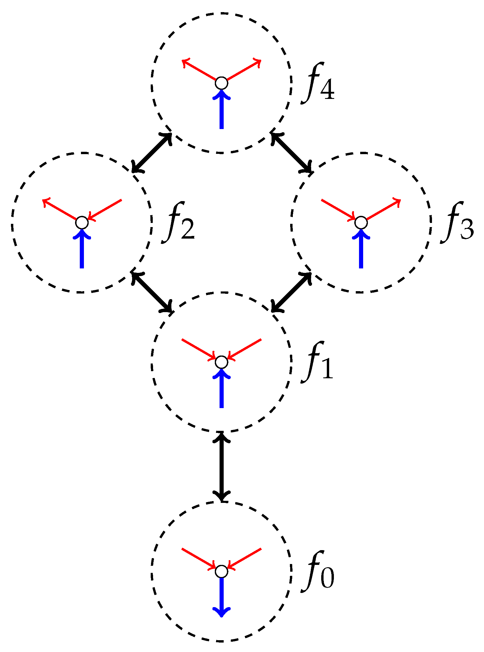Figure 1 illustrates all the possible orientations of edges incident to an AND vertex. We can also verify that all the possible legal move of an incident edge of the AND vertex are those depicted by the arrows in Figure 1. Given a constraint graph G and two legal orientation $F_0$ and $F_t$ of G, the nondeterministic constraint logic problem asks whether there is a sequence of legal orientations $F_0,F_1,\dots ,F_t$ such that $F_i$ is obtained from $F_{i-1}$ by a legal move for each i with $1\le i\le t$. Such a sequence of legal orientations is called a reconfiguration sequence. The nondeterministic constraint logic problem is known to be PSPACE-complete even if the constraint graph is planar [11]. See [18] for more information on constraint logic.

Figure 1. All the possible orientations of edges incident to an AND vertex, where (blue) thick arrows denote the edges with weight 2, and (red) thin arrows denote the edges with weight 1. Each dotted circle represents a possible orientation of the edges, and two circles are joined by an arrow if one is obtained from the other by reversing the direction of a single edge.

For convenience of the reduction, we define a problem slightly different from the nondeterministic constraint logic problem. Let G be a bipartite graph with bipartition $(A,B)$ such that every vertex of A has degree 3 and every vertex of B has degree 2 or 3. The graph G has edge weights among $\{1,2\}$ such that for every vertex of A, exactly one incident edge has weight 2. An orientation F of G is legal if

• for every vertex $v\in A$, the sum of weights of in-coming edges of v is at least 2, and
• every vertex of B has one or two in-coming edges, but at most one vertex of B has two in-coming edges.

A legal move from a legal orientation is the reversal of a single edge that results in another legal orientation. Notice that, in the legal moves, the vertices of A behave in the same way as the AND vertices of the nondeterministic constraint logic problem, that is, as shown in Figure 1. Given such a bipartite graph G and two legal orientation $F_0$ and $F_t$ of G, the problem $\Pi$ asks whether there is a sequence of legal orientations $F_0,F_1,\dots ,F_t$ such that $F_i$ is obtained from $F_{i-1}$ by a legal move for each i with $1\le i\le t$. We further add a constraint to the instance of the problem $\Pi$ so that every vertex of B has exactly one in-coming edge in $F_0$ and $F_t$.

Lemma 1.

The problem Π is PSPACE-complete.

Proof. 

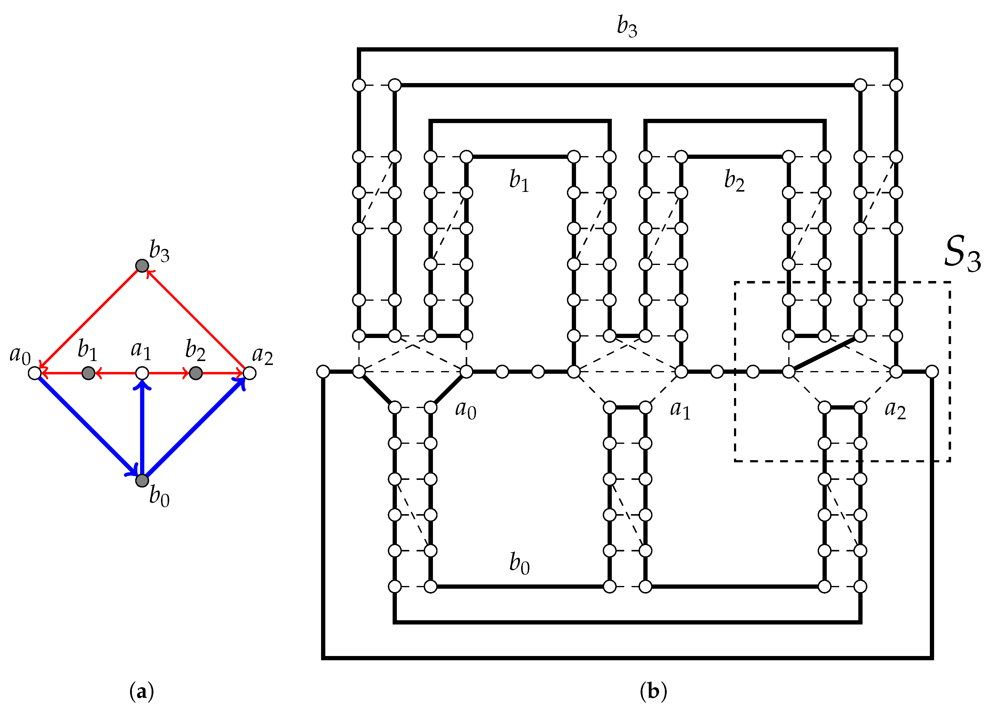
We can observe that the problem $\Pi$ is in PSPACE ([8], Theorem 1). We thus show a polynomial-time reduction from the nondeterministic constraint logic problem. Let $(G,F_0,F_t)$ be an instance of the problem, that is, G is a constraint graph, consisting of AND vertices and OR vertices, and $F_0$ and $F_t$ are two legal orientations of G. We construct an instance $(G^{\prime },F_0^{\prime },F_t^{\prime })$ of the problem $\Pi$ such that $(G,F_0,F_t)$ is a yes-instance if and only if $(G^{\prime },F_0^{\prime },F_t^{\prime })$ is a yes-instance.

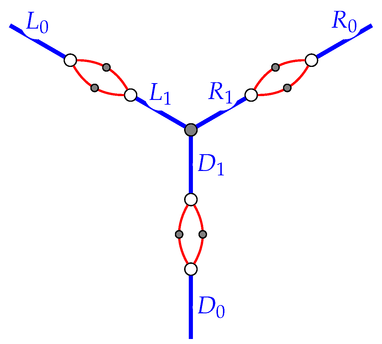
Let $G^{″}$ be the bipartite graph obtained from G by replacing each edge $uv$ with two edges $uw$ and $wv$ so that $uw$ and $wv$ have the same weight as $uv$, where w is a newly added vertex. The bipartite graph $G^{\prime }$ with bipartition $(A,B)$ is obtained from $G^{″}$ by replacing each OR vertex with a subgraph shown in Figure 2, where A consists of the AND vertices of G and the white points in the subgraphs (see Figure 2) while B consists of the newly added vertices of $G^{″}$ and the gray points in the subgraphs. We can check that all the vertices of A are incident to one weight-2 edge and two weight-1 edges.

Figure 2. The reduction from the nondeterministic constraint logic problem to the problem $\Pi$. White points denote the vertices of A, and gray points denote the vertices of B. Thick (blue) lines denote the edges with weight 2, and thin (red) lines denote the edges with weight 1.

Let F be a legal orientation of G. We define a legal orientation $F^{\prime }$ of $G^{\prime }$associated withF. Let $F^{″}$ be the orientation of $G^{″}$ obtained from F by replacing each edge $(u,v)\in F$ with two edges $(u,w)$ and $(w,v)$, where w is the newly added vertex. Let $F^{″\prime }$ be an orientation of $G^{\prime }$ obtained from $F^{″}$ by replacing each OR vertex with the subgraph in Figure 2 such that if L is directed inward (resp. outward) in $F^{″}$ then the edges $L_0$ and $L_1$ and the weight-1 edges between them are directed inward (resp. outward) in $F^{″\prime }$ (and similarly for the edges R and D). The legal orientation $F^{\prime }$ is obtained from $F^{″\prime }$ by reversing the direction of the edges incident to the OR vertices so that exactly one edge of $\{L_1,R_1,D_1\}$ is directed inward for each OR vertex. Notice that at least one edge of $\{L_1,R_1,D_1\}$ can be directed inward, since at least one edge of $\{L,R,D\}$ is directed inward in F. We can see that $F^{\prime }$ has no vertex of B having two in-coming edges. The legal orientations $F_0^{\prime }$ and $F_t^{\prime }$ are the orientations associated with $F_0$ and $F_t$, respectively. This completes the construction of the instance $(G^{\prime },F_0^{\prime },F_t^{\prime })$ of the problem $\Pi$.

Assume that there is a reconfiguration sequence $F_0,F_1,\dots ,F_t$ from $F_0$ to $F_t$. Let $F_i^{\prime }$ be a legal orientation of $G^{\prime }$ associated with $F_i$. If $F_{i+1}$ is obtained from $F_i$ by a legal move of an edge joining two AND vertices, we have a reconfiguration sequence from $F_i^{\prime }$ to $F_{i+1}^{\prime }$. Suppose that $F_{i+1}$ is obtained by a legal move of an edge incident to an OR vertex. Let L, R, and D be the edges incident to the OR vertex. We assume without loss of generality that $F_{i+1}$ is obtained by a legal move of the edge L. When L is directed inward in $F_i$, the edge L is directed outward in $F_{i+1}$, and thus the edges R or D are directed inward in $F_i$. Hence, in $F_i^{\prime }$ the edge $R_1$ or $D_1$ can be directed inward (see Figure 2). Therefore, the edges $L_0$ and $L_1$ together with the weight-1 edges between them can be directed outward to obtain $F_{i+1}^{\prime }$. When L is directed outward in $F_i$ and inward in $F_{i+1}$, in $F_i^{\prime }$ the edges $L_0$ and $L_1$ together with the weight-1 edges between them can be directed inward to obtain $F_{i+1}^{\prime }$. Since there is a reconfiguration sequence from $F_i^{\prime }$ to $F_{i+1}^{\prime }$ for any i with $0\le i<t$, the instance $(G^{\prime },F_0^{\prime },F_t^{\prime })$ is a yes-instance if $(G,F_0,F_t)$ is a yes-instance. Notice that, in the subgraph shown in Figure 2, if two edges of $\{L_0,R_0,D_0\}$ are directed outward, then the remaining edge must be directed inward. Thus, a reconfiguration sequence from $F_0$ to $F_t$ can be obtained from a reconfiguration sequence from $F_0^{\prime }$ to $F_t^{\prime }$. It follows that the instance $(G,F_0,F_t)$ is a yes-instance if $(G^{\prime },F_0^{\prime },F_t^{\prime })$ is a yes-instance.

Since the graph $G^{\prime }$ and the legal orientations $F_0^{\prime }$ and $F_t^{\prime }$ can be obtained in polynomial time, we have the claim. □

We can further see from the proof of Lemma 1 that the problem $\Pi$ is PSPACE-complete for planar graphs, since the nondeterministic constraint logic problem is PSPACE-complete even if the constraint graph is planar [11]. We can also see the following observation, which we will use in the proof of Lemma 2.

Proposition 1.

Let $(G,F_0,F_t)$ be an instance of the problem Π with a reconfiguration sequence $F_0,F_1,\dots ,F_t$ from $F_0$ to $F_t$. If i is even, then $F_i$ has no vertex of B having two in-coming edges, while $F_i$ has one vertex of B having two in-coming edges if otherwise. If a vertex $b_i\in B$ has two in-coming edges $(a_i,b_i)$ and $(a_i^{\prime },b_i)$ in $F_i$, then we can assume without loss of generality that $F_i$ is obtained from $F_{i-1}$ by reversing the direction of the edge $a_i{b}_i$, while $F_{i+1}$ is obtained from $F_i$ by reversing the direction of the edge $a_i^{\prime }{b}_i$.

Proof. 

Let $F_i$ be a legal orientation such that every vertex of B has exactly one in-coming edge. Suppose that $F_{i+1}$ is obtained from $F_i$ by reversing the direction of an edge $a_i{b}_i$, where $a_i$ and $b_i$ are the vertices of A and B, respectively. Since all the vertices of B has one in-coming edge in $F_i$, we have $(b_i,a_i)\in F_i$ and $(a_i,b_i)\in F_{i+1}$. Now, $b_i$ has two in-coming edges in $F_{i+1}$. Let $(a_i^{\prime },b_i)\in F_i$ be the in-coming edge of $b_i$ in $F_i$. If we reverse the direction of an edge other than $a_i{b}_i$ or $a_i^{\prime }{b}_i$, then the orientation is no longer legal. Thus, we can reverse the direction of either $a_i{b}_i$ or $a_i^{\prime }{b}_i$ to obtain $F_{i+2}$, in which every vertex of B has exactly one in-coming edge. However, if we reverse the direction of $a_i{b}_i$, then we have the same orientation as $F_i$. Thus, we can assume without loss of generality that $(a_i^{\prime },b_i)\in F_{i+1}$ and $(b_i,a_i^{\prime })\in F_{i+2}$. Now, we have the claim. □

2.2. Reduction

Let $(G,F_0,F_t)$ be an instance of the problem $\Pi$. In this section, we construct a reduction graph H together with two Hamiltonian cycles $C_0$ and $C_t$ such that there is a reconfiguration sequence from $F_0$ to $F_t$ if and only if there is a reconfiguration sequence from $C_0$ to $C_t$. That is, $(G,F_0,F_t)$ is a yes-instance if and only if $(H,C_0,C_t)$ is a yes-instance of the Hamiltonian cycle reconfiguration problem.

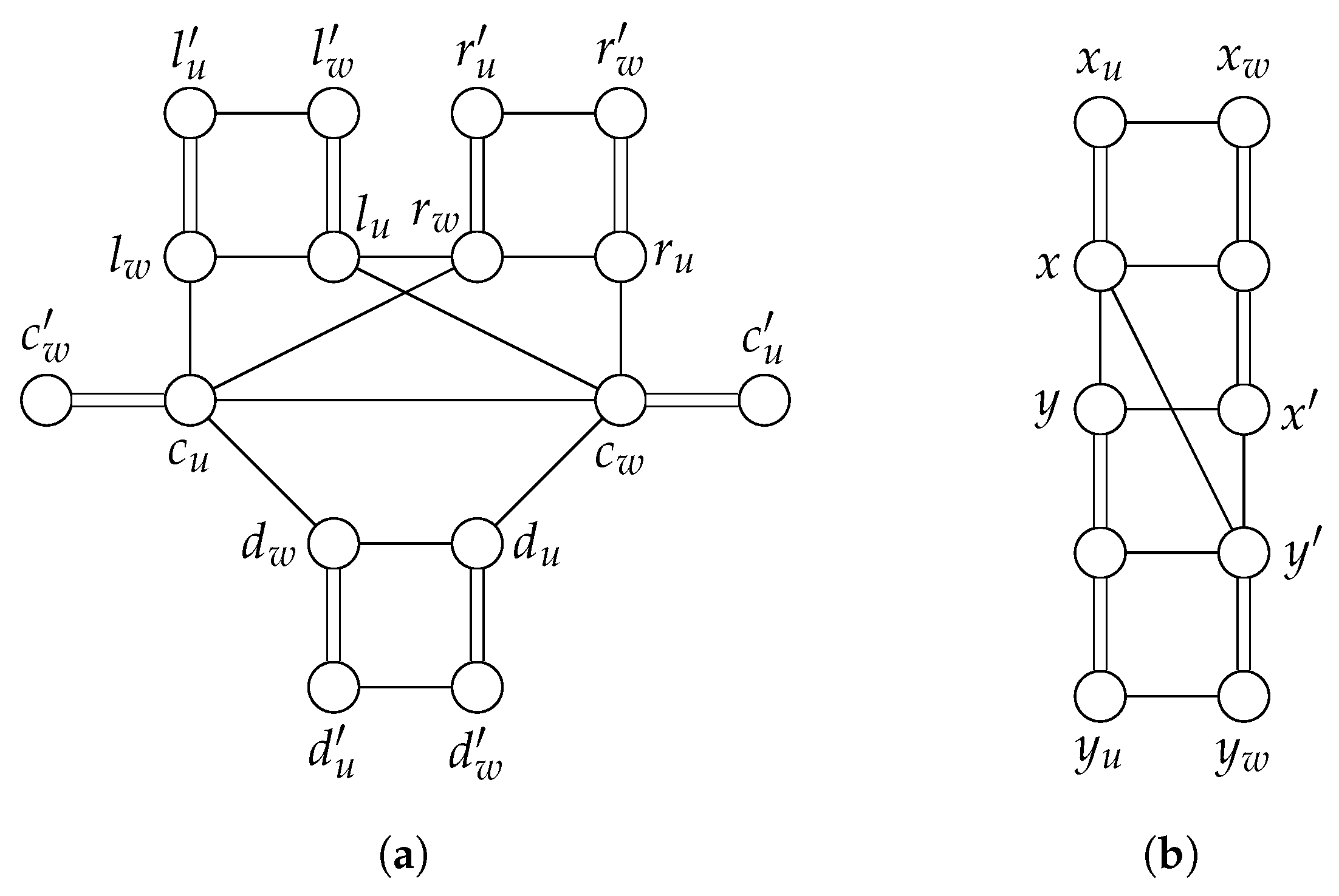
We use three types of gadgets corresponding to the vertices in A, the vertices in B, and the edges of G. A gadget for a vertex in A and a gadget for an edge of G is shown in Figure 3a,b respectively. Double lines in the figures denote edges with ears, where an ear of an edge $uw$ is a path of length 3 joining u and w. Recall that, in the legal moves, the vertices in A behave in the same way as the AND vertices. We thus refer to the gadgets for the vertices in A as AND gadgets. Let b be a vertex in B of degree k, and recall that k is 2 or 3. A gadget for b is a cycle $(u_0,w_0,u_1,w_1,\dots ,u_{k-1},w_{k-1})$ of length $2k$ such that the edge $w_i{u}_{i+1}$ has a ear for each i with $0\le i<k$ (indices are modulo k).

Figure 3. Gadgets. Double lines denote edges with ears. (a) an AND gadget; (b) an edge gadget.

We construct the reduction graph H from G as follows: (1) Let a be a vertex in A, and let $e_l,e_r,e_d$ be the edges of G incident to a such that $e_l$ and $e_r$ have weight 1 and $e_d$ has weight 2. We identify the vertices $l_u^{\prime }$ and $l_w^{\prime }$ of the gadget for a with the vertices $x_u$ and $x_w$ of the gadget for $e_l$, respectively. Similarly, we identify the vertices $r_u^{\prime }$ and $r_w^{\prime }$ of the gadget for a with the vertices $x_u$ and $x_w$ of the gadget for $e_r$, respectively. Moreover, we identify the vertices $d_u^{\prime }$ and $d_w^{\prime }$ of the gadget for a with the vertices $x_u$ and $x_w$ of the gadget for $e_d$, respectively. (2) Let b be a vertex in B of degree k, and let $e_0,e_1,\dots ,e_{k-1}$ be the edges of G incident to b. We identify, for each i with $0\le i<k$, the vertices $u_i$ and $w_i$ of the gadget for b with the vertices $y_u$ and $y_w$ of the gadget for $e_i$, respectively. (3) We finally concatenate the gadgets for the vertices in A cyclically using edges with ears joining the vertices $c_u^{\prime }$ and $c_w^{\prime }$ of the gadgets.

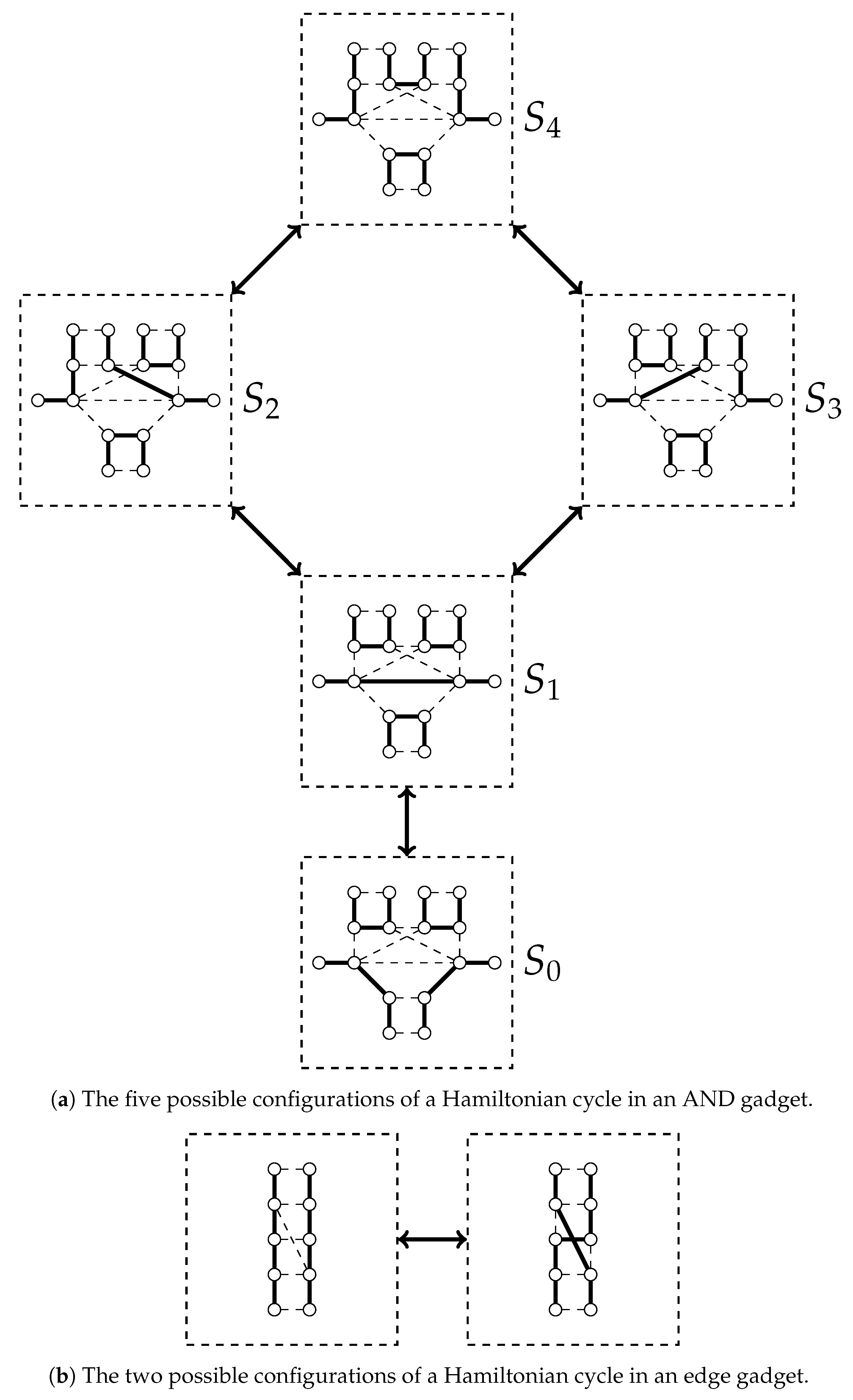
Before describing the construction of the Hamiltonian cycles $C_0$ and $C_t$, we consider the possible configurations of a Hamiltonian cycle of the reduction graph H passing through the gadgets. We will show that all the possible configurations in an AND gadget and an edge gadget are shown in Figure 4a,b, respectively. We can also verify that all the possible transformations of Hamiltonian cycles by a single switch occurred in a gadget are those depicted by the arrows in the figures. Let C be a Hamiltonian cycle. We first consider the configurations of C in an AND gadget. The Hamiltonian cycle C passes through all the edges on the ears, since interior vertices of an ear has degree 2. Thus, C passes through any of the edges $c_u{d}_w$, $c_u{c}_w$, $c_u{r}_w$, or $c_u{l}_w$. We also have that C does not pass through the edges $l_u^{\prime }{l}_w^{\prime }$, $r_u^{\prime }{r}_w^{\prime }$, or $d_u^{\prime }{d}_w^{\prime }$, since when we construct the reduction graph H the vertices $l_u^{\prime }$, $l_w^{\prime }$, $r_u^{\prime }$, $r_w^{\prime }$, $d_u^{\prime }$ and $d_w^{\prime }$ are identified with the vertices of the edge gadgets incident to the edges with ears. Suppose that C passes through $c_u{d}_w$. Since C cannot pass through $d_u{d}_w$, it passes through $d_u{c}_w$. Since C cannot pass through $c_u{l}_w$, it passes through $l_u{l}_w$. Since C cannot pass through $l_u{r}_w$, it passes through $r_u{r}_w$, and we have the configuration $S_0$ in Figure 4a. Suppose that C passes through $c_u{c}_w$. Since C cannot pass through $c_u{d}_w$, it passes through $d_u{d}_w$. Since C cannot pass through $c_u{l}_w$, it passes through $l_u{l}_w$. Since C cannot pass through $l_u{r}_w$, it passes through $r_u{r}_w$, and we have the configuration $S_1$ in Figure 4a. Suppose that C passes through $c_u{r}_w$. Since C cannot pass through $c_u{d}_w$, it passes through $d_u{d}_w$. Since C cannot pass through $c_u{l}_w$, it passes through $l_u{l}_w$. Since C cannot pass through $r_u{r}_w$, it passes through $r_u{c}_w$, and we have the configuration $S_3$ in Figure 4a. Suppose that C passes through $c_u{l}_w$. Since C cannot pass through $c_u{d}_w$, it passes through $d_u{d}_w$. Since C cannot pass through $l_u{l}_w$, it passes through either $l_u{r}_w$ or $l_u{c}_w$. If C passes through $l_u{r}_w$, then it passes through $r_u{c}_w$ since it cannot pass through $r_u{r}_w$, and we have the configuration $S_4$ in Figure 4a. If C passes through $l_u{c}_w$, then it passes through $r_u{r}_w$ since it cannot pass through $l_u{r}_w$, and we have the configuration $S_2$ in Figure 4a. Therefore, all the possible configurations in an AND gadget are shown in Figure 4a. We next consider the configurations of the Hamiltonian cycle C in an edge gadget. Since C passes through all the edges on the ears, it passes through either $xy$ or $x{y}^{\prime }$. If C passes through $xy$ then it passes through $x^{\prime }{y}^{\prime }$, while if C passes through $x{y}^{\prime }$, then it passes through $x^{\prime }y$. We also have that C does not pass through the edges $x_u{x}_w$ or $y_u{y}_w$, since when we construct the reduction graph H the vertices $x_u$, $x_w$, $y_u$, and $y_w$ are identified with the vertices of the AND gadgets incident to the edges with ears. Therefore, all the possible configurations in an edge gadget are shown in Figure 4b.

Figure 4. All the possible configurations of a Hamiltonian cycle passing through gadgets. The edges on the cycle are indicated by thick lines, but the ears are omitted; the edges out of the cycle are indicated by dotted lines. Each dotted square represents a possible configuration, and two squares are joined by an arrow if one is obtained from the other by a single switch.

Let v be a vertex of A. We next make a correspondence between the possible configurations of a Hamiltonian cycle in the gadget for v and the possible orientations of the edges incident to v such that the configuration $S_i$ in Figure 4a corresponds to the orientation $f_i$ in Figure 1 for each $i\in \{0,1,\dots ,4\}$. We also make a correspondence between switches occurred in the gadget for v and legal moves of the edges incident to v such that switching the configuration from $S_i$ to $S_j$ in the gadget for v corresponds to the legal move from $f_i$ to $f_j$ of the edges of v, where $i,j\in \{0,1,\dots ,4\}$.

We define a legal orientation F of G associated with a Hamiltonian cycle C of H so that for each vertex $v\in A$, the edges incident to v are oriented according to the configuration of C in the gadget for v. That is, the edges of v are oriented as $f_i$ in F if the configuration of C in the gadget for v looks like $S_i$ (see Figure 1 and Figure 4a). Notice that a Hamiltonian cycle C of H has exactly one legal orientation of G associated with C, but a legal orientation F may have some Hamiltonian cycles that are associated with F, due to the two possible configurations in an edge gadget shown in Figure 4b.

Now, we construct the Hamiltonian cycle $C_0$ from $F_0$ as follows, and $C_t$ is constructed similarly from $F_t$. (1) For each vertex $v\in A$, we take the configuration in the gadget for v according to the orientations of the edges incident to v. That is, we take the configuration $S_i$ in Figure 4a for the gadget for v if the edges of v are oriented as $f_i$ in Figure 1. (2) We choose the configuration in each edge gadget arbitrarily among those in Figure 4b. (3) The remaining parts are uniquely determined, since any Hamiltonian cycle pass through all the edges on the ears. Figure 5b illustrates the Hamiltonian cycle constructed in this way from the legal orientation in Figure 5a. Recall that every vertex of B has exactly one in-coming edge in $F_0$ and $F_t$. This guarantees that $C_0$ and $C_t$ are Hamiltonian. This completes the construction of the instance $(H,C_0,C_t)$ of the Hamiltonian cycle reconfiguration problem. We remark two facts, which we use in the proof of the following lemma. First, we can see that $C_0$ and $C_t$ are associated with $F_0$ and $F_t$, respectively. Second, if every vertex of B has exactly one in-coming edge in a legal orientation F, then for any two Hamiltonian cycles that are associated with $F_t$, there is a reconfiguration sequence from one to the other, in which the switches occur only in edge gadgets.

Figure 5. (a) a legal orientation of the problem $\Pi$. White points denote the vertices of A, and gray points denote the vertices of B. Thick (blue) lines denote the edges with weight 2, and thin (red) lines denote the edges with weight 1; (b) the Hamiltonian cycle obtained from the legal orientation in Figure 5a. We take the configuration $S_3$ for the gadget for $a_2$, since the edges of $a_2$ are oriented as $f_3$ in Figure 5a. Notice that, when we replace the configuration from $S_3$ to $S_4$, we have two cycles.

Lemma 2.

The instance $(G,F_0,F_t)$ of the problem Π is a yes-instance if and only if $(H,C_0,C_t)$ of the Hamiltonian cycle reconfiguration problem is a yes-instance.

Proof. 

We first prove the if direction. Assume that there is a reconfiguration sequence $C_0,C_1,\dots ,C_t$ from $C_0$ to $C_t$. Let $F_i$ be the legal orientation of G associated with $C_i$ (Recall that a Hamiltonian cycle C of H has exactly one legal orientation associated with C). Notice that $F_i=F_{i+1}$ if and only if $C_{i+1}$ is obtained from $C_i$ by a switch occurred in an edge gadget. When $F_i=F_{i+1}$ for some i with $0\le i<t$, we remove $F_{i+1}$ from the sequence $F_0,F_1,\dots ,F_t$ to obtain the reconfiguration sequence from $F_0$ to $F_t$.

We next prove the only-if direction. Assume that there is a reconfiguration sequence $F_0,F_1,\dots ,F_t$ from $F_0$ to $F_t$. Recall that, for any two Hamiltonian cycles that are associated with $F_t$, there is a reconfiguration sequence from one to the other, since every vertex of B has exactly one in-coming edge in $F_t$. Thus, it suffices to show that for each Hamiltonian cycle $C_i$ with $0\le i<t$, there is a Hamiltonian cycle $C_{i+1}$ together with a reconfiguration sequence from $C_i$ to $C_{i+1}$, where $C_i$ and $C_{i+1}$ are Hamiltonian cycles associated with $F_i$ and $F_{i+1}$, respectively. Suppose that $F_{i+1}$ is obtained from $F_i$ by reversing the direction of an edge $a_i{b}_i$, where $a_i$ and $b_i$ are the vertices of A and B, respectively.

We first consider the case when $(b_i,a_i)\in F_i$ and $(a_i,b_i)\in F_{i+1}$. We have from Proposition 1 that $F_i$ has no vertex of B having two in-coming edges. Let C be a graph obtained from $C_i$ by switching the configuration in the gadget for $a_i$ according to the legal move. If C is a Hamiltonian cycle, the claim holds. However, there is some possibility that C is disconnected. (In Figure 5b, for example, when we replace the configuration in the gadget for $a_2$ from $S_3$ to $S_4$, we have two cycles, while, in Figure 5a, this replacement corresponds to the reversal of the edge $(b_2,a_2)$ that results in another legal orientation). In this case, we use two steps as follows: Let $C^{\prime }$ be a graph obtained from $C_i$ by switching the configuration in the edge gadget for $a_i{b}_i$ as shown in Figure 4b. Let $C^{″}$ be a graph obtained from $C^{\prime }$ by switching the configuration in the gadget for $a_i$ according to the legal move. We show that $C^{\prime }$ and $C^{″}$ are Hamiltonian cycles. Suppose that C is obtained from $C_i$ by switching edges $v_1{v}_2$ and $v_3{v}_4$ with edges $v_1{v}_3$ and $v_2{v}_4$. Suppose also that $C^{\prime }$ is obtained from C by switching edges $v_5{v}_6$ and $v_7{v}_8$ with edges $v_5{v}_7$ and $v_6{v}_8$. Since C is disconnected while $C_i$ is Hamiltonian, the vertices $v_1$, $v_2$, $v_3$, and $v_4$ appear on $C_i$ as $C_i=(v_1,v_2,\dots ,v_4,v_3,\dots )$. Since $(b_i,a_i)\in F_i$ and the switch occurs in the edge gadget, we can assume without loss of generality that the vertices $v_5$, $v_6$, $v_7$, and $v_8$ appear on $C_i$ as

$$C_i=(v_1,v_2,\dots ,v_5,v_6,\dots ,v_4,v_3,\dots ,v_7,v_8,\dots ).$$

Thus, $C^{\prime }$ and $C^{″}$ are the following Hamiltonian cycles.

$$\begin{array}{cc}\hfill C^{\prime }& =(v_1,v_2,\dots ,v_5,v_7,\dots ,v_3,v_4,\dots ,v_6,v_8,\dots ),\hfill \\ \hfill C^{\prime \prime }& =(v_1,v_3,\dots ,v_7,v_5,\dots ,v_2,v_4,\dots ,v_6,v_8,\dots ).\hfill \end{array}$$

We can see that $C^{\prime }$ is also associated with $F_i$ since the switch occurs in an edge gadget. Hence, $C^{″}$ is associated with $F_{i+1}$, and the claim holds.

We then consider the case when $(a_i,b_i)\in F_i$ and $(b_i,a_i)\in F_{i+1}$. Let C be a graph obtained from $C_i$ by switching the configuration in the gadget for $a_i$ according to the legal move. We show that C is the Hamiltonian cycle. We have from Proposition 1 that there is the vertex $a_i^{\prime }\in A$ with $a_i^{\prime }\ne a_i$ such that $(a_i^{\prime },b_i)\in F_i$ while $(b_i,a_i^{\prime })\in F_{i-1}$. Let $C^{\prime }$ be the Hamiltonian cycle associated with $F_{i-1}$ from which $C_i$ is obtained by a single switch. We can see that this switch occurs in the gadget for $a_i^{\prime }$. Suppose that C is obtained from $C_i$ by switching edges $v_1{v}_2$ and $v_3{v}_4$ with edges $v_1{v}_3$ and $v_2{v}_4$. Suppose also that $C_i$ is obtained from $C^{\prime }$ by switching edges $v_5{v}_6$ and $v_7{v}_8$ with edges $v_5{v}_7$ and $v_6{v}_8$. Since $(a_i,b_i)$ is the only in-coming edge of $b_i$ in $F_{i-1}$, the vertices $v_1$, $v_2$, $v_3$, and $v_4$ appear on $C^{\prime }$ as $C^{\prime }=(v_1,v_2,\dots ,v_4,v_3,\dots )$. Since $(b_i,a_i^{\prime })\in F_{i-1}$, we can assume without loss of generality that the vertices $v_5$ and $v_6$ appear on $C^{\prime }$ as $C^{\prime }=(v_1,v_2,\dots ,v_5,v_6,\dots ,v_4,v_3,\dots )$. Since $C_i$ is also a Hamiltonian cycle, the vertices $v_7$ and $v_8$ appear on $C^{\prime }$ as

$$C^{\prime }=(v_1,v_2,\dots ,v_5,v_6,\dots ,v_4,v_3,\dots ,v_7,v_8,\dots ).$$

Thus, $C_i$ and C are the following Hamiltonian cycles.

$$\begin{array}{cc}\hfill C_i& =(v_1,v_2,\dots ,v_5,v_7,\dots ,v_3,v_4,\dots ,v_6,v_8,\dots ),\hfill \\ \hfill C& =(v_1,v_3,\dots ,v_7,v_5,\dots ,v_2,v_4,\dots ,v_6,v_8,\dots ).\hfill \end{array}$$

Since C is associated with $F_{i+1}$, the claim holds. □

Obviously, the reduction graph H is bipartite. We can easily check that H has maximum degree 6 (The vertices $c_v$ and $c_w$ of each AND gadget have degree 6). Since the instance $(H,C_0,C_t)$ can be constructed from $(G,F_0,F_t)$ in polynomial time, we have the following.

Theorem 1.

The Hamiltonian cycle reconfiguration problem is PSPACE-complete for bipartite graphs with maximum degree 6.

A bipartite graph is chordal bipartite if each cycle in the graph of length greater than 4 has a chord, that is, an edge joining two vertices that are not consecutive on the cycle. Let D be the vertices of the reduction graph H incident with two edges having ears. We construct a graph $H^{\prime }$ from H by adding edges $uv$ for all vertices $u\in D$ and all vertices v of H that is in the color class different from u and is not an interior vertex of any ear. It is obvious that $H^{\prime }$ is bipartite. Suppose that $H^{\prime }$ has a chordless cycle Z of length greater than 4. Clearly, Z has no interior vertices of any ear. We also have that Z has no vertices in D, for otherwise Z would have a chord. Thus, Z is a cycle in a single AND gadget or a single edge gadget, but these gadgets contains no chordless cycle of length greater than 4. Therefore, $H^{\prime }$ is a chordal bipartite graph.

Since every added edges in $H^{\prime }$ is incident to a vertex in D, any Hamiltonian cycle does not pass through the added edges. Thus, there is a reconfiguration sequence from $C_0$ to $C_t$ in H if and only if there is a reconfiguration sequence from $C_0$ to $C_t$ in $H^{\prime }$. Now, we have the following.

Theorem 2.

The Hamiltonian cycle reconfiguration problem is PSPACE-complete for chordal bipartite graphs.

2.3. Strongly Chordal Split Graphs

A graph is chordal if each cycle in the graph of length greater than 3 has a chord. A clique of $G=(V,E)$ is a subset $S\subseteq V$ such that $uv\in E$ for any two vertices $u,v\in S$. A graph is a split graph if its vertex set can be partitioned into a clique and an independent set. A chordal graph is strongly chordal [19] if each cycle of even length at least 6 has an odd chord, that is, an edge joining two vertices having odd distance on the cycle. Strongly chordal graphs are closely related to chordal bipartite graphs. Let $G=(U,W,E)$ be a bipartite graph. We define a split graph $S\left(G\right)=(U\cup W,E\cup E_U)$, where $E_U=\{u{u}^{\prime }:u,u^{\prime }\in U\}$. It is known that a bipartite graph G is a chordal bipartite graph if and only if $S\left(G\right)$ is strongly chordal. See ([20,21], Lemma 12.4).

Let $G=(U,W,E)$ be a bipartite graph with $\left|U\right|=\left|W\right|$. Obviously, any Hamiltonian cycle of $S\left(G\right)$ does not pass through the edges in $E_U$. Thus, there is a reconfiguration sequence from a Hamiltonian cycle $C_0$ of G to another Hamiltonian cycle $C_t$ of G if and only if there is a reconfiguration sequence from $C_0$ to $C_t$ in $S\left(G\right)$. Now, we have the following from Theorem 2.

Theorem 3.

The Hamiltonian cycle reconfiguration problem is PSPACE-complete for strongly chordal split graphs.

3. Canonical Hamiltonian Cycles

Unit interval graphs form a proper subclass of strongly chordal graphs, and bipartite permutation graphs form a proper subclass of chordal bipartite graphs (See [13], for example). In this section, we introduce the canonical Hamiltonian cycle (canonical cycle for short) of a unit interval graph and the canonical cycle of a bipartite permutation graph. We then show that each Hamiltonian cycle of a unit interval graph and a bipartite permutation graph can be transformed into the canonical cycle by a sequence of switches.

3.1. Unit Interval Graphs

A graph is an interval graph if each vertex can be assigned an interval on the real line so that two vertices are adjacent if and only if their assigned intervals intersect. An interval graph is a unit interval graph if each vertex can be assigned an interval of unit length. There are some linear-time algorithms to find a Hamiltonian cycle of a unit interval graph [14,15,16]. We follow the algorithm of Chen et al. [14], which uses the following vertex ordering characterization.

Theorem 4

([14,22]). A consecutive ordering of a graph G is a sequence of vertices $v_0,v_1,\dots ,v_{n-1}$ of G such that for any three vertices $v_i,v_j,v_k$ with $i<j<k$, if $v_i{v}_k\in E\left(G\right)$ then $v_i{v}_j,v_j{v}_k\in E\left(G\right)$. A graph is a unit interval graph if and only if it has a consecutive ordering. Moreover, a consecutive ordering of a unit interval graph can be obtained in linear time.

Notice that, in the consecutive ordering of a graph G, the vertices in $N\left[v\right]$ are consecutive for every vertex $v\in V\left(G\right)$, where $N\left[v\right]=\left\{v\right\}\cup \{u:uv\in E(G\left)\right\}$.

It is known that a unit interval graph has a Hamiltonian cycle if and only if it is biconnected [14,15,16]. Biconnected unit interval graphs are characterized as follows.

Theorem 5

([14]). A unit interval graph G with a consecutive ordering $v_0,v_1,\dots ,v_{n-1}$ is biconnected if and only if $v_i{v}_j\in E\left(G\right)$ for every i and j with $1\le |i-j|\le 2$.

We can observe that such a unit interval graph G has a Hamiltonian cycle consisting of the edges $v_0{v}_1$, $v_{n-2}{v}_{n-1}$, and $v_i{v}_{i+2}$ for every i with $0\le i\le n-3$ [14]; we define it as the canonical Hamiltonian cycle (canonical cycle for short) of G.

Theorem 6.

Let G be a unit interval graph. For each Hamiltonian cycle of G, there is a sequence of at most $n-2$ switches transforming it to the canonical cycle of G.

The following is a useful fact about consecutive orderings.

Lemma 3.

Let $v_i,v_j,v_k,v_h$ be four vertices of G with $i<j<k$ and $i<h$. If $v_i{v}_k,v_j{v}_h\in E\left(G\right)$, then $v_i{v}_j,v_k{v}_h\in E\left(G\right)$.

Proof. 

We have that $v_i{v}_k$ implies $v_i{v}_j\in E\left(G\right)$ by the definition of consecutive orderings. If $h<k$, then $v_i{v}_k\in E\left(G\right)$ and $i<h$ implies $v_k{v}_h\in E\left(G\right)$. If $k<h$, then $v_j{v}_h\in E\left(G\right)$ implies $v_k{v}_h\in E\left(G\right)$. □

Proof of Theorem 6.

We assume $n\ge 4$, since the claim trivially holds when $n\le 3$. Let G have a consecutive ordering $v_0,v_1,\dots ,v_{n-1}$, and let $C_t$ be the canonical cycle of G. Let $C_0$ be a Hamiltonian cycle of G. It suffices to show a sequence of Hamiltonian cycles $C_0,C_1,\dots ,C_{n-2}$ that satisfy the following conditions for each i with $1\le i\le n-2$:

• $C_i$ contains the edges on $C_t$ induced by $\{v_0,v_1,\dots ,v_i\}$,
• $C_i$ is obtained from $C_{i-1}$ by at most one switch.

Notice that $C_{n-2}$ is the canonical cycle $C_t$ by the following reason: since $C_{n-2}$ is Hamiltonian, $v_{n-3}{v}_{n-2}\notin E\left(C_{n-2}\right)$; we thus have $v_{n-3}{v}_{n-1},v_{n-2}{v}_{n-1}\in E\left(C_{n-2}\right)$.

We first construct $C_1$ from $C_0$. When $v_0{v}_1\in E\left(C_0\right)$, we define $C_0$ as $C_1$. We then consider the case when $v_0{v}_1\notin E\left(C_0\right)$. Let $v_j,v_k,v_h,v_l$ be the vertices of G such that

$$C_0=(v_0,v_j,\dots ,v_k,v_1,v_h,\dots ,v_l).$$

Note that there is some possibility that $v_j=v_k$ or $v_h=v_l$. It is clear that $j,k,h,l\ge 2$. Since $v_0{v}_j,v_1{v}_h\in E\left(G\right)$, we have $v_0{v}_1,v_j{v}_h\in E\left(G\right)$ by Lemma 3. We define that $C_1$ is the Hamiltonian cycle obtained from $C_0$ by switching the edges $v_0{v}_j$ and $v_1{v}_h$ with the edges $v_0{v}_1$ and $v_j{v}_h$, that is,

$$C_1=(v_0,v_1,v_k,\dots ,v_j,v_h,\dots ,v_l).$$

We now construct $C_i$ from $C_{i-1}$ with $i\ge 2$. Recall that $C_{i-1}$ contains the edges on $C_t$ induced by $\{v_0,\dots ,v_{i-2},v_{i-1}\}$. When $v_{i-2}{v}_i\in E\left(C_{i-1}\right)$, we define $C_{i-1}$ as $C_i$. We then consider the case when $v_{i-2}{v}_i\notin E\left(C_{i-1}\right)$. Let $v_j,v_k,v_h$ be the vertices of G such that

$$C_{i-1}=(v_{i-1},\dots ,v_{i-2},v_j,\dots ,v_k,v_i,v_h,\dots ).$$

Note that there is some possibility that $v_j=v_k$ or $v_{i-1}=v_h$. We have $j>i-2$ by the definition of $C_{i-1}$. Since $C_{i-1}$ is Hamiltonian, $v_{i-2}{v}_{i-1}\notin E\left(C_{i-1}\right)$, and thus $j\ne i-1$. We also have $j>i$ from $v_{i-2}{v}_i\notin E\left(C_{i-1}\right)$. Moreover, we have $k,h>i-2$ by the definition of $C_{i-1}$ and $v_{i-2}{v}_i\notin E\left(C_{i-1}\right)$. Since $v_{i-2}{v}_j,v_i{v}_h\in E\left(G\right)$, we have $v_{i-2}{v}_i,v_j{v}_h\in E\left(G\right)$ by Lemma 3. We define that $C_i$ is the Hamiltonian cycle obtained from $C_{i-1}$ by switching the edges $v_{i-2}{v}_j$ and $v_i{v}_h$ with the edges $v_{i-2}{v}_i$ and $v_j{v}_h$, that is,

$$C_i=(v_{i-1},\dots ,v_{i-2},v_i,v_k,\dots ,v_j,v_h,\dots ).$$

Therefore, we have the sequence of at most $n-2$ switches transforming $C_0$ into the canonical cycle $C_t$. □

We also have the following from Theorem 6.

Corollary 1.

For each Hamiltonian cycle $C_0$ of a unit interval graph G, we can compute a sequence of switches transforming $C_0$ to the canonical cycle of G in $O\left(n\right)$ time, provided that a consecutive ordering of G is given.

Proof. 

The algorithm follows the steps of the proof of Theorem 6. We analyze the implementation details and the running time. We store $C_0$ in a circular doubly linked list L as a sequence of vertices; we store the consecutive ordering $v_0,v_1,\dots ,v_{n-1}$ in an array A, in which the element of position i has a pointer to the vertex $v_i$ in L for each i with $0\le i<n$. In order to compute the Hamiltonian cycle $C_1$ from $C_0$, it suffices to take the vertices $v_0,v_1,v_j,v_h$ in L, where $v_j$ and $v_h$ is the successor or the predecessor of $v_0$ and $v_1$, respectively. Similarly in order to compute $C_i$ from $C_{i-1}$ with $i\ge 2$, it suffices to take the vertices $v_{i-2},v_i,v_j,v_h$ in L, where $v_j$ and $v_h$ is the successor or the predecessor of $v_{i-2}$ and $v_i$, respectively. Since one iteration takes a constant time, we have the claim. □

Now, we have the following from Theorem 6 and Corollary 1.

Corollary 2.

For any two Hamiltonian cycles of a unit interval graph, there is a sequence of at most $2n-4$ switches transforming one cycle to the other. Moreover, we can compute such a sequence in $O\left(n\right)$ time, provided that a consecutive ordering of G is given.

3.2. Bipartite Permutation Graphs

A graph G with the vertex set $V\left(G\right)=\{v_1,v_2,\dots ,v_n\}$ is a permutation graph if there is a permutation $\pi$ on $\{1,2,\dots ,n\}$ such that $v_i{v}_j\in E\left(G\right)$ if and only if $(i-j)\left(\pi \right(i)-\pi (j\left)\right)<0$ for every $i,j\in \{1,2,\dots ,n\}$. A permutation graph is a bipartite permutation graph [17] if it is bipartite. A Hamiltonian cycle of a bipartite permutation graph can be obtained in linear time [17]. We follow this algorithm, which uses the following vertex ordering characterization.

Theorem 7

([17]). A strong ordering of a bipartite graph $G=(U,W,E)$ is a pair of total orderings $u_0,u_1,\dots ,u_{\left|U\right|-1}$ of U and $w_0,w_1,\dots ,w_{\left|W\right|-1}$ of W such that for every $i,j,k,h$ with $0\le i<j<\left|U\right|$ and $0\le k<h<\left|W\right|$, if $u_i{w}_h\in E$ and $u_j{w}_k\in E$ then $u_i{w}_k\in E$ and $u_j{w}_h\in E$. A bipartite graph is a bipartite permutation graph if and only if it has a strong ordering. Moreover, a strong ordering of a bipartite permutation graph can be obtained in linear time.

A bipartite graph $G=(U,W,E)$ is balanced if $\left|U\right|=\left|W\right|$. Notice that, if a bipartite permutation graph G has a Hamiltonian cycle, then G is biconnected and balanced with $\left|U\right|=\left|W\right|\ge 2$, but the converse does not hold. See Figure 6 for example. Bipartite permutation graphs having a Hamiltonian cycle are characterized as follows.

Figure 6. A biconnected bipartite permutation graph having no Hamiltonian cycles.

Theorem 8

([17]). Let $G=(U,W,E)$ be a bipartite permutation graph with $\left|U\right|=\left|W\right|=p\ge 2$, and let G have a strong ordering $u_0,u_1,\dots ,u_{p-1}$ of U and $w_0,w_1,\dots ,w_{p-1}$ of W. The graph G has a Hamiltonian cycle if and only if the vertices $u_i,w_i,u_{i+1},w_{i+1}$ form a cycle of length 4 for every i with $0\le i\le p-2$.

We can observe that such a bipartite permutation graph G has a Hamiltonian cycle consisting of the edges $u_0{w}_0$, $u_{p-1}{w}_{p-1}$, $u_i{w}_{i+1}$, and $u_{i+1}{w}_i$ for every i with $0\le i\le p-2$ [17]; we define it as the canonical Hamiltonian cycle (canonical cycle for short) of G.

Theorem 9.

Let $G=(U,W,E)$ be a bipartite permutation graph with $\left|U\right|=\left|W\right|=p\ge 2$. For each Hamiltonian cycle of G, there is a sequence of at most $n-3$ switches transforming it to the canonical cycle of G.

Proof. 

We assume $p\ge 3$, since the claim trivially holds when $p\le 2$. Let G have a strong ordering $u_0,u_1,\dots ,u_{p-1}$ of U and $w_0,w_1,\dots ,w_{p-1}$ of W, and let $C_t$ be the canonical cycle of G. Let $C_0$ be a Hamiltonian cycle of G. It suffices to show a sequence of Hamiltonian cycles $C_0,C_1,\dots ,C_{n-3}$ that satisfy the following conditions for each i with $1\le i\le n-3$:

• $C_i$ contains the edges on $C_t$ induced by $\{v_0,v_1,\dots ,v_i\}$, where $v_0=u_0$, $v_1=w_0$, $v_2=u_1$, $v_3=w_1$, …, $v_{n-2}=u_{p-1}$, $v_{n-1}=w_{p-1}$;
• $C_i$ is obtained from $C_{i-1}$ by at most one switch.

Notice that $C_{n-3}$ is the canonical cycle $C_t$ by the following reason: since $C_{n-3}$ is Hamiltonian, $u_{p-2}{w}_{p-2}\notin E\left(C_{n-3}\right)$; we thus have $u_{p-2}{w}_{p-1},u_{p-1}{w}_{p-2},u_{p-1}{w}_{p-1}\in E\left(C_{n-3}\right)$.

We first construct $C_1$ from $C_0$. When $u_0{w}_0\in E\left(C_0\right)$, we define $C_0$ as $C_1$. We then consider the case when $u_0{w}_0\notin E\left(C_0\right)$. Let $w_j,u_k,u_h,w_l$ be the vertices of G such that

$$C_0=(u_0,w_j,\dots ,u_k,w_0,u_h,\dots ,w_l).$$

It is clear that $j,k,h,l\ge 0$. Since $u_0{w}_j,u_h{w}_0\in E\left(G\right)$, we have $u_0{w}_0,u_h{w}_j\in E\left(G\right)$ by the definition of strong orderings. We define that $C_1$ is the Hamiltonian cycle obtained from $C_0$ by switching the edges $u_0{w}_j$ and $u_h{w}_0$ with the edges $u_0{w}_0$ and $u_h{w}_j$, that is,

$$C_1=(u_0,w_0,u_k,\dots ,w_j,u_h,\dots ,w_l).$$

We next construct $C_i$ from $C_{i-1}$ with $i=2q\ge 2$. Recall that $C_{i-1}$ contains the edges on $C_t$ induced by $\{u_0,\dots ,u_{q-1},w_{q-1}\}$. When $u_q{w}_{q-1}\in E\left(C_{i-1}\right)$, we define $C_{i-1}$ as $C_i$. We then consider the case when $u_q{w}_{q-1}\notin E\left(C_{i-1}\right)$. Let $u_j,w_k,w_h$ be the vertices of G such that

$$C_{i-1}=(u_{q-1},\dots ,w_{q-1},u_j,\dots ,w_k,u_q,w_h,\dots ).$$

We have $j>q-2$ by the definition of $C_{i-1}$. Since $C_{i-1}$ is Hamiltonian, $u_{q-1}{w}_{q-1}\notin E\left(C_{i-1}\right)$, and thus $j\ne q-1$. We also have $j>q$ from $u_q{w}_{q-1}\notin E\left(C_{i-1}\right)$. We have $k,h>q-2$ by the definition of $C_{i-1}$. Since $u_q{w}_{q-1}\notin E\left(C_{i-1}\right)$, we have $k,h\ne q-1$, and thus $k,h>q-1$. Since $u_q{w}_h,u_j{w}_{q-1}\in E\left(G\right)$, we have $u_q{w}_{q-1},u_j{w}_h\in E\left(G\right)$ by the definition of strong orderings. We define that $C_i$ is the Hamiltonian cycle obtained from $C_{i-1}$ by switching the edges $u_q{w}_h$ and $u_j{w}_{q-1}$ with the edges $u_q{w}_{q-1}$ and $u_j{w}_h$, that is,

$$C_i=(u_{q-1},\dots ,w_{q-1},u_q,w_k,\dots ,u_j,w_h,\dots ).$$

We finally construct $C_i$ from $C_{i-1}$ with $i=2q+1\ge 3$. Recall that $C_{i-1}$ contains the edges on $C_t$ induced by $\{u_0,\dots ,u_{q-1},w_{q-1},u_q\}$, When $u_{q-1}{w}_q\in E\left(C_{i-1}\right)$, we define $C_{i-1}$ as $C_i$. We then consider the case when $u_{q-1}{w}_q\notin E\left(C_{i-1}\right)$. Let $w_j,u_k,u_h$ be the vertices of G such that

$$C_{i-1}=(u_q,w_{q-1},\dots ,u_{q-1},w_j,\dots ,u_k,w_q,u_h,\dots ).$$

We have $j>q-1$ by the definition of $C_{i-1}$. Since $u_{q-1}{w}_q\notin E\left(C_{i-1}\right)$, we have $j>q$. We also have $k,h>q-2$ by the definition of $C_{i-1}$. Since $u_{q-1}{w}_q\notin E\left(C_{i-1}\right)$, we have $k,h\ne q-1$, and thus $k,h>q-1$. Since $u_{q-1}{w}_j,u_h{w}_q\in E\left(G\right)$, we have $u_{q-1}{w}_q,u_h{w}_j\in E\left(G\right)$ by the definition of strong orderings. We define that $C_i$ is the Hamiltonian cycle obtained from $C_{i-1}$ by switching the edges $u_{q-1}{w}_j$ and $u_h{w}_q$ with the edges $u_{q-1}{w}_q$ and $u_h{w}_j$, that is,

$$C_i=(u_q,w_{q-1},\dots ,u_{q-1},w_q,u_k,\dots ,w_j,u_h,\dots ).$$

Therefore, we have the sequence of at most $n-3$ switches transforming $C_0$ into the canonical cycle $C_t$. □

We also have the following from Theorem 9.

Corollary 3.

For each Hamiltonian cycle of a bipartite permutation graph G, we can compute a sequence of switches transforming it to the canonical cycle of G in $O\left(n\right)$ time, provided that a strong ordering of G is given.

Proof. 

The proof is similar to that of Corollary 1, and is omitted. □

Now, we have the following from Theorem 9 and Corollary 3.

Corollary 4.

For any two Hamiltonian cycles of a bipartite permutation graph, there is a sequence of at most $2n-6$ switches transforming one cycle to the other. Moreover, we can compute such a sequence in $O\left(n\right)$ time, provided that a strong ordering of G is given.

References

- Van den Heuvel, J. The complexity of change. In Surveys in Combinatorics 2013; Blackburn, S.R., Gerke, S., Wildon, M., Eds.; London Mathematical Society Lecture Note Series; Cambridge University Press: Cambridge, UK, 2013; Volume 409, pp. 127–160. [Google Scholar]
- Haddadan, A.; Ito, T.; Mouawad, A.E.; Nishimura, N.; Ono, H.; Suzuki, A.; Tebbal, Y. The complexity of dominating set reconfiguration. Theor. Comput. Sci. 2016, 651, 37–49. [Google Scholar] [CrossRef]
- Lokshtanov, D.; Mouawad, A.E. The complexity of independent set reconfiguration on bipartite graphs. In Proceedings of the Twenty-Ninth Annual ACM-SIAM Symposium on Discrete Algorithms (SODA 2018), New Orleans, LA, USA, 7–10 January 2018; pp. 185–195. [Google Scholar]
- Diaconis, P.; Graham, R.; Holmes, S.P. Statistical problems involving permutations with restricted positions. In State of the Art in Probability and Statistics; de Gunst, M., Klaasen, C., van der Vaart, A., Eds.; Lecture Notes–Monograph Series; Institute of Mathematical Statistics: Bethesda, MD, USA, 2001; Volume 36, pp. 195–222. [Google Scholar]
- Dyer, M.E.; Jerrum, M.; Müller, H. On the Switch Markov Chain for Perfect Matchings. J. ACM 2017, 64, 12:1–12:33. [Google Scholar] [CrossRef]
- Bereg, S.; Ito, H. Transforming Graphs with the Same Graphic Sequence. J. Inf. Process. 2017, 25, 627–633. [Google Scholar] [CrossRef]
- West, D.B. Introduction to Graph Theory, 2nd ed.; Prentice Hall: Upper Saddle River, NJ, USA, 2000. [Google Scholar]
- Ito, T.; Demaine, E.D.; Harvey, N.J.A.; Papadimitriou, C.H.; Sideri, M.; Uehara, R.; Uno, Y. On the complexity of reconfiguration problems. Theor. Comput. Sci. 2011, 412, 1054–1065. [Google Scholar] [CrossRef]
- Garey, M.R.; Johnson, D.S. Computers and Intractability: A Guide to the Theory of NP-Completeness; W. H. Freeman & Co.: New York, NY, USA, 1979. [Google Scholar]
- Müller, H. Hamiltonian circuits in chordal bipartite graphs. Discr. Math. 1996, 156, 291–298. [Google Scholar] [CrossRef]
- Hearn, R.A.; Demaine, E.D. PSPACE-completeness of sliding-block puzzles and other problems through the nondeterministic constraint logic model of computation. Theor. Comput. Sci. 2005, 343, 72–96. [Google Scholar] [CrossRef]
- Osawa, H.; Suzuki, A.; Ito, T.; Zhou, X. The Complexity of (List) Edge-Coloring Reconfiguration Problem. IEICE Trans. 2018, 101-A, 232–238. [Google Scholar] [CrossRef]
- Brandstädt, A.; Le, V.B.; Spinrad, J.P. Graph Classes: A Survey; Society for Industrial and Applied Mathematics: Philadelphia, PA, USA, 1999. [Google Scholar]
- Chen, C.; Chang, C.; Chang, G.J. Proper interval graphs and the guard problem. Discr. Math. 1997, 170, 223–230. [Google Scholar] [CrossRef]
- Ibarra, L. A simple algorithm to find Hamiltonian cycles in proper interval graphs. Inf. Process. Lett. 2009, 109, 1105–1108. [Google Scholar] [CrossRef]
- Panda, B.S.; Das, S.K. A linear time recognition algorithm for proper interval graphs. Inf. Process. Lett. 2003, 87, 153–161. [Google Scholar] [CrossRef]
- Spinrad, J.P.; Brandstädt, A.; Stewart, L. Bipartite permutation graphs. Discrete Appl. Math. 1987, 18, 279–292. [Google Scholar] [CrossRef]
- Hearn, R.A.; Demaine, E.D. Games, Puzzles and Computation; A. K. Peters Ltd.: Natick, MA, USA, 2009. [Google Scholar]
- Farber, M. Characterizations of strongly chordal graphs. Discr. Math. 1983, 43, 173–189. [Google Scholar] [CrossRef]
- Dahlhaus, E. Chordale Graphen im besonderen Hinblick auf parallele Algorithmen. Habilitation Thesis, University of Bonn, Bonn, Germany, 1991. (In German). [Google Scholar]
- Spinrad, J.P. Efficient Graph Representations: Fields Institute Monographs; American Mathematical Society: Providence, RI, USA, 2003; Volume 19. [Google Scholar]
- Looges, P.J.; Olariu, S. Optimal greedy algorithms for indifference graphs. Comput. Math. Appl. 1993, 25, 15–25. [Google Scholar] [CrossRef]
© 2018 by the author. Licensee MDPI, Basel, Switzerland. This article is an open access article distributed under the terms and conditions of the Creative Commons Attribution (CC BY) license (http://creativecommons.org/licenses/by/4.0/).