A Forecast Model of the Number of Containers for Containership Voyage

Abstract

1. Introduction
2. Gray Relation Analysis
3. Mixed Kernel Function SVM Prediction Model
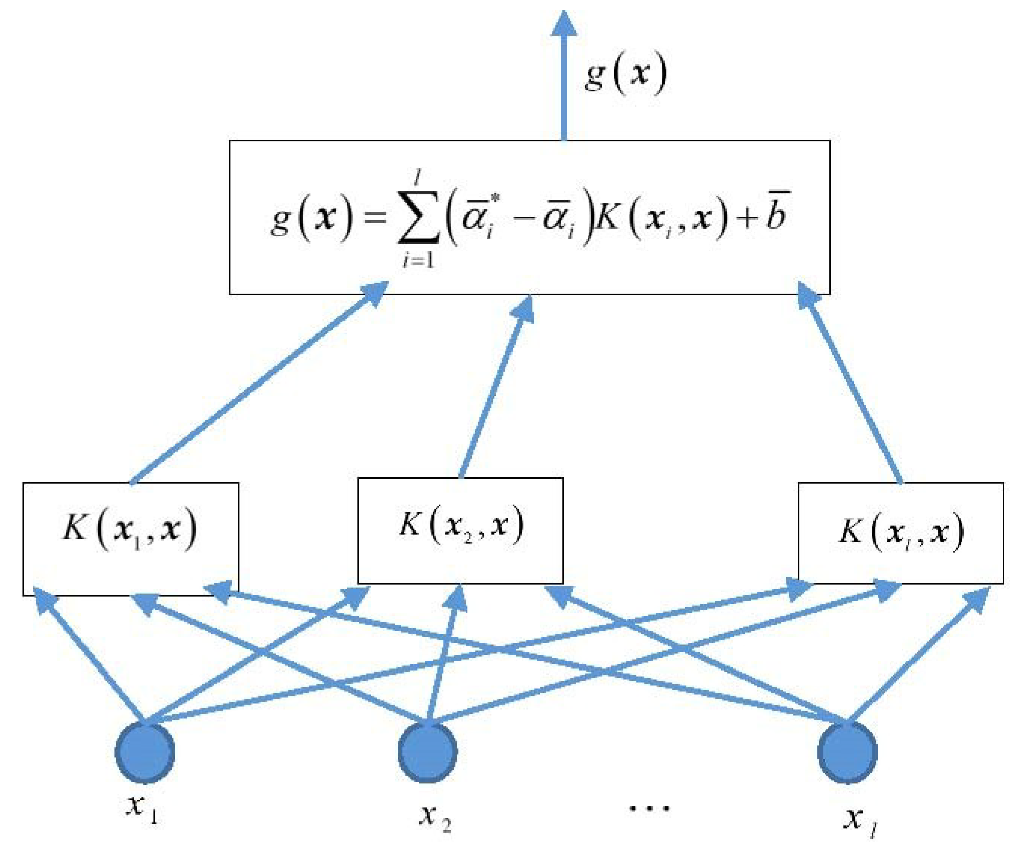
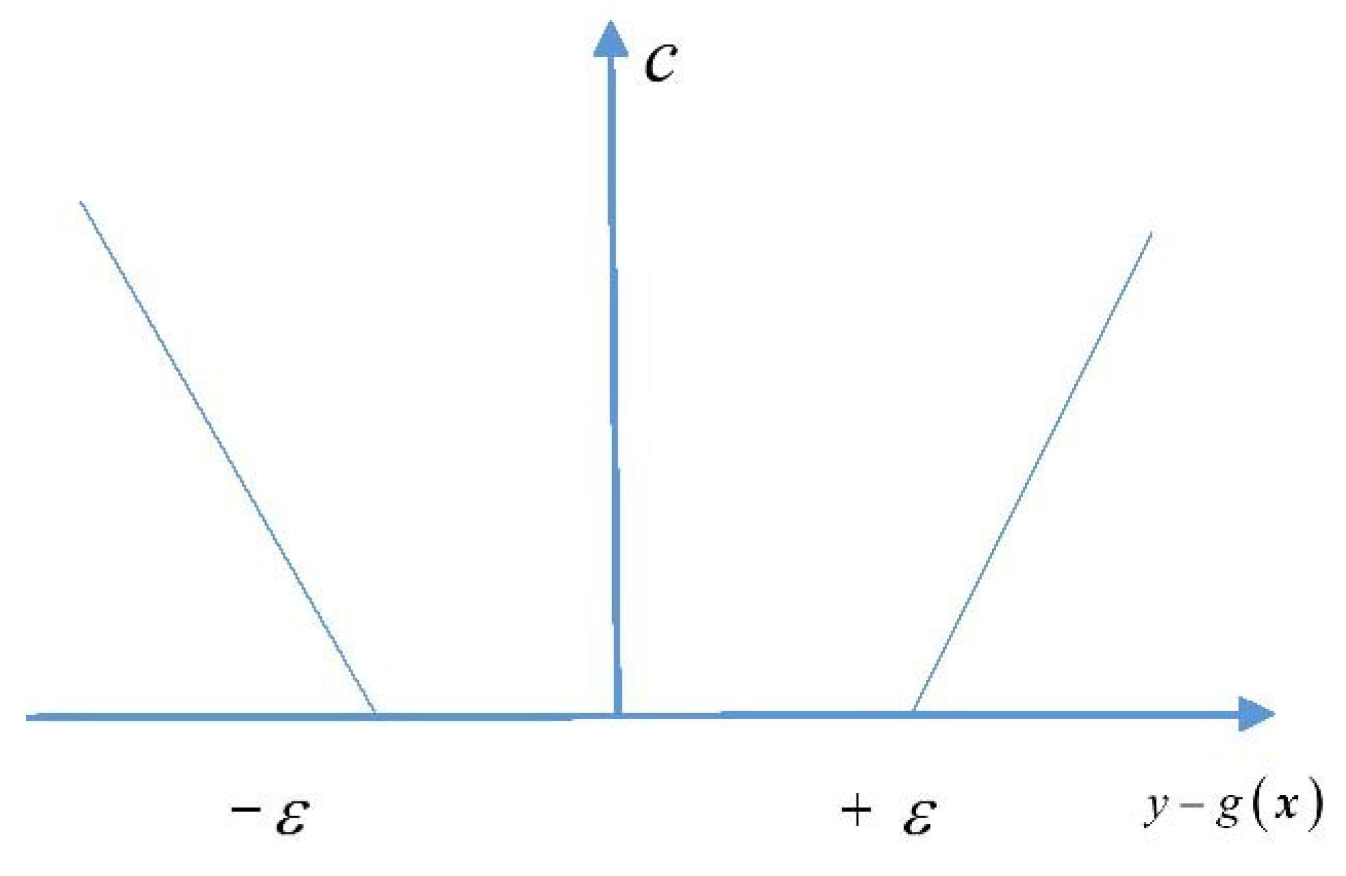
3.1. Support Vector Machine for Regression
3.2. Construction of Mixed Kernel Function
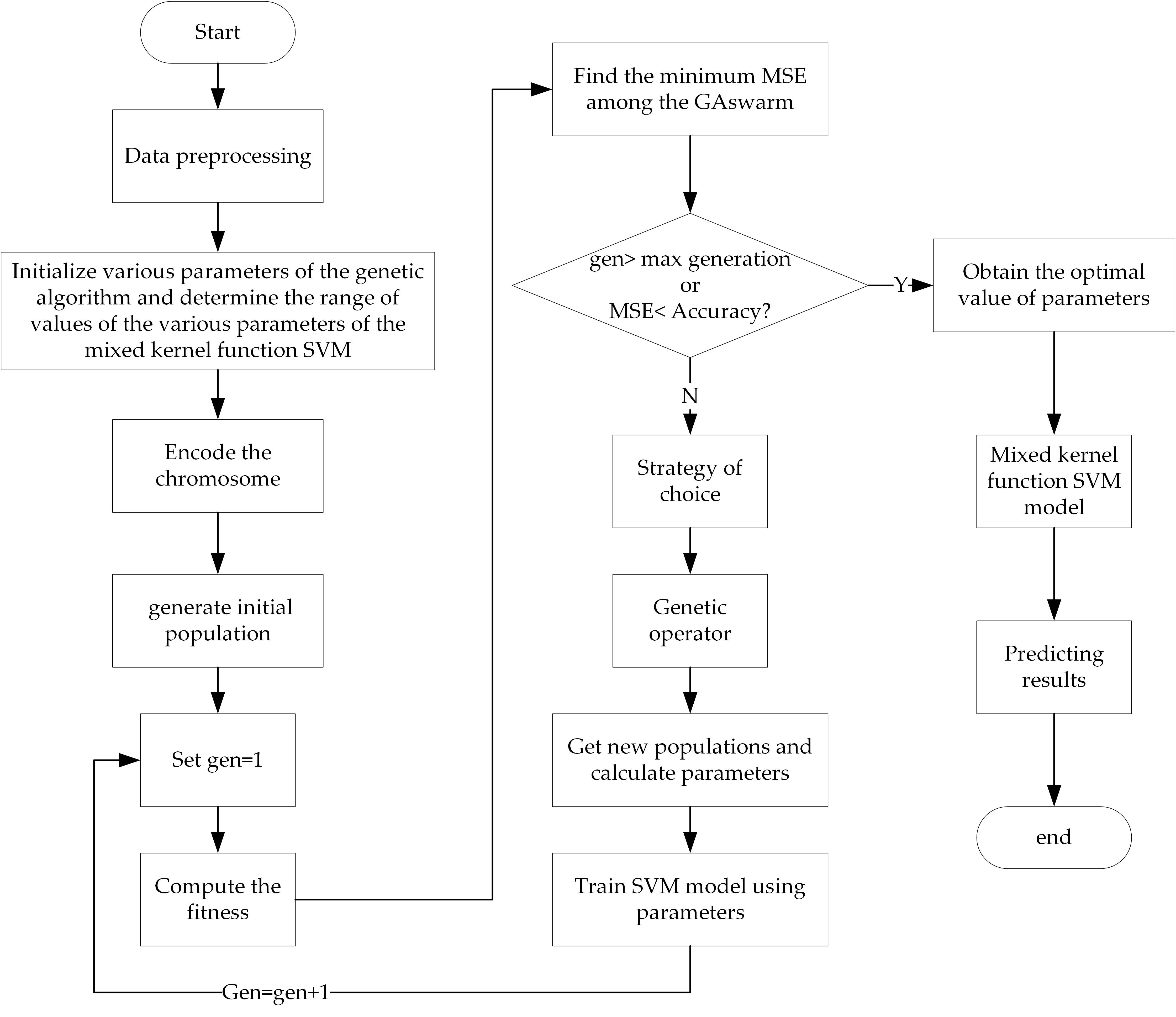
3.3. Parameter Optimization
4. Example Analysis
4.1. Data Samples
- (1)
- , local GDP of the region in which the port of call is located, which can be calculated on the basis of the formula actual amount/100 million yuan;
- (2)
- , changes in port industrial structures, which can calculated according to the percentage occupied by the tertiary industry;
- (3)
- , completeness of the collection and distribution system, which can calculated according to the actual annual throughput of containers per million twenty-foot equivalent units (TEU) at the port of call;
- (4)
- , company’s capacity, which can be calculated according to the actual number of containers/10,000 TEU;
- (5)
- , inland turnaround time of containers, which can be calculated according to the actual number of days;
- (6)
- , seasonal changes in cargo volume, which can be calculated as a percentage;
- (7)
- , quantity of containers handled by the company, which can be calculated according to the actual number of containers/10,000 TEU;
- (8)
- , transport capacity for a single ship, which can be calculated according to the actual number of containers/TEU; and
- (9)
- , full-container-loading rate of the ship, which can be calculated as a percentage.
4.2. Determining the Weight of Influencing Factors
4.3. Prediction of Number of Allocated Containers for One Voyage Using Mixed Kernel SVM
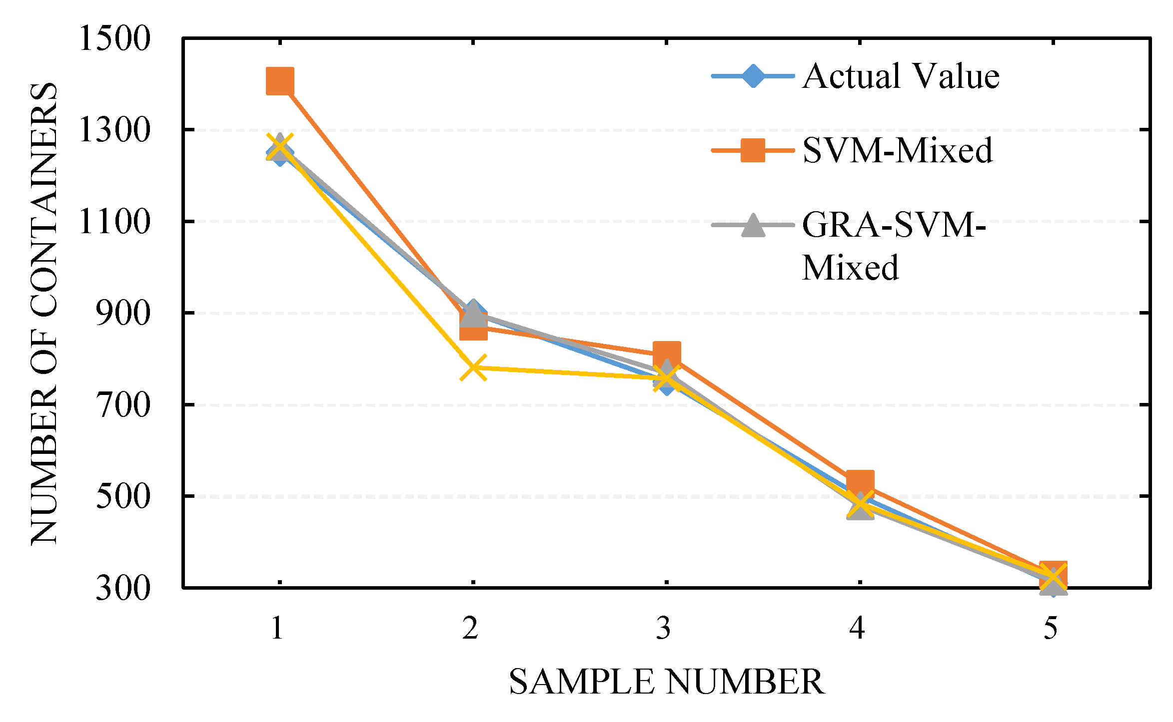
4.4. Simulation Results and Analysis
5. Conclusions
Author Contributions
Funding
Conflicts of Interest
References
- Helo, P.; Paukku, H.; Sairanen, T. Containership cargo profiles, cargo systems, and stowage capacity: Key performance indicators. Marit. Econ. Logist. 2018, 1–21. [Google Scholar] [CrossRef]
- Gosasang, V.; Chandraprakaikul, W.; Kiattisin, S. An application of neural networks for forecasting container throughput at Bangkok port. In Proceedings of the World Congress on Engineering, London, UK, 30 June–2 July 2010; pp. 137–141. [Google Scholar]
- Iris, Ç.; Pacino, D.; Ropke, S.; Larsen, A. Integrated berth allocation and quay crane assignment problem: Set partitioning models and computational results. Transp. Res. Part E Logist. Transp. Rev. 2015, 81, 75–97. [Google Scholar] [CrossRef]
- Jiang, J.; Wang, H.; Yang, Z. Econometric analysis based on the throughput of container and its main influential factors. J. Dalian Marit. Univ. 2007, 1. [Google Scholar] [CrossRef]
- Chou, C. Analysis of container throughput of major ports in Far Eastern region. Marit. Res. J. 2002, 12, 59–71. [Google Scholar] [CrossRef]
- Meersman, H.; Steenssens, C.; Van de Voorde, E. Container Throughput, Port Capacity and Investment; SESO Working Papers 1997020; University of Antwerp, Faculty of Applied Economics: Antwerpen, Belgium, 1997. [Google Scholar]
- Karsten, C.V.; Ropke, S.; Pisinger, D. Simultaneous optimization of container ship sailing speed and container routing with transit time restrictions. Transp. Sci. 2018, 52, 769–787. [Google Scholar] [CrossRef]
- Weiying, Z.; Yan, L.; Zhuoshang, J. A Forecast Model of the Number of Containers for Containership Voyage Based on SVM. Shipbuild. China 2006, 47, 101–107. [Google Scholar]
- Li, S. A forecast method of safety container possession based on neural network. Navig. China 2002, 3, 56–60. [Google Scholar]
- Grudnitski, G.; Osburn, L. Forecasting S&P and gold futures prices: An application of neural networks. J. Futures Mark. 1993, 13, 631–643. [Google Scholar] [CrossRef]
- White, H. Connectionist nonparametric regression: Multilayer feedforward networks can learn arbitrary mappings. Neural Netw. 1990, 3, 535–549. [Google Scholar] [CrossRef]
- Chakraborty, K.; Mehrotra, K.; Mohan, C.K.; Ranka, S. Forecasting the behavior of multivariate time series using neural networks. Neural Netw. 1992, 5, 961–970. [Google Scholar] [CrossRef]
- Lapedes, A.; Farber, R. Nonlinear signal processing using neural networks: Prediction and system modelling. In Proceedings of the IEEE International Conference on Neural Networks, San Diego, CA, USA, 21 June 1987. [Google Scholar]
- Yu, J.; Tang, G.; Song, X.; Yu, X.; Qi, Y.; Li, D.; Zhang, Y. Ship arrival prediction and its value on daily container terminal operation. Ocean Eng. 2018, 157, 73–86. [Google Scholar] [CrossRef]
- Hsu, C.; Huang, Y.; Wong, K.I. A Grey hybrid model with industry share for the forecasting of cargo volumes and dynamic industrial changes. Transp. Lett. 2018, 1–12. [Google Scholar] [CrossRef]
- Vapnik, V.N. An overview of statistical learning theory. IEEE Trans. Neural Netw. 1999, 10, 988–999. [Google Scholar] [CrossRef] [PubMed]
- Cortes, C.; Vapnik, V. Support-vector networks. Mach. Learn. 1995, 20, 273–297. [Google Scholar] [CrossRef]
- Müller, K.R.; Smola, A.J.; Rätsch, G.; Schölkopf, B.; Kohlmorgen, J.; Vapnik, V. Predicting time series with support vector machines. In Proceedings of the Artificial Neural Networks—ICANN’97, Lausanne, Switzerland, 8–10 October 1997; Springer: Berlin/Heidelberg, Germany, 1997; pp. 999–1004. [Google Scholar] [CrossRef]
- Gunn, S.R. Support vector machines for classification and regression. ISIS Tech. Rep. 1998, 14, 5–16. [Google Scholar]
- Joachims, T. Making Large-Scale SVM Learning Practical. Technical Report, SFB 475. 1998, Volume 28. Available online: http://hdl.handle.net/10419/77178 (accessed on 15 June 1998).
- Smits, G.F.; Jordaan, E.M. Improved SVM regression using mixtures of kernels. In Proceedings of the 2002 International Joint Conference on Neural Networks, Honolulu, HI, USA, 12–17 May 2002; pp. 2785–2790. [Google Scholar] [CrossRef]
- Jebara, T. Multi-task feature and kernel selection for SVMs. In Proceedings of the Twenty-First International Conference on Machine Learning, Banff, AB, Canada, 4–8 July 2004; pp. 329–337. [Google Scholar] [CrossRef]
- Tsang, I.W.; Kwok, J.T.; Cheung, P. Core vector machines: Fast SVM training on very large data sets. J. Mach. Learn. Res. 2005, 6, 363–392. [Google Scholar]
- Lu, Y.L.; Lei, L.I.; Zhou, M.M.; Tian, G.L. A new fuzzy support vector machine based on mixed kernel function. In Proceedings of the 2009 International Conference on Machine Learning and Cybernetics, Baoding, China, 12–15 July 2009; pp. 526–531. [Google Scholar] [CrossRef]
- Xie, G.; Wang, S.; Zhao, Y.; Lai, K.K. Hybrid approaches based on LSSVR model for container throughput forecasting: A comparative study. Appl. Soft Comput. 2013, 13, 2232–2241. [Google Scholar] [CrossRef]
- Deng, J.L. Introduction to Grey System Theory. J. Grey Syst. 1989, 1, 1–24. [Google Scholar]
- Al-Douri, Y.; Hamodi, H.; Lundberg, J. Time Series Forecasting Using a Two-Level Multi-Objective Genetic Algorithm: A Case Study of Maintenance Cost Data for Tunnel Fans. Algorithms 2018, 11, 123. [Google Scholar] [CrossRef]
- Weiwei, W. Time series prediction based on SVM and GA. In Proceedings of the 2007 8th International Conference on Electronic Measurement and Instruments, Xi’an, China, 16–18 August 2007; pp. 307–310. [Google Scholar] [CrossRef]
- Yin, Y.; Cui, H.; Hong, M.; Zhao, D. Prediction of the vertical vibration of ship hull based on grey relational analysis and SVM method. J. Mar. Sci. Technol. 2015, 20, 467–474. [Google Scholar] [CrossRef]
- Kuo, Y.; Yang, T.; Huang, G. The use of grey relational analysis in solving multiple attribute decision-making problems. Comput. Ind. Eng. 2008, 55, 80–93. [Google Scholar] [CrossRef]
- Tosun, N. Determination of optimum parameters for multi-performance characteristics in drilling by using grey relational analysis. Int. J. Adv. Manuf. Technol. 2006, 28, 450–455. [Google Scholar] [CrossRef]
- Shen, M.X.; Xue, X.F.; Zhang, X.S. Determination of Discrimination Coefficient in Grey Incidence Analysis. J. Air Force Eng. Univ. 2003, 4, 68–70. [Google Scholar]
- Yao, X.; Zhang, L.; Cheng, M.; Luan, J.; Pang, F. Prediction of noise in a ship’s superstructure cabins based on SVM method. J. Vib. Shock 2009, 7. [Google Scholar] [CrossRef]
- Huang, C.; Chen, M.; Wang, C. Credit scoring with a data mining approach based on support vector machines. Expert Syst. Appl. 2007, 33, 847–856. [Google Scholar] [CrossRef]
- Duan, K.; Keerthi, S.S.; Poo, A.N. Evaluation of simple performance measures for tuning SVM hyperparameters. Neurocomputing 2003, 51, 41–59. [Google Scholar] [CrossRef]
- Van der Schaar, M.; Delory, E.; André, M. Classification of sperm whale clicks (Physeter Macrocephalus) with Gaussian-Kernel-based networks. Algorithms 2009, 2, 1232–1247. [Google Scholar] [CrossRef]
- Luo, W.; Cong, H. Control for Ship Course-Keeping Using Optimized Support Vector Machines. Algorithms 2016, 9, 52. [Google Scholar] [CrossRef]
- Wei, Y.; Yue, Y. Research on Fault Diagnosis of a Marine Fuel System Based on the SaDE-ELM Algorithm. Algorithms 2018, 11, 82. [Google Scholar] [CrossRef]
- Bian, Y.; Yang, M.; Fan, X.; Liu, Y. A Fire Detection Algorithm Based on Tchebichef Moment Invariants and PSO-SVM. Algorithms 2018, 11, 79. [Google Scholar] [CrossRef]
- Cherkassky, V.; Ma, Y. Practical selection of SVM parameters and noise estimation for SVM regression. Neural Netw. 2004, 17, 113–126. [Google Scholar] [CrossRef]
- Aiqin, H.; Yong, W. Pressure model of control valve based on LS-SVM with the fruit fly algorithm. Algorithms 2014, 7, 363–375. [Google Scholar] [CrossRef]
- Du, J.; Liu, Y.; Yu, Y.; Yan, W. A prediction of precipitation data based on support vector machine and particle swarm optimization (PSO-SVM) algorithms. Algorithms 2017, 10, 57. [Google Scholar] [CrossRef]
- Wang, R.; Tan, C.; Xu, J.; Wang, Z.; Jin, J.; Man, Y. Pressure Control for a Hydraulic Cylinder Based on a Self-Tuning PID Controller Optimized by a Hybrid Optimization Algorithm. Algorithms 2017, 10, 19. [Google Scholar] [CrossRef]
- Liu, D.; Niu, D.; Wang, H.; Fan, L. Short-term wind speed forecasting using wavelet transform and support vector machines optimized by genetic algorithm. Renew. Energy 2014, 62, 592–597. [Google Scholar] [CrossRef]
- Shevade, S.K.; Keerthi, S.S.; Bhattacharyya, C.; Murthy, K.R.K. Improvements to the SMO algorithm for SVM regression. IEEE Trans. Neural Netw. 2000, 11, 1188–1193. [Google Scholar] [CrossRef] [PubMed]
- Holland, J.H. Adaptation in Natural and Artificial Systems: An Introductory Analysis with Applications to Biology, Control, and Artificial Intelligence; MIT Press: Cambridge, MA, USA, 1992. [Google Scholar]


| No. | ||||||||||
|---|---|---|---|---|---|---|---|---|---|---|
| 1 | 2395 | 75 | 2461 | 10.3 | 11 | 20 | 21 | 5200 | 77 | 1100 |
| 2 | 27,689 | 66 | 776 | 85 | 38 | 10 | 170 | 1700 | 85 | 279 |
| 3 | 29,960 | 77 | 2521 | 102.3 | 10 | 15 | 230 | 4700 | 69 | 1739 |
| 4 | 29,841 | 82 | 4123 | 162 | 49 | 13 | 201 | 3410 | 64 | 177 |
| 5 | 13,562 | 63 | 2357 | 68.9 | 39 | 20 | 150 | 1200 | 73 | 110 |
| 6 | 17,369 | 59 | 2037 | 60.3 | 22 | 26 | 120 | 800 | 62 | 205 |
| 7 | 14,650 | 71 | 1521 | 59 | 13 | 29 | 147 | 2800 | 73 | 347 |
| 8 | 30,550 | 58 | 798 | 47.7 | 26 | 15 | 128 | 3600 | 88 | 561 |
| 9 | 25,103 | 54 | 567 | 110.3 | 13 | 10 | 235 | 2000 | 65 | 850 |
| 10 | 14,650 | 65 | 668 | 85.6 | 25 | 12 | 164 | 2590 | 86 | 496 |
| 11 | 14,023 | 49 | 732 | 77.7 | 16 | 30 | 139 | 2810 | 59 | 594 |
| 12 | 19,776 | 67 | 651 | 56 | 30 | 21 | 98 | 1400 | 71 | 350 |
| Factors | Relevance | Factors | Relevance | Factors | Relevance |
|---|---|---|---|---|---|
| 0.1669 | 0.1773 | 0.1770 | |||
| 0.6672 | 0.3998 | 0.8345 | |||
| 0.7084 | 0.6206 | 0.6232 |
| Factors | Weight | Factors | Weight | Factors | Weight |
|---|---|---|---|---|---|
| 0.038 | 0.041 | 0.040 | |||
| 0.153 | 0.091 | 0.191 | |||
| 0.162 | 0.142 | 0.142 |
| No. | ||||||||||
|---|---|---|---|---|---|---|---|---|---|---|
| 1 | 4365 | 76 | 1596 | 24 | 13 | 18 | 43 | 5400 | 72 | 1250 |
| 2 | 23,560 | 69 | 882 | 87 | 29 | 12 | 185 | 1900 | 83 | 900 |
| 3 | 9841 | 81 | 2143 | 112 | 12 | 17 | 251 | 4580 | 70 | 750 |
| 4 | 25,590 | 74 | 4265 | 159 | 50 | 14 | 211 | 3390 | 66 | 500 |
| 5 | 18,763 | 62 | 1983 | 73 | 41 | 21 | 163 | 1080 | 74 | 310 |
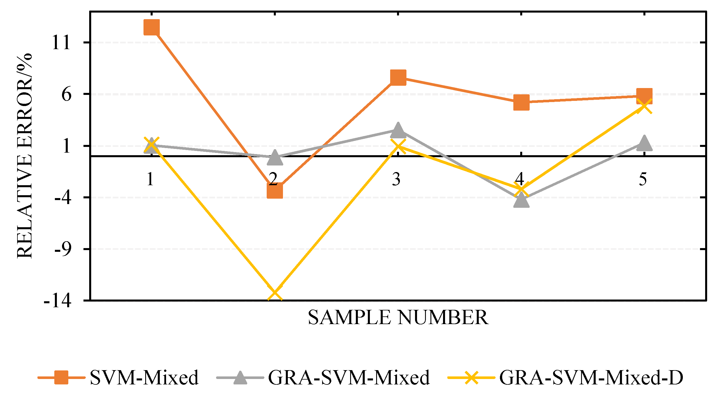
| No. | Actual | SVM-Mixed | GRA-SVM-Mixed | GRA-SVM-Mixed-D | |||
|---|---|---|---|---|---|---|---|
| Predictive | Relative Error | Predictive | Relative Error | Predictive | Relative Error | ||
| 1 | 1250 | 1406 | 12.48 | 1263 | 1.04 | 1264 | 1.12 |
| 2 | 900 | 870 | −3.33 | 899 | −0.11 | 781 | −13.22 |
| 3 | 750 | 807 | 7.60 | 769 | 2.53 | 757 | 0.93 |
| 4 | 500 | 526 | 5.20 | 479 | −4.20 | 484 | −3.20 |
| 5 | 310 | 328 | 5.81 | 314 | 1.29 | 325 | 4.84 |
| MSE | 5897 | 197.6 | 2977.4 | ||||
| 6.88 | 1.83 | 4.66 | |||||
| 0.9908 | 0.9993 | 0.9877 | |||||
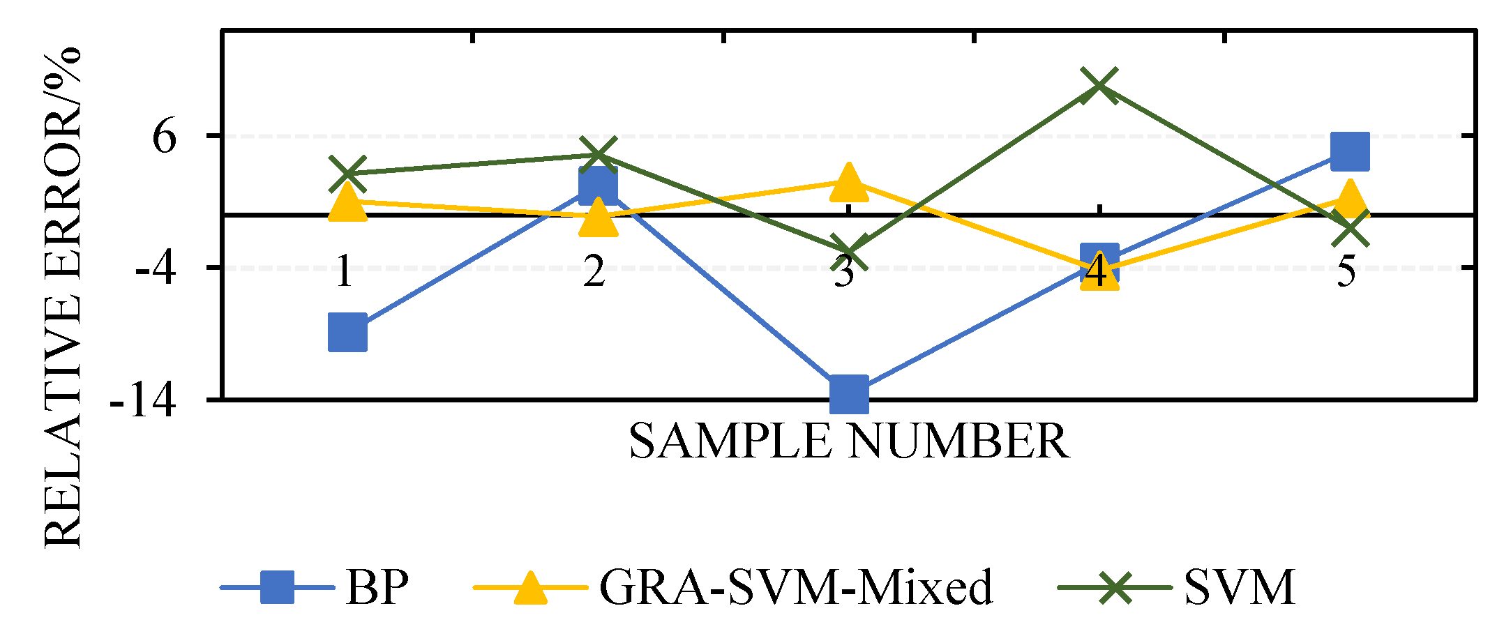
| No. | Relative Error | ||
|---|---|---|---|
| BP | SVM | GRA-SVM-Mixed | |
| 1 | −8.88 | 3.12 | 1.04 |
| 2 | 2.22 | 4.56 | −0.11 |
| 3 | −13.6 | −2.80 | 2.53 |
| 4 | −3.6 | 9.80 | −4.20 |
| 5 | 4.84 | −0.97 | 1.29 |
| MES | 4734.8 | 1210.6 | 197.6 |
| 0.9883 | 0.9969 | 0.9993 | |
| t/s | 57.63 | 45.61 | 27.53 |
© 2018 by the authors. Licensee MDPI, Basel, Switzerland. This article is an open access article distributed under the terms and conditions of the Creative Commons Attribution (CC BY) license (http://creativecommons.org/licenses/by/4.0/).
Share and Cite
Wang, Y.; Shi, G.; Sun, X. A Forecast Model of the Number of Containers for Containership Voyage. Algorithms 2018, 11, 193. https://doi.org/10.3390/a11120193
Wang Y, Shi G, Sun X. A Forecast Model of the Number of Containers for Containership Voyage. Algorithms. 2018; 11(12):193. https://doi.org/10.3390/a11120193
Chicago/Turabian StyleWang, Yuchuang, Guoyou Shi, and Xiaotong Sun. 2018. "A Forecast Model of the Number of Containers for Containership Voyage" Algorithms 11, no. 12: 193. https://doi.org/10.3390/a11120193
APA StyleWang, Y., Shi, G., & Sun, X. (2018). A Forecast Model of the Number of Containers for Containership Voyage. Algorithms, 11(12), 193. https://doi.org/10.3390/a11120193