An Algorithm for Interval-Valued Intuitionistic Fuzzy Preference Relations in Group Decision Making Based on Acceptability Measurement and Priority Weight Determination

Abstract

Group decision making with intuitionistic fuzzy preference information contains two key issues: acceptability measurement and priority weight determination. In this paper, we investigate the above two issues with respect to multiplicative interval-valued intuitionistic fuzzy preference relation (IVIFPR). Firstly, a consistency index is defined to measure the multiplicative consistency degree of IVIFPR and an optimization model is established to improve the consistency degree of IVIFPR to an acceptable one. Next, in terms of priority weight determination, an error-analysis-based extension method is proposed to obtain priority weight vector from the acceptable IVIFPR. For GDM problems, decision makers’ weights are derived by the proposed multiplicative consistency index. Subsequently, the collective IVIFPR is obtained by using an interval-valued intuitionistic fuzzy (IVIF) weighted averaging operator. Finally, a step-by step algorithm for GDM with IVIFPRs is given, and an example of enterprise innovation partner selection is analyzed, and comparative analyses with existing approaches are performed to demonstrate that the proposed algorithm is both effective and practical in dealing with GDM problems.

1. Introduction

In Group decision making (GDM), various decision makers (DMs or experts) would be employed to express their preferences via pairwise comparison over decision alternatives. Two classical preference relations consist of fuzzy preference relations (FPRs) [1,2] and multiplicative preference relations (MPRs) [3,4], in which the elements are described by exact numerical values. However, due to the uncertainty and complex information granularity, DMs may have difficulty in providing pairwise comparison judgments on alternatives with crisp numerical values. To address this issue, the intuitionistic fuzzy preference relation (IFPR) [5,6], interval-valued fuzzy preference relation (IVFPR) [7,8] and interval-valued intuitionistic fuzzy (IVIF) preference relation (IVIFPR) [9,10] appear one after another. Particularly, the elements in an IVIFPR consist of IVIF values (IVIFVs), where both the membership degree and non-membership degree are intervals. Therefore, IVIFPR can flexibly seize such uncertainty and vagueness information in decision making. In recent decades, IVIFPR has been widely used to solve different GDM problems, such as the supplier selection [11], the virtual enterprise partner selection [12], the transport service provider selection [13], the air traffic protection aircraft [14] and so on.

The consistency degree of comparison matrices directly affects the final decision result. For GDM problems, the consistent IVIFPRs provided by DMs refer to certain transitivity property, which can ensure that DMs’ judgments contain no contradiction in some sense. Therefore, it is natural that the consistency of IVIFPRs should be measured and improved in GDM problems. To date, a host of studies have been devoted to discussing this issue. For instance, Xu and Chen [15] first proposed the concept of the consistent interval-valued intuitionistic judgment matrix. Subsequently, Xu and Cai [16,17] introduced some definitions on multiplicative and additive consistency in incomplete IVIFPR and determined the missing elements in an IVIFPR while only knowing its off-diagonal elements. Inspired by the multiplicative transitivity of an IVIFPR, Liao et al. [18] proposed a multiplicative consistency concept to an IVIFPR, which was applied to adjust or repair an inconsistent IVIFPR through using some iterative algorithms. These achievements directly investigated the multiplicative transitivity property of an IVIFPR. In contrast, Wan et al. [12] indirectly examined the multiplicative consistency of an IVIFPR by inducing two special IFRP matrices from an IVIFPRs. Subsequently, with the same idea, Wan et al. [9,10] defined the additive consistency of an IVIFPR by generating two special IVFPRs and extracting two consistent IFPR from an IVIFPR, respectively. Chu et al. [11] put forward a new definition on the additive consistency of an IVIFPR by dividing an IVIFPR into four preference relations. Meng et al. [19] built 0–1 mixed programming models to judge the multiplicative consistency of IVIFPRs, and developed a multiplicative consistency and consensus based algorithm to GDM with IVIFPRs. Mukhametzyanov et al. [20] used statistical approach and presented a sensitivity analysis model to discuss the result for consistency evaluation of decision making.

Since the priority weights can be utilized to rank alternatives, it is an important issue to determine the priority weights for GDM problems based on preference relations [21]. Due to the complex operations on IVIFVs, research paper on determining priority weights from IVIFPRs are very scarce. For example, Xu and Chen [15] developed an approach to GDM with IVIFPR by the ordered weighted and hybrid aggregation operators. Xu and Yager [22] proposed a similarity measure between IFPRs and extended it to IVIFPRs. Wu and Chiclana [23] introduced a new attitudinal expected score function for interval-valued intuitionistic fuzzy numbers. Yue [24] presented a geometric approach for ranking IVIFVs. Wan et al. [9] and Chu et al. [11] constructed optimization models to derive priority weights by using the associated matrices of IVFPR or IFPR form an IVIFPR. Zhou et al. [25] developed a logarithm least optimal model to derive interval priority weights of IFPR and then proposed a two-stage resolution process for GDM with IVIFPRs.

The achievements, as mentioned, have significantly advanced the research on GDM with IVIFPRs. Nevertheless, there still exist some drawbacks, as stated below:

(1)

While checking the consistency degree of a given IVIFPR, existing research [17,18] has proposed the definitions of a consistent IVIFPR, which can be used to judge whether an IVIFPR is consistent or not. However, none of them can measure the consistency degree of an inconsistent IVIFPR. Other literature (References [10,12,19]) has also defined the consistency of an IVIFPR through extracting associated preference matrices from original IVIFPR, which cannot fully attach the initial preference information and needs to be constructed by the numerous computational efforts. Therefore, it is necessary to find a convenient solution to check the consistency degrees of IVIFPRs.

(2)

When a given IVIFPR is unacceptably consistent, only Liao et al. [18] and Wan et al. [12] proposed some iterative algorithms to improve its consistency degree. Nevertheless, it may be to repeat these algorithms several times to repair this unacceptably consistent IVIFPR until the acceptable consistency is achieved. This is time consuming and requires heavy workload. Furthermore, it is unknown how much of the repaired IVIFPR reserves preference information for the initial IVIFPR.

(3)

As for the determination of priority weights of alternatives for IVIFPRs, the existing studies [15,22,24] have directly adopted the formulas to rank the alternatives. However, such formulas are only applicable to consistent IVIFPRs and would be ineffective for inconsistent IVIFPRs. Other methods (References [9,11,25]) have established some optimizing or linear models to determine the priority weights, noting that these optimizing or linear models only minimize the deviation between the associated matrices form original IVIFPR and the converted consistent one to the most extent. However, for an extremely unacceptable consistent IVIFPR, the priority weights obtained by such models are unreasonable and cannot be accepted in decision making.

To fill the literature review gap, this paper concentrates on developing a novel algorithm for IVIFPRs in GDM problems based on acceptability measurement and priority weight determination. Firstly, following the work of Liao et al. [18], the multiplicative consistency index of an IVIFPR is defined considering DM’s risk attitude. Then an optimization model is built to improve the consistency degree of an unacceptable multiplicative consistent IVIFPR and obtain an acceptable multiplicative consistent one. With regard to the determination of priority weights of an IVIFPR, inspired by Xu [26], an error-analysis-based extension method is proposed. In GDM problems, DMs’ weights are generated by the defined multiplicative consistency index. Subsequently, the collective IVIFPR is obtained through using an IVIF weighted averaging operator. Finally, a step-by-step algorithm for GDM with IVIFPRs is developed. An example of enterprise innovation partner selection is analyzed to demonstrate its practicability and effectiveness. Some significant features of this paper are outlined as follows:

(1)

Liao et al. [18] defined the multiplicative consistency of IVIFPR to adjust or repair the inconsistent IVIFPRs. The consistent degree of an inconsistent IVIFPR cannot be measured by [18]. To measure the consistency degree of an IVIFPR, according to the multiplicative consistency definition in Reference [18], this paper proposes a new concept of multiplicative consistency index of an IVIFPR by considering various decision-making principles (i.e., the majority and minority principles). A notable feature is that multiplicative consistency index of an IVIFPR can be directly obtained from original IVIFPR without any transformation via Wan et al. [12]. Therefore, the definition of multiplicative consistency index of an IVIFPR is easy to operate.

(2)

An optimization model is directly established to repair and improve the consistency of IVIFPR. Compared with iterative algorithms proposed in References [12,18], the proposed model can not only rapidly obtain an acceptable consistent IVIFPR from the initial IVIFPR, but also enables the obtained IVIFPR to retain as much as possible the preference information hidden in the initial IVIFPR.

(3)

An error-analysis-based extension method is developed to derive IVIF priority weights from the acceptable consistent IVIFPR. Compared with some optimization models proposed in References [9,11,12], the extension method can simplify computation and save time. Moreover, in GDM problems, DMs’ weights are generated by using the proposed multiplicative consistency index of an IVIFPR, which is objective and reasonable to some extent.

The remainder of this paper is organized as follows. In Section 2, some basic related concepts on preference relations are reviewed. In Section 3, the multiplicative consistency index of IVIFPR is defined, and then an optimization model is built to obtain acceptable consistency of an IVIFPR. In Section 4, an error-analysis-based method is extended to determine IVIF priority weights. In Section 5, GDM problems with IVIFPRs are considered, then DMs’ weights are derived, and an algorithm for GDM with IVIFPRs is developed. In Section 6, a practical example of enterprise innovation partner selection is presented to demonstrate the efficiency and applicability of the proposed algorithm. Section 7 concludes the study.

2. Preliminaries

In this section, some associated definitions on preference relations are reviewed, and the error propagation formula is also discussed.

2.1. Some Associated Definitions on Preference Relations

Definition 1.

[27] An IVFPR $R$ on the alternative set $X=\left\{x_1,x_2,\dots ,x_n\right\}$ is presented by an interval-valued fuzzy judgment matrix $R={\left(r_{ij}\right)}_{n\times n}\subset X\times X$ with $r_{ij}=\left[{\underset{\_}{r}}_{ij},{\overline{r}}_{ij}\right]$, where the preference degree to which alternative $x_i$ over $x_j$ is between ${\underset{\_}{r}}_{ij}$ and ${\overline{r}}_{ij}$. Moreover, ${\underset{\_}{r}}_{ij}$ and ${\overline{r}}_{ij}$ fulfill the following conditions:

$$0\le {\underset{\_}{r}}_{ij}\le {\overline{r}}_{ij}\le 1,{\underset{\_}{r}}_{ij}+{\overline{r}}_{ji}=1,{\underset{\_}{r}}_{ii}={\overline{r}}_{ii}=0.5\mathrm{for}\mathrm{all}i,j=1,2,\dots ,n.$$

Definition 2.

[28] Let $X=\left\{x_1,x_2,\dots ,x_n\right\}$ be a non-empty alternative set. An IVIF set $\tilde{A}$ in $X$ is denoted by $\tilde{A}=\left\{X,{\mu }_{\tilde{A}}\left(x\right),v_{\tilde{A}}\left(x\right)|x\in X\right\}$, where ${\mu }_{\tilde{A}}\left(x\right)=\left[{\underset{\_}{\mu }}_{\tilde{A}}\left(x\right),{\overline{\mu }}_{\tilde{A}}\left(x\right)]\subseteq [0,1\right]$, and $v_{\tilde{A}}\left(x\right)=\left[{\underset{\_}{v}}_{\tilde{A}}\left(x\right),{\overline{v}}_{\tilde{A}}\left(x\right)]\subseteq [0,1\right]$. ${\mu }_{\tilde{A}}\left(x\right)$ and $v_{\tilde{A}}\left(x\right)$ are interval values, indicating that the membership degree and non-membership degree of element X to IVIFV $\tilde{A}$, respectively, meeting ${\overline{\mu }}_{\tilde{A}}\left(x\right)+{\overline{v}}_{\tilde{A}}\left(x\right)\le 1$ for any $x\in X$. Therefore, the IVIFV $\tilde{A}$ can be expressed as $\tilde{A}=\left\{\left(X,{\underset{\_}{[\mu }}_{\tilde{A}}\left(x\right),{\overline{\mu }}_{\tilde{A}}\left(x\right)],[{\underset{\_}{v}}_{\tilde{A}}\left(x\right),{\overline{v}}_{\tilde{A}}\left(x\right)\right])|x\in X\right\}$.

Similarly,${\tilde{\pi }}_{\tilde{A}}\left(x\right)=\left[{\underset{\_}{\pi }}_{\tilde{A}}\left(x\right),{\overline{\pi }}_{\tilde{A}}\left(x\right)\right]$is named the interval hesitancy preference degree for any$x\in X$, where${\underset{\_}{\pi }}_{\tilde{A}}\left(x\right)=1-{\overline{\mu }}_{\tilde{A}}\left(x\right)-{\overline{v}}_{\tilde{A}}\left(x\right)$and${\overline{\pi }}_{\tilde{A}}\left(x\right)=1-{\underset{\_}{\mu }}_{\tilde{A}}\left(x\right)-{\underset{\_}{v}}_{\tilde{A}}\left(x\right)$.

The pair$\theta =\left(\left[\underset{\_}{\mu },\overline{\mu }],[\underset{\_}{v},\overline{v}\right]\right)$is call an interval-valued intuitionistic fuzzy value (IVIFV) [29], where $\left[\underset{\_}{\mu },\overline{\mu }]\subseteq [0,1\right]$ and $\left[\underset{\_}{v},\overline{v}]\subseteq [0,1\right]$. Xu and Chen [15] proposed the concepts of the score function and accuracy function, which is one of the feasible methods to rank IVIFV.

Definition 3.

[15] For an IVIFV $\theta =\left(\left[\underset{\_}{\mu },\overline{\mu }],[\underset{\_}{v},\overline{v}\right]\right)$, the score function $S\left(\theta \right)$ is

$$S\left(\theta \right)=\frac{1}{2}\left(\underset{\_}{\mu }-\underset{\_}{v}+\overline{\mu }-\overline{v}\right)$$

(1)

and accuracy function $H\left(\theta \right)$ is

$$H\left(\theta \right)=\frac{1}{2}\left(\underset{\_}{\mu }+\overline{\mu }+\underset{\_}{v}+\overline{v}\right)$$

(2)

For any two IVIFVs${\theta }_1=\left(\left[{\underset{\_}{\mu }}_1,{\overline{\mu }}_1],[{\underset{\_}{v}}_1,{\overline{v}}_1\right]\right)$and${\theta }_2=\left(\left[{\underset{\_}{\mu }}_2,{\overline{\mu }}_2],[{\underset{\_}{v}}_2,{\overline{v}}_2\right]\right)$

• If$S\left({\theta }_1\right)>S\left({\theta }_2\right)$, then${\theta }_1>{\theta }_2$.
• If$S\left({\theta }_1\right)=S\left({\theta }_2\right)$, then
• If$H\left({\theta }_1\right)>H\left({\theta }_2\right)$, then${\theta }_1>{\theta }_2$.
• If$H\left({\theta }_1\right)<H\left({\theta }_2\right)$, then${\theta }_1<{\theta }_2$.
• If$H\left({\theta }_1\right)=H\left({\theta }_2\right)$, then${\theta }_1={\theta }_2$.

Definition 4.

[15] Let $X=\left\{x_1,x_2,\dots ,x_n\right\}$ be a non-empty alternative set. An IVIFPR $\tilde{R}$ on the set X is denoted by $\tilde{R}={({\tilde{r}}_{ij})}_{n\times n}\subset Z\times Z$ with ${\tilde{r}}_{ij}=\left(\left[{\underset{\_}{\mu }}_{ij},{\overline{\mu }}_{ij}],[{\underset{\_}{v}}_{ij},{\overline{v}}_{ij}\right]\right)$, where $\left[{\underset{\_}{\mu }}_{ij},{\overline{\mu }}_{ij}\right]$ and $\left[{\underset{\_}{v}}_{ij},{\overline{v}}_{ij}\right]$ are the preference degree and no-preference degree to which alternative $x_i$ over $x_j$, and ${\tilde{\pi }}_{ij}=\left[1-{\overline{\mu }}_{ij}\left(x\right)-{\overline{v}}_{ij}\left(x\right),1-{\underset{\_}{\mu }}_{ij}\left(x\right)-{\underset{\_}{v}}_{ij}\left(x\right)\right]$ is represented as interval hesitancy preference degree to which alternative $x_i$ over $x_j$. Moreover, $\left[{\underset{\_}{\mu }}_{ij},{\overline{\mu }}_{ij}\right]$ and $\left[{\underset{\_}{v}}_{ij},{\overline{v}}_{ij}\right]$ fulfill the conditions as follow:

$$\begin{array}{c}\left[{\underset{\_}{\mu }}_{ij},{\overline{\mu }}_{ij}\right]\subseteq \left[0,1\right],\left[{\underset{\_}{v}}_{ij},{\overline{v}}_{ij}\right]\subseteq \left[0,1\right],\left[{\underset{\_}{\mu }}_{ii},{\overline{\mu }}_{ii}\right]=\left[{\underset{\_}{v}}_{ii},{\overline{v}}_{ii}\right]=\left[0.5,0.5\right], 0\le {\overline{\mu }}_{ij}+{\overline{v}}_{ij}\le 1\\ \left[{\underset{\_}{\mu }}_{ij},{\overline{\mu }}_{ij}\right]=\left[{\underset{\_}{v}}_{ji},{\overline{v}}_{ji}\right], \left[{\underset{\_}{v}}_{ij},{\overline{v}}_{ij}\right]=\left[{\underset{\_}{\mu }}_{ji},{\overline{\mu }}_{ji}\right]\mathrm{for}\mathrm{all}i,j=1,2,\dots ,n.\end{array}$$

Remark 1.

Owing to the increasingly sophisticated decision-making environment and the vagueness of the human mind, it is hard to provide certain preferences on the pairwise comparison of alternatives regarding $\left(\left[0,1\right],\left[0,1\right]\right)$ or $\left(\left[1,1\right],\left[1,1\right]\right)$. Meanwhile, decision makers are usually experts in the decision-making issues in which they participate and the complete stubbornness rarely occurs. Therefore, the preference value$\left(\left[0,0\right],\left[0,0\right]\right)$seldom appears. Hence, we only discuss the IVIFPR$\tilde{R}={({\tilde{r}}_{ij})}_{n\times n}$with${\tilde{r}}_{ij}=\left(\left[{\underset{\_}{\mu }}_{ij},{\overline{\mu }}_{ij}],[{\underset{\_}{v}}_{ij},{\overline{v}}_{ij}\right]\right)$satisfying$0<{\underset{\_}{\mu }}_{ij},{\overline{\mu }}_{ij},{\underset{\_}{v}}_{ij},{\overline{v}}_{ij}<1$for all$i,j=1,2,\dots ,n$.

Definition 5.

[18] An IVIFPR $\tilde{R}={({\tilde{r}}_{ij})}_{n\times n}$ with ${\tilde{r}}_{ij}=\left({\tilde{\mu }}_{ij},{\tilde{v}}_{ij}\right)$ where ${\tilde{\mu }}_{ij}=\left[{\underset{\_}{\mu }}_{ij},{\overline{\mu }}_{ij}\right]$, ${\tilde{v}}_{ij}=\left[{\underset{\_}{v}}_{ij},{\overline{v}}_{ij}\right]$, $\tilde{R}$ is multiplicative consistent if

$${\underset{\_}{\mu }}_{ij}=\{\begin{array}{ll}0,& \left({\underset{\_}{\mu }}_{ik},{\underset{\_}{\mu }}_{kj}\right)\in \left\{\left(0,1\right),\left(1,0\right)\right\}\\ \frac{{\underset{\_}{\mu }}_{ik}{\underset{\_}{\mu }}_{kj}}{{\underset{\_}{\mu }}_{ik}{\underset{\_}{\mu }}_{kj}+\left(1-{\underset{\_}{\mu }}_{ik}\right)\left(1-{\underset{\_}{\mu }}_{kj}\right)},& \mathrm{otherwise}\end{array},\mathrm{for}\mathrm{all}i,j,k=1,2,\dots ,n,i<k<j$$

(3)

$${\overline{\mu }}_{ij}=\{\begin{array}{ll}0,& \left({\overline{\mu }}_{ik},{\overline{\mu }}_{kj}\right)\in \left\{\left(0,1\right),\left(1,0\right)\right\}\\ \frac{{\overline{\mu }}_{ik}{\overline{\mu }}_{kj}}{{\overline{\mu }}_{ik}{\overline{\mu }}_{kj}+\left(1-{\overline{\mu }}_{ik}\right)\left(1-{\overline{\mu }}_{kj}\right)},& \mathrm{otherwise}\end{array}, \mathrm{for}\mathrm{all}i,j,k=1,2,\dots ,n,i<k<j$$

(4)

$${\underset{\_}{v}}_{ij}=\{\begin{array}{ll}0,& \left({\underset{\_}{v}}_{ik},{\underset{\_}{v}}_{kj}\right)\in \left\{\left(0,1\right),\left(1,0\right)\right\}\\ \frac{{\underset{\_}{v}}_{ik}{\underset{\_}{v}}_{kj}}{{\underset{\_}{v}}_{ik}{\underset{\_}{v}}_{kj}+\left(1-{\underset{\_}{v}}_{ik}\right)\left(1-{\underset{\_}{v}}_{kj}\right)},& \mathrm{otherwise} \end{array}, \mathrm{for}\mathrm{all}i,j,k=1,2,\dots ,n,i<k<j$$

(5)

$${\overline{\mu }}_{ij}=\{\begin{array}{ll}0,& \left({\overline{v}}_{ik},{\overline{v}}_{kj}\right)\in \left\{\left(0,1\right),\left(1,0\right)\right\}\\ \frac{{\overline{v}}_{ik}{\overline{v}}_{kj}}{{\overline{v}}_{ik}{\overline{v}}_{kj}+\left(1-{\overline{v}}_{ik}\right)\left(1-{\overline{v}}_{kj}\right)},& \mathrm{otherwise}\end{array},\mathrm{for}\mathrm{all}i,j,k=1,2,\dots ,n,i<k<j$$

(6)

Equations (3)–(6) can be rewritten as follows:

$$\{\begin{array}{l}{\underset{\_}{\mu }}_{ij}(1-{\underset{\_}{\mu }}_{ik})(1-{\underset{\_}{\mu }}_{kj})=(1-{\underset{\_}{\mu }}_{ij}){\underset{\_}{\mu }}_{ik}{\underset{\_}{\mu }}_{kj}\\ {\overline{\mu }}_{ij}(1-{\overline{\mu }}_{ik})(1-{\overline{\mu }}_{kj})=(1-{\overline{\mu }}_{ij}){\overline{\mu }}_{ik}{\overline{\mu }}_{kj}\\ {\underset{\_}{v}}_{ij}(1-{\underset{\_}{v}}_{ik})(1-{\underset{\_}{v}}_{kj})=(1-{\underset{\_}{v}}_{ij}){\underset{\_}{v}}_{ik}{\underset{\_}{v}}_{kj}\\ {\overline{v}}_{ij}(1-{\overline{v}}_{ik})(1-{\overline{v}}_{kj})=(1-{\overline{v}}_{ij}){\overline{v}}_{ik}{\overline{v}}_{kj}\end{array},\mathrm{for}\mathrm{all}i,j,k=1,2,\dots ,n,i<k<j$$

(7)

2.2. Error Propagation Formula

Let $Y=\left\{y_1,y_2,\dots ,y_n\right\}$ be a set of random variables and $Z=f\left(y_1,y_2,\dots ,y_n\right),y_i\in Y$ be a random function. Assume that ${\xi }_{y_i}^2$ is the random error of the variable $y_i$, then the random error of $z$ is

$${\xi }_z^2={{\displaystyle \sum }}_{i=1}^n{\left(\frac{\partial f}{\partial y_i}\right)}^2{\xi }_{y_i}^2+2{{\displaystyle \sum }}_{1\le i\le j\le n}\frac{\partial f}{\partial y_i}\frac{\partial f}{\partial y_j}{\varrho }_{ij}{\xi }_{y_i}{\xi }_{y_{ij}},$$

(8)

where ${\varrho }_{ij}$ is a correlation coefficient of the variable $y_i$.

Specifically, the random error ${\xi }_z^2$ is mutual independent when ${\varrho }_{ij}=0,\mathrm{for}\mathrm{all}i,j=1,2,\dots ,n$, then Equation (8) reduces to the following form [26,30]:

$${\xi }_z^2={{\displaystyle \sum }}_{i=1}^n{\left(\frac{\partial f}{\partial y_i}\right)}^2{\xi }_{y_i}^2.$$

(9)

Using the error ranges $\Delta y_i\left(i=1,2,\dots ,n\right)$ to replace the standard random errors ${\xi }_{y_i}\left(i=1,2,\dots ,n\right)$, Equation (9) can be rewritten as the following famous error propagation formula

$${\left(\Delta \mathrm{z}\right)}^2={{\displaystyle \sum }}_{i=1}^n{\left(\frac{\partial f}{\partial y_i}\right)}^2{\left( \Delta y_i\right)}^2$$

(10)

3. Acceptability Measurement of an IVIFPR

This section aims to measure the acceptability degree of an IVIFPR. At first, the multiplicative consistency index of an IVIFPR is proposed through considering DMs’ risk attitudes. Then, for an unacceptable multiplicative consistent IVIFPR, an optimization model is established to obtain the acceptable multiplicative consistent one.

3.1. Multiplicative Consistency Index of an IVIFPR

In practice, decision makers cannot offer IVIFPRs with absolutely multiplicative consistent. As per Definition 5, Liao et al. [18] proposed the multiplicative transitivity conditions for an IVIFPR, which can be utilized to judge whether an IVIFPR is multiplicative consistent or not. In order to evaluate the consistency degree of an IVIFPR, the multiplicative consistency index of an IVIFPR is defined in the following.

According to Definition 5, an IVIFPR is multiplicative consistent if it satisfies Equation (7). By taking the logarithm form of Equation (7), one has the following formula:

$$\{\begin{array}{l}ln{\underset{\_}{\mu }}_{ij}+ln\left(1-{\underset{\_}{\mu }}_{ik}\right)+ln\left(1-{\underset{\_}{\mu }}_{kj}\right)=ln\left(1-{\underset{\_}{\mu }}_{ij}\right)+ln{\underset{\_}{\mu }}_{ik}+ln{\underset{\_}{\mu }}_{kj}\\ ln{\overline{\mu }}_{ij}+ln\left(1-{\overline{\mu }}_{ik}\right)+ln\left(1-{\overline{\mu }}_{kj}\right)=ln\left(1-{\overline{\mu }}_{ij}\right)+ln{\overline{\mu }}_{ik}+ln{\overline{\mu }}_{kj}\\ ln{\underset{\_}{v}}_{ij}+ln\left(1-{\underset{\_}{v}}_{ik}\right)+ln\left(1-{\underset{\_}{v}}_{kj}\right)=ln\left(1-{\underset{\_}{v}}_{ij}\right)+ln{\underset{\_}{v}}_{ik}+ln{\underset{\_}{v}}_{kj}\\ ln{\overline{v}}_{ij}+ln\left(1-{\overline{v}}_{ik}\right)+ln\left(1-{\overline{v}}_{kj}\right)-ln\left(1-{\overline{v}}_{ij}\right)-ln{\overline{v}}_{ik}-ln{\overline{v}}_{kj}\end{array},\mathrm{for}\mathrm{all}i,j,k=1,2,\dots ,n,i<k<j$$

(11)

Then, the consistency degree of an IVIFPR $\tilde{R}={({\tilde{r}}_{ij})}_{n\times n}$ can be measured by deviations between both sides of conditions in Equation (11). Motived by References [7,31], according to Minkowski distance, the total deviation of an IVIFPR $\tilde{R}={({\tilde{r}}_{ij})}_{n\times n}$ is obtained as follows:

$$\begin{gathered} D\left(\tilde{R}\right)={{\displaystyle \sum }}_{i=1}^n{{\displaystyle \sum }}_{k=i+1}^n{{\displaystyle \sum }}_{j=k+1}^n{\left\{\begin{array}{c}{\left|\left(ln{\underset{\_}{\mu }}_{ij}+ln\left(1-{\underset{\_}{\mu }}_{ik}\right)+ln\left(1-{\underset{\_}{\mu }}_{kj}\right)-ln\left(1-{\underset{\_}{\mu }}_{ij}\right)-ln{\underset{\_}{\mu }}_{ik}-ln{\underset{\_}{\mu }}_{kj}\right)\right|}^p\\ +{\left|ln{\overline{\mu }}_{ij}+ln\left(1-{\overline{\mu }}_{ik}\right)+ln\left(1-{\overline{\mu }}_{kj}\right)-ln\left(1-{\overline{\mu }}_{ij}\right)-ln{\overline{\mu }}_{ik}-ln{\overline{\mu }}_{kj}\right|}^p\\ +{\left|ln{\underset{\_}{v}}_{ij}+ln\left(1-{\underset{\_}{v}}_{ik}\right)+ln\left(1-{\underset{\_}{v}}_{kj}\right)-ln\left(1-{\underset{\_}{v}}_{ij}\right)-ln{\underset{\_}{v}}_{ik}-ln{\underset{\_}{v}}_{kj}\right|}^p\\ +{\left|ln{\overline{v}}_{ij}+ln\left(1-{\overline{v}}_{ik}\right)+ln\left(1-{\overline{v}}_{kj}\right)-ln\left(1-{\overline{v}}_{ij}\right)-ln{\overline{v}}_{ik}-ln{\overline{v}}_{kj}\right|}^p\end{array}\right\}}^{\raisebox{1ex}{$1$}\!\left/ \!\raisebox{-1ex}{$p$}\right.} \\ \mathrm{for}\mathrm{all}i,j,k=1,2,\dots ,n,i<k<j \end{gathered}$$

(12)

For convenience, let

$${\underset{\_}{\tau }}_{ijk,\mu }=ln{\underset{\_}{\mu }}_{ij}+ln\left(1-{\underset{\_}{\mu }}_{ik}\right)+ln\left(1-{\underset{\_}{\mu }}_{kj}\right)-ln\left(1-{\underset{\_}{\mu }}_{ij}\right)-ln{\underset{\_}{\mu }}_{ik}-ln{\underset{\_}{\mu }}_{kj}$$

$${\overline{\tau }}_{ijk,\mu }=ln{\overline{\mu }}_{ij}+ln\left(1-{\overline{\mu }}_{ik}\right)+ln\left(1-{\overline{\mu }}_{kj}\right)-ln\left(1-{\overline{\mu }}_{ij}\right)-ln{\overline{\mu }}_{ik}-ln{\overline{\mu }}_{kj}$$

$${\underset{\_}{\tau }}_{ijk,v}=ln{\underset{\_}{v}}_{ij}+ln\left(1-{\underset{\_}{v}}_{ik}\right)+ln\left(1-{\underset{\_}{v}}_{kj}\right)-ln\left(1-{\underset{\_}{v}}_{ij}\right)-ln{\underset{\_}{v}}_{ik}-ln{\underset{\_}{v}}_{kj}$$

$${\overline{\tau }}_{ijk,v}=ln{\overline{v}}_{ij}+ln\left(1-{\overline{v}}_{ik}\right)+ln\left(1-{\overline{v}}_{kj}\right)-ln\left(1-{\overline{v}}_{ij}\right)-ln{\overline{v}}_{ik}-ln{\overline{v}}_{kj}$$

Theorem 1.

Given an IVIFPR$\tilde{R}={({\tilde{r}}_{ij})}_{n\times n}$with${\tilde{r}}_{ij}=\left({\tilde{\mu }}_{ij},{\tilde{v}}_{ij}\right)$where${\tilde{\mu }}_{ij}=\left[{\underset{\_}{\mu }}_{ij},{\overline{\mu }}_{ij}\right]$,${\tilde{v}}_{ij}=\left[{\underset{\_}{v}}_{ij},{\overline{v}}_{ij}\right]$, it concludes that

$${\underset{\_}{\tau }}_{ijk,\mu }={\underset{\_}{\tau }}_{jik,\mu }={\underset{\_}{\tau }}_{jki,\mu }={\underset{\_}{\tau }}_{kji,\mu }={\underset{\_}{\tau }}_{kij,\mu }={\underset{\_}{\tau }}_{ikj,\mu },$$

$${\overline{\tau }}_{ijk,\mu }={\overline{\tau }}_{jik,\mu }={\overline{\tau }}_{jki,\mu }={\overline{\tau }}_{kji,\mu }={\overline{\tau }}_{kij,\mu }={\overline{\tau }}_{ikj,\mu },$$

$${\underset{\_}{\tau }}_{ijk,v}={\underset{\_}{\tau }}_{jik,v}={\underset{\_}{\tau }}_{jki,v}={\underset{\_}{\tau }}_{kji,v}={\underset{\_}{\tau }}_{kij,v}={\underset{\_}{\tau }}_{ikj,v},$$

$${\overline{\tau }}_{ijk,v}={\overline{\tau }}_{jik,v}={\overline{\tau }}_{jki,v}={\overline{\tau }}_{kji,v}={\overline{\tau }}_{kij,v}={\overline{\tau }}_{ikj,v}.$$

From Theorem 1, it can be seen that the deviations related to subscripts $i$, $j$ and $k$ are not influenced by the orderings of their subscripts. Therefore, Equation (12) is transformed into the formula as follows:

$$\begin{array}{c}D\left(\tilde{R}\right)={{\displaystyle \sum }}_{i=1}^n{{\displaystyle \sum }}_{k=i+1}^n{{\displaystyle \sum }}_{j=k+1}^n{\left\{{\left|{\underset{\_}{\tau }}_{ikj,\mu }\right|}^p+{\left|{\overline{\tau }}_{ikj,\mu }\right|}^p+{\left|{\underset{\_}{\tau }}_{ikj,v}\right|}^p+{\left|{\overline{\tau }}_{ikj,v}\right|}^p\right\}}^{1/p}\\ \mathrm{for}\mathrm{all}i,j,k=1,2,\dots ,n,i<k<j\end{array}$$

(13)

where the deviation $D\left(\tilde{R}\right)$ depends on the parameter $p\left(p\ge 0\right)$. Accordingly, as $p(1\le p<\infty )$ increases, more importance is granted to the largest deviation. If $p=1$, Equation (13) degenerates into Hamming distance. If $p=+\infty$, Equation (13) degenerates into Chebyshev distance. Therefore, integrating two special cases ($p=1$ and $p=+\infty$), we have the following definition of the multiplicative consistency index for an IVIFPR.

Definition 6.

For an IVIFPR$\tilde{R}={({\tilde{r}}_{ij})}_{n\times n}$, when$p=1$, the multiplicative consistency degree of an IVIFPR can be measured by Hamming distance, which is defined as

$$HD\left(\tilde{R}\right)=\frac{1}{4c_n^3}{{\displaystyle \sum }}_{i=1}^n{{\displaystyle \sum }}_{k=i+1}^n{{\displaystyle \sum }}_{j=k+1}^n\left[\left|{\underset{\_}{\tau }}_{ikj,\mu }\right|+\left|{\overline{\tau }}_{ikj,\mu }\right|+\left|{\underset{\_}{\tau }}_{ikj,v}\right|+\left|{\overline{\tau }}_{ikj,v}\right|\right]$$

(14)

Definition 7.

For an IVIFPR$\tilde{R}={({\tilde{r}}_{ij})}_{n\times n}$, when$p=+\infty$, the multiplicative consistency degree of an IVIFPR can be measured by Chebyshev distance, which is defined as

$$CD\left(\tilde{R}\right)={\max }_{1<i<k<j}\left\{\left|\underset{ikj,\mu }{\underset{\_}{\tau }}\right|,\left|{\overline{\tau }}_{ikj,\mu }\right|,\left|{\underset{\_}{\tau }}_{ikj,v}\right|,\left|{\overline{\tau }}_{ikj,v}\right|\right\}$$

(15)

Considering the majority principle, the Hamming distance employed in Equation (14) is to check the multiplicative consistency degree of an IVIFPR$\tilde{R}$. In contrast, considering the minority principle, the Chebyshev distance adopted in Equation (15) is to verify the multiplicative consistency degree of an IVIFPR$\tilde{R}$.

Definition 8.

Combining the$HD\left(\tilde{R}\right)$with$CD\left(\tilde{R}\right)$the multiplicative consistency index (MCI) of an IVIFPR$\tilde{R}$is defined as

$$\mathrm{MCI}\left(\tilde{R}\right)=\mathsf{\phi }HD\left(\tilde{R}\right)+\left(1-\mathsf{\phi }\right)CD\left(\tilde{R}\right)$$

(16)

where parameter$\phi \left(0\le \phi \le 1\right)$denotes DMs’ risk attitude. If$\phi =1$, only$HD\left(\tilde{R}\right)$is considered, indicating that DM is optimistic; If$\phi =0$, only$CD\left(\tilde{R}\right)$is considered, showing that DM is pessimistic; If$\phi =0.5$, decision maker pays no attention to the risk, denoting that DM is risk neutral. As parameter$\phi$increases, DM is more optimistic. The parameter$\phi$acts a tradeoff part between$HD\left(\tilde{R}\right)$and$CD\left(\tilde{R}\right)$. Therefore, the MCI of an IVIFPR in Definition 8 is more flexible and appropriate for all kinds of DMs with various risk attitudes.

The MCI shows the reliability degree of the original preference information given by DMs, that is to say, as the value of$MCI\left(\tilde{R}\right)$decreases, the original information in IVIFPR$\tilde{R}$is more reliable and consistent. When$MCI\left(\tilde{R}\right)=0$, then IVIFPR$\tilde{R}$is absolutely multiplicative consistent.

Definition 9.

Assume that$MC{I}_0\left(0\le MC{I}_0\le 1\right)$is a predefined consistent threshold. When$MCI\left(\tilde{R}\right)\le MC{I}_0$, the IVIFPR$\tilde{R}$is an acceptable multiplicative consistent. Otherwise, IVIFPR$\tilde{R}$is an unacceptable multiplicative consistent.

In some specified circumstance, the consistency threshold$MC{I}_0$is predefined by the practical decision-making problems. However, it is hard for a DM to provide an absolutely or acceptably consistent IVIFPR. If the multiplicative consistency degree of an original IVIFPR is inferior, one cannot guarantee that the original IVIFPR is rationality. Therefore, it is necessary to obtain an acceptable multiplicative consistent IVIFPR with satisfying$MCI\left(\tilde{R}\right)\le MC{I}_0$. In this situation, an optimization model is established to solve this problem.

3.2. An Optimization Model to Obtain the Acceptable Multiplicative Consistent IVIFPR

This subsection constructs an optimization model to find an acceptable multiplicative consistent IVIFPR from the unacceptable multiplicative consistent IVIFPR. In other words, the constructed model can improve the multiplicative consistency degree of the original IVIFPR.

Suppose that an unacceptable multiplicative consistent IVIFPR $\tilde{R}={({\tilde{r}}_{ij})}_{n\times n}$ with ${\tilde{r}}_{ij}=\left({\tilde{\mu }}_{ij},{\tilde{v}}_{ij}\right)$ where ${\tilde{\mu }}_{ij}=\left[{\underset{\_}{\mu }}_{ij},{\overline{\mu }}_{ij}\right]$, ${\tilde{v}}_{ij}=\left[{\underset{\_}{v}}_{ij},{\overline{v}}_{ij}\right]$ for all $i,j=1,2,\dots ,n$. A primary task is to obtain an acceptable multiplicative consistent $\widehat{R}={({\widehat{r}}_{ij})}_{n\times n}$ with ${\widehat{r}}_{ij}=\left({\widehat{\mu }}_{ij},{\widehat{v}}_{ij}\right)$ where ${\widehat{\mu }}_{ij}=\left[{\underset{\_}{\widehat{\mu }}}_{ij},{\overline{\widehat{\mu }}}_{ij}\right]$, ${\widehat{v}}_{ij}=\left[{\underset{\_}{\widehat{v}}}_{ij},{\overline{\widehat{v}}}_{ij}\right]$, which is close to the initial IVIFPR $\tilde{R}$ to the most extent. We can minimize the deviation between the initial IVIFPR $\tilde{R}$ and the acceptable multiplicative consistent $\widehat{R}$ Hence, an optimization model is built as follows:

$$\min {{\displaystyle \sum }}_{i=1}^n{{\displaystyle \sum }}_{j=i+1}^n\left(\left|{\underset{\_}{\mu }}_{ij}-{\underset{\_}{\widehat{\mu }}}_{ij}\right|+\left|{\overline{\mu }}_{ij}-{\overline{\widehat{\mu }}}_{ij}\right|+\left|{\underset{\_}{v}}_{ij}-{\underset{\_}{\widehat{v}}}_{ij}\right|+\left|{\overline{v}}_{ij}-{\overline{\widehat{v}}}_{ij}\right|\right)$$

$$s.t.\{\begin{array}{l}\frac{\mathsf{\phi }}{4c_n^3}{{\displaystyle \sum }}_{i=1}^n{{\displaystyle \sum }}_{k=i+1}^n{{\displaystyle \sum }}_{j=k+1}^n\left[\begin{array}{c}\left|ln{\underset{\_}{\widehat{\mu }}}_{ij}+ln\left(1-{\underset{\_}{\widehat{\mu }}}_{ik}\right)+ln\left(1-{\underset{\_}{\widehat{\mu }}}_{kj}\right)-ln\left(1-{\underset{\_}{\widehat{\mu }}}_{ij}\right)-ln{\widehat{\underset{\_}{\mu }}}_{ik}-ln{\underset{\_}{\widehat{\mu }}}_{kj}\right|\\ +\left|ln{\overline{\widehat{\mu }}}_{ij}+ln\left(1-{\overline{\widehat{\mu }}}_{ik}\right)+ln\left(1-{\overline{\widehat{\mu }}}_{kj}\right)-ln\left(1-{\overline{\widehat{\mu }}}_{ij}\right)-ln{\overline{\widehat{\mu }}}_{ik}-ln{\overline{\widehat{\mu }}}_{kj}\right|\\ +\left|ln{\underset{\_}{\widehat{v}}}_{ij}+ln\left(1-{\underset{\_}{\widehat{v}}}_{ik}\right)+ln\left(1-{\underset{\_}{\widehat{v}}}_{kj}\right)-ln\left(1-{\underset{\_}{\widehat{v}}}_{ij}\right)-ln{\widehat{\underset{\_}{v}}}_{ik}-ln{\underset{\_}{\widehat{v}}}_{kj}\right|\\ +\left|ln{\overline{\widehat{v}}}_{ij}+ln\left(1-{\overline{\widehat{v}}}_{ik}\right)+ln\left(1-{\overline{\widehat{v}}}_{kj}\right)-ln\left(1-{\overline{\widehat{v}}}_{ij}\right)-ln{\overline{\widehat{v}}}_{ik}-ln{\overline{\widehat{v}}}_{kj}\right|\end{array}\right]\\ +\left(1-\mathsf{\phi }\right)\underset{1<i<k<j}{\max }\left\{\begin{array}{c}\left|ln{\underset{\_}{\widehat{\mu }}}_{ij}+ln\left(1-{\underset{\_}{\widehat{\mu }}}_{ik}\right)+ln\left(1-{\underset{\_}{\widehat{\mu }}}_{kj}\right)-ln\left(1-{\underset{\_}{\widehat{\mu }}}_{ij}\right)-ln{\widehat{\underset{\_}{\mu }}}_{ik}-ln{\underset{\_}{\widehat{\mu }}}_{kj}\right|,\\ \left|ln{\overline{\widehat{\mu }}}_{ij}+ln\left(1-{\overline{\widehat{\mu }}}_{ik}\right)+ln\left(1-{\overline{\widehat{\mu }}}_{kj}\right)-ln\left(1-{\overline{\widehat{\mu }}}_{ij}\right)-ln{\overline{\widehat{\mu }}}_{ik}-ln{\overline{\widehat{\mu }}}_{kj}\right|,\\ \left|ln{\underset{\_}{\widehat{v}}}_{ij}+ln\left(1-{\underset{\_}{\widehat{v}}}_{ik}\right)+ln\left(1-{\underset{\_}{\widehat{v}}}_{kj}\right)-ln\left(1-{\underset{\_}{\widehat{v}}}_{ij}\right)-ln{\widehat{\underset{\_}{v}}}_{ik}-ln{\underset{\_}{\widehat{v}}}_{kj}\right|,\\ \left|ln{\overline{\widehat{v}}}_{ij}+ln\left(1-{\overline{\widehat{v}}}_{ik}\right)+ln\left(1-{\overline{\widehat{v}}}_{kj}\right)-ln\left(1-{\overline{\widehat{v}}}_{ij}\right)-ln{\overline{\widehat{v}}}_{ik}-ln{\overline{\widehat{v}}}_{kj}\right|\end{array}\right\}\le {\mathrm{MCI}}_0\\ 0<{\overline{\widehat{\mu }}}_{ij}+{\overline{\widehat{v}}}_{ij}\le 1,0<{\underset{\_}{\widehat{\mu }}}_{ij},{\overline{\widehat{\mu }}}_{ij},{\underset{\_}{\widehat{v}}}_{ij},{\overline{\widehat{v}}}_{ij}<1\left(i,j=1,2,\dots n,i<j\right)\end{array}$$

(17)

In Model (17), the first constraint guarantees that the obtained $\widehat{R}$ is an acceptable multiplicative consistent, and the other constraints ensure that the obtained $\widehat{R}$ is an IVIFPR.

To solve Model (17), some parameters are introduced as

$$\begin{array}{l}{s}_{ij}^{-}=\left({\underset{\_}{\mu }}_{ij}-{\underset{\_}{\widehat{\mu }}}_{ij}\right)\vee 0,t_{ij}^{-}=\left({\underset{\_}{\widehat{\mu }}}_{ij}-{\underset{\_}{\mu }}_{ij}\right)\vee 0,s_{ij}^{+}=\left({\overline{\mu }}_{ij}-{\overline{\widehat{\mu }}}_{ij}\right)\vee 0,t_{ij}^{+}=\left({\overline{\mu }}_{ij}-{\overline{\widehat{\mu }}}_{ij}\right)\vee 0,\\ p_{ij}^{-}=\left({\underset{\_}{v}}_{ij}-{\underset{\_}{\widehat{v}}}_{ij}\right)\vee 0,q_{ij}^{-}=\left({\underset{\_}{\widehat{v}}}_{ij}-{\underset{\_}{v}}_{ij}\right)\vee 0,p_{ij}^{+}=\left({\overline{v}}_{ij}-{\overline{\widehat{v}}}_{ij}\right)\vee 0,q_{ij}^{+}=\left({\overline{v}}_{ij}-{\overline{\widehat{v}}}_{ij}\right)\vee 0,\\ {\alpha }_{ikj}^{-}={\underset{\_}{f}}_{ikj,\mu }\vee 0,{\alpha }_{ikj}^{+}=-{\underset{\_}{f}}_{ikj,\mu }\vee 0,{\beta }_{ikj}^{-}={\overline{f}}_{ikj,\mu }\vee 0,{\beta }_{ikj}^{+}={\overline{f}}_{ikj,\mu }\vee 0,\\ {\gamma }_{ikj}^{-}={\underset{\_}{f}}_{ikj,v}\vee 0,{\gamma }_{ikj}^{+}=-{\underset{\_}{f}}_{ikj,v}\vee 0,{\delta }_{ikj}^{-}={\overline{f}}_{ikj,v}\vee 0,{\delta }_{ikj}^{+}={\overline{f}}_{ikj,v}\vee 0,\\ \epsilon =\underset{1<i<k<j}{\max }\left\{{\alpha }_{ikj}^{-}+{\alpha }_{ikj}^{+}+{\beta }_{ikj}^{-}+{\beta }_{ikj}^{+}+{\gamma }_{ikj}^{-}+{\gamma }_{ikj}^{+}+{\delta }_{ikj}^{-}+{\delta }_{ikj}^{+}\right\}.\end{array}$$

where

$$\begin{array}{l}{\underset{\_}{f}}_{ikj,\mu }=ln{\underset{\_}{\widehat{\mu }}}_{ij}+ln\left(1-{\underset{\_}{\widehat{\mu }}}_{ik}\right)+ln\left(1-{\underset{\_}{\widehat{\mu }}}_{kj}\right)-ln\left(1-{\underset{\_}{\widehat{\mu }}}_{ij}\right)-ln{\widehat{\underset{\_}{\mu }}}_{ik}-ln{\underset{\_}{\widehat{\mu }}}_{kj},\\ {\overline{f}}_{ikj,\mu }=ln{\overline{\widehat{\mu }}}_{ij}+ln\left(1-{\overline{\widehat{\mu }}}_{ik}\right)+ln\left(1-{\overline{\widehat{\mu }}}_{kj}\right)-ln\left(1-{\overline{\widehat{\mu }}}_{ij}\right)-ln{\overline{\widehat{\mu }}}_{ik}-ln{\overline{\widehat{\mu }}}_{kj},\\ {\underset{\_}{f}}_{ikj,v}=ln{\underset{\_}{\widehat{v}}}_{ij}+ln\left(1-{\underset{\_}{\widehat{v}}}_{ik}\right)+ln\left(1-{\underset{\_}{\widehat{v}}}_{kj}\right)-ln\left(1-{\underset{\_}{\widehat{v}}}_{ij}\right)-ln{\widehat{\underset{\_}{v}}}_{ik}-ln{\underset{\_}{\widehat{v}}}_{kj},\\ {\overline{f}}_{ikj,v}=ln{\overline{\widehat{v}}}_{ij}+ln\left(1-{\overline{\widehat{v}}}_{ik}\right)+ln\left(1-{\overline{\widehat{v}}}_{kj}\right)-ln\left(1-{\overline{\widehat{v}}}_{ij}\right)-ln{\overline{\widehat{v}}}_{ik}-ln{\overline{\widehat{v}}}_{kj},\\ \mathrm{for}\mathrm{all}i,j,k=1,2,\dots ,n,i<k<j.\end{array}$$

Then Model (17) is converted into:

$$\min {{\displaystyle \sum }}_{i=1}^n{{\displaystyle \sum }}_{j=i+1}^n\left(s_{ij}^{-}+t_{ij}^{-}+s_{ij}^{+}+t_{ij}^{+}+p_{ij}^{-}+q_{ij}^{-}+p_{ij}^{+}+q_{ij}^{+}\right)$$

$$s.t.\{\begin{array}{l}\frac{\mathsf{\phi }}{4c_n^3}{{\displaystyle \sum }}_{i=1}^n{{\displaystyle \sum }}_{k=i+1}^n{{\displaystyle \sum }}_{j=k+1}^n\left(\begin{array}{c}{\alpha }_{ikj}^{-}+{\alpha }_{ikj}^{+}+{\beta }_{ikj}^{-}+{\beta }_{ikj}^{+}\\ +{\gamma }_{ikj}^{-}+{\gamma }_{ikj}^{+}+{\delta }_{ikj}^{-}+{\delta }_{ikj}^{+}\end{array}\right)+\left(1-\mathsf{\phi }\right)\epsilon \le {\mathrm{MCI}}_0\\ \epsilon \ge {\alpha }_{ikj}^{-}+{\alpha }_{ikj}^{+},\epsilon \ge {\beta }_{ikj}^{-}+{\beta }_{ikj}^{+},\epsilon \ge {\gamma }_{ikj}^{-}+{\gamma }_{ikj}^{+},\epsilon \ge {\delta }_{ikj}^{-}+{\delta }_{ikj}^{+}\left(i,j,k=1,2,\dots ,n,i<k<j\right).\\ s_{ij}^{-}-t_{ij}^{-}={\underset{\_}{\mu }}_{ij}-{\underset{\_}{\widehat{\mu }}}_{ij}, s_{ij}^{+}-t_{ij}^{+}={\overline{\mu }}_{ij}-{\overline{\widehat{\mu }}}_{ij}\left(i,j=1,2,\dots ,n,i<j\right)\\ p_{ij}^{-}-q_{ij}^{-}={\underset{\_}{v}}_{ij}-{\underset{\_}{\widehat{v}}}_{ij}, p_{ij}^{+}-q_{ij}^{+}={\overline{v}}_{ij}-{\overline{\widehat{v}}}_{ij}\left(i,j=1,2,\dots ,n,i<j\right)\\ {\alpha }_{ikj}^{-}-{\alpha }_{ikj}^{+}=ln{\underset{\_}{\widehat{\mu }}}_{ij}+ln\left(1-{\underset{\_}{\widehat{\mu }}}_{ik}\right)+ln\left(1-{\underset{\_}{\widehat{\mu }}}_{kj}\right)-ln\left(1-{\underset{\_}{\widehat{\mu }}}_{ij}\right)-ln{\widehat{\underset{\_}{\mu }}}_{ik}-ln{\underset{\_}{\widehat{\mu }}}_{kj}\\ (i,j,k=1,2,\dots ,n,i<k<j)\\ {\beta }_{ikj}^{-}-{\beta }_{ikj}^{+}=ln{\overline{\widehat{\mu }}}_{ij}+ln\left(1-{\overline{\widehat{\mu }}}_{ik}\right)+ln\left(1-{\overline{\widehat{\mu }}}_{kj}\right)-ln\left(1-{\overline{\widehat{\mu }}}_{ij}\right)-ln{\overline{\widehat{\mu }}}_{ik}-ln{\overline{\widehat{\mu }}}_{kj}\\ (i,j,k=1,2,\dots ,n,i<k<j)\\ {\gamma }_{ikj}^{-}-{\gamma }_{ikj}^{+}=ln{\underset{\_}{\widehat{v}}}_{ij}+ln\left(1-{\underset{\_}{\widehat{v}}}_{ik}\right)+ln\left(1-{\underset{\_}{\widehat{v}}}_{kj}\right)-ln\left(1-{\underset{\_}{\widehat{v}}}_{ij}\right)-ln{\widehat{\underset{\_}{v}}}_{ik}-ln{\underset{\_}{\widehat{v}}}_{kj}\\ (i,j,k=1,2,\dots ,n,i<k<j)\\ {\delta }_{ikj}^{-}-{\delta }_{ikj}^{+}=ln{\overline{\widehat{v}}}_{ij}+ln\left(1-{\overline{\widehat{v}}}_{ik}\right)+ln\left(1-{\overline{\widehat{v}}}_{kj}\right)-ln\left(1-{\overline{\widehat{v}}}_{ij}\right)-ln{\overline{\widehat{v}}}_{ik}-ln{\overline{\widehat{v}}}_{kj}\\ \left(i,j,k=1,2,\dots ,n,i<k<j\right)\\ 0<{\overline{\widehat{\mu }}}_{ij}+{\overline{\widehat{v}}}_{ij}\le 1,{\underset{\_}{\widehat{\mu }}}_{ij}\le {\overline{\widehat{\mu }}}_{ij},{\underset{\_}{\widehat{v}}}_{ij}\le {\overline{\widehat{v}}}_{ij},0<{\underset{\_}{\widehat{\mu }}}_{ij},{\overline{\widehat{\mu }}}_{ij},{\underset{\_}{\widehat{v}}}_{ij},{\overline{\widehat{v}}}_{ij}<1\left(i,j=1,2,\dots n,i<j\right)\end{array}$$

(18)

Solving Model (18), we can obtain the optimal solutions ${\underset{\_}{\widehat{\mu }}}_{ij}$, ${\overline{\widehat{\mu }}}_{ij}$, ${\underset{\_}{\widehat{v}}}_{ij}$ and ${\overline{\widehat{v}}}_{ij}$ for all $i,j=1,2,\dots n$ and $i<j$. As per Definition 2, the acceptable multiplicative consistent IVIFPR $\widehat{R}={({\widehat{r}}_{ij})}_{n\times n}$ obtained from the initial IVIFPR $\tilde{R}$ can be generated as

$$\widehat{r}=({\widehat{\mu }}_{ij},{\widehat{v}}_{ij})=\{\begin{array}{ll}\left(\right[{\underset{\_}{\widehat{\mu }}}_{ij},{\overline{\widehat{\mu }}}_{ij}],[{\underset{\_}{\widehat{v}}}_{ij},{\overline{\widehat{v}}}_{ij}\left]\right),& \mathrm{if}i<j\\ \left(\right[0.5,0.5],[0.5,0.5\left]\right),& \mathrm{if}i=j\\ ({\widehat{v}}_{ji},{\widehat{\mu }}_{ji})& \mathrm{if}i>j\end{array}$$

(19)

In what follows, a numerical example is applied to interpret the procedure of acceptability measurement of an IVIFPR.

Example 1.

Assume that a DM provides his/her preference information over a collection of alternatives$x_i\left(i=1,2,3\right)$with the following IVIFPR$\tilde{Q}$:

$$\tilde{Q}=\left(\begin{array}{ccc}\left(\left[0.5,0.5\right],\left[0.5,0.5\right]\right)& \left(\left[0.4,0.6\right],\left[0.2,0.3\right]\right)& \left(\left[0.1,0.2\right],\left[0.5,0.6\right]\right)\\ \left(\left[0.2,0.3\right],\left[0.4,0.6\right]\right)& \left(\left[0.5,0.5\right],\left[0.5,0.5\right]\right)& \left(\left[0.3,0.4\right],\left[0.2,0.5\right]\right)\\ \left(\left[0.5,0.6\right],\left[0.1,0.2\right]\right)& \left(\left[0.2,0.5\right],\left[0.3,0.4\right]\right)& \left(\left[0.5,0.5\right],\left[0.5,0.5\right]\right)\end{array}\right)$$

Step 1.

Set ${\mathrm{MCI}}_0=0.1$ and $\mathsf{\phi }=0.5$.

Step 2.

Using Equations (14) and (15), obtain $HD\left(\tilde{Q}\right)=1.5890$ and $CD\left(\tilde{Q}\right)=2.7726$. Then, by Equation (16), calculate the multiplicative consistency index $\mathrm{MCI}\left(\tilde{Q}\right)=\mathrm{2.1801.}$ Since $\mathrm{MCI}\left(\tilde{Q}\right)>{\mathrm{MCI}}_0$, the IVIFPR $\tilde{Q}$ is unacceptable multiplicative consistency index and go to next step.

Step 3.

Using Model (18), an optimization model is constructed as follows:

$$\min \left(\begin{array}{c}{s}_{12}^{-}+t_{12}^{-}+s_{12}^{+}+t_{12}^{+}+p_{12}^{-}+q_{12}^{-}+p_{12}^{+}+q_{12}^{+}+s_{13}^{-}+t_{13}^{-}+s_{13}^{+}+t_{13}^{+}+\\ p_{13}^{-}+q_{13}^{-}+p_{13}^{+}+q_{13}^{+}+s_{23}^{-}+t_{23}^{-}+s_{23}^{+}+t_{23}^{+}+p_{23}^{-}+q_{23}^{-}+p_{23}^{+}+q_{23}^{+}\end{array}\right)$$

$$\mathrm{s}.\mathrm{t}.\{\begin{array}{l}\frac{\mathsf{\phi }}{4}\left({\alpha }_{123}^{-}+{\alpha }_{123}^{+}+{\beta }_{123}^{-}+{\beta }_{123}^{+}+{\gamma }_{123}^{-}+{\gamma }_{123}^{+}+{\delta }_{123}^{-}+{\delta }_{123}^{+}\right)++\left(1-\mathsf{\phi }\right)\epsilon \le {\mathrm{MCI}}_0\\ \epsilon \ge {\alpha }_{123}^{-}+{\alpha }_{123}^{+},\epsilon \ge {\beta }_{123}^{-}+{\beta }_{123}^{+},\epsilon \ge {\gamma }_{123}^{-}+{\gamma }_{123}^{+},\epsilon \ge {\delta }_{123}^{-}+{\delta }_{123}^{+}\\ s_{12}^{-}-t_{12}^{-}=0.4-{\underset{\_}{\widehat{\mu }}}_{12}, s_{12}^{+}-t_{12}^{+}=0.6-{\overline{\widehat{\mu }}}_{12},p_{12}^{-}-q_{12}^{-}=0.2-{\underset{\_}{\widehat{v}}}_{12}\\ p_{12}^{+}-q_{12}^{+}=0.3-{\overline{\widehat{v}}}_{12},s_{13}^{-}-t_{13}^{-}=0.1-{\underset{\_}{\widehat{\mu }}}_{13}, s_{13}^{+}-t_{13}^{+}=0.2-{\overline{\widehat{\mu }}}_{13}\\ p_{13}^{-}-q_{13}^{-}=0.5-{\underset{\_}{\widehat{v}}}_{13}, p_{13}^{+}-q_{13}^{+}=0.6-{\overline{\widehat{v}}}_{13},s_{23}^{-}-t_{23}^{-}=0.3-{\underset{\_}{\widehat{\mu }}}_{23}\\ p_{23}^{+}-q_{23}^{+}=0.5-{\overline{\widehat{v}}}_{23}, s_{23}^{+}-t_{23}^{+}=0.4-{\overline{\widehat{\mu }}}_{23},p_{23}^{-}-q_{23}^{-}=0.2-{\underset{\_}{\widehat{v}}}_{23}\\ {\alpha }_{123}^{-}-{\alpha }_{123}^{+}=ln{\underset{\_}{\widehat{\mu }}}_{13}+ln\left(1-{\underset{\_}{\widehat{\mu }}}_{12}\right)+ln\left(1-{\underset{\_}{\widehat{\mu }}}_{23}\right)-ln\left(1-{\underset{\_}{\widehat{\mu }}}_{13}\right)-ln{\widehat{\underset{\_}{\mu }}}_{12}-ln{\underset{\_}{\widehat{\mu }}}_{23}\\ {\beta }_{123}^{-}-{\beta }_{123}^{+}=ln{\overline{\widehat{\mu }}}_{13}+ln\left(1-{\overline{\widehat{\mu }}}_{12}\right)+ln\left(1-{\overline{\widehat{\mu }}}_{23}\right)-ln\left(1-{\overline{\widehat{\mu }}}_{13}\right)-ln{\overline{\widehat{\mu }}}_{12}-ln{\overline{\widehat{\mu }}}_{23}\\ {\gamma }_{123}^{-}-{\gamma }_{123}^{+}=ln{\underset{\_}{\widehat{v}}}_{13}+ln\left(1-{\underset{\_}{\widehat{v}}}_{12}\right)+ln\left(1-{\underset{\_}{\widehat{v}}}_{23}\right)-ln\left(1-{\underset{\_}{\widehat{v}}}_{13}\right)-ln{\widehat{\underset{\_}{v}}}_{12}-ln{\underset{\_}{\widehat{v}}}_{23}\\ {\delta }_{123}^{-}-{\delta }_{123}^{+}=ln{\overline{\widehat{v}}}_{13}+ln\left(1-{\overline{\widehat{v}}}_{12}\right)+ln\left(1-{\overline{\widehat{v}}}_{23}\right)-ln\left(1-{\overline{\widehat{v}}}_{13}\right)-ln{\overline{\widehat{v}}}_{12}-ln{\overline{\widehat{v}}}_{23}\\ 0<{\overline{\widehat{\mu }}}_{12}+{\overline{\widehat{v}}}_{12}\le 1,0<{\underset{\_}{\widehat{\mu }}}_{12}\le {\overline{\widehat{\mu }}}_{12}<1,0<{\underset{\_}{\widehat{v}}}_{12}\le {\overline{\widehat{v}}}_{12}<1\\ 0<{\overline{\widehat{\mu }}}_{13}+{\overline{\widehat{v}}}_{13}\le 1,0<{\underset{\_}{\widehat{\mu }}}_{13}\le {\overline{\widehat{\mu }}}_{13}<1,0<{\underset{\_}{\widehat{v}}}_{13}\le {\overline{\widehat{v}}}_{13}<1\\ 0<{\overline{\widehat{\mu }}}_{23}+{\overline{\widehat{v}}}_{23}\le 1,0<{\underset{\_}{\widehat{\mu }}}_{23}\le {\overline{\widehat{\mu }}}_{23}<1,0<{\underset{\_}{\widehat{v}}}_{23}\le {\overline{\widehat{v}}}_{23}<1\end{array}$$

Then, solving the above model, the optimal solutions ${\underset{\_}{\widehat{\mu }}}_{ij}$, ${\overline{\widehat{\mu }}}_{ij}$, ${\underset{\_}{\widehat{v}}}_{ij}$ and ${\overline{\widehat{v}}}_{ij}$ for all $i,j=1,2,\dots n$ and $i<j$ are obtained. The acceptable multiplicative consistent IVIFPR $\widehat{Q}$ is generated through Equation (19):

$$\widehat{Q}=\left(\begin{array}{ccc}\left(\left[0.5000,0.5000\right],\left[0.5000,0.5000\right]\right)& \left(\left[0.4000,0.6000\right],\left[0.2000,0.4000\right]\right)& \left(\left[0.2030,0.3644\right],\left[0.0588,0.4277\right]\right)\\ \left(\left[0.2000,0.4000\right],\left[0.4000,0.6000\right]\right)& \left(\left[0.5000,0.5000\right],\left[0.5000,0.5000\right]\right)& \left(\left[0.3000,0.3000\right],\left[0.2000,0.5000\right]\right)\\ \left(\left[0.0588,0.4277\right],\left[0.2030,0.3644\right]\right)& \left(\left[0.2000,0.5000\right],\left[0.3000,0.3000\right]\right)& \left(\left[0.5000,0.5000\right],\left[0.5000,0.5000\right]\right)\end{array}\right)$$

4. Priority Weights Determination of Alternatives for an IVIFPR

This section is inspired by Xu [26] who proposed an error-analysis-based method to determine the interval-valued priority weights, then an extension method to determine priority weights of alternatives for an IVIFPR is proposed.

4.1. Extraction of Two Special IVFPRs from an IVIFPR

Due to the computational complexity of IVIFV, it is hard to determine the priority weights of alternatives for an IVIFPR directly. Bustince [32] proposed that an IVIFV can be converted into interval value by using some proper operators. Moreover, Wan et al. [9] extracted two special IVFPRs from original IVIFPR. Following their works, priority weights of alternatives for an IVIFPR can be determined by using two special extractive IVFPRs.

For an IVIFPR $\tilde{R}={({\tilde{r}}_{ij})}_{n\times n}$ with ${\tilde{r}}_{ij}=\left(\left[{\underset{\_}{\mu }}_{ij},{\overline{\mu }}_{ij}],[{\underset{\_}{v}}_{ij},{\overline{v}}_{ij}\right]\right)$, $[{\underset{\_}{\mu }}_{ij},{\overline{\mu }}_{ij}]$ denotes the lowest preferred degree of alternatives and $\left[1-{\underset{\_}{v}}_{ij},1-{\overline{v}}_{ij}\right]$ represents the highest preferred degree of alternatives. Consequently, suppose that an IVFPR $R={(r_{ij})}_{n\times n}$ with $r_{ij}={\left[{\underset{\_}{r}}_{ij},{\overline{r}}_{ij}\right]}_{n\times n}$ can be extracted from IVIFPR $\tilde{R}$, the elements in IVFPR $R={(r_{ij})}_{n\times n}$ satisfies the following:

$${\underset{\_}{\mu }}_{ij}\le {\underset{\_}{r}}_{ij}\le 1-{\overline{v}}_{ij},{\overline{\mu }}_{ij}\le {\overline{r}}_{ij}\le 1-{\underset{\_}{v}}_{ij}, {\underset{\_}{r}}_{ij}+{\overline{r}}_{ji}=1\mathrm{and}{\underset{\_}{r}}_{ii}={\overline{r}}_{ii}=0.5\mathrm{for}\mathrm{all}i,j=1,2,\dots ,n.$$

To simplify calculation, in what follows, two special extractive IVFPRs are participated in determining priority weights of alternatives for an IVIFPR.

Let $\left[{\underset{\_}{\mu }}_{ij},{\overline{\mu }}_{ij}\right]\le \left[{\underset{\_}{r}}_{ij},{\overline{r}}_{ij}\right]\le \left[1-{\overline{v}}_{ij},1-{\underset{\_}{v}}_{ij}\right]$, two special IVFPRs $R^{\mu }={(r_{ij}^{\mu })}_{n\times n}$ and $R^v={(r_{ij}^v)}_{n\times n}$ are extracted from the IVIFPR $\tilde{R}={({\tilde{r}}_{ij})}_{n\times n}$, respectively, where

$$r_{ij}^{\mu }=\{\begin{array}{ll}\left[{\underset{\_}{\mu }}_{ij},{\overline{\mu }}_{ij}\right],& \mathrm{if} i<j\\ \left[0.5,0.5\right],& \mathrm{if} i=j\\ \left[1-{\overline{\mu }}_{ji},1-{\underset{\_}{\mu }}_{ji}\right].& \mathrm{if} i>j\end{array} \mathrm{and} r_{ij}^v=\{\begin{array}{ll}\left[1-{\overline{v}}_{ij},1-{\underset{\_}{v}}_{ij}\right],& \mathrm{if} i<j\\ \left[0.5,0.5\right],& \mathrm{if} i=j\\ \left[{\underset{\_}{v}}_{ji},{\overline{v}}_{ji}\right].& \mathrm{if} i>j\end{array}$$

(20)

As per Definition 1, it is easy to prove that both $R^{\mu }$ and $R^v$ are IVFPRs. As the upper triangular elements in two special extractive IVFPRs concerned, since $r_{ij}^{\mu }=\left[{\underset{\_}{\mu }}_{ij},{\overline{\mu }}_{ij}\right]$ is the minimum of $r_{ij}=\left[{\underset{\_}{r}}_{ij},{\overline{r}}_{ij}\right]$ for $i<j$, the IVFPR $R^{\mu }={(r_{ij}^{\mu })}_{n\times n}$ can be viewed as the lowest preferred matrix of IVIFPR $\tilde{R}$. Similarly, since $r_{ij}^v=\left[1-{\overline{v}}_{ij},1-{\underset{\_}{v}}_{ij}\right]$ is the maximum of $r_{ij}=\left[{\underset{\_}{r}}_{ij},{\overline{r}}_{ij}\right]$ for $i<j$, the IVFPR $R^v={(r_{ij}^v)}_{n\times n}$ can be viewed as the highest preferred matrix of IVIFPR $\tilde{R}$.

As a result, the IVFPRs $R^{\mu }={(r_{ij}^{\mu })}_{n\times n}$ and $R^v={(r_{ij}^v)}_{n\times n}$, as two special extractive IVFPRs from the IVIFPR $\tilde{R}$, should involve in determining the priority weights of alternatives for an IVIFPR.

4.2. An Error-Analysis-Based Extension Method for Determining the IVIF Priority Weights

Inspired by Xu [26], this subsection proposes an error-analysis-based extension method to determine the IVIF priority weights from two special extractive IVFPRs.

Assume that IVFPR $R^{\mu }={(r_{ij}^{\mu })}_{n\times n}$ with $r_{ij}^{\mu }=\left[{\underset{\_}{\mu }}_{ij},{\overline{\mu }}_{ij}\right]$ for all $i<j$ is extracted from IVIFPR $\tilde{R}$, which is the lowest preferred matrix. Let

$$m_{ij}=\frac{1}{2}\left({\underset{\_}{\mu }}_{ij}+{\overline{\mu }}_{ij}\right),\mathrm{for}\mathrm{all}i,j=1,2,\dots ,n,i<j$$

(21)

We have $m_{ij}\ge 0$ and

$$m_{ij}+m_{ji}=\frac{1}{2}\left({\underset{\_}{\mu }}_{ij}+{\overline{\mu }}_{ij}\right)+\frac{1}{2}\left(1-{\overline{\mu }}_{ij}+1-{\underset{\_}{\mu }}_{ij}\right)=1,\mathrm{for}\mathrm{all}i,j=1,2,\dots ,n,i<j$$

(22)

$$m_{ii}=\frac{1}{2}\left(0.5+0.5\right)=0.5,\mathrm{for}\mathrm{all}i,j=1,2,\dots ,n$$

(23)

Then, we obtain an expected fuzzy preference relation $M_{ij}={\left(m_{ij}\right)}_{n\times n}$.

Additionally, let

$$h_{ij}=\frac{1}{2}\left({\overline{\mu }}_{ij}-{\underset{\_}{\mu }}_{ij}\right),\mathrm{for}\mathrm{all}i,j=1,2,\dots ,n,i<j$$

(24)

Then we get an error matrix $H={\left(h_{ij}\right)}_{n\times n}$, which has the following properties:

$$h_{ij}\in \left[0,1\right],h_{ij}=h_{ji},h_{ii}=0,\mathrm{for}\mathrm{all}i,j=1,2,\dots ,n$$

(25)

For any fuzzy preference relation $B={(b_{ij})}_{n\times n}$ with $b_{ij}\ge 0$,$b_{ij}+b_{ji}=1$, $b_{ii}=0.5$,$i,j=1,2,\dots ,n$. To derive the priority vector $w={\left(w_1,w_2,\dots ,w_n\right)}^T$ of $B$, a simple formula proposed in Xu [33] as following:

$$w_i=\frac{1}{n\left(n-1\right)}\left({{\displaystyle \sum }}_{j=1}^n{b}_{ij}+\frac{n}{2}-1\right),\mathrm{for}i=1,2,\dots ,n$$

(26)

where $w_i\ge 0$, $i=1,2,\dots ,n$ and ${{\displaystyle \sum }}_{i=1}^n{w}_i=1$.

Then, the priority vector $w^{\mu }={\left(w_1^{\mu },w_2^{\mu },\dots ,w_n^{\mu }\right)}^T$ of the expected fuzzy preference relation $M={\left(m_{ij}\right)}_{n\times n}$ can be obtained using Equations (26) and (21), where

$$w_i^{\mu }=\frac{1}{n\left(n-1\right)}\left({{\displaystyle \sum }}_{j=1}^n{m}_{ij}+\frac{n}{2}-1\right)=\frac{1}{n\left(n-1\right)}\left(\frac{1}{2}{{\displaystyle \sum }}_{j=1}^n\left({\underset{\_}{\mu }}_{ij}+{\overline{\mu }}_{ij}\right)+\frac{n}{2}-1\right),\mathrm{for}i=1,2,\dots ,n$$

(27)

Using Equations (10) and (25), the error priority vector $\Delta w^{\mu }={\left(\Delta w_1^{\mu },\Delta w_2^{\mu },\dots ,\Delta w_n^{\mu }\right)}^T$ can be obtained as

$${\left(\Delta w_i^{\mu }\right)}^2={\left(\frac{1}{n\left(n-1\right)}\right)}^2{{\displaystyle \sum }}_{j=1}^n{\left(\Delta h_{ij}\right)}^2={\left(\frac{1}{n\left(n-1\right)}\right)}^2{{\displaystyle \sum }}_{j=1}^n{\left(\frac{1}{2}\left({\overline{\mu }}_{ij}-{\underset{\_}{\mu }}_{ij}\right)\right)}^2,\mathrm{for}i=1,2,\dots ,n$$

(28)

Solving Equation (28), we have

$$\Delta w_i^{\mu }=\frac{1}{2n\left(n-1\right)}\sqrt{{{\displaystyle \sum }}_{j=1}^n{\left({\overline{\mu }}_{ij}-{\underset{\_}{\mu }}_{ij}\right)}^2},\mathrm{for}i=1,2,\dots ,n$$

(29)

Thus, the priority vector $w^{\mu }={\left(w_1^{\mu },w_2^{\mu },\dots ,w_n^{\mu }\right)}^T$ with $w_i^{\mu }=\left[w_i^{\mu }-\Delta w_i^{\mu },w_i^{\mu }+\Delta w_i^{\mu }\right]$ for the IVFPR $R^{\mu }={(r_{ij}^{\mu })}_{n\times n}$ can be determined, which denotes the importance degree of alternative $x_i$.

Similarly, using Equations (27) and (29), the priority vector $w^v={\left(w_1^v,w_2^v,\dots ,w_n^v\right)}^T$ with $w_i^v=\left[w_i^v-\Delta w_i^v,w_i^v+\Delta w_i^v\right]$ for the IVFPR $R_v={(r_{ij}^v)}_{n\times n}$ can also be obtained, which also reflects the importance degree of alternative $x_i$.

$$w_i^v=\frac{1}{n\left(n-1\right)}\left(\frac{1}{2}{{\displaystyle \sum }}_{j=1}^n\left(2-{\overline{v}}_{ij}-{\underset{\_}{v}}_{ij}\right)+\frac{n}{2}-1\right),\mathrm{for}i=1,2,\dots ,n$$

(30)

$$\Delta w_i^v=\frac{1}{2n\left(n-1\right)}\sqrt{{{\displaystyle \sum }}_{j=1}^n{\left({\overline{v}}_{ij}-{\underset{\_}{v}}_{ij}\right)}^2},\mathrm{for}i=1,2,\dots ,n$$

(31)

Due to the interval-valued priority vector $w^{\mu }$ and $w^v$ refer to the initial IVIFPR. An IVIFPR should give an IVIFPR weight estimate [9]. Hence, assume that $w={\left(w_1,w_2,\dots ,w_n\right)}^T$ with $w_i=\left(\left[w_i^{\mu -},w_i^{\mu +}\right],\left[w_i^{v-},w_i^{v+}\right]\right)$ for $i=1,2,\dots ,n$ is an IVIF priority weight vector, $\left[w_i^{\mu -},w_i^{\mu +}\right]$ and $\left[w_i^{v-},w_i^{v+}\right]$ can be interpreted as degree ranges of the membership and the non-membership for an IVIFPR, respectively. Similar to Wan et al. [9], the interval-valued priority vector $w^{\mu }$ and $w^v$ can be fused to build the normalized one as follows:

$$\mathrm{w}={\left(\left(\left[w_1^{\mu -},w_1^{\mu +}\right],\left[w_1^{v-},w_1^{v+}\right]\right),\left(\left[w_2^{\mu -},w_2^{\mu +}\right],\left[w_2^{v-},w_2^{v+}\right]\right),\dots ,\left(\left[w_n^{\mu -},w_n^{\mu +}\right],\left[w_n^{v-},w_n^{v+}\right]\right)\right)}^T$$

with

$$w_i^{\mu -}=\frac{1}{\lambda }\min \left\{{\underset{\_}{w}}_i^{\mu },{\underset{\_}{w}}_i^v\right\},w_i^{\mu +}=\frac{1}{\lambda }\max \left\{{\underset{\_}{w}}_i^{\mu },{\underset{\_}{w}}_i^v\right\},$$

$$w_i^{v-}=\frac{1}{\lambda }\left(1-\max \left\{{\overline{w}}_i^{\mu },{\overline{w}}_i^v\right\}\right),w_i^{v+}=\frac{1}{\lambda }\left(1-\min \left\{{\overline{w}}_i^{\mu },{\overline{w}}_i^v\right\}\right),$$

(32)

where $\lambda =max\left\{ma{x}_{i=1,2,\dots ,n}\left\{max\left\{{\underset{\_}{w}}_i^{\mu },{\underset{\_}{w}}_i^v\right\}-min\left\{{\overline{w}}_i^{\mu },{\overline{w}}_i^v\right\}+1\right\},1\right\}$, which can guarantee that the IVIF priority weight $w_i\left(i=1,2,\dots ,n\right)$ satisfies $w_i^{\mu +}+w_i^{v+}\le 1$. Consequently, the IVIF priority weights $w_i=\left(\left[w_i^{\mu -},w_i^{\mu +}\right],\left[w_i^{v-},w_i^{v+}\right]\right)\left(i=1,2,\dots ,n\right)$ are obtained from Equation (32).

In the following, a numerical example is applied to illustrate how to obtain weight vector in terms of interval-valued intuitionistic fuzzy values.

Example 2.

Continuing on from Example 1, an acceptable multiplicative consistent IVIFPR$\widehat{Q}$can be obtained in Example 1, and then the priority weights with regard to IVIFV can be determined by the proposed error-analysis-based extension method.

Step 1.

Using Equation (20), two special IVFPRs $Q^{\mu }$ and ${\mathrm{Q}}^v$ can be extracted from the acceptable multiplicative consistent IVIFPR $\widehat{Q}$, which are shown in the following:

$$Q^{\mu }=\left(\begin{array}{ccc}\left[0.5000,0.5000\right]& \left[0.4000,0.6000\right]& \left[0.2030,0.3644\right]\\ \left[0.4000,0.6000\right]& \left[0.5000,0.5000\right]& \left[0.3000,0.3000\right]\\ \left[0.6356,0.7970\right]& \left[0.7000,0.7000\right]& \left[0.5000,0.5000\right]\end{array}\right)$$

$$Q^v=\left(\begin{array}{ccc}\left[0.5000,0.5000\right]& \left[0.6000,0.8000\right]& \left[0.5723,0.9412\right]\\ \left[0.2000,0.4000\right]& \left[0.5000,0.5000\right]& \left[0.5000,0.8000\right]\\ \left[0.0588,0.4277\right]& \left[0.2000,0.5000\right]& \left[0.5000,0.5000\right]\end{array}\right)$$

Step 2.

Using Equations (27) and (29), the priority vector $w^{\mu }={\left(w_1,w_2,w_3\right)}^T$ with $w_i^{\mu }=\left[w_i^{\mu }-\Delta w_i^{\mu },w_i^{\mu }+\Delta w_i^{\mu }\right]\left(i=1,2,3\right)$ for the IVFPR $Q^{\mu }$ can be determined as follows:

$$w^{\mu }={\left(\left[0.2759,0.3187\right],\left[0.2833,0.3167\right],\left[0.3893,0.4162\right]\right)}^T$$

Similarly, using Equations (30) and (31), the priority vector $w^v={\left(w_1,w_2,w_3\right)}^T$ with $w_i^v=\left[w_i^v-\Delta w_i^v,w_i^v+\Delta w_i^v\right]\left(i=1,2,3\right)$ for the IVFPR $Q^v$ can be determined as follows:

$$w^v={\left(\left[0.3745,0.4444\right],\left[0.2950,0.3550\right],\left[0.2259,0.3052\right]\right)}^T$$

Thus, using Equation (32), the priority vector in terms of IVIFVs can be obtained as follows:

$${\mathrm{w}}_1=\left(\left[0.2545,0.3454\right],\left[0.5125,0.6284\right]\right),$$

$${\mathrm{w}}_2=\left(\left[0.2614,0.2721\right],\left[0.5949,0.6303\right]\right),$$

$${\mathrm{w}}_3=\left(\left[0.2084,0.3591\right],\left[0.5385,0.6409\right]\right).$$

5. An Algorithm for GDM with IVIFPRs

In practice decision-making problems, a single DM/expert cannot always make a perfect decision because of the limitation of his/her knowledge or complexity circumstances. Therefore, some problems need various DMs/experts to make decisions in certain situations, which are named group decision making (GDM) problems. In this section, GDM problems with IVIFPRs are concerned, DMs’ weights are derived, and an algorithm for GDM with IVIFPRs is developed.

5.1. Description of GDM Problems with IVIFPRs

Let $\mathrm{A}=\left\{A_1,A_2,\dots ,A_n\right\}$ be a set of non-inferior alternatives and $D=\left(d_1,d_2,\dots ,d_m\right)$ be a group of DMs/experts with their weigh vector is $\eta ={\left({\eta }_1,{\eta }_2,\dots ,{\eta }_m\right)}^T$. Suppose that DM $d_t$ provides his/her judgment over all alternatives with IVIFPR ${\tilde{R}}^t={({\tilde{r}}_{ij}^t)}_{n\times n}$ where ${\tilde{r}}_{ij}^t=\left(\left[{\underset{\_}{\mu }}_{ij}^t,{\overline{\mu }}_{ij}^t\right],\left[{\underset{\_}{v}}_{ij}^t,{\overline{v}}_{ij}^t\right]\right)$ $\left(i,j=1,2,\dots ,n;t=1,2,\dots ,m\right)$. Denote the priority weight vector of alternatives by $\mathrm{w}={\left(w_1,w_2,\dots ,w_n\right)}^T$, where $w_i=\left(\left[w_i^{\mu -},w_i^{\mu +}\right],\left[w_i^{v-},w_i^{v+}\right]\right)$ is IVIFV and needs to be determined for ranking the alternatives.

In the real-life GDM process, DMs from various regions may have differed in knowledge structure, working experience, expression, and personal preferences. They might, therefore have various opinions for the same GDM problem. That is to say, there usually exist the inconsistencies between DMs’ opinions. In this context, it is necessary to find a reasonable solution to obtain a collective IVIFPR from all individual IVIFPRs. Bearing the above idea in mind, by using IVIF weight averaging operator proposed in Xu and Yager [22], the collective IVIFPR ${\tilde{R}}^c={\left({\tilde{r}}_{ij}^c\right)}_{n\times n}$ with ${\tilde{r}}_{ij}^c=\left(\left[{\underset{\_}{\mu }}_{ij}^c,{\overline{\mu }}_{ij}^c\right],\left[{\underset{\_}{v}}_{ij}^c,{\overline{v}}_{ij}^c\right]\right)$ is obtained, where

$${\underset{\_}{\mu }}_{ij}^c={{\displaystyle \sum }}_{t=1}^m{\eta }_t{\underset{\_}{\mu }}_{ij}^t,{\overline{\mu }}_{ij}^c={{\displaystyle \sum }}_{t=1}^m{\eta }_t{\overline{\mu }}_{ij}^t,{\underset{\_}{v}}_{ij}^c={{\displaystyle \sum }}_{t=1}^m{\eta }_t{\underset{\_}{v}}_{ij}^t,{\overline{v}}_{ij}^c={{\displaystyle \sum }}_{t=1}^m{\eta }_t{\overline{v}}_{ij}^t,\mathrm{for}\mathrm{all}i,j=1,2,\dots ,n,$$

(33)

where ${\eta }_t\left(t=1,2,\dots ,m\right)$ is the weight of DM $d_t\left(t=1,2,\dots ,m\right)$.

Before obtaining the collective IVIFPR ${\tilde{R}}^c={\left({\tilde{r}}_{ij}^c\right)}_{n\times n}$ with ${\tilde{r}}_{ij}^c=\left(\left[{\underset{\_}{\mu }}_{ij}^c,{\overline{\mu }}_{ij}^c\right],\left[{\underset{\_}{v}}_{ij}^c,{\overline{v}}_{ij}^c\right]\right)$, DMs’ weight vector $\eta ={\left({\eta }_1,{\eta }_2,\dots ,{\eta }_m\right)}^T$ plays an important role. Next, in Section 5.2 we describe the method to derive the DMs’ weights.

5.2. The Method for Deriving DMs’ Weights

For each DM $d_t\left(t=1,2,\dots ,m\right)$, the consistency degree of his/her judgment can characterize the qualitative information. As mentioned in Section 3.1, the MCI defined in Equation (16) can be employed to measure the multiplicative consistency degree of an individual IVIFPR, which is denoted by $\mathrm{MCI}\left({\tilde{R}}^t\right)\left(t=1,2,\dots ,m\right)$. Obviously, the smaller the value of $\mathrm{MCI}\left({\tilde{R}}^t\right)\left(t=1,2,\dots ,m\right)$, the more multiplicative consistency degree of an IVIFPR. From this point of view, the weight vector of DMs/experts $\eta ={\left({\eta }_1,{\eta }_2,\dots ,{\eta }_m\right)}^T$ can be derived. That is to say, if an individual DM/expert $d_t$ has a lower value of $\mathrm{MCI}\left({\tilde{R}}^t\right)$, then he/she should be given to larger weight. Therefore, using the harmonic average operator, DMs’ weights can be described in the following mathematical formula:

$$\mathrm{if}\mathrm{MCI}\left({\tilde{R}}^t\right)\ne 0\left(t=1,2,\dots ,m\right),\mathrm{then}{\eta }_t=\frac{\frac{1}{\mathrm{MCI}\left({\tilde{R}}^t\right)}}{{{\displaystyle \sum }}_{t=1}^m\frac{1}{\mathrm{MCI}\left({\tilde{R}}^t\right)}}$$

(34)

However, if $\mathrm{MCI}\left({\tilde{R}}^t\right)=0\left(t=1,2,\dots ,q\right)$, the DM/expert $d_t$ should be given to the largest weight, whose IVIFPR is absolutely multiplicative consistency. Similar to Chu et al. [11], DMs’ weights with respect to the consistency degree $\mathrm{MCI}\left({\tilde{R}}^t\right)=0\left(t=1,2,\dots ,q\right)$ are the summation of the remaining weights of DMs. That is,

$$\underset{qvalues}{\mathrm{if}\underbrace{\mathrm{MCI}\left({\tilde{R}}^1\right)=\mathrm{MCI}\left({\tilde{R}}^2\right)=\dots =\mathrm{MCI}\left({\tilde{R}}^q\right)}}=0,\mathrm{then}$$

$${\eta }_1={\eta }_2=\dots ={\eta }_q=\frac{1}{q+1}\mathrm{and}{\eta }_t=\frac{\frac{1}{\mathrm{MCI}\left({\tilde{R}}^t\right)}}{\left(q+1\right){{\displaystyle \sum }}_{t\in \left\{1,2,\dots ,m\right\}\setminus \left\{1,2,\dots ,q\right\}}^m \frac{1}{\mathrm{MCI}\left({\tilde{R}}^t\right)}}$$

(35)

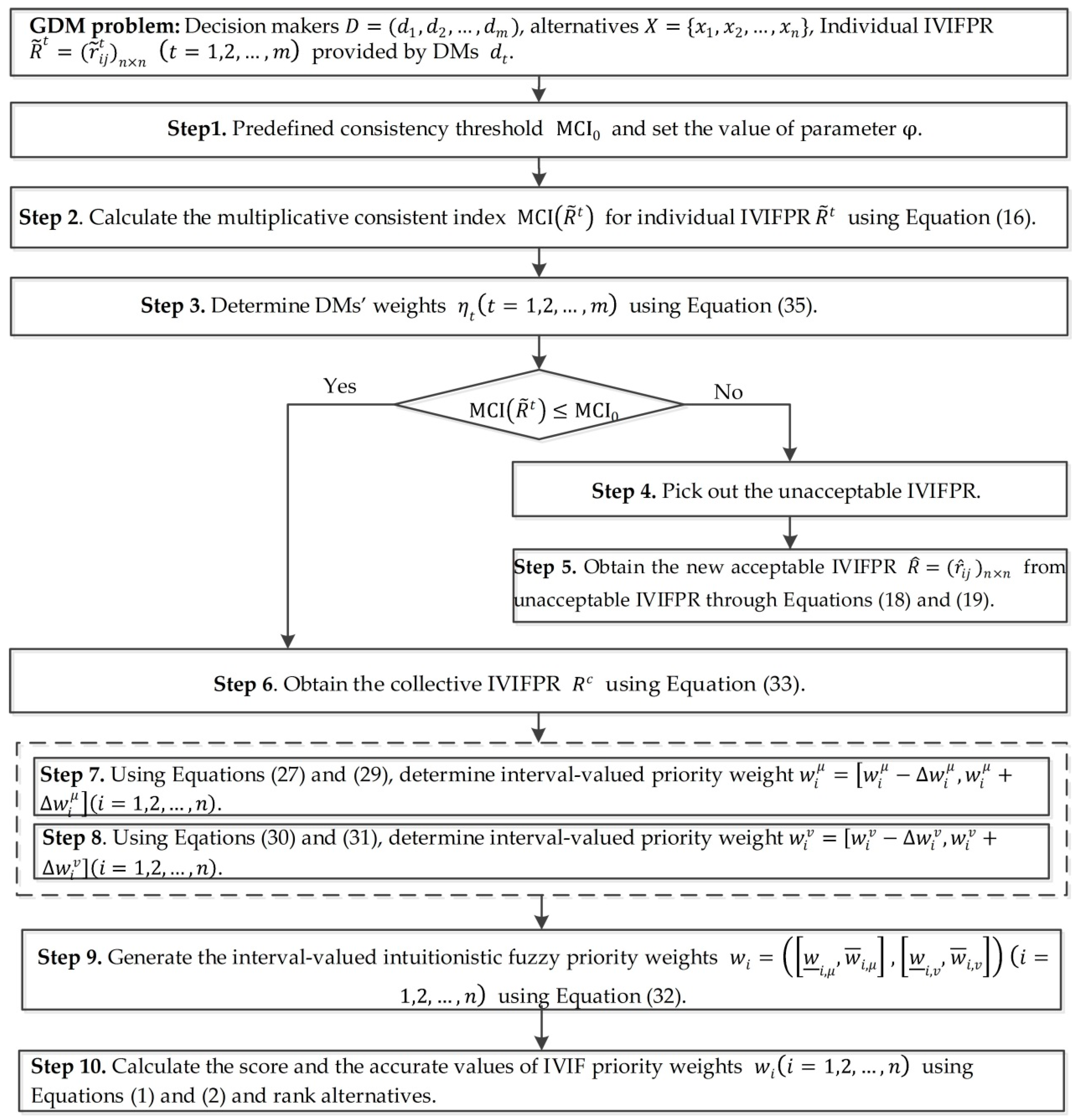
5.3. An Algorithm for GDM with IVIFPRs

Summarizing the analysis described above, a novel algorithm for GDM with IVIFPRs is proposed. The concrete steps are summarized below and in the flowchart depicted in Figure 1.

Step 1.

Predefined consistency threshold ${\mathrm{MCI}}_0$ and set the value of parameter $\mathsf{\phi }$.

Step 2.

Calculate the multiplicative consistency index $\mathrm{MCI}\left({\tilde{R}}^t\right)$ for an individual IVIFPR ${\tilde{R}}^t\left(t=1,2,\dots ,m\right)$ using Equation (16).

Step 3.

Derive DMs’ weights ${\eta }_t\left(t=1,2,\dots ,m\right)$ using Equation (35).

Step 4.

Using formula $\mathrm{MCI}\left({\tilde{R}}^t\right)\le {\mathrm{MCI}}_0$, pick out the unacceptable multiplicative consistency of IVIFPR ${\tilde{R}}^t\left(t=1,2,\dots ,m\right)$. If all IVIFPRs ${\tilde{R}}^t\left(t=1,2,\dots ,m\right)$ are acceptable multiplicative consistent, then go to Step 6; otherwise, go to Step 5.

Step 5.

Derive the acceptable multiplicative consistent IVIFPR $\widehat{R}={({\widehat{r}}_{ij})}_{n\times n}$ from unacceptable multiplicative consistent IVIFPR by Equations (18) and (19).

Step 6.

Integrate the individual IVIFPR ${\widehat{R}}^t\left(t=1,2,\dots ,m\right)$ into a collective IVIFPR ${\tilde{R}}^c$ through Equation (33).

Step 7.

Using Equations (27) and (29), determine interval-valued priority weight $w_i^{\mu }=\left[w_i^{\mu }-\Delta w_i^{\mu },w_i^{\mu }+\Delta w_i^{\mu }\right]\left(i=1,2,\dots ,n\right)$.

Step 8.

Using Equations (30) and (31), determine interval-valued priority weight $w_i^v=\left[w_i^v-\Delta w_i^v,w_i^v+\Delta w_i^v\right]\left(i=1,2,\dots ,n\right)$.

Step 9.

Generate the IVIF priority weights ${\mathrm{w}}_i=\left(\left[w_i^{\mu -},w_i^{\mu +}\right],\left[w_i^{v-},w_i^{v+}\right]\right)$ through Equation (32).

Step 10.

Using Equations (1) and (2), rank alternatives by calculating the score and the accurate values of IVIF priority weights $w_i\left(i=1,2,\dots ,n\right).$

6. A Practical Example for GDM with IVIFPRs

In this section, a practical example of enterprise innovation partner selection is provided to demonstrate the application of the proposed algorithm. The implementation of comparative analyses is to illustrate the merit of the proposed model over other methods.

6.1. A Practical Example of Enterprise Innovation Partner Selection

Owing to the limitations of resources, high risk of innovation expenditure and long commercialization cycles, an enterprise is unable to carry out innovation activities independently. In this scenario, innovation activities are generated among partners, who can share resources, technologies and critical competitiveness, by which a win-win situation among partners can be achieved. Therefore, selecting innovation partners has become a realistic choice for many firms.

There exists a company wants to select and evaluate an appropriate innovation partner. Four alternatives $\left\{x_1,x_2,x_3,x_4\right\}$ intend to bid on it. To choose the best partner, the company employs three peer review DMs/experts $\left\{d_1,d_2,d_3\right\}$ with the different professional knowledge to constitute an evaluation committee. Three DMs/experts construct one pairwise comparison judgment matrix with IVIFPRs by comparing any two partners, DMs furnish their IVIFPRs as

$${\tilde{R}}^1=\left(\begin{array}{cccc}\left(\left[0.50,0.50],[0.50,0.50\right]\right)& \left(\left[0.15,0.30],[0.65,0.70\right]\right)& \left(\left[0.30,0.35],[0.40,0.45\right]\right)& \left(\left[0.50,0.60],[0.10,0.15\right]\right)\\ \left(\left[0.65,0.70\right],\left[0.15,0.30\right]\right)& \left(\left[0.50,0.50],[0.50,0.50\right]\right)& \left(\left[0.70,0.80],[0.05,0.10\right]\right)& \left(\left[0.60,0.75],[0.10,0.20\right]\right)\\ \left(\left[0.40,0.45],[0.30,0.35\right]\right)& \left(\left[0.05,0.10],[0.70,0.80\right]\right)& \left(\left[0.50,0.50],[0.50,0.50\right]\right)& \left(\left[0.55,0.70],[0.10,0.20\right]\right)\\ \left(\left[0.10,0.15],[0.50,0.60\right]\right)& \left(\left[0.10,0.20],[0.60,0.75\right]\right)& \left(\left[0.10,0.20],[0.55,0.70\right]\right)& \left(\left[0.50,0.50],[0.50,0.50\right]\right)\end{array}\right)$$

$${\tilde{R}}^2=\left(\begin{array}{cccc}\left(\left[0.50,0.50],[0.50,0.50\right]\right)& \left(\left[0.25,0.40],[0.40,0.50\right]\right)& \left(\left[0.20,0.35],[0.60,065\right]\right)& \left(\left[0.20,0.35],[0.30,0.50\right]\right)\\ \left(\left[0.40,0.50],[0.25,0.40\right]\right)& \left(\left[0.50,0.50],[0.50,0.50\right]\right)& \left(\left[0.50,0.55],[0.30,0.40\right]\right)& \left(\left[0.55,0.70],[0.10,0.20\right]\right)\\ \left(\left[0.60,0.65],[0.20,0.35\right]\right)& \left(\left[0.30,0.40],[0.50,0.55\right]\right)& \left(\left[0.50,0.50],[0.50,0.50\right]\right)& \left(\left[0.40,0.65],[0.10,0.20\right]\right)\\ \left(\left[0.30,0.50],[0.20,0.35\right]\right)& \left(\left[0.10,0.20],[0.55,0.70\right]\right)& \left(\left[0.10,0.20],[0.40,0.65\right]\right)& \left(\left[0.50,0.50],[0.50,0.50\right]\right)\end{array}\right)$$

$${\tilde{R}}^3=\left(\begin{array}{cccc}\left(\left[0.50,0.50],[0.50,0.50\right]\right)& \left(\left[0.15,0.30],[0.40,0.50\right]\right)& \left(\left[0.10,0.30],[0.45,0.65\right]\right)& \left(\left[0.60,0.85],[0.10,0.10\right]\right)\\ \left(\left[0.40,0.50],[0.15,0.30\right]\right)& \left(\left[0.50,0.50],[0.50,0.50\right]\right)& \left(\left[0.75,0.80],[0.15,0.20\right]\right)& \left(\left[0.55,0.70],[0.10,0.15\right]\right)\\ \left(\left[0.45,0.65],[0.10,0.30\right]\right)& \left(\left[0.15,0.20],[0.75,0.80\right]\right)& \left(\left[0.50,0.50],[0.50,0.50\right]\right)& \left(\left[0.45,0.85],[0.10,0.15\right]\right)\\ \left(\left[0.10,0.10],[0.60,0.85\right]\right)& \left(\left[0.10,0.15],[0.55,0.70\right]\right)& \left(\left[0.10,0.15],[0.45,0.85\right]\right)& \left(\left[0.50,0.50],[0.50,0.50\right]\right)\end{array}\right)$$

In what follows, the proposed algorithm in this paper is employed to solve the above problem.

Step 1.

Predefine consistency threshold ${\mathrm{MCI}}_0=0.1$ and set the value of parameter $\mathsf{\phi }=0.5$.

Step 2.

Calculate the multiplicative consistency index $\mathrm{MCI}\left({\tilde{R}}^t\right)$ for individual IVIFPR ${\tilde{R}}^t\left(t=1,2,\dots ,m\right)$ using Equation (16), the results of the calculation are as follows:

$$\mathrm{MCI}\left({\tilde{R}}^1\right)=1.9679,\mathrm{MCI}\left({\tilde{R}}^2\right)=1.2745,\mathrm{MCI}\left({\tilde{R}}^3\right)= 2.1035.$$

Step 3.

Determine DMs’ weights ${\eta }_t\left(t=1,2,\dots ,m\right)$ using Equation (35).

$${\eta }_1=0.2874;{\eta }_2=0.4437;{\eta }_3=0.2689.$$

Step 4.

Using formula $\mathrm{MCI}\left({\tilde{R}}^t\right)\le {\mathrm{MCI}}_0$, all the individual IVIFPRs ${\tilde{R}}^t$ are unacceptable multiplicative consistent.

Step 5.

Solving Model (18), the optimal solutions ${\underset{\_}{\widehat{ \mu }}}_{ij}$, ${\overline{\widehat{\mu }}}_{ij}$, ${\underset{\_}{\widehat{v}}}_{ij}$ and ${\overline{\widehat{v}}}_{ij}$ for all $i,j=1,2,\dots n$ and $i<j$ are derived from unacceptable multiplicative consistent IVIFPRs ${\tilde{R}}^t\left(t=1,2,3\right)$.

Then, using Equation (19), the corresponding acceptable multiplicative consistent IVIFPRs ${\widehat{R}}^t={({\widehat{r}}_{ij})}_{n\times n}\left(t=1,2,3\right)$ are generated as

$${\widehat{R}}^1=\left(\begin{array}{cccc}\left(\left[0.50,0.50],[0.50,0.50\right]\right)& \left(\left[0.16,0.24],[0.66,0.70\right]\right)& \left(\left[0.30,0.39],[0.40,0.45\right]\right)& \left(\left[0.37,0.60],[0.10,0.15\right]\right)\\ \left(\left[0.66,0.70\right],\left[0.16,0.24\right]\right)& \left(\left[0.50,0.50],[0.50,0.50\right]\right)& \left(\left[0.70,0.70],[0.23,0.23\right]\right)& \left(\left[0.74,0.83],[0.06,0.07\right]\right)\\ \left(\left[0.40,0.45],[0.30,0.39\right]\right)& \left(\left[0.23,0.23],[0.70,0.70\right]\right)& \left(\left[0.50,0.50],[0.50,0.50\right]\right)& \left(\left[0.55,0.70],[0.14,0.20\right]\right)\\ \left(\left[0.10,0.15],[0.37,0.60\right]\right)& \left(\left[0.06,0.07],[0.74,0.83\right]\right)& \left(\left[0.14,0.20],[0.55,0.70\right]\right)& \left(\left[0.50,0.50],[0.50,0.50\right]\right)\end{array}\right)$$

$${\widehat{R}}^2=\left(\begin{array}{cccc}\left(\left[0.50,0.50\right],\left[0.50,0.50\right]\right)& \left(\left[0.25,0.30\right],\left[0.70,0.70\right]\right)& \left(\left[0.23,0.35\right],\left[0.60,0.65\right]\right)& \left(\left[0.20,0.47\right],\left[0.22,0.39\right]\right)\\ \left(\left[0.70,0.70\right],\left[0.25,0.30\right]\right)& \left(\left[0.50,0.50\right],\left[0.50,0.50\right]\right)& \left(\left[0.50,0.55\right],\left[0.37,0.42\right]\right)& \left(\left[0.45,0.70\right],\left[0.10,0.20\right]\right)\\ \left(\left[0.60,0.65\right],\left[0.23,0.35\right]\right)& \left(\left[0.37,0.42\right],\left[0.50,0.55\right]\right)& \left(\left[0.50,0.50\right],\left[0.50,0.50\right]\right)& \left(\left[0.43,0.65\right],\left[0.15,0.24\right]\right)\\ \left(\left[0.22,0.39\right],\left[0.20,0.47\right]\right)& \left(\left[0.10,0.20\right],\left[0.45,0.70\right]\right)& \left(\left[0.15,0.24\right],\left[0.43,0.65\right]\right)& \left(\left[0.50,0.50\right],\left[0.50,0.50\right]\right)\end{array}\right)$$

$${\widehat{R}}^3=\left(\begin{array}{cccc}\left(\left[0.50,0.50\right],\left[0.50,0.50\right]\right)& \left(\left[0.15,0.30\right],\left[0.50,0.50\right]\right)& \left(\left[0.21,0.39\right],\left[0.40,0.40\right]\right)& \left(\left[0.19,0.80\right],\left[0.10,0.10\right]\right)\\ \left(\left[0.50,0.50\right],\left[0.15,0.30\right]\right)& \left(\left[0.50,0.50\right],\left[0.50,0.50\right]\right)& \left(\left[0.63,0.63\right],\left[0.37,0.37\right]\right)& \left(\left[0.50,0.89\right],\left[0.10,0.11\right]\right)\\ \left(\left[0.40,0.40\right],\left[0.21,0.39\right]\right)& \left(\left[0.37,0.37\right],\left[0.63,0.63\right]\right)& \left(\left[0.50,0.50\right],\left[0.50,0.50\right]\right)& \left(\left[0.45,0.85\right],\left[0.14,0.15\right]\right)\\ \left(\left[0.10,0.10\right],\left[0.19,0.80\right]\right)& \left(\left[0.10,0.11\right],\left[0.50,0.89\right]\right)& \left(\left[0.14,0.15\right],\left[0.45,0.85\right]\right)& \left(\left[0.50,0.50\right],\left[0.50,0.50\right]\right)\end{array}\right)$$

Step 6.

Integrating the acceptable multiplicative consistent IVIFPR $\widehat{R}={({\widehat{r}}_{ij})}_{n\times n}$ by DMs’ weights ${\eta }_t\left(t=1,2,3\right)$, the collective IVIFPR $R^c$ is generated using Equation (33) as follows:

$$R^c=\left(\begin{array}{cccc}\left(\left[0.50,0.50\right],\left[0.50,0.50\right]\right)& \left(\left[0.20,0.28\right],\left[0.63,0.65\right]\right)& \left(\left[0.24,0.37\right],\left[0.49,0.53\right]\right)& \left(\left[0.25,0.60\right],\left[0.15,0.24\right]\right)\\ \left(\left[0.63,0.65\right],\left[0.20,0.28\right]\right)& \left(\left[0.50,0.50\right],\left[0.50,0.50\right]\right)& \left(\left[0.59,0.61\right],\left[0.33,0.35\right]\right)& \left(\left[0.56,0.79\right],\left[0.09,0.14\right]\right)\\ \left(\left[0.49,0.53\right],\left[0.24,0.37\right]\right)& \left(\left[0.33,0.35\right],\left[0.59,0.61\right]\right)& \left(\left[0.50,0.50\right],\left[0.50,0.50\right]\right)& \left(\left[0.47,0.72\right],\left[0.14,0.20\right]\right)\\ \left(\left[0.15,0.24\right],\left[0.25,0.60\right]\right)& \left(\left[0.09,0.14\right],\left[0.56,0.79\right]\right)& \left(\left[0.14,0.20\right],\left[0.47,0.72\right]\right)& \left(\left[0.50,0.50\right],\left[0.50,0.50\right]\right)\end{array}\right)$$

Step 7.

Using Equations (27) and (29), IVIFPR priority weight vector $w_i^{\mu }=\left[w_i^{\mu }-\Delta w_i^{\mu },w_i^{\mu }+\Delta w_i^{\mu }\right]\left(i=1,2,3,4\right)$ are generated as follows:

$$w_1^{\mu }=\left[0.1900,0.2219\right],w_2^{\mu }=\left[0.2847,0.3050\right],$$

$$w_3^{\mu }=\left[0.2535,0.2769\right], w_4^{\mu }=\left[0.2137,0.2542\right].$$

Step 8.

Using Equations (30) and (31), IVIFPR priority weight vector $w_i^v=\left[w_i^v-\Delta w_i^v,w_i^v+\Delta w_i^v\right]\left(i=1,2,3,4\right)$ are generated as follows:

$$w_1^v=\left[0.2587,0.2668\right],w_2^v=\left[0.3047,0.3095\right],$$

$$w_3^v=\left[0.2616,0.2676\right], w_4^v=\left[0.1606,0.1705\right].$$

Step 9.

By Equation (32), the IVIFPR priority weights ${\mathrm{w}}_i=\left(\left[w_i^{\mu -},w_i^{\mu +}\right],\left[w_i^{v-},w_i^{v+}\right]\right)\left(i=1,2,3,4\right)$ are derived as follows:

$${\mathrm{w}}_1=\left(\left[0.1821,0.2479\right],\left[0.7028,0.7459\right]\right),{\mathrm{w}}_2=\left(\left[0.2729,0.2921\right],\left[0.6619,0.6662\right]\right),$$

$${\mathrm{w}}_3=\left(\left[0.2430,0.2507\right],\left[0.6931,0.7020\right]\right),{\mathrm{w}}_4=\left(\left[0.1539,0.2049\right],\left[0.7149,0.7951\right]\right).$$

Step 10.

According to Definition 3, the scores function of IVIFV belongs to the interval [−1, 1], and its associating weight should be a non-negative number. Therefore, the score function defined in Definition 3 should be modified to facilitate this situation under the conditions of without changing any of the following basic properties

$$\mathrm{S}\left(\tilde{\delta }\right)=\frac{\underset{\_}{\mu }-\underset{\_}{v}+\overline{\mu }-\overline{v}+2}{4}$$

(36)

Through Equation (36), the scores function $S\left(w_i\right)$ and accuracy degrees of $H\left(w_i\right)$ of $w_i\left(i=1,2,3,4\right)$ are obtained as $S\left(w_1\right)=0.2454$, $S\left(w_2\right)=0.3092$, $S\left(w_3\right)=0.2747$, $S\left(w_4\right)=0.2122$, $H\left(w_1\right)=0.9394$, $H\left(w_2\right)=0.9466$, $H\left(w_3\right)=0.9444$, $H\left(w_4\right)=0.9344$,

Thus, descending scores function $S\left(w_i\right)\left(i=1,2,3,4\right)$ and accuracy degrees $H\left(w_i\right)\left(i=1,2,3,4\right)$, the ranking order of alternatives is $x_2>x_3>x_1>x_4$, and $x_2$ is the best partner.

Additionally, when $\mathsf{\phi }$ takes different values, we get the associated calculation results and ranking orders shown

Table 1. Computation results and ranking orders for different values of parameters $\mathsf{\phi }$ with ${\mathrm{MCI}}_0=0.1$

$\mathit{\phi }$	$\mathit{S}\left({\mathit{w}}_1\right)$	$\mathit{H}\left({\mathit{w}}_1\right)$	$\mathit{S}\left({\mathit{w}}_2\right)$	$\mathit{H}\left({\mathit{w}}_2\right)$	$\mathit{S}\left({\mathit{w}}_3\right)$	$\mathit{H}\left({\mathit{w}}_3\right)$	$\mathit{S}\left({\mathit{w}}_4\right)$	$\mathit{H}\left({\mathit{w}}_4\right)$	Ranking Order
0	0.2449	0.9393	0.3092	0.9461	0.2752	0.9442	0.2122	0.9338	$x_2>x_3>x_1>x_4$
0.1	0.2451	0.9393	0.3091	0.9461	0.2751	0.9443	0.2122	0.9339	$x_2>x_3>x_1>x_4$
0.2	0.2451	0.9395	0.3090	0.9463	0.2750	0.9445	0.2123	0.9341	$x_2>x_3>x_1>x_4$
0.3	0.2451	0.9395	0.3091	0.9464	0.2749	0.9445	0.2123	0.9341	$x_2>x_3>x_1>x_4$
0.4	0.2450	0.9396	0.3093	0.9466	0.2749	0.9446	0.2121	0.9343	$x_2>x_3>x_1>x_4$
0.5	0.2454	0.9394	0.3092	0.9466	0.2747	0.9444	0.2122	0.9344	$x_2>x_3>x_1>x_4$
0.6	0.2454	0.9394	0.3094	0.9466	0.2745	0.9445	0.2121	0.9345	$x_2>x_3>x_1>x_4$
0.7	0.2453	0.9389	0.3090	0.9461	0.2754	0.9440	0.2124	0.9342	$x_2>x_3>x_1>x_4$
0.8	0.2452	0.9389	0.3089	0.9461	0.2755	0.9441	0.2125	0.9341	$x_2>x_3>x_1>x_4$
0.9	0.2472	0.9370	0.3116	0.9456	0.2715	0.9421	0.2108	0.9348	$x_2>x_3>x_1>x_4$
1	0.2460	0.9370	0.3101	0.9463	0.2722	0.9418	0.2110	0.9371	$x_2>x_3>x_1>x_4$

. For different consistency threshold ${\mathrm{MCI}}_0$, the corresponding computation results are listed in

Table 2. Computation results and ranking orders for different values of parameters ${\mathrm{MCI}}_0$ with $\mathsf{\phi }=\mathrm{0.5.}$

Parameter	$\mathit{S}\left({\mathit{w}}_1\right)$	$\mathit{H}\left({\mathit{w}}_1\right)$	$\mathit{S}\left({\mathit{w}}_2\right)$	$\mathit{H}\left({\mathit{w}}_2\right)$	$\mathit{S}\left({\mathit{w}}_3\right)$	$\mathit{H}\left({\mathit{w}}_3\right)$	$\mathit{S}\left({\mathit{w}}_4\right)$	$\mathit{H}\left({\mathit{w}}_4\right)$	Ranking Order
${\mathrm{MCI}}_0=0.1$	0.2454	0.9394	0.3092	0.9466	0.2747	0.9444	0.2122	0.9344	$x_2>x_3>x_1>x_4$
${\mathrm{MCI}}_0=0$	0.2489	0.9348	0.3092	0.9423	0.2732	0.9400	0.2112	0.9310	$x_2>x_3>x_1>x_4$
${\mathrm{MCI}}_0=0.01$	0.2487	0.9350	0.3095	0.9426	0.2730	0.9401	0.2112	0.9312	$x_2>x_3>x_1>x_4$

.

It can see from Table 1 and Table 2 that the ranking order results are always $x_2>x_3>x_1>x_4$ and the best partner is $x_2$. Moreover, the ranking order result derived from the absolutely multiplicative consistent IVIFPR (i.e., ${\mathrm{MCI}}_0=0$ and $\mathsf{\phi }=0.5$) is the same as other situations in Table 2. Consequently, it may be robust and applicable to directly adopt the proposed algorithm in this paper for addressing practical GDM with IVIFPR.

6.2. Comparative Analyses

In order to reveal the superiority of our proposed method, this subsection concentrates on comparative analyses with Wan’s method [12] and other existing GDM methods [6,18].

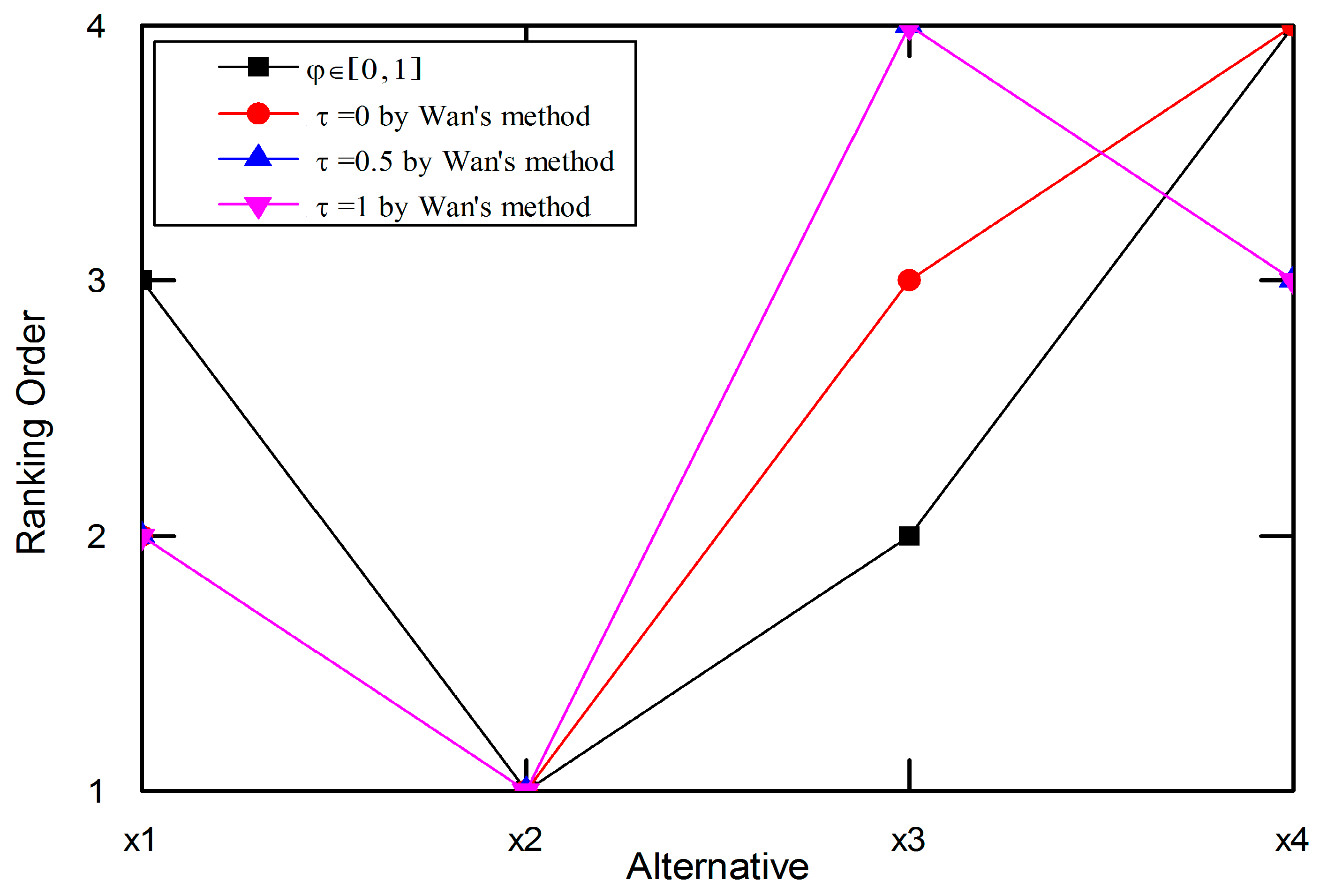
6.2.1. Comparison with Wan’s Method

We adopt Wan’s method [12] to solve the practical example in 6.1. Similar to Wan’s method, set the consistent threshold value $MC{I}_0=0.1$ and group’s opinions $l=0.5$, different DMs’ weight vectors ${\eta }_i\left(i=1,2,3\right)$ can be obtained when taking different values of parameter $\mathsf{\tau }$, which denotes three particular principles of minority, majority and compromise principle if $\mathsf{\tau }=0,$ $1$ and $0.5$, respectively. The calculation results are shown in

Table 3. Computation results for different DMs’ weights ${\eta }_i\left(i=1,2,3\right)$ by Wan’s method [12].

$\mathsf{\tau }.$	$\mathsf{\tau }=0$	$\mathsf{\tau }=0.5$	$\mathsf{\tau }=1$
$\eta$	$\eta ={\left(0.3888,0.3056,0.3056\right)}^T$	$\eta ={\left(0.4078,0.2718,0.3204\right)}^T$	$\eta ={\left(0.400,0.2000,0.4000\right)}^T$
$w_1$	$\left(\left[0.1165,0.2287\right],\left[0.6715,0.6715\right]\right)$	$\left(\left[0.1151,0.2309\right],\left[0.6729,0.6729\right]\right)$	$\left(\left[0.1109,0.2435\right],\left[0.6698,0.6698\right]\right)$
$w_2$	$\left(\left[0.3208,0.4248\right],\left[0.4754,0.5116\right]\right)$	$\left(\left[0.3262,0.4324\right],\left[0.4689,0.5034\right]\right)$	$\left(\left[0.3262,0.4413\right],\left[0.4624,0.4931\right]\right)$
$w_3$	$\left(\left[0.0831,0.1304\right],\left[0.6967,0.8696\right]\right)$	$\left(\left[0.0797,0.1262\right],\left[0.8738,0.8738\right]\right)$	$\left(\left[0.0739,0.1185\right],\left[0.8815,0.8815\right]\right)$
$w_4$	$\left(\left[0.0165,0.0527\right],\left[0.7115,0.8475\right]\right)$	$\left(\left[0.0156,0.0501\right],\left[0.7725,0.8537\right]\right)$	$\left(\left[0.0137,0.0444\right],\left[0.7671,0.8689\right]\right)$
$T\left(w_1\right)$	0.4915	0.4898	0.4957
$T\left(w_2\right)$	0.6783	0.6836	0.6910
$T\left(w_3\right)$	0.3711	0.3644	0.3543
$T\left(w_4\right)$	0.3702	0.3665	0.3655
R.O.	$x_2>x_1>x_3>x_4$	$x_2>x_1>x_4>x_3$	$x_2>x_1>x_4>x_3$

Note: 1. when $l=0.5$, $T\left(w_i\right)\left(i=1,2,34\right)$ denotes the comprehensive closeness degree defined in Wan’s method [12]. 2. “R.O.” is an abbreviation for “ranking order”.

. Additionally, when ${\mathrm{MCI}}_0=0.1$, the ranking orders of alternatives for different values of parameters ($\phi$ in the proposed algorithm and $\mathsf{\tau }$ in Wan’s method [12]) are depicted in Figure 2.

Table 3 and Figure 2 reveal that the ranking order results are different, but the best alternative is $x_2$, which is the same as the proposed algorithm. Compared with Wan’s method [12], the proposed algorithm has the following advantages.

(1)

When measuring the consistency degree of an IVIFPR, the proposed algorithm is more straightforward than Wan’s method [12]. Wan’s method [12] needs resort to two particular IFPR matrices from original IVIFPR. In contrast, the proposed algorithm directly performs the measurement work only depending on original IVIFPR, which can avoid losing original information via Wan’s method [12].

(2)

In terms of repairing and improving the unacceptable multiplicative consistent IVIFPR, different from the iterative algorithms proposed in Wan’s method [12], this paper directly built an optimization model through considering various decision-making principles, which can quickly obtain the acceptable consistent IVIFPR and flexibly reflect the principles of decision making.

(3)

For determining priority weights of alternatives, Wan’s method [12] constructed a goal optimization model which needs numerous computations. On the contrary, the proposed algorithm determines IVIF priority weights by extending error-analysis-based priority method to IVIFPR environment, which is a time-saving and simple calculation.

6.2.2. Comparison with Other Existing Methods

Except for the above quantitatively comparative analysis, this subsection implements a qualitatively comparative analysis by using the existing GDM methods [6,18].

(1)

The concerns of these methods are different. Method [6] studied the consistent and consensus in GDM with IFPR, whereas Method [18] and the proposed algorithm concentrate on the multiplicative consistency of IVIFPR. The discrepancy is that Method [18] focused on the multiplicative transitivity of IVIFPR and improving the consistency of an inconsistent IVIFPR, while the proposed algorithm is devoted to judging and measuring the multiplicative consistency degree of an IVIFPR and address the GDM with IVIFPRs.

(2)

Method [18] investigated an acceptable property of multiplicative consistency of IVIFPR and introduced some associated concepts of IVIFPR (i.e., the approximate, the perfect and the acceptable multiplicative consistent IVIFPR), but the multiplicative consistency degree of an IVIFPR cannot be obtained in Method [18]. Following the work of Method [18], based on two principles of decision making (the majority and minority principles), this paper proposes a new definition of consistency index of an IVIFPR, which can measure the multiplicative consistency degree of an IVIFPR.

(3)

Regarding to priority weight determination, Methods [6,18] cannot provide any tools or methods determine priority weights. However, this paper extends error-analysis-based approach in IVIFPR to determine priority weights, and it is worth noting that the proposed algorithm can reduce the complexity of the calculation.

7. Conclusions

With the high complexity and uncertainty in (group) decision-making environments, IVIFPRs have attracted increasing attention. In this paper, we focus on the acceptability measurement and determination of IVIF priority weights based on IVIFPRs. The main contributions are outlined as follows.

(1)

A new definition of consistency index is defined to measure whether an IVIFPR is of acceptable multiplicative consistency. A common feature is that it can complete the measurement work only employing individual IVIFPRs themselves.

(2)

An optimization model is constructed to improve the consistency degree for those IVIFPRs that not attain the acceptable level. Moreover, the obtained IVIFPRs can retain the preference information given by the initial IVIFPRs, for the most part.

(3)

An error-analysis-based extension method is proposed to determine IVIF priority weights from the acceptable IVIFPR. It can help the decision maker to obtain the reasonable and identified decision-making results.

(4)

A step-by-step algorithm is developed for solving GDM with IVIFPRs, and a practical example is presented to demonstrate its effectiveness and practicality. The results in this paper are very important for the application of IVIFPR in GDM.

However, the proposed algorithm has some drawbacks, i.e., current research framework assumes that the parameter values of the consistency threshold ${\mathrm{MCI}}_0$ and the DMs’ risk attitude $\mathsf{\phi }$ are predetermined. Sometime these requirements are too difficult for decision makers. Moreover, we do not present the proposed algorithm for solving GDM with incomplete IVIFPRs. Therefore, for future research, under the current framework, we will focus on investigating the parameter values of the consistency thresholds ${\mathrm{MCI}}_0$ and DMs’ risk attitude $\mathsf{\phi }$ of IVIFPR as well as a consensus approach for GDM with incomplete IVIFPRs.

References

1. Orlovsky, S.A. Decision-making with a fuzzy preference relation. Fuzzy Sets Syst. 1978, 1, 155–167. [Google Scholar] [CrossRef]
2. Yan, H.B.; Ma, T. A group decision-making approach to uncertain quality function deployment based on fuzzy preference relation and fuzzy majority. Eur. J. Oper. Res. 2015, 241, 815–829. [Google Scholar] [CrossRef]
3. Saaty, T.L. The Analytic Hierarchy Process: Planning, Priority Setting, Resource Allocation; McGraw-Hill: New York, NY, USA, 1980. [Google Scholar]
4. Wang, Y.M.; Fan, Z.P.; Hua, Z.S. A chi-square method for obtaining a priority vector from multiplicative and fuzzy preference relations. Eur. J. Oper. Res. 2007, 182, 356–366. [Google Scholar] [CrossRef]
5. Chu, J.; Liu, X.; Wang, Y.; Chin, K.S. A group decision making model considering both the additive consistency and group consensus of intuitionistic fuzzy preference relations. Comput. Ind. Eng. 2016, 101, 227–242. [Google Scholar] [CrossRef]
6. Xu, G.L.; Wan, S.P.; Wang, F.; Dong, J.Y.; Zeng, Y.F. Mathematical programming methods for consistency and consensus in group decision making with intuitionistic fuzzy preference relations. Knowl.-Based Syst. 2016, 98, 30–43. [Google Scholar] [CrossRef]
7. Wan, S.; Wang, F.; Dong, J. A group decision making method with interval valued fuzzy preference relation based on the geometric consistency. Inf. Fusion 2017, 40, 87–100. [Google Scholar] [CrossRef]
8. Meng, F.Y.; An, Q.X.; Tan, C.Q.; Chen, X.H. An Approach for Group Decision Making With Interval Fuzzy Preference Relations Based on Additive Consistency and Consensus Analysis. IEEE Trans. Syst. Man Cybern. Syst. 2016, PP, 1–14. [Google Scholar] [CrossRef]
9. Wan, S.P.; Wang, F.; Dong, J.Y. Additive consistent interval-valued Atanassov intuitionistic fuzzy preference relation and likelihood comparison algorithm based group decision making. Eur. J. Oper. Res. 2017, 263, 571–582. [Google Scholar] [CrossRef]
10. Wan, S.P.; Wang, F.; Dong, J.Y. A Three-Phase Method for Group Decision Making With Interval-Valued Intuitionistic Fuzzy Preference Relations. IEEE Trans. Fuzzy Syst. 2018, 26, 998–1010. [Google Scholar] [CrossRef]
11. Chu, J.; Liu, X.; Wang, L.; Wang, Y. A Group Decision Making Approach Based on Newly Defined Additively Consistent Interval-Valued Intuitionistic Preference Relations. Int. J. Fuzzy Syst. 2017, 20, 1027–1046. [Google Scholar] [CrossRef]
12. Wan, S.P.; Xu, G.L.; Dong, J.Y. A novel method for group decision making with interval-valued Atanassov intuitionistic fuzzy preference relations. Inf. Sci. 2016, 372, 53–71. [Google Scholar] [CrossRef]
13. Liu, F.; Aiwu, G.; Lukovac, V.; Vukic, M. A multicriteria model for the selection of the transport service provider: A single valued neutrosophic DEMATEL multicriteria model. Decis. Mak. Appl. Manag. Eng 2018, 1, 121–130. [Google Scholar] [CrossRef]
14. Petrović, I.; Kankaraš, M. DEMATEL-AHP multi-criteria decision making model for the selection and evaluation of criteria for selecting an aircraft for the protection of air traffic. Decis. Mak. Appl. Manag. Eng 2018, 1, 93–110. [Google Scholar] [CrossRef]
15. Ze-Shui, X.U.; Chen, J. Approach to Group Decision Making Based on Interval-Valued Intuitionistic Judgment Matrices. Syst. Eng.-Theory Pract. 2007, 27, 126–133. [Google Scholar]
16. Xu, Z.S.; Cai, X.Q. Incomplete interval-valued intuitionistic fuzzy preference relations. Int. J. Gener. Syst. 2009, 38, 871–886. [Google Scholar] [CrossRef]
17. Xu, Z.; Cai, X. Group Decision Making with Incomplete Interval-Valued Intuitionistic Preference Relations. Group Decis. Negotiat. 2015, 24, 193–215. [Google Scholar] [CrossRef]
18. Liao, H.C.; Xu, Z.S.; Xia, M.M. Multiplicative consistency of interval-valued intuitionistic fuzzy preference relation. J. Intell. Fuzzy Syst. 2014, 27, 2969–2985. [Google Scholar]
19. Meng, F.Y.; Tang, J.; Wang, P.; Chen, X.H. A programming-based algorithm for interval-valued intuitionistic fuzzy group decision making. Knowl.-Based Syst. 2018, 144, 122–143. [Google Scholar] [CrossRef]
20. Mukhametzyanov, I.; Pamucar, D. A sensitivity analysis in MCDM problems: A statistical approach. Decis. Mak. Appl. Manag. Eng. 2018, 1, 1–20. [Google Scholar] [CrossRef]
21. Wang, Z.J.; Lin, J. Acceptability measurement and priority weight elicitation of triangular fuzzy multiplicative preference relations based on geometric consistency and uncertainty indices. Inf. Sci. 2017, 402, 105–123. [Google Scholar] [CrossRef]
22. Xu, Z.; Yager, R.R. Intuitionistic and interval-valued intutionistic fuzzy preference relations and their measures of similarity for the evaluation of agreement within a group. Fuzzy Optim. Decis. Mak. 2009, 8, 123–139. [Google Scholar] [CrossRef]
23. Wu, J.; Chiclana, F. Non-dominance and attitudinal prioritisation methods for intuitionistic and interval-valued intuitionistic fuzzy preference relations. Expert Syst. Appl. 2012, 39, 13409–13416. [Google Scholar] [CrossRef]
24. Yue, C. A geometric approach for ranking interval-valued intuitionistic fuzzy numbers with an application to group decision-making. Comput. Ind. Eng. 2016, 102, 233–245. [Google Scholar] [CrossRef]
25. Zhou, H.; Ma, X.Y.; Zhou, L.G.; Chen, H.Y.; Ding, W.R. A Novel Approach to Group Decision-Making with Interval-Valued Intuitionistic Fuzzy Preference Relations via Shapley Value. Int. J. Fuzzy Syst. 2018, 20, 1172–1187. [Google Scholar] [CrossRef]
26. Xu, Z.S. An error-analysis-based method for the priority of an intuitionistic preference relation in decision making. Knowl.-Based Syst. 2012, 33, 173–179. [Google Scholar] [CrossRef]
27. Xu, Z. On Compatibility of Interval Fuzzy Preference Relations. Fuzzy Optim. Decis. Mak. 2004, 3, 217–225. [Google Scholar] [CrossRef]
28. Atanassov, K.; Gargov, G. Interval Valued Intuitionistic Fuzzy-Sets. Fuzzy Set Syst. 1989, 31, 343–349. [Google Scholar] [CrossRef]
29. Yager, R.R. Induced aggregation operators. Fuzzy Set Syst. 2003, 137, 59–69. [Google Scholar] [CrossRef]
30. Pugh, E.M.; Winslow, G.H. The Analysis of Physical Measurements; Addison-Wesley: Reading, MA, USA, 1966. [Google Scholar]
31. Xu, Y.; Herrera, F.; Wang, H. A distance-based framework to deal with ordinal and additive inconsistencies for fuzzy reciprocal preference relations. Inf. Sci. 2016, 328, 189–205. [Google Scholar] [CrossRef]
32. Bustince, H. Conjuntos Intuicionistas e Intervalo Valorados Difusos: Propiedades y Construccion, Relaciones Intuicionistas Fuzzy. Ph.D. Thesis, Universidad Publica de Navarra, Pamplona, Spain, 1994. [Google Scholar]
33. Shui, X.Z. Algorithm for priority of fuzzy complementary judgement matrix. J. Syst. Eng. 2001, 16, 311–314. [Google Scholar]
Figure 1. The flowchart of the whole steps for group decision making (GDM) with interval-valued intuitionistic fuzzy preference relations (IVIFPRs).
Algorithms 11 00182 g001
Figure 2. Ranking orders of alternative by different methods with MCI 0 = 0.1.
Algorithms 11 00182 g002