Article

Measuring the Impact of Financial News and Social Media on Stock Market Modeling Using Time Series Mining Techniques

by
Foteini Kollintza-Kyriakoulia
1,
Manolis Maragoudakis
1,* and
Anastasia Krithara
2
1
Department of Information and Communication Systems Engineering, University of the Aegean, GR-83200 Samos, Greece
2
Institute of Informatics and Telecommunications, National Center for Scientific Center “Demokritos”, GR-15310 Athens, Greece
*
Author to whom correspondence should be addressed.
Algorithms 2018, 11(11), 181; https://doi.org/10.3390/a11110181
Submission received: 23 August 2018 / Revised: 17 October 2018 / Accepted: 23 October 2018 / Published: 6 November 2018
(This article belongs to the Special Issue Humanistic Data Mining: Tools and Applications)

Abstract

:
In this work, we study the task of predicting the closing price of the following day of a stock, based on technical analysis, news articles and public opinions. The intuition of this study lies in the fact that technical analysis contains information about the event, but not the cause of the change, while data like news articles and public opinions may be interpreted as a cause. The paper uses time series analysis techniques such as Symbolic Aggregate Approximation (SAX) and Dynamic Time Warping (DTW) to study the existence of a relation between price data and textual information, either from news or social media. Pattern matching techniques from time series data are also incorporated, in order to experimentally validate potential correlations of price and textual information within given time periods. The ultimate goal is to create a forecasting model that exploits the previously discovered patterns in order to augment the forecasting accuracy. Results obtained from the experimental phase are promising. The performance of the classifier shows clear signs of improvement and robustness within the time periods where patterns between stock price and the textual information have been identified, compared to the periods where patterns did not exist.

1. Introduction

One of the most challenging tasks faced by researchers in modeling dynamic systems is the creation of accurate stock market forecast models. Dynamic systems are governed by complexity. Volatility is another characteristic of market dynamics. As a result, much controversy has been caused as to whether such a forecasting method could exist. Therefore, two main strategies have been encapsulated by analysts, namely the fundamental and the technical strategy [1]. The former states that the stock market change of prices derives from a security’s relative data. In a fundamentalist trading philosophy, the price of a security can be determined through the nuts and bolts of financial numbers. These numbers are derived from the overall economy, the particular industry’s sector or, most typically, from the company dynamics. Parameters such as inflation, joblessness, return on equity (ROE), debt levels and individual price to earnings (PE) ratios have been identified as components that aid towards determining the price of a stock.
On the other axis, that of technical analysis, research is based on the belief that market timing is the key concept. Technicians utilize historical data in the form of charts and figures in order to identify trends in price. These strategists assume that market timing is critical, and thus, opportunities can arise through the careful investigation of historical price and volume trends, comparing them against current prices. Technical analysts also support the claim that certain high/low psychological price barriers exist, such as support and resistance levels where opportunities may lurk. Furthermore, an additional assumption that is adopted is that price movements are not completely unsystematic. Nevertheless, according to a variety of researchers, the goal is not to question the predictability of financial time series data, but to discover a good model, able to cope with the dynamics of stock market.
Even though many researchers adopt the aforementioned categorization between fundamentalist trading philosophy and technical analysis, we are of the opinion that good fundamental knowledge could be combined with patterns derived from technical analysis in an attempt to overcome issues such as asymmetric or erroneous information.
Towards the latter path, stock market analysis utilizing sophisticated Information and Communication Technology (ICT) has gained a significant amount of attention. Over the past few years, there has been an increasing focus on the development of modeling systems, especially when the expected outcomes appear to yield significant profits to the investors’ portfolios. In alignment with modern globalized economy and the expansion of social media platforms that allow for rapid exchange of information among users, the available resources are gradually becoming more plentiful, thus difficult to be analyzed by typical statistical tools. Consequently, financial experts emphasize the utilization of data mining methods, mainly due to the quantity and the increased rate by which data are being formed. Thus far, there has been a significant number of research papers that have focused on applying data mining methods solely upon past data from stock bond prices and other technical indicators. Nevertheless, throughout recent studies, prediction is also based on textual information, based on the logical assumption that the course of a stock price can be influenced by news articles, ranging from companies’ releases and local politics to news of superpower economies [2].
However, gaining unrestricted electronic access to news data was not feasible earlier than 2000. Nowadays, news is easily accessible, insights on important information such as inside company data are fairly inexpensive and domain expert estimations emerge from a vast pool of economists, statisticians, journalists, etc., through the Internet. Despite the great amount of data, advances in natural language processing and data mining allow for effective computerized representation of unstructured document collections, analysis for pattern extraction and discovery of relationships between documents and time-stamped data streams of stock market quotes. Not only news can play an important role towards influencing stock market trends. Public attitude states or sentiment, as expressed through various means that promote inter-connectivity, such as Web 2.0 platforms, may also play a similarly important role. Targeted research in the domain of psychology has proven that emotions in addition to information have a direct impact on human decision-making [3]. Therefore, a logical assumption would be for someone to consider opinions originating from social media as an additional factor that could also affect stock market values.
In this work, the main objective is to study and model the impact of technical analysis, news articles and public opinions for the task of predicting the closing price of the stocks. The importance of this study lies in the fact that technical analysis contains the event and not the cause of the change, while textual data may be interpreted as a cause. Despite the fact that there are several attempts that have incorporated technical analysis data with textual information, we are motivated by the fact that all of these works take a sliding window of time into consideration, i.e., they only focus on the characteristics that are very close to the event being examined in each time period. Therefore, we propose a totally different approach, which is based on the potential periodicity of events, that could further improve forecasting performance. The paper uses time series analysis techniques such as Symbolic Aggregate Approximation (SAX) and Dynamic Time Warping (DTW) to study the existence of a relation between price data and textual information, either from news or social media. In order to accomplish this first goal, pattern matching techniques from time series data are incorporated. Upon identification of such patterns and their periodicity, the second goal is the main objective described above, namely creating a forecasting model that exploits the previously discovered patterns in order to augment the forecasting accuracy. Results obtained from the experimental phase are promising. The performance of the classifier shows clear signs of improvement and robustness within the time periods where patterns between stock price and the textual information have been identified, compared to the periods where patterns did not exist. Certainly, as it is tedious for a human investor to read all daily news and public reactions concerning a company and other financial information, a prediction system that could analyze such textual resources and find relationships with price movement at future time windows is beneficial.
The paper is structured as follows: Section 2 provides an overview of the literature concerning stock market prediction from textual and financial resources using data mining techniques. Section 3 gives some theoretical background, while in Section 4, the methodology of the approach is presented. Section 5 presents the experimental setting and the obtained results. In Section 6, the shortcomings of the paper are presented, and Section 7 concludes the paper.

2. Previous Work

The stock market is an area of great scientific interest because of the large volume of information that accumulates daily. Financial news articles and social media such as Twitter are believed to have an impact on stock price return. Data mining can yield a very large profit, and that is one reason why many companies have invested in information technology. To this end, there are several previous works in this area. In the paper [4], the relevant news by type and tone was identified, in order to provide more evidence of the relationship between stock price changes and information. Initially, [5] showed that there is actually little relationship between stock prices and news. The financial literature has been unable to reverse this finding. However, [4], using the advantages of text analysis, demonstrated a correlation between the stock price and news. They found that when the information can be identified and the tone (positive or negative) of this information can be determined, there is a closer relationship between the stock and information.
The paper [6] examined the correlation of a micro-blogging platform, Twitter, with events of the stock market, such as changes in price and the value/volume of transactions. In particular, they collected messages related to a number of companies and looked for correlations between the stock market events and features extracted from the messages. They have categorized the features into two groups: in the first group, the overall activity on Twitter was measured, while in the second group, the properties of an induced interaction graph were measured. Their results showed that the most relevant features were the number of connected components and nodes of the interaction graph. The correlation was stronger with the volume/value of transactions in relation to the share price.
In [7], the authors investigated whether the daily number of tweets that mention Standard and Poor 500 (S&P 500) stocks is correlated with S&P 500 stock indicators at three different levels, from the stock market to the industry sector and individual company stocks. They applied a linear regression with an exogenous input model to predict stock market indicators, using Twitter data as the input. Their preliminary results demonstrated that the daily number of tweets is correlated with certain stock market indicators at each level. Furthermore, they concluded that Twitter is helpful to predict the stock market.
Zhang, Fuehres and Gloor [8] measured collective hope and fear for each day and analyzed the correlation between values of the feeling of tweets and the market indicators. They found that when people on Twitter express a lot of hope, fear and worry, the Dow Jones goes down the next day. When people have less hope, fear and worry, the Dow Jones goes up. Consequently, it seems that just checking on Twitter for emotional outbursts of any kind gives a predictor of how the stock market will be doing the next day.
In the paper [9], the authors examined the role of financial news in three different representations of text, namely bag of words, noun phrases and named entities, and their ability to predict stock prices twenty minutes after publication of an article. Using Support Vector Machines (SVM), they showed that the model has a statistically significant effect in predicting future prices than linear regression. Finally, they proved that by using noun phrases, the system performs better than bag of words.
In the paper [10], the authors first implemented a generic stock price prediction framework. Then, they used the Harvard psychological dictionary and the Loughran-McDonald financial sentiment dictionary to construct the sentiment dimensions. They measured quantitatively textual news articles and projected them onto the sentiment space. They evaluated the models’ prediction accuracy and empirically compared their performance at different market classification levels. In addition, the instance labeling method was tested. Their experiments showed that: (1) at the individual stock, sector and index levels, the models with sentiment analysis outperformed the bag-of-words model in both the validation set and independent testing set; (2) the models that use sentiment polarity cannot provide useful predictions; (3) there is a minor difference between the models using two different sentiment dictionaries.
Most methodologies described above use the traditional approach of the transformation of highly dynamic field of stock analysis in a vector representation mainly by the method of sliding window, since it works with most modeling algorithms. On the contrary, our approach takes full advantage of the original time series data format, by maintaining/keeping inalterable the features of periodicity, namely the recurrence of patterns that can become very useful to an analyst.

3. Theoretical Background

3.1. Sentiment Analysis

On the Internet, there is a large amount of information, since a daily plethora of text documents is published. Very often, tweets hide information that is useful, for example information that can give us better future investments. Nevertheless, a type of information that is useful is the tone of text, which can be positive, negative or neutral. Sentiment analysis is the domain of Natural Language Processing (NLP), which aims to search and identify positive and negative opinions, attitudes and feelings expressed in a text. There are many lexical databases, resources and tools about sentiment analysis, for example WordNet-Affect [11], SenticNet 3.0 [12], SentiWordNet 3.0 [13] and AYLIEN API [14], which is a package of NLP, information retrieval and machine learning tools for extracting meaning and insight from textual and visual content with ease. The package contains many applications such as sentiment analysis.

3.2. Symbolic Aggregate Approximation

The time series symbolic representation called Symbolic Aggregate Approximation [15] is the first effective method of symbolic representation, while there have been many symbolic representations for time series data. The SAX method has many advantages in contrast to the other methods that exist, such as allows reducing dimensions by replacing the continuous time series values with discrete characters. Other advantages are lower-bounding, distance measures and symbols with equal probability. Likewise, the SAX method is based on the Piecewise Aggregate Approximation (PAA) method for dimensionality reduction.
Time series are normalized before discretization. First, via the PAA method, the data of the original time series of length n are divided into m segments of equal length, and then for each segment, their mean value is computed. In this way, SAX performs discretization. Having done dimensional reduction by PAA, an extra transformation is applied to obtain a discrete representation. Through a technique, symbols with equal probability are produced, then, breakpoints are determined that produce equiprobable areas, and each area is mapped to a symbol. Thus, the constant values of a time series are converted to a discrete representation by symbols (Figure 1).

3.3. Dynamic Time Warping

Dynamic time warping [16] is an algorithm that measures the similarity between two time series. Initially, the algorithm was created to be used in speech recognition, but also, it is a good solution for time series problems in other areas. It is a good technique for finding the optimum path between two sequences. Furthermore, it allows one to map the similar parts between two time series, regardless of the phase difference, and it is well defined even for time series of different lengths.
Additionally, DTW can be seen as a distance measure that can match a point in a time series S with points in a time series Q. The DTW distance is well defined even for time series of different lengths. Finally, any warping path is a way of matching the S and Q time series, so that all points match at least a point of another time series.
In particular, the δ distance measures the distance between two points in time series:
δ ( i , j ) = x i y j .
γ is the cumulative distance for each point (also denoted as “cost”) (Figure 2). The closer to the diagonal the warping path is located, the more similar the two sequences are:
γ ( i , j ) = δ ( i , j ) + m i n [ γ ( i 1 , j ) , γ ( i 1 , j 1 ) , γ ( i , j 1 ) ] .

4. Methodology

Initially, data collection deals with transforming the closing value of each stock within a given period of interest into time series. Simultaneously, a Twitter crawler was built, in order to fetch any Tweet containing either the symbol of the stock in a cashtag form or the name of the stock within the text. Financial news was also considered per each symbol, on a daily basis, taken from the website of Nasdaq (https://www.nasdaq.com/). The transformation of financial news into time series was based on the sentiment of each article. More specifically, experiments with state-of-the-art sentiment analysis platforms such as SentiWordNet and AYLIEN API showed that AYLIEN API was slightly better than the other two in identifying the sentiment of financial content. Its outcome was a real number between [−1,+1], with 0 denoting a neutral sentiment and the outer limits of that space a clear negative and positive mark, respectively. The sum of sentiments of all news per day was calculated in order to generate the sentiment time series representation. Finally, the number of tweets per day was also aggregated to form the third and last time series. The reason we chose the tweets per day is because we are interested in the closing value of each stock. The final step of the data collection process dealt with normalizing the magnitude of each time series using the Z-transformation, since both the SAX time series discretization algorithm, as well as the DTW distance are extremely sensitive to scale differences.

Pattern Discovery Method

Upon completion of data collection and time series preprocessing, the pattern discovery phase is activated.
As described on Section 3, we rely on the SAX algorithm to discretize the input time series. Formally, for time series T of length m SAX obtains a lower-dimensional representation by initially performing a z-normalization and then dividing the time series into w equally-sized segments s. Afterwards, for each segment, SAX computes a mean value and maps it to a symbol according to a predefined set of breakpoints, thus dividing the data space into A equiprobable regions, where A is the user-specified alphabet size. It is typical for pattern discovery applications to apply SAX to a set of subsequences, in order to capture local features, implemented via sliding windows. The process is finalized by applying Sequitur, a linear time and space algorithm that derives a context-free grammar from a string incrementally [17]. By identifying frequent subsequences in the input string, the algorithm builds a compact context-free grammar reflecting the input string specificity and outputs the patterns, represented as rules and expressed as vectors of time intervals. Each rule R i is of the form:
R 1 : [ ( t s s t a r t 1 , t s e n d 1 ) , ( t s s t a r t 2 , t s e n d 2 ) , , ( t s s t a r t k , t s e n d k ) ]
where parentheses represent time periods and t s s t a r t i , t s e n d i represent the beginning and end of the i-th appearance. For example, if a pattern rule R1 ( R # 1 ) is represented as [(10, 28), (50, 70)], its meaning is that it starts at Timestamp 10 and finishes at Timestamp 28 the first time and then reappears at interval (50, 70).
Due to the fact that pattern discovery methods cannot cope with multiple time series and find a similar pattern within a single one, we invented a pattern sharing method in order to verify whether a pattern appearing on one time series has a similar time appearance within another time series. For that reason, we compared pairs of time series, keeping the stock closing data a common factor and altering the other two, namely the sentiment score of financial news and the Tweets that were mentioning this stock.
The pattern (rule) similarity estimator across the two time series algorithm operates as follows:
  • Identify patterns within the stock closing price signal, of length N. Each pattern p i has the form of:
    p i = [ ( t i , t j ) , , ( t k , t l ) ]
    where i , j , k , l [ 1 , , N ] .
  • Compute the mean DTW distance of all extracted patterns, denoted by:
    M D T W a l l
  • For each pattern:
    (a)
    Calculate the DTW distance between the two time series (closing—sentiment as well as closing—number of Tweets) in every space contained in the rule ±3 days. Let each distance be M D T W i m , where i refers to the pattern and m to the distinct number of rule spaces.
    (b)
    Average each M D T W i m to find the mean DTW distance for the whole pattern, denoted as M D T W i .
  • If M D T W i < M D T W a l l , then the rule is considered as valid for both time series.
  • Return this pattern.
Rules are further evaluated with regards to their validity by applying the following test: random windows of size w are selected, and the DTW distance is measured between the two signals. The mean distance of all windows D T W w is compared against the mean distance D T W r , found by the rule extraction process. If D T W w D T W r , then the rule is not valid, since random windows were found to contain better time series correlations. On the other hand, if the inequality is not true, then the rules found better correlations between the two time series. The Figure 3 depicts the test outcome on a small segment of the Apple (AAPL) stock closing time series, accompanied by the corresponding sentiment signal for the same period.
As we can see, the upper part contains a rule, as extracted from the previous process. For each rule segment, the DTW distance between the closing and the sentiment time series is calculated. Additionally, the mean distance is found to be 0.032. The bottom part of the figure depicts the same process, but for random windows of length w = 20 , followed by the calculation of their mean value, i.e., 0.145. Notice that the rule has a smaller mean distance; therefore, it is considered as valid.
Upon identification of common patterns across the aforementioned time series, we study the forecasting performance of various state-of-the-art classifiers with regards to the closing value of the next day, based on the three previous days. We aim to show that forecasting within the regions depicted by common rules, found by the above algorithm, is more accurate than any other part of the time series. Thus, investors could exploit the periodicity of extracted rules to earn more profits by trading within those time periods.
The following section describes the analytical process of applying the methodology phases to real stock data, followed by experimental results.

5. Experimental Results

5.1. Data

In order to evaluate our approach, we have chosen stocks of five companies; Apple Inc. (AAPL), General Electric Company (GE), International Business Machines Corporation (IBM), Microsoft Corporation (MSFT) and Oracle Corporation (ORCL). According to the Statista portal (http://www.statista.com), these companies are among the 100 largest companies in the world by market value (in billion U.S. dollars). For each company, we collected news and the closing prices from Nasdaq’s web page. The closing prices could be found on Table S26 of the Supplementary Material file. Furthermore, we collected relative tweets for each stock. To collect the relative tweets, we used the cashtag ($) in the search (e.g., $AAPL), and the result was the tweets about the specific stock. As shown in Table 1, the data of closing prices, news and tweets were for the period 20 April 2015 to 30 October 2015, almost six months.

5.2. Preprocessing: Time Series Representation

5.2.1. Preprocessing of the Companies News Data: Sentiment Analysis

For sentiment analysis of the companies’ news, firstly we have chosen randomly twenty one texts of the news. Then, we evaluated the results of two APIs, AYLIEN API [14] and SentiWordNet [13], to select the one that gives the best results. As we can see in the Supplementary Material file, in Table S1, the two APIs have no difference in the total percentage of the right results of sentiment analysis.
We have chosen AYLIEN API to continue with our experiments. This API provides the sentiment score (positive, negative and neutral). For the creation and the representation of the time series of news, we matched these scores with the values 1, −1 and 0, respectively. Then, the sum of sentiment analysis results about each day was calculated. For instance, Table S2 of the Supplementary Material file shows a short excerpt of the sentiment analysis results of Apple news on 7 August 2015. In this excerpt, the sentiment score of this day’s news is equal to four. In the same way, the sentiment score was calculated for the other days of Apple and for the other four companies. Using these sentiment scores, we created the time series of news. We called these time series sentimentScore time series. Table S3 of the Supplementary Material file shows all sentiment scores per day for the period 20 April 2015 to 30 October 2015 for the five stocks.

5.2.2. Preprocessing of Twitter Data (Tweets)

Concerning time series representation of tweets for each company, the relative tweets were collected by using the cashtag ($), a symbol that is commonly used when searching for tweets that are related to stocks. For example, in order to collect relative tweets about Microsoft, we searched tweets with the symbol $MSFT. Furthermore, we removed the tweets from the retweets set. After the collection of the relative tweets and removing duplicates, we calculated the total number of tweets per day. Table S4 of the Supplementary Material file tabulates the total number of tweets per day from 20 April to 30 October for the year 2015. Therefore, the time series of tweets, named as numTweets, represents the number of tweets per day for each stock.

5.3. Time Series Representation

In Section 5.2.1 and Section 5.2.2, we discussed the creation of the news time series named as sentimentScore, the tweets time series, named as numTweets and the closing price time series named as close. After the creation of the three aforementioned time series, the next step, in order to be able to compare the time series, was the normalization of the three time series into a [0, 1] interval, known as Z n o r m a l i z a t i o n . We used Equation (1) to normalize the series. Table S5 of the Supplementary Material file shows a short excerpt example of the Z n o r m a l i z a t i o n of tweets, sentiment score and closing price of Apple company from 20 April 2015 until 19 May 2015. Upon Z n o r m a l i z a t i o n , we have the time series in the form that we want, such as shown in Figure 4. Furthermore, we applied the Z n o r m a l i z a t i o n to normalize the series for the other four companies (GE, IBM, MSFT, ORCL), in the same way as in the above example.
x n e w = ( x x m i n ) / ( x m a x x m i n ) .

5.4. Pattern Detection

The first step was the creation of the three time series, close, sentimentScore and numTweets, which have been normalized with Z n o r m a l i z a t i o n . Afterwards, with the GrammarViz 2.0 tool [18], we found patterns for each of the three time series. Because of the large volume of data, we used the GrammarViz 2.0 API. After several experiments, the parameters that we chose were: window size = 15, PAA and alphabet size, both equal to three. These parameters gave the best representative patterns. The output was some rules. These rules consisted of a number of intervals. For example, in Figure 5, R # 5 had three intervals. In this figure, a pattern is repeated three times.
Tables S6–S10 of the Supplementary Material file show, in more detail, the intervals (and the rules) in which there are patterns about each time series of the five stocks.

5.5. Correlation Discovery: Dynamic Time Warping

A first attempt was to find out whether there was a correlation at common intervals, overlaps, between the intervals of the time series close, sentimentScore and close, numTweets, in which patterns were found. However, this approach did not work satisfactorily.
The next step was to discover if a correlation existed between the time series:
  • close and sentimentScore
  • close and numTweets,
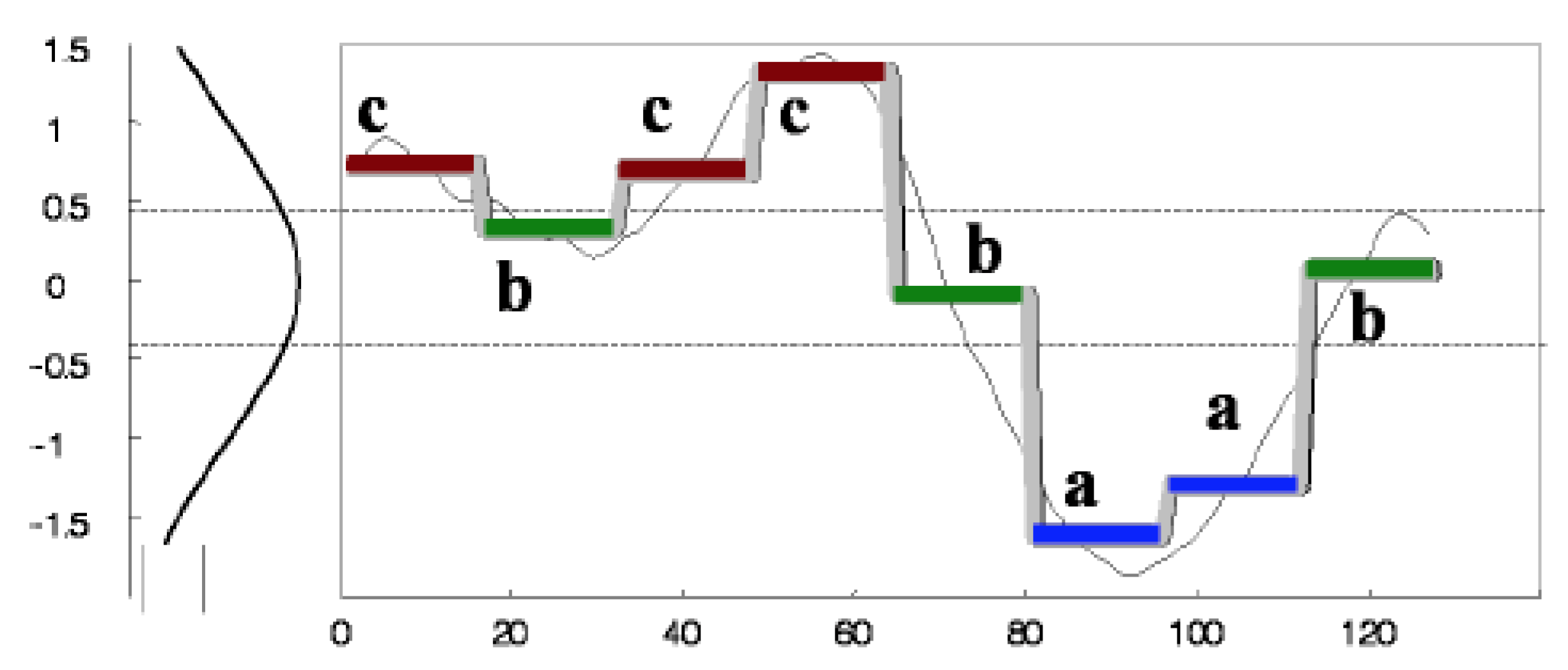
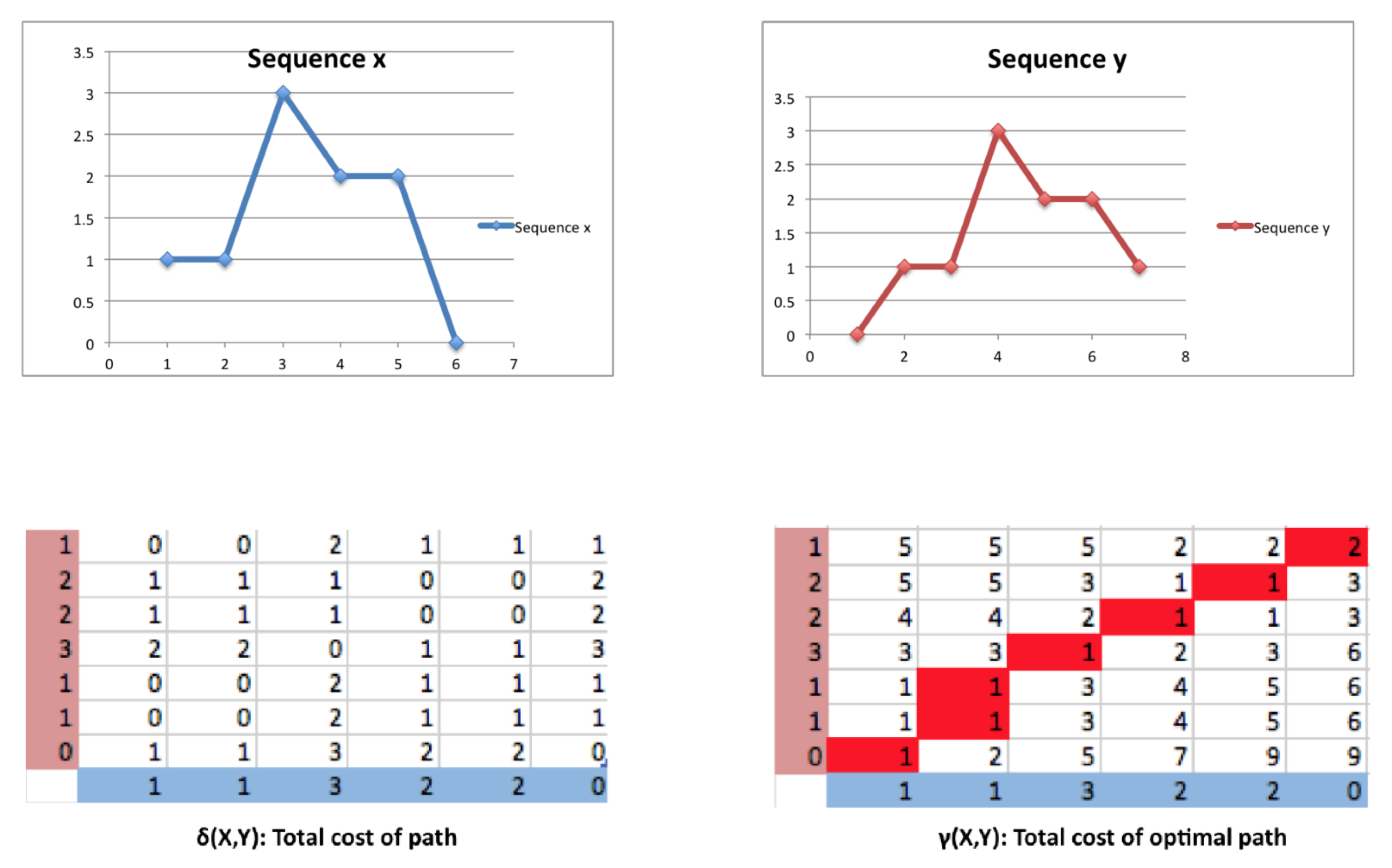
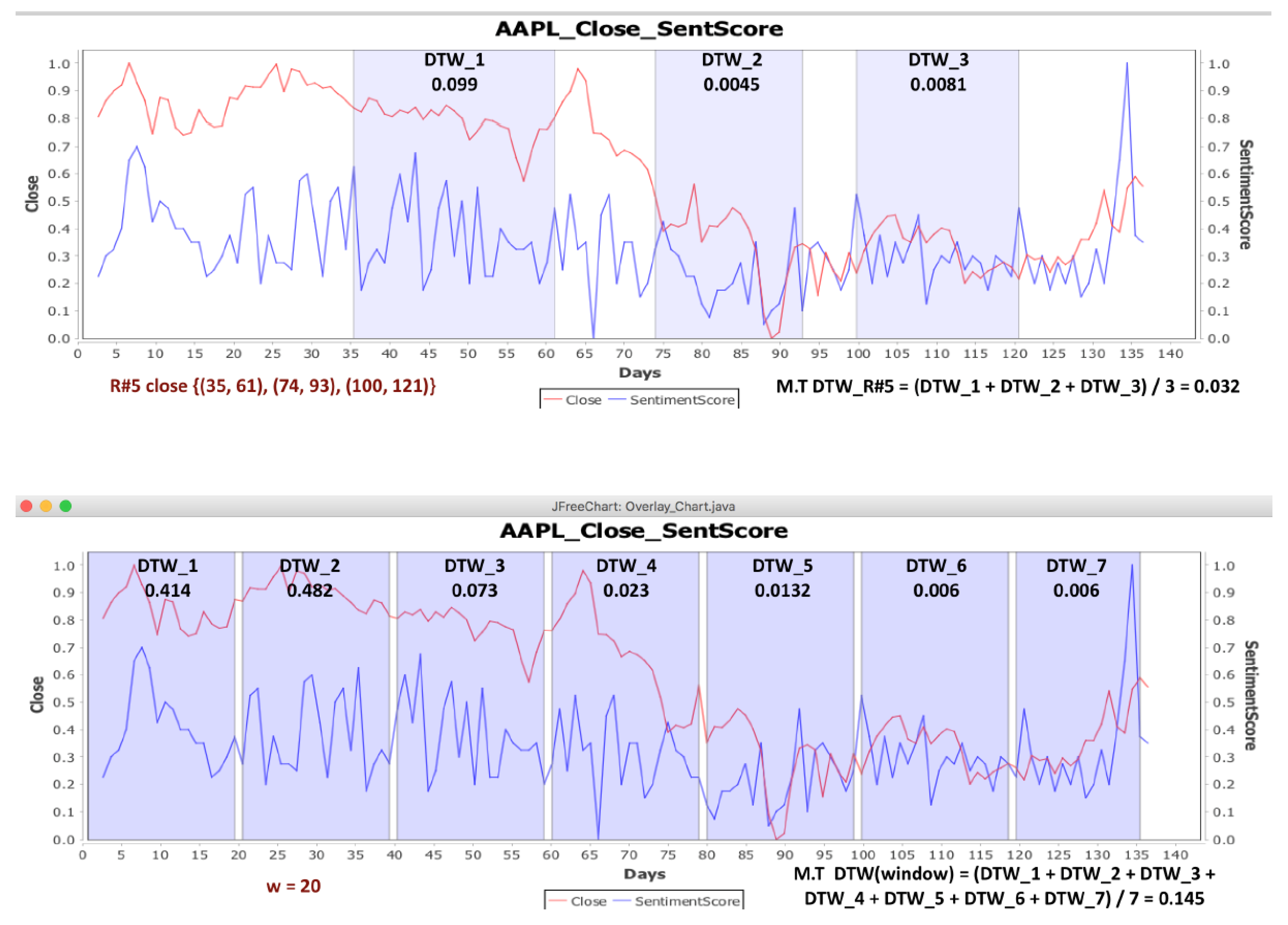
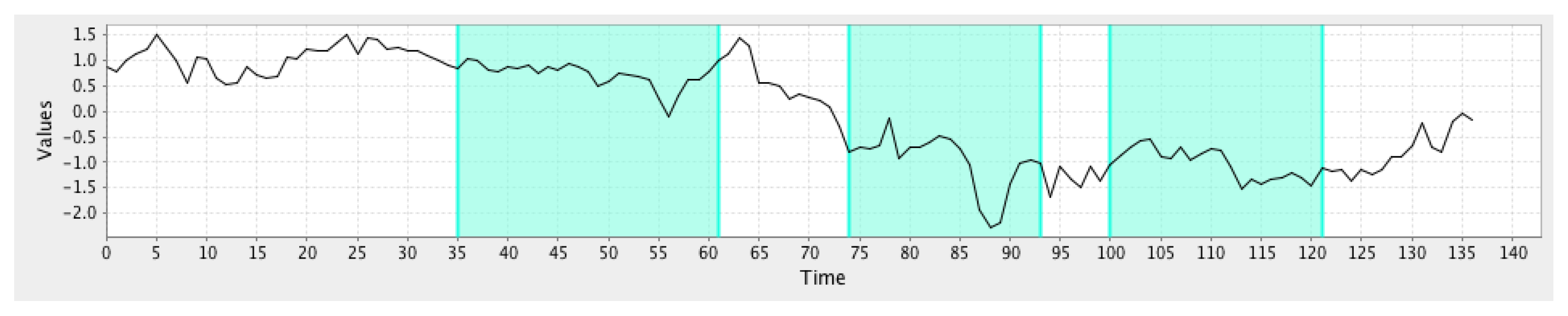
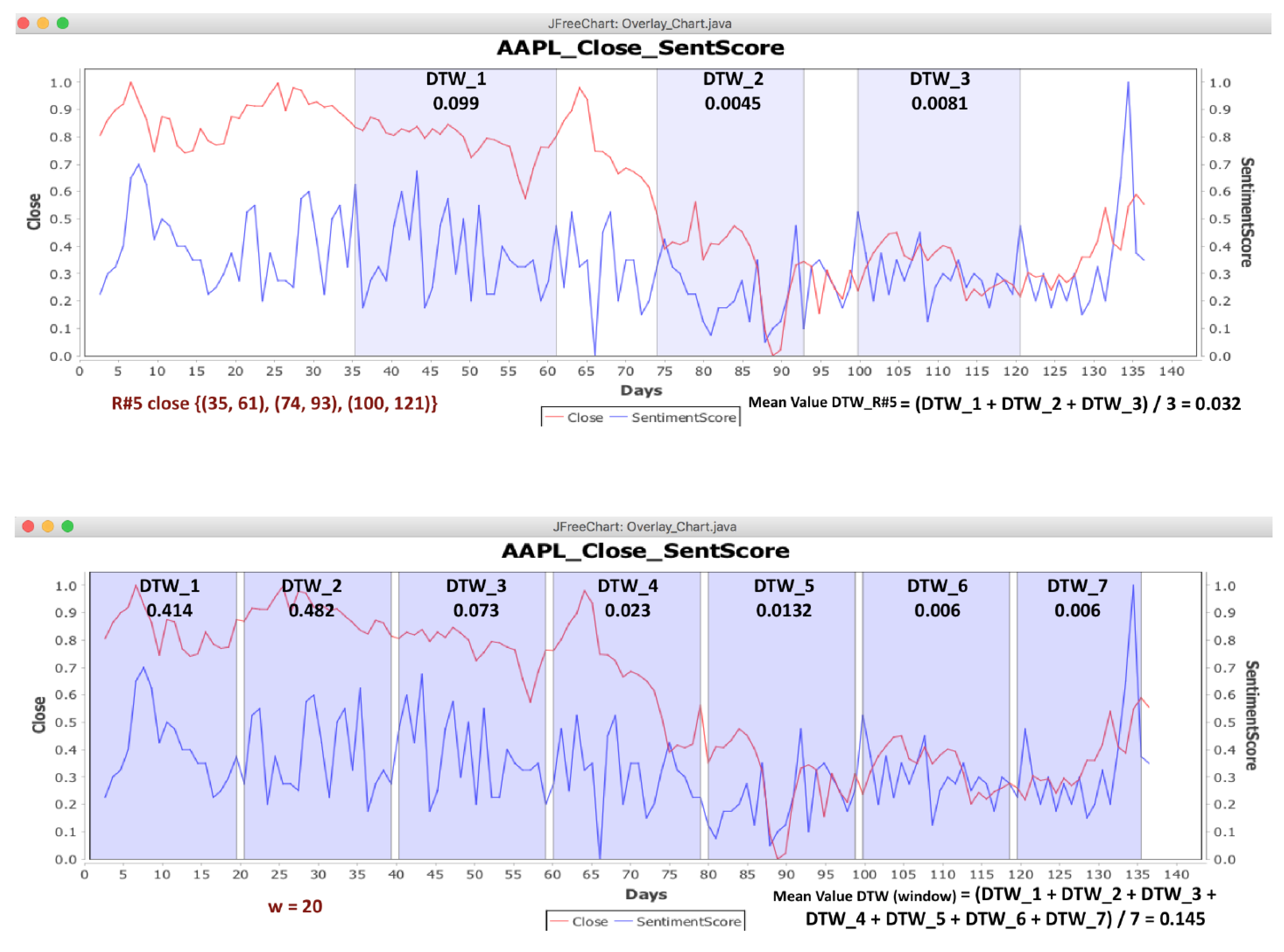
to use the DTW algorithm. First, for each of the five stocks (AAPL, GE, IBM, MSFT and ORCL), we measured the DTW distance between the close time series and the sentimentScore time series. We measured the DTW distance between the two time series at the intervals of close time series, where patterns were found via the GrammarViz 2.0 API, ±3 units. For each rule, we found the Mean Value (M.V.) of the DTW distance of intervals that compose this rule. Tables S11–S15 show the DTW distances for AAPL, GE, IBM, MSFT and ORCL, respectively.
Then, random windows of w length were selected for the time series. Thus, we compared the mean value of the DTW distance of each rule to the mean value of the DTW distance of the random windows. If the mean value of the DTW distance of rules was smaller than the mean value of the DTW distance of the random window, then there was a correlation between the time series at the intervals of rules where patterns were found in the close time series (Figure 6).
The two time series are considered to be similar when the value of their distance is close to zero. On the other hand, when the distance is closer to one, that means that there is difference between the two time series.
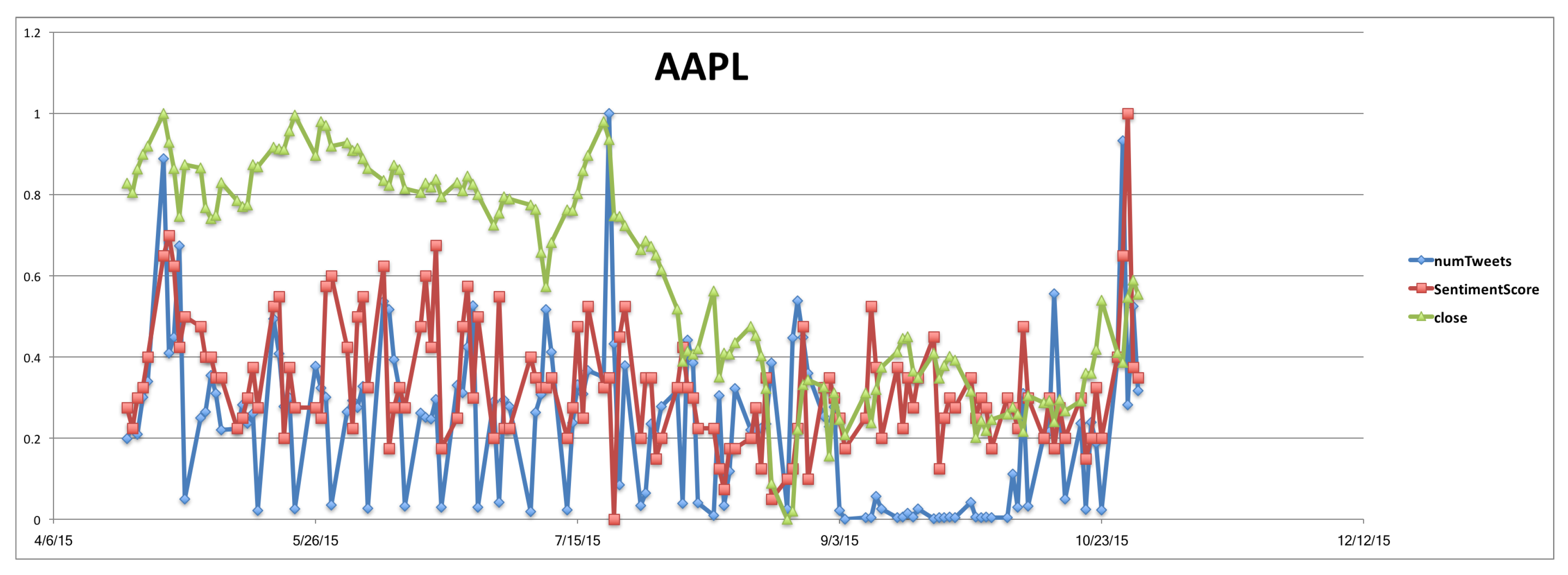
For example, we compared the mean value (M.V.) of the rules of the patterns that were found for AAPL company (stock) (Supplementary Material file, Table S11) with the mean value of the random windows. As seen, the mean value of the distance of the R # 1 rule is equal to 0.179, but in Table S16, the mean value of the random window for the AAPL stock is smaller than this of R # 1 rule. Thus, for the intervals of the rule R # 1 , we cannot say that there is a correlation between the two time series. On the other hand, for the rule R # 2 (Supplementary Material file, Table S11), the mean value of the distance is equal to 0.068. In Table S16, we will see that there are random windows for which their mean value is bigger than the mean value of R # 2 . This means that there is a correlation between the two time series in ((4, 21), (79, 98)) intervals of the R # 2 . In addition, Table S16 depicts the random windows that we have taken for the five companies (AAPL, GE, IBM, MSFT, ORCL).
Table S17 of the Supplementary Material file gives an overview of all the rules of the five companies where there is a correlation, i.e., a small DTW distance between the two time series. There are many rules with a small DTW distance, thus there is a correlation between close and sentimentScore time series (i.e., between closing price and news).
In order to check if there is a correlation between the time series of closing prices (close) and the number of tweets (numTweets), we followed the same steps as for the closing price and news. We measured the DTW distance between the close and the numTweets time series. Tables S18–S22 of the Supplementary Material file show the distances for each stock that were found via the DTW algorithm. For each rule, the mean value of the distances of intervals, which are composing the rule, is calculated. The process to find if there is a correlation between the two time series is the same as the process of the close and the sentimentScore time series. In more detail, we compared the mean value of rules with the mean value of the random windows. If the mean value of the rules is smaller than the mean value of the random windows, there is a correlation between the two time series. We observed that in this case, also, there are intervals (i.e., rules) with a very small distance with respect to the random intervals (Supplementary Material file, Table S23), which means that the close and numTweets time series are similar in these intervals; consequently, there is a correlation.
Table S24 of the Supplementary Material file gives an overview of all the rules of the five companies where there is a correlation, i.e., a small DTW distance between the two time series. There are many rules with a small DTW distance; thus, there is correlation between close and numTweets time series (i.e., between closing price and number of tweets).

5.5.1. Forecasting Methods and Models

Time series forecasting performance is usually evaluated upon training some model over a given period of time and then asking the model to forecast the future values for some given horizon. Provided that someone already knows the real values of the time series for the given horizon, it is straightforward to check the accuracy of the prediction by comparing them with the forecasting values.
Denoting a time series of interest as y t with N points and a forecast of it as f t , the resulting forecast error is given as e t = y t f t , f o r t = 1 , , N . Using this notation, the most common set of forecast evaluation statistics considered can be presented as below (Table 2).
Intuitively, RMSE and MAE focus on the forecasting accuracy; RMSE assigns a greater penalty on large forecast errors than the MAE, while the U 2 statistic focuses on the quality, which will take the value of one under the naive forecasting method. Values less than one indicate greater forecasting accuracy than the naive forecasting method, and values greater than one indicate the opposite.
According to the literature, the most frequently used methods for time series forecasting include Autoregressive Integrated Moving Average (ARIMA) [20,21], Linear Regression (LR) [22], the Generalized Linear Model (GLM) [22], Support Vector Machines (SVM) [23] and Artificial Neural Networks (ANN) [24].

ARIMA

There are two commonly-used linear time series models in the literature, i.e., Autoregressive (AR) and Moving Average (MA) models. Combining these two, the Autoregressive Integrated Moving Average (ARIMA) model has been proposed in the literature. In a similar way to regression, ARIMA uses independent variables to predict a dependent variable (the series variable). The name autoregressive implies that the series values from the past are used to predict the current series value. In other words, the autoregressive component of an ARIMA model uses the lagged values of the series variable, that is values from previous time points, as predictors of the current value of the series variable.

LR and GLM

LR can be used to fit a forecasting model to an observed dataset, consisting of values of the response and explanatory variables. Upon learning of such a model, often fitted using the least squares approach, if additional values of the explanatory variables are collected without the accompanying response value, the fitted model can be used to make a prediction of the response. GLM is a flexible generalization of ordinary LR that allows for response variables to have error distributions other than the normal (Gaussian) distribution.

SVM

Initially, SVM were mainly applied to pattern classification problems such as character recognition, face identification, text classification, etc. However, soon, researchers found wide applications in other domains as well, such as function approximation, regression and time series forecasting. SVM techniques are based on the structural risk minimization rule. The objective of SVM is to find a decision rule with good generalization capability through selecting some particular subset of training data called support vectors. In this method, a best possible separating hyperplane is constructed, upon nonlinearly mapping of the input space into a higher dimensional feature space. Thus, the quality and complexity of SVM solution is not directly dependent on the input space. Another important characteristic of SVM is that the training process is equivalent to solving a linearly inhibited quadratic programming problem.

ANN

The ANN approach has been endorsed as an alternative technique to time series forecasting and has achieved immense popularity in the last few years. The main objective of ANN is to build a model for mimicking the intelligence of the human brain in a machine. Similar to the processed followed by a human brain, ANN will try to identify predictabilities and patterns within the input data, learn from past knowledge and then provide accurate estimates on new, unobserved data. Despite the fact that the development of ANN was mainly biologically motivated, they have been applied in numerous domains, primarily for forecasting and classification purposes. The main characteristic of ANN is that it is a data-driven and self-adaptive in nature method. There is no need to specify a particular model form or to make any a priori statement about the statistical distribution of data. Therefore, the desired model is adaptively formed and based on the features presented from the data.
Despite the fact that ARIMA only supports univariate time series and therefore cannot cope with sentiment data from news or tweets, we initially carried out an evaluation of the aforementioned models upon only the closing price of each of the five stock indices, namely AAPL, GE, IBM, MSFT and ORCL. Data from each company were split into two subsets, i.e., a training set of the first 127 days and a test set of the remaining 10. Since all models are sensitive to internal parameters, such as p (order of the autoregressive model) and q (order of the moving average) for ARIMA, ϵ (learning rate) for the ANN, C (misclassification coefficient) for SVM, etc., we applied a grid search approach that optimized these parameters on the training set. This approach searched among various combinations of the parameters for the model that minimized the RMSE, using 10-fold cross-validation on the first 127 days. Therefore, we ensured that the last 10 days used as the test set would never be known to any of the above models. 
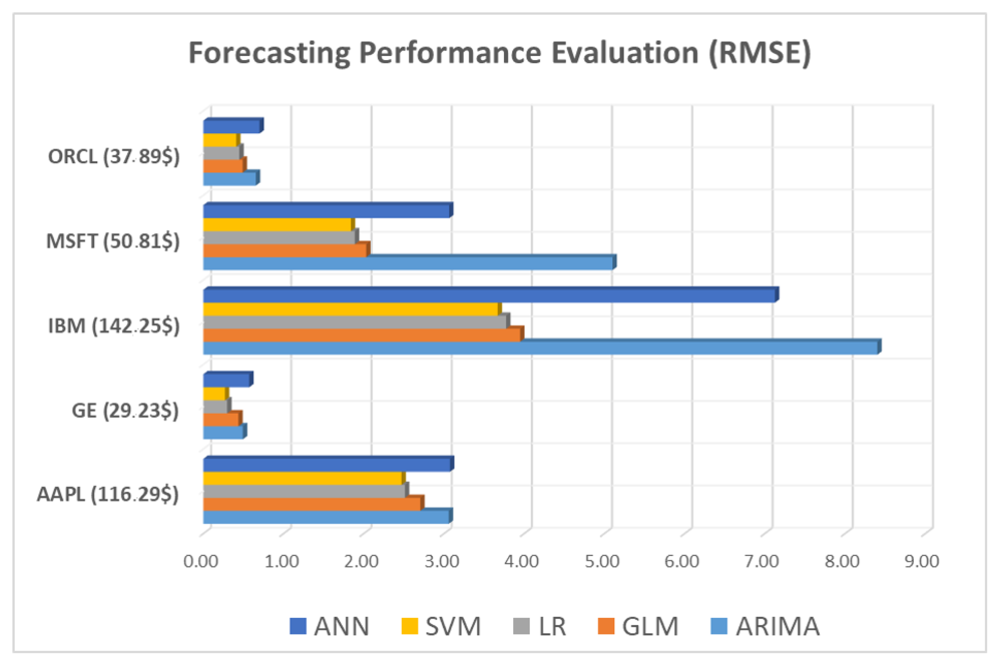
Figure 7 tabulates the performance of each model expressed in RMSE, for each stock. In the parenthesis next to the stock’s index, the average close price for the last 10 days test set is included.
As regards Theil’s U 2 decomposition metric, the results support our aforementioned claim about the superiority and robustness of SVM and LR, since as shown in Table 3, they present the lowest U 2 scores.
Based on the above, we only consider the first two superior models, i.e., SVM and LR, throughout the further experiments that would examine if news and tweets can improve the prediction of the closing price of the next day, especially when considering time periods that have been identified from the rule extraction phase.
Even though the obvious approach when comparing two forecasting models is to select the one that has the smaller error measurement based on one of the error measurements described above, we need to determine whether this difference is significant or basically due to the specific choice of data values in the sample. Therefore, each of the five forecasting models was compared to the others in terms of the Diebold–Mariano (DM) test [25].
Considering the null hypothesis to be as: “both forecasting model have the same accuracy”, the DM test returns two metrics, i.e., a p-value, denoting that the hypothesis holds when close to one or does not hold when close to zero, and DM-statistics, measuring the squared errors of the two models. Negative values show that the squared errors of the model listed first are lower than those of the model listed last.
For reasons of space economy, Table 4 tabulates the DM test between all models for the AAPL stock. The results for the other companies are almost identical to AAPL.
We could observe that based on both the p-values and DM-statistic metrics, LR and SVM can be considered as having almost the same accuracy, while all other pairs of comparisons do not follow this trend, with the small exception of the GLM method.

5.5.2. Can News and Tweets Improve the Prediction of the Next Closing Price?

In order to check if the sentiment score of the news and the number of tweets can improve the prediction of the next closing price, we examined the intervals in which there are patterns and at the same time have a small DTW distance, i.e., the rules that have a small DTW distance (Supplementary Material file, Table S25). If the sentiment score of news and the number of tweets on these rules help to improve the prediction, then the rules are more useful than the random intervals of days. Thus, the experiments to check if these rules improve the prediction of the next closing price were performed as follows:
  • the sentiment score of news
  • the number of tweets
  • both of them
Afterwards, we compared these rules against random intervals of time. In the random intervals of time, the improvement rates of the next closing price are calculated, again, by the sentiment score of news, the number of tweets and both of them.
The RapidMiner tool [26] was used for the experiments, and for the prediction, we used two methods of regression, linear regression and the SVM regression. Due to the fact that linear and SVM regression are two of the most popular algorithms in predictive modeling, we decided to perform our experiments by using these two methods. In addition, SVM is a rather robust method for forecasting. The prediction was based on the three previous days. Then, we compared the two methods to evaluate which gives better improvement rates. 
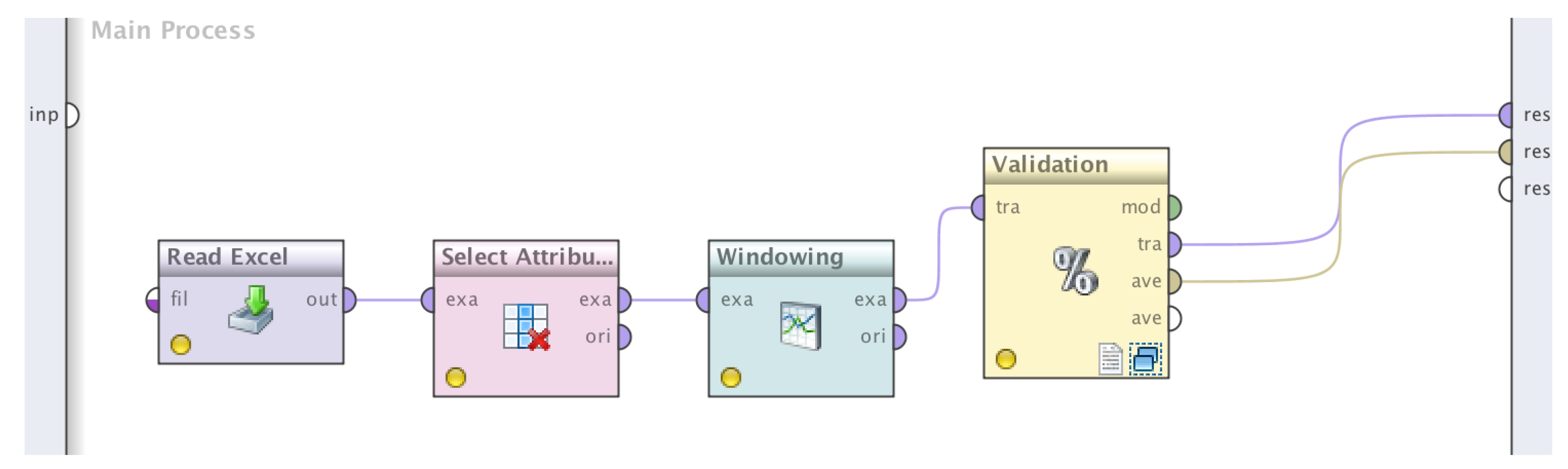
Figure 8 shows the basic process, which consisted of the following four processes in the RapidMiner tool.
The steps of the process in more detail:
  • This operator can be used to load data from Microsoft Excel spreadsheets. In our case, the excel file that will be loaded in the Rapid Miner tool has the following columns (attributes): date, close, volume, open, high, low, sentiment and tweets.
  • This operator selects which attributes of an ExampleSet should be kept and which attributes should be removed. This is used in cases when not all attributes of an ExampleSet are required; it helps to select required attributes. In our case, we selected the “date” as a filter of attributes, and we selected the option “invert selection” because we needed to filter a subset of attributes.
  • Windowing
    This operator transforms a given example set containing series data into a new example set containing single valued examples. For this purpose, windows with a specified window and step size are moved across the series, and the attribute value lying horizon values after the window end is used as a label that should be predicted. In simpler words, we select the step in order to make the prediction. We have chosen to predict the next closing price based on the three previous days.
  • This operator performs a cross-validation in order to estimate the statistical performance of a learning operator (usually on unseen datasets). It is mainly used to estimate how accurately a model (learned by a particular learning operator) will perform in practice. As previously explained, the two most accurate regression types were used for our experiments, i.e., linear regression and Support Vector Machines (SVM).
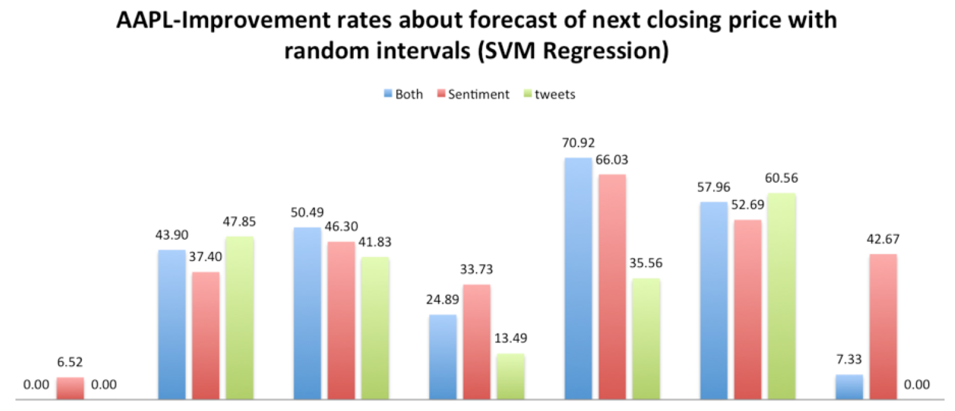
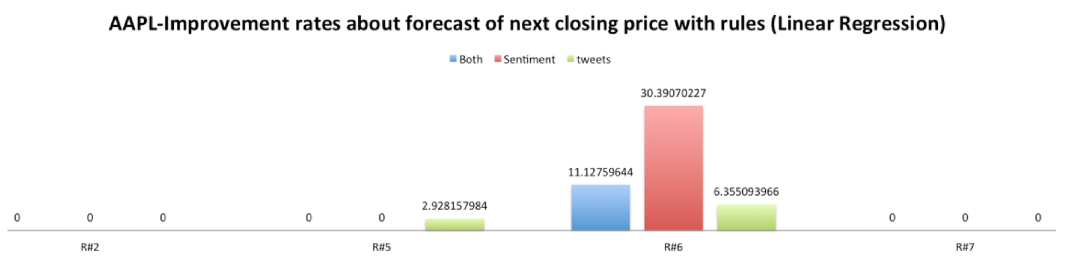
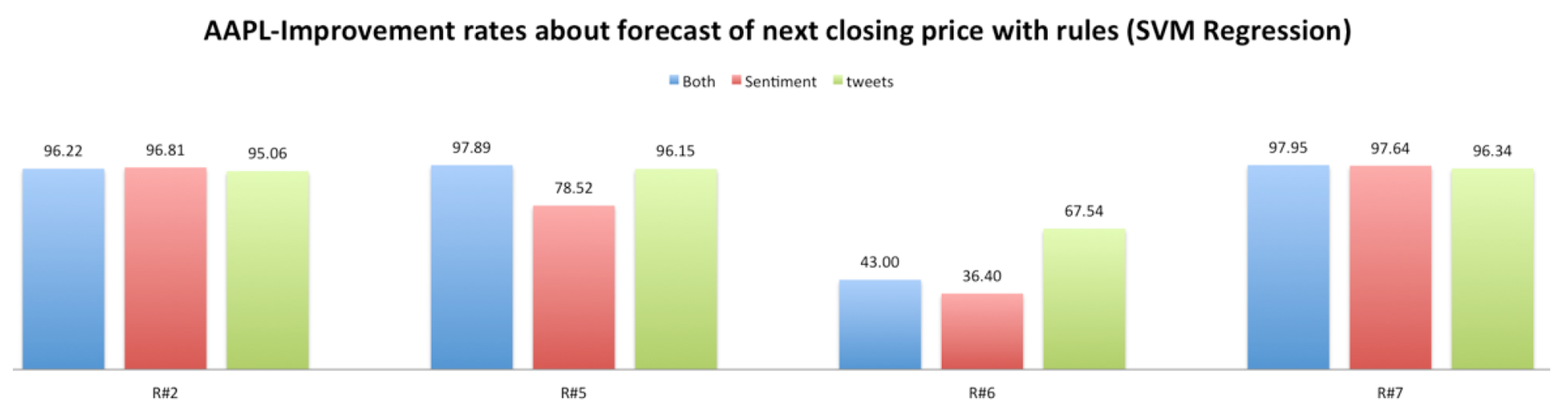
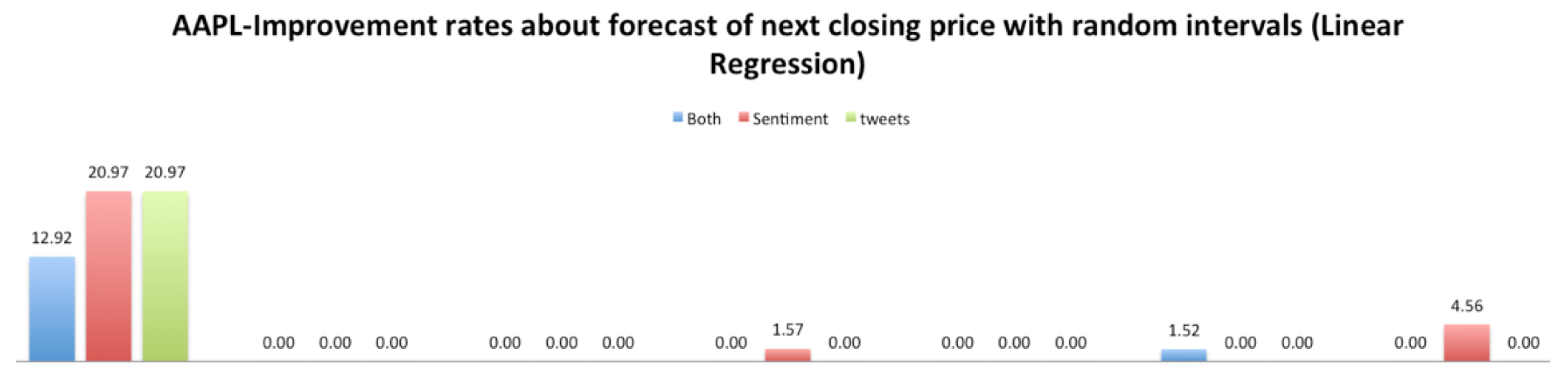
As we can see in Figure 9, Figure 10, Figure 11 and Figure 12, the improvement rates were better when we used the rules than the random intervals. Furthermore, using SVM regression, we have better results than with the linear regression. Similar results were found for the other four stocks, and in most cases, the rules improved the prediction of the next closing price. The improvements are depicted below in Table 5 and Table 6.

5.5.3. Results

We have also performed a DM-test to verify that the forecasting performance of SVM within the intervals denoted by the rules is superior to the outcome of the same method for random intervals. We used the dataset of both sentiments and tweets to conduct the evaluations for all stock prices. Again, the null hypothesis was considered to be that the two forecasting models (rule vs. random intervals) have equal accuracy.
Table 7 presents the p-value and DM-statistic metrics. Recall that when the p-value is close to zero, the null hypothesis is rejected. Furthermore, negative values of the DM-statistic depict that the squared errors of the model listed first (the rule-based intervals) are lower than those of the model listed last.
As seen from that table, for all companies, p-values are close to zero and the DM-statistic is negative, denoting that not only the null hypothesis does not hold, but the intervals identified by the rules have lower squared errors.
The fact that rules have been found in which the sentiment score, the tweets or both can improve the prediction is a very encouraging result for further future study.
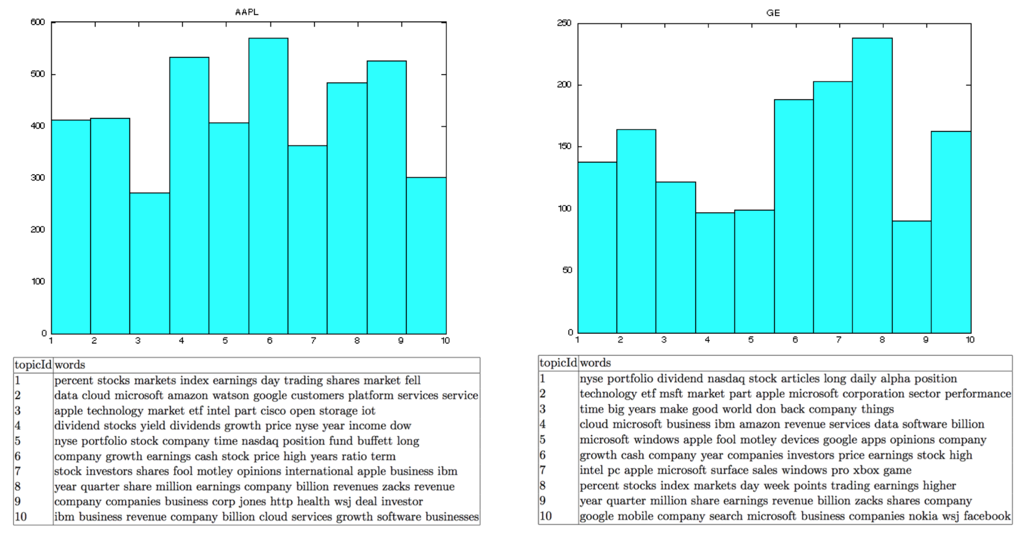
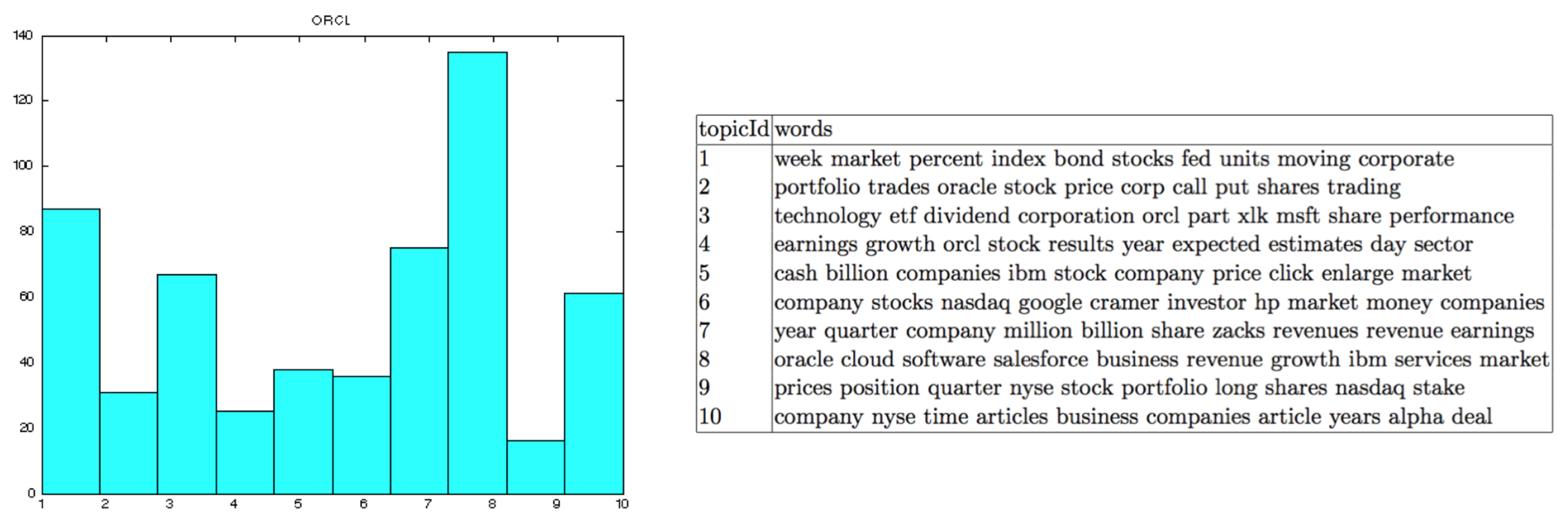
In Figure 13, Figure 14 and Figure 15, all texts have been clustered in topics, using the LDA algorithm. The latter could help to improve our method by incorporating a better filtering of news data by using the topic of each text. In other words, we could choose the texts that are more relevant to the stock market, based on the results of the topic modeling.

6. Shortcomings of the Study

Although our work has reached its aims, there are some limitations. First, this work was conducted on a small dataset. Therefore, the experiments need to be further elaborated in order to include more stock prices. Finally, the dataset of the news articles is not clustered in topics, and the texts could be more relevant to the stock market. Thus, the news articles need to be clustered in topics to improve our method by incorporating a better filtering of news data by using the topic of each text.

7. Conclusions

In this paper, we investigated and modeled the impact of technical analysis, news articles and Twitter on predicting the stock market value. We first studied the existence of a relation between the time series of the stock closing price and news articles and the stock closing price and tweets. Using the SAX method, we calculated the mean DTW distance between the time series; close-stentimentScore and close-numTweets in the period of ±3 days. We found that there is correlation between our time series. Secondly, we examined if the news and tweets can improve the prediction of the next stock closing price using the patterns that have been identified and the DTW distance. For our experiments concerning the prediction, we used two methods of regression: linear regression and SVM regression. The results obtained are very encouraging and show that the improvement rates are better when we use the rules than the random intervals. Furthermore, using the SVM regression, we achieved better results compared with the linear regression. Even though the experiments need to be further elaborated in order to include more stock prices, adjusted for average long turn trends, the proposed framework justified that the technical and sentiment data of different stocks result in the similar behavior of the forecasting model, which is encouraging. Nevertheless, this is a first approach to provide some evidence on the usefulness of the sources of information to the task at hand.
As future work, the method could be improved by incorporating a better filtering of news data and by discovering and using the topic of each text (i.e., using topic modeling).

Supplementary Materials

The following are available online at https://www.mdpi.com/1999-4893/11/11/181/s1.

Author Contributions

M.M. conceived of the idea. F.K.-K., M.M. and A.K. designed the experiments and F.K.-K. performed the experiments. F.K.-K., M.M. and A.K. analyzed the results, drafted the initial manuscript and revised the final manuscript.

Funding

This work has been partially supported by project PADGETS: FP7-ICT-2009.7.3 “ICT for Governance and Policy Modeling Policy Gadgets Mashing Underlying Group Knowledge in Web 2.0 Media”.

Conflicts of Interest

The authors declare no conflicts of interest.

References

  1. Technical-Analysis. The Trader’s Glossary of Technical Terms and Topics. Available online: http://www.traders.com (accessed on 10 August 2018).
  2. Anny, N.; Wai-Chee, F.A. Mining frequent episodes for relating financial events and stock trends. In Pacific-Asia Conference on Knowledge Discovery and Data Mining; Springer: Berlin/Heidelberg, Germany, 2003; pp. 27–39. [Google Scholar]
  3. Liu, Y.; Huang, X.; An, A.; Yu, X. ARSA: A sentiment-aware model for predicting sales performance using blogs. In Proceedings of the 2007 ACM 30th Annual International ACM SIGIR Conference on Research and Development in Information Retrieval, Amsterdam, The Netherlands, 23–27 July 2007; pp. 607–614. [Google Scholar]
  4. Jacob, B.; Ronen, F.; Shimon, K.; Matthew, R. Which News Moves Stock Prices? A Textual Analysis; National Bureau of Economic Research: Cambridge, MA, USA, January 2013. [Google Scholar]
  5. Roll, R. R2. J. Financ. 1988, 43, 541–566. Available online: https://doi.org/10.1111/j.1540-6261.1988.tb04591.x (accessed on 6 November 2018). [CrossRef]
  6. Ruiz Eduardo, J.; Hristidis, V.; Castillo, C.; Gionis, A.; Jaimes, A. Correlating financial time series with micro-blogging activity. In Proceedings of the 2012 ACM Fifth ACM International Conference on Web Search and Data Mining, Seattle, WA, USA, 8–12 February 2012; pp. 513–522. [Google Scholar]
  7. Mao, Y.; Wei, W.; Wang, B. Correlating SandP 500 stocks with Twitter data. In Proceedings of the 2012 ACM First ACM International Workshop on Hot Topics on Interdisciplinary Social Networks Research, Beijing, China, 12–16 August 2012; pp. 69–72. [Google Scholar]
  8. Xue, Z.; Hauke, F.; Gloor, P.A. Predicting stock market indicators through Twitter “I hope it is not as bad as I fear”. Procedia Soc. Behav. Sci. 2011, 26, 55–62. [Google Scholar]
  9. Robert, S.; Hsinchun, C. Textual analysis of stock market prediction using financial news articles. In Proceedings of the 2006 AMCIS Americas Conference on Information Systems, Acapulco, Mexico, 4–6 August 2006; Volume 185. [Google Scholar]
  10. Li, X.; Xie, H.; Chen, L.; Wang, J.; Deng, X. News impact on stock price return via sentiment analysis. Knowl. Based. Syst. 2014, 69, 14–23. [Google Scholar] [CrossRef]
  11. Carlo, S.; Alessandro, V. Wordnet Affect: An Affective Extension of Wordnet; Lrec: Lisbon, Portugal, 2004; pp. 1083–1086. [Google Scholar]
  12. Erik, C.; Daniel, O.; Dheeraj, R. SenticNet 3: A common and common-sense knowledge base for cognition-driven sentiment analysis. In Proceedings of the Twenty-Eighth AAAI Conference on Artificial Intelligence, Quebec City, QC, Canada, 27–31 July 2014. [Google Scholar]
  13. Stefano, B.; Andrea, E.; Fabrizio, S. Sentiwordnet 3.0: An Enhanced Lexical Resource for Sentiment Analysis and Opinion Mining; Lrec: Valletta, Malta, 2010; pp. 2200–2204. [Google Scholar]
  14. Text Analysis and Sentiment Polarity on FIFA World Cup 2014 Tweets. ACM SIGKDD 2005. Chicago, IL, USA. Available online: http://aylien.com/sentiment-analysis/ (accessed on 6 November 2018).
  15. Lin, J.; Eamonn, K.; Stefano, L.; Bill, C. A symbolic representation of time series, with implications for streaming algorithms. In Proceedings of the 8th ACM SIGMOD Workshop on Research Issues in Data Mining and Knowledge Discovery, San Diego, CA, USA, 13 June 2003; pp. 2–11. [Google Scholar]
  16. Berndt, D.J.; James, C. Using Dynamic Time Warping to Find Patterns in Time Series. 1994, pp. 359–370. Available online: https://www.aaai.org/Papers/Workshops/1994/WS-94-03/WS94-03-031.pdf (accessed on 25 October 2018).
  17. Lin, J.; Keogh, E.; Patel, P.; Lonardi, S. Finding Motifs in Time Series. In Proceedings of the 8th ACM International Conference on KDD 2nd Workshop on Temporal Data Mining, Riverside, CA, USA, 23–26 July 2002; pp. 53–68. [Google Scholar]
  18. Senin, P.; Lin, J.; Wang, X.; Oates, T.; Gandhi, S.; Boedihardjo, P.A.; Chen, C.; Frankenstein, S.; Lerner, M. Grammarviz 2.0: A tool for grammar-based pattern discovery in time series. In Joint European Conference on Machine Learning and Knowledge Discovery in Databases; Springer: Berlin/Heidelberg, Germany, 2014; pp. 468–472. [Google Scholar]
  19. Bliemel, F. Theil’s forecast accuracy coefficient: A clarification. J. Mark. Res. 1973, 10, 444–446. [Google Scholar] [CrossRef]
  20. Jacobs, W.; Souza, A.M.; Zanini, R.R. Combination of Box-Jenkins and MLP/RNA Models for Forecasting Combining Forecasting of Box-Jenkins. IEEE Lat. Am. Trans. 2016, 14, 1870–1878. [Google Scholar] [CrossRef]
  21. Vagropoulos, S.I.; Chouliaras, G.I.; Kardakos, E.G.; Simoglou, C.K.; Bakirtzis, A.G. Comparison of SARIMAX, SARIMA, Modified SARIMA and ANN-based Models for short-term PV generation forecasting. In Proceedings of the IEEE International Energy Conference (ENERGYCON), Leuven, Belgium, 4–8 April 2016. [Google Scholar]
  22. Stock, J.H.; Watson, M. Combination Forecasts of Output Growth in a Seven-Country Dataset. J. Forecast. 2004, 23, 405–430. [Google Scholar] [CrossRef]
  23. Cao, L.J.; Tay, F.E.H. Financial forecasting using support vector machines. Neural Comput. Appl. 2001, 10, 184–192. [Google Scholar] [CrossRef]
  24. Guresen, E.; Kayakutlu, G.; Daim, T.U. Using Artificial Neural Network Models in Stock Market Prediction. Expert Syst. Appl. 2011, 38, 10389–10397. [Google Scholar] [CrossRef]
  25. Diebold, F.X. Comparing predictive accuracy, twenty years later: A personal perspective on the use and abuse of Diebold–Mariano tests. J. Bus. Econ. Stat. 2015, 33, 1. [Google Scholar] [CrossRef]
  26. YALE: Rapid Prototyping for Complex Data Mining Tasks. KDD 2006. Philadelphia, Pennsylvania, USA. Available online: https://rapidminer.com/ (accessed on 6 November 2018).
Figure 1. Example Symbolic Aggregate Approximation (SAX) method to take a symbolic representation of a time series. Dimensionality reduction via Piecewise Aggregate Approximation (PAA). The symbolic representation is: baabccbc [15].
Algorithms 11 00181 g001
Figure 2. Example of the similarity comparison of two sequences using DTW. The δ distance measures the distance between two points in the time series. γ is the cumulative distance for each point. The closer to the diagonal the warping path is located, the more similar the two sequences are.
Algorithms 11 00181 g002
Figure 3. Testing the validity of a rule against random windows.
Algorithms 11 00181 g003
Figure 4. Time series of close, sentimentScore and numTweets about AAPL. Normalization into [0, 1] interval.
Algorithms 11 00181 g004
Figure 5. Rule R # 5 from AAPL close time series, as illustrated by GrammarViz 2.0. The frequency of the pattern is three times on intervals [35, 61], [74, 93] and [100, 121]. Rule R # 5 represents these three intervals.
Algorithms 11 00181 g005
Figure 6. If mean value DTW (R) < mean value DTW (w), where R: rule, w: window (random window size), then there exists a correlation between the two time series.
Algorithms 11 00181 g006
Figure 7. SVM and LR are outperforming all other models, with ARIMA and ANN having significantly worse performance.
Algorithms 11 00181 g007
Figure 8. The basic process in the RapidMiner tool.
Algorithms 11 00181 g008
Figure 9. Improvement rates (expressed in %) of pattern intervals (rules) about AAPL by using linear regression.
Algorithms 11 00181 g009
Figure 10. Improvement rates (expressed in %) of pattern intervals (rules) about AAPL by using SVM regression.
Algorithms 11 00181 g010
Figure 11. Improvement rates (expressed in %) at random intervals about AAPL by using linear regression.
Algorithms 11 00181 g011
Figure 12. Improvement rates (expressed in %) at random intervals about AAPL by using SVM regression.
Algorithms 11 00181 g012
Figure 13. Topic modeling for AAPL and GE stocks. The y-axis represents the number of texts in each topic, and the x-axis represents the topicId.
Algorithms 11 00181 g013
Figure 14. Topic modeling for IBM and MSFT stocks. The y-axis represents the number of texts in each topic, and the x-axis represents the topicId.
Algorithms 11 00181 g014
Figure 15. Topic modeling for ORCL stock. The y-axis represents the number of texts in each topic, and the x-axis represents the topicId.
Algorithms 11 00181 g015
Table 1. Total data for 137 days (20 April 2015 to 30 October 2015).
AAPLGEIBMMSFTORCL
Number of news4282150615492577575
Number of tweets310,50346,23756,80467,10716,494
Table 2. The most common set of forecast evaluation statistics.
Root Mean Squared Error (RMSE) R M S E = i = 1 N e i 2 N
Mean Absolute Error (MAE) M S E = i = 1 N e i N
Theil’s U 2 Decomposition 1 U 2 = i = 1 N 1 f i + 1 y i + 1 y i 2 N i = 1 N 1 y i + 1 y i y i 2 N
As U 1 has some serious disadvantages (see Bliemel 1973 [19]), it is recommended in the literature to use U 2 .
Table 3. Theil’s U 2 decomposition results for the different algorithms and stocks.
Theil U Decomposition
Stock (Avg. Price in US$)ARIMAGLMLMSVMANN
AAPL (116.29 $)0.02630.02050.02170.02110.0263
GE (29.23 $)0.01070.01490.01020.01030.0195
IBM (142.25 $)0.05910.02700.02670.02640.0504
MSFT (50.81 $)0.04960.03370.03160.03160.0424
ORCL (37.89 $)0.01460.01190.01180.01170.0184
Table 4. Diebold–Mariano (DM)-test results on AAPL for all five forecasting models, carried out in pairs. Green colors represent high p-values, while red corresponds to cases where the null hypothesis is rejected due to almost zero p-values.
Null Hypothesis: Both Forecasts Have the Same Accuracy
p-valueARIMAGLMLRSVMANN
ARIMA 0.60670.65060.62800.5403
GLM 0.81320.91980.0086
LR 0.96360.0069
SVM 0.0076
ANN
DM-statisticARIMAGLMLRSVMANN
ARIMA 0.53570.47040.5038−0.6397
GLM 0.14420.0520−3.4563
LR 0.0473−3.6067
SVM −3.5415
ANN
Table 5. The improvement rates of the next closing price of the five companies using rules (in RapidMiner).
Sentiment and TweetsSentiment OnlyTweets Only
APPL Linear
R#2000
R#5002.93
R#611.1330.396.36
R#7000
APPL SVM
R#296.2296.8195.06
R#597.8978.5296.15
R#643.0036.4067.54
R#797.9597.6496.34
GE Linear
R#40.000.540.00
R#50.001.210.00
R#60.000.000.00
R#722.5225.740.00
GE SVM
R#483.1870.2565.67
R#599.7799.6699.61
R#651.0152.7855.37
R#745.6641.6832.28
IBM Linear
R#40.000.890.00
R#533.411.0037.61
R#60.000.000.00
R#70.000.000.00
IBM SVM
R#498.5385.6993.56
R#588.1390.0675.38
R#690.1990.5977.66
R#70.000.000.00
MSFT Linear
R#10.000.000.00
R#20.000.000.00
R#313.7112.8214.16
R#40.002.520.00
MSFT SVM
R#171.7664.360.00
R#234.4525.0727.95
R#37.837.410.00
R#476.7673.0965.78
ORCL Linear
R#50.000.000.00
R#60.0012.6017.26
R#75.120.0026.40
ORCL SVM
R#592.9124.6388.53
R#60.000.000.00
R#744.7512.350.00
Table 6. The improvement rates of the next closing price of the five companies using random intervals, without using rules (in RapidMiner).
Sentiment and TweetsSentiment OnlyTweets Only
APPL Linear
Random Interval #112.9220.9720.97
Random Interval #20.000.000.00
Random Interval #30.000.000.00
Random Interval #40.001.570.00
Random Interval #50.000.000.00
Random Interval #61.520.000.00
Random Interval #70.004.560.00
APPL SVM
Random Interval #10.006.520.00
Random Interval #243.9037.4047.85
Random Interval #350.4946.3041.83
Random Interval #424.8933.7313.49
Random Interval #570.9266.0335.56
Random Interval #657.9652.6960.56
Random Interval #77.3342.670.00
GE Linear
Random Interval #126.9426.9426.94
Random Interval #20.000.000.00
Random Interval #30.780.000.00
Random Interval #40.000.000.00
Random Interval #50.000.000.00
Random Interval #60.000.005.95
GE SVM
Random Interval #133.3327.2421.51
Random Interval #247.0437.5739.05
Random Interval #364.5570.3061.59
Random Interval #445.210.0039.32
Random Interval #525.040.0024.40
Random Interval #673.2770.6852.27
IBM Linear
Random Interval #10.000.000.00
Random Interval #21.100.000.00
Random Interval #30.0030.3130.31
Random Interval #46.952.6614.87
Random Interval #537.1639.0038.43
Random Interval #660.8860.8860.88
Random Interval #75.145.145.14
IBM SVM
Random Interval #145.4556.350.00
Random Interval #225.3225.5324.20
Random Interval #349.1526.1050.07
Random Interval #449.5761.3915.28
Random Interval #566.1026.1640.78
Random Interval #641.5512.8321.00
Random Interval #76.0330.800.00
MSFT Linear
Random Interval #172.9874.5774.57
Random Interval #225.1327.2627.26
Random Interval #357.9057.4957.90
Random Interval #465.3265.3265.32
Random Interval #50.3014.5614.56
Random Interval #617.863.9717.86
Random Interval #740.6342.0742.71
MSFT SVM
Random Interval #121.5933.897.25
Random Interval #259.4554.1050.23
Random Interval #320.0357.340.00
Random Interval #439.6451.1327.63
Random Interval #545.4734.484.25
Random Interval #622.4522.5410.11
Random Interval #791.5567.4092.20
ORCL Linear
Random Interval #167.8969.3969.39
Random Interval #20.0013.290.00
Random Interval #30.000.000.00
Random Interval #40.004.774.77
Random Interval #558.3458.3458.34
Random Interval #60.000.000.00
Random Interval #714.6330.2330.02
ORCL SVM
Random Interval #10.0019.610.00
Random Interval #260.2356.8720.32
Random Interval #350.800.0028.25
Random Interval #460.2462.0638.49
Random Interval #576.9273.7518.81
Random Interval #60.000.000.00
Random Interval #754.7549.1952.59
Table 7. DM-test between two forecasting models, based on SVM and using sentiments and tweets as additional features. The leftmost model is the one considering the intervals denoted by rules, while the rightmost represents the model of random intervals.
Null Hypothesis: Both Forecasts Have the Same Accuracy
Company IndexRules vs. Random Intervals
p-ValueDM Statistic
AAPL (116.29 $)0.1107−1.6839
GE (29.23 $)0.149−1.5968
IBM (142.25 $)0.081−2.2125
MSFT (50.81 $)0.09359−2.4001
ORCL (37.89 $)0.1367−1.5357

