1. Introduction
Intersection is one of the key elements of a modern traffic system. A great deal of time was wasted to wait for green lights, which brought huge economic losses [
1]. Traffic light is a conventional method to control traffic flows at intersections. Generally, the traffic lights with several signal phases are applied to coordinate conflicting traffic flows. While due to the limitations of traffic lights (i.e., the minimum and maximum green times), an approaching vehicle may have to spend some extra time for green lights even there are no potential collisions. These limitations not only decrease traffic efficiency but also cost unnecessary time of passengers.
In recent years, the Dedicated Short Range Communication (DSRC) technology has greatly facilitated the vehicle-to-vehicle and vehicle-to-infrastructure communication [
2,
3,
4,
5,
6,
7]. Based on DSRC, autonomous vehicles can be connected and share their information with other vehicles and infrastructures. Thus, CAVs can be coordinated simultaneously to improve traffic efficiency [
8]. Autonomous intersection, which is designed based on DSRC and CAVs, has drawn much attention around the world. A variety of algorithms for the management of an isolated autonomous intersection have been proposed to improve traffic efficiency without traffic lights.
According to the method used to coordinate approaching CAVs, the previous algorithms can be classified as global-trajectory-optimization based algorithms and non-global-trajectory-optimization based algorithms. For the global-trajectory-optimization based algorithms, the decision variables of the trajectories of many CAVs (at least including all CAVs in collision zones) are used to construct an optimization problem. These trajectories are optimized simultaneously using iteration calculation to determine the trajectories of these CAVs. For the no-global-trajectory-optimization based algorithms, there is no such an optimization problem. The permissions of CAVs to pass an intersection are determined by a predefined policy.
The global-trajectory-optimization based algorithms mainly include model predictive control [
9], genetic algorithm [
10], mix-integer non-linear programming [
11], mix-integer linear programming [
12,
13], integer linear programming [
14], linear programming [
8], etc. Using optimization, these algorithms can plan the trajectories of the CAVs at an intersection simultaneously to improve traffic efficiency. The main advantage of these algorithms is that the optimal calculation can be used to find an optimal or a local optimal solution for intersection management. Thus, theoretically, these algorithms show better performance than the non-global-trajectory-optimization-based algorithms. The major disadvantage of these algorithms is the high requirement for calculation. Due to the coupling of vehicle trajectories, these algorithms have to simultaneously control all CAVs at an intersection (at least within a certain range including all conflict zones), which leads to a high requirement for calculation from two aspects. First, the count of decision variables of optimal calculation increases with the count of CAVs, which aggravates the calculation burden. Second, even the trajectories of all CAVs at collision zones have been planned, these trajectories have to be planned again when a new approaching CAV is found. Thus, the trajectory of a CAV may be planned again and again, which further increases the high requirement for calculation.
The non-global-trajectory-optimization based algorithms mainly include cooperative adaptive cruise control [
15,
16], multi-agent [
1,
17], priorities and brake-safe control based algorithm [
18], auction [
19] (or market [
20]) based algorithm, buffer-assignment mechanism algorithm [
21], platoon based algorithm [
22], slots preassigning [
23], virtual traffic light [
24], and the combination of these algorithms [
25], etc. These algorithms can improve traffic efficiency by coordinating the orders of CAVs to pass intersections. The main advantage of these algorithms is the low computation burden. Thus, they can be easily applied for the intersections with a large number of CAVs. The disadvantage is that there is only one candidate trajectory for a CAV during a control circle. If there are potential collisions for a CAV, the CAV will have to slow down or stop to wait for a possible permission next control circle. Thus, there are still some potentials to improve traffic efficiency if more trajectories are designed and compared in a control circle.
Aiming to enhance traffic efficiency, a VB algorithm is proposed for the management of an isolated autonomous intersection. The proposed algorithm is divided into an offline algorithm and an online algorithm. By the proposed algorithm, most of the calculation caused by the coupling of vehicle trajectories can be done offline. There is no optimization problem to calculate the trajectories of all CAVs simultaneously in the VB algorithm. Thus, the VB algorithm is a no-global-trajectory-optimization based algorithm. Compared with previous no-global-trajectory-optimization based algorithms, the main advantage of the proposed algorithm is that, there are several candidate trajectories can be chose for a CAV to pass an intersection in a control circle. Thus, there are more opportunities for an approaching CAV to get a permission to pass an intersection. By contrast, for previous no-global-trajectory-optimization based algorithms, in a control circle, there is only one candidate trajectory can be used for an approaching CAV.
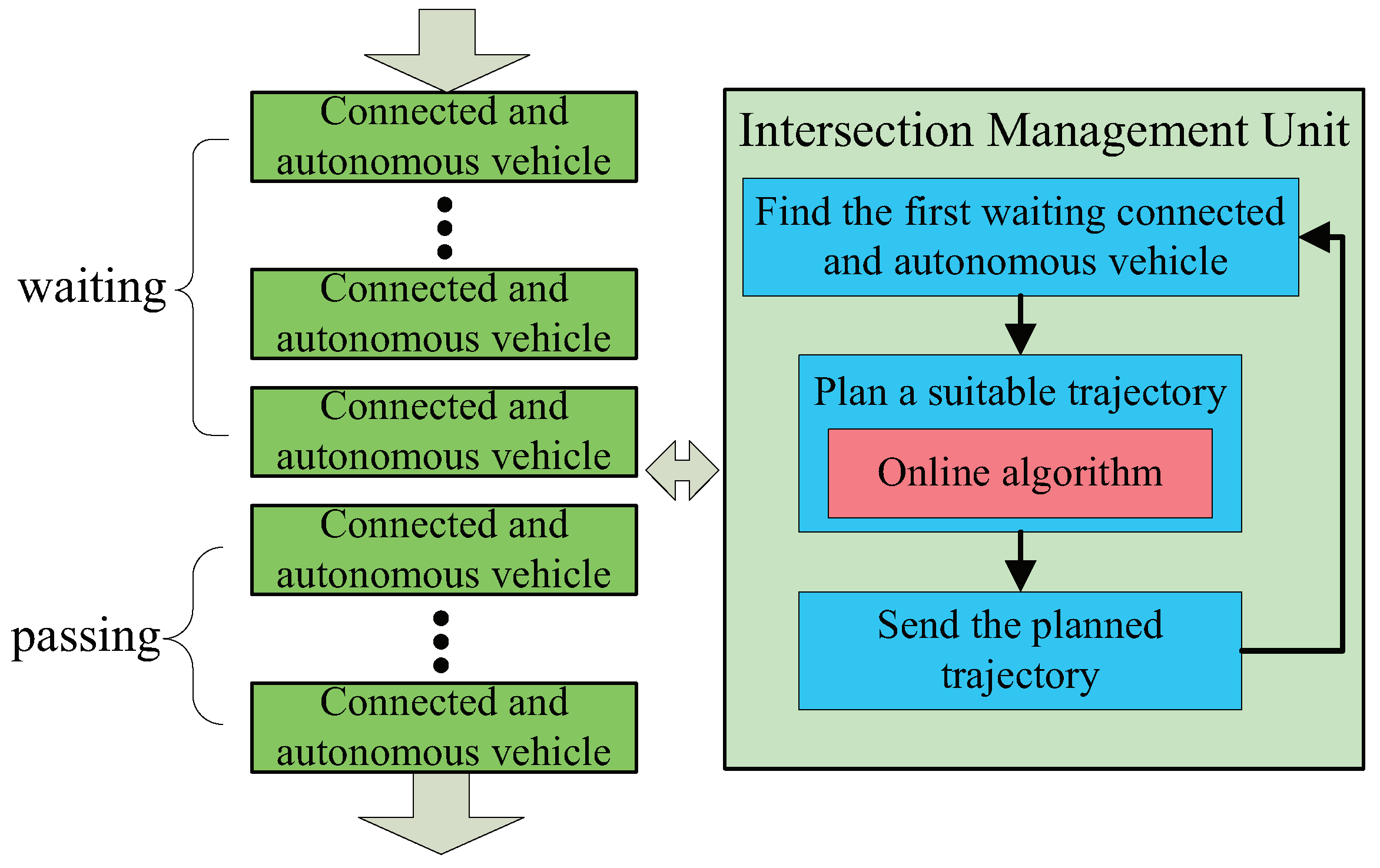
As shown in
Figure 1, the proposed VB algorithm consists of an online algorithm and an offline algorithm. As indicated by the name, the offline algorithm is used before the online application of the algorithm. The offline algorithm is comprised of VBs modeling and collision checking. By the method of VBs modeling, the considered intersection is modeled as several VBs. There are several VGs that fixed on each VB. The collision relations among these VGs can be obtained by collision checking. The online algorithm is used for the online application of the VB algorithm, which is designed based on the principle of “first-in-first-service” [
1]. The online algorithm consists of VG selecting and trajectory planning. Several suitable VGs can be obtained by the method of VG selecting. By the trajectory planning method, the most suitable VG and the collision free trajectory can be found for each approaching CAV. Following the planned trajectory, an approaching CAV can pass an intersection without collisions.
The remainders of the paper are organized as follows: In
Section 2, the problem of the considered intersection management is illustrated. In
Section 3, several basic conceptions of the VB algorithm are introduced, which lay the foundation of this algorithm. In
Section 4, the method to obtain the collision relation among the VGs in different VBs is proposed. In
Section 5, the initial ideal of VB algorithm is discussed, which provides a simple demonstration of the VB algorithm. In
Section 6, the VB algorithm designed for actual application is presented. In
Section 7, the numerical simulations of the VB algorithm are conducted to demonstrate the effectiveness of this algorithm. At last conclusion is given in
Section 8.
4. Collision Checking of Virtual Belts
In this section, the method to find the collision relation among the VGs of different VBs is shown. In certain condition, a very interesting phenomenon is that some VGs never collide with each other and some always collide with each other in each time circle.
4.1. Collision Checking between Virtual Grids
Consider two uniform VGs (
and
).
is born at
and
is born at
. Depending on the VPs and the born times of these VGs. During the time of (
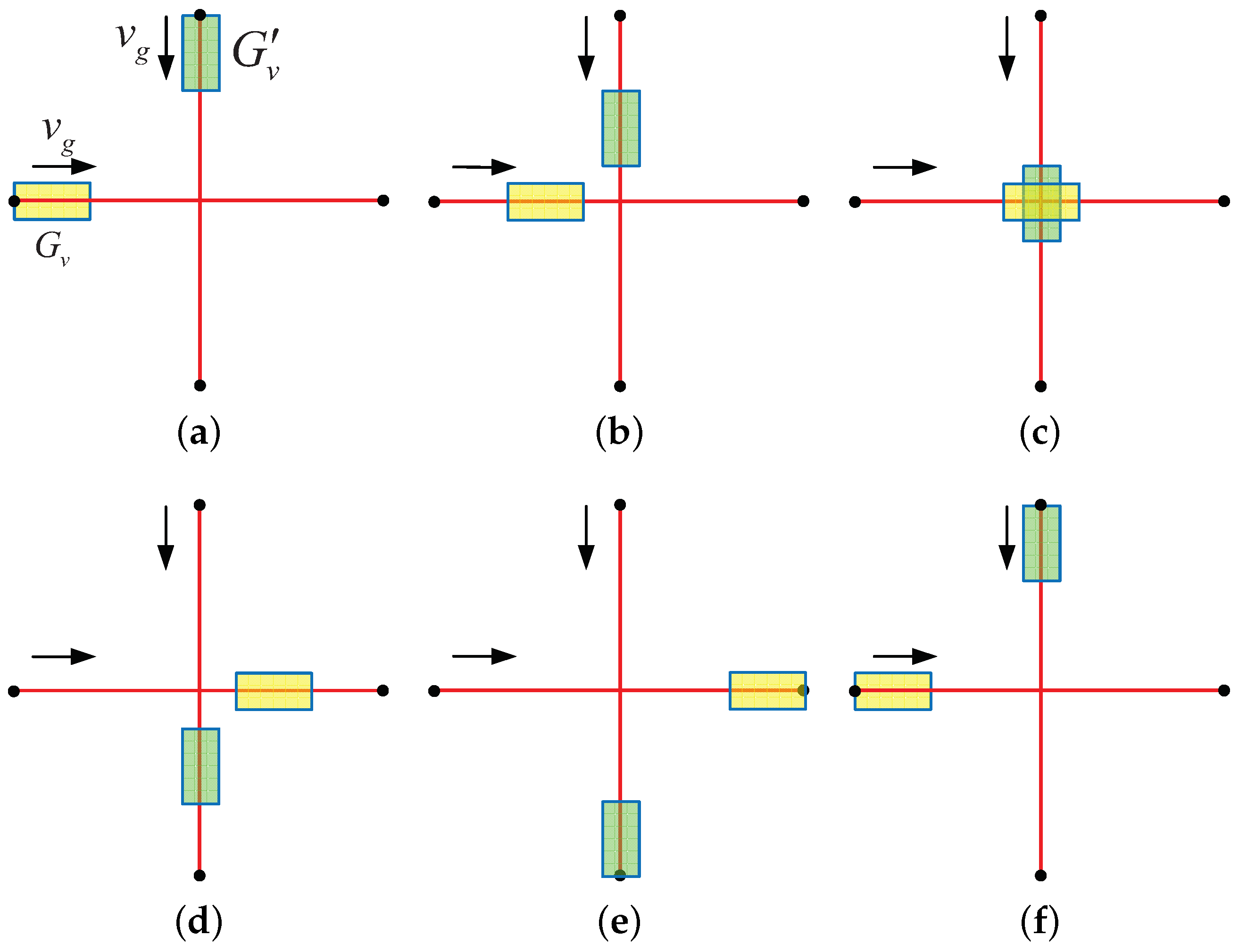
), there are only two possible results of collision checking between the two VGs. The first one is that
collides with
in a certain time as plotted in
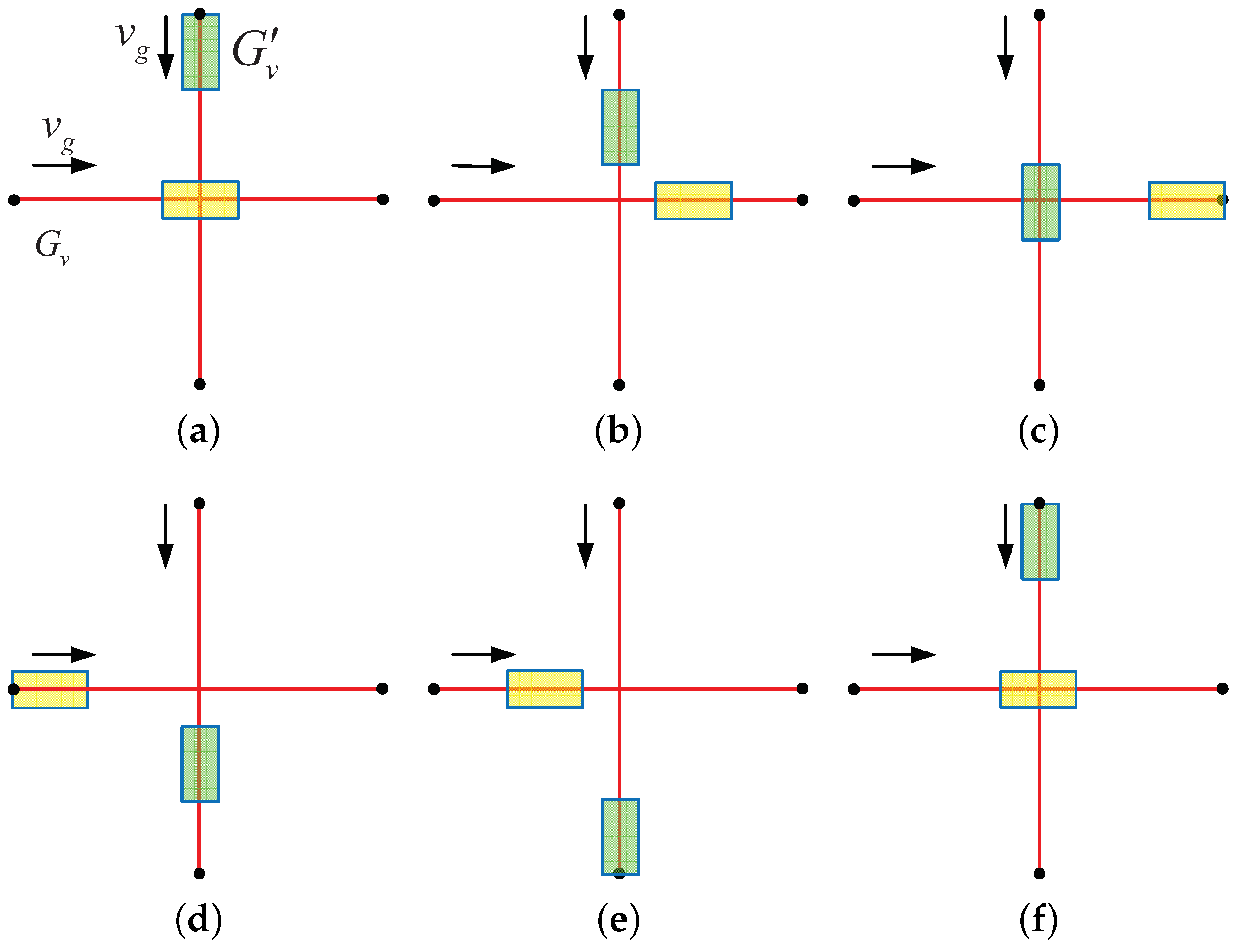
Figure 8. The second one is that
never collides with
as shown in
Figure 9.
These VGs move along the corresponding VPs with the same speed. If does not collide with during the time range of (, ), then will not collided with at the time range of (, ). Consequently, it can be deduced that and will not collide forever. Similarly, if collides with during the time range of (, ), then will collide with at each time circle in future. In another word, the future collision between two uniform VGs can be predicted based the result of collision checking in a time circle.
The collision checking algorithm for two uniform VGs is shown in Algorithm 1.
| Algorithm 1 Collision checking of two VGs. |
Input: two VGs ( and )
Output: whether two VGs will collide with each other in the future- 1:
Initial the positions of and - 2:
Divide the time circle (, ) into small enough segments: - 3:
fort in do - 4:
Calculate the positions of and at the time of t; - 5:
if and collide with each other then - 6:
return true - 7:
end if - 8:
end for - 9:
return false
|
If collides with in a time circle, is called a CVG of . The total CVGs of a VG is defined as the CVGR of the VG. CVGR provides a simple but effective method to record the collisions among VGs. As all VGs repeat the same motion, a CVG of collides with in each time circle. And a VG that not belongs to the CVGs of will not collide with forever.
4.2. Collision Checking of Virtual Grid and Virtual Belt
Given a set of VGs (denoted as S, the VGs in S are represented by , , ⋯), the CVGR of a VG (denoted as ) in these VGs can be obtained through Algorithm 2.
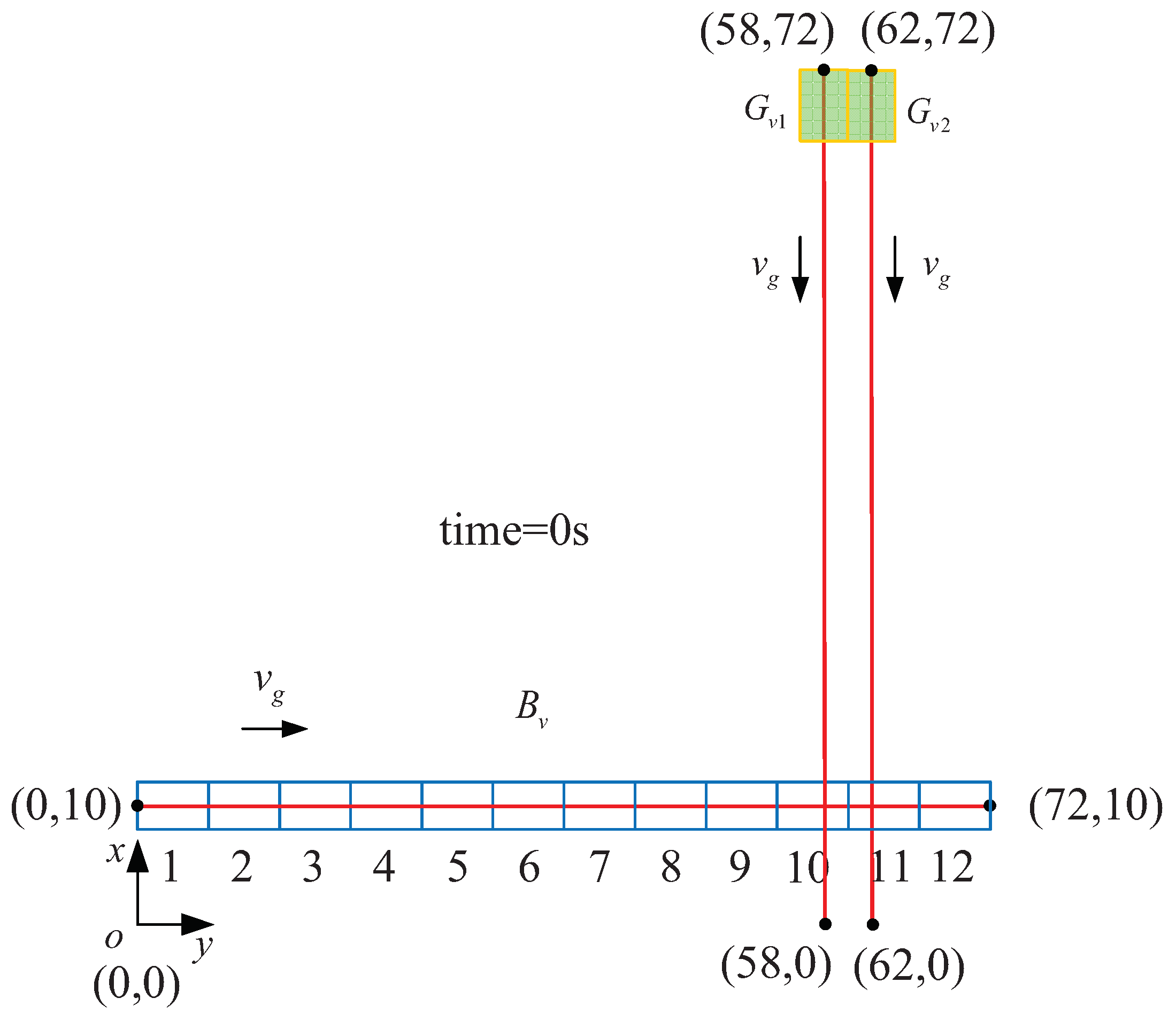
Consider two VGs (which are labeled as
and
, respectively) and a VB (labeled as
) as shown in
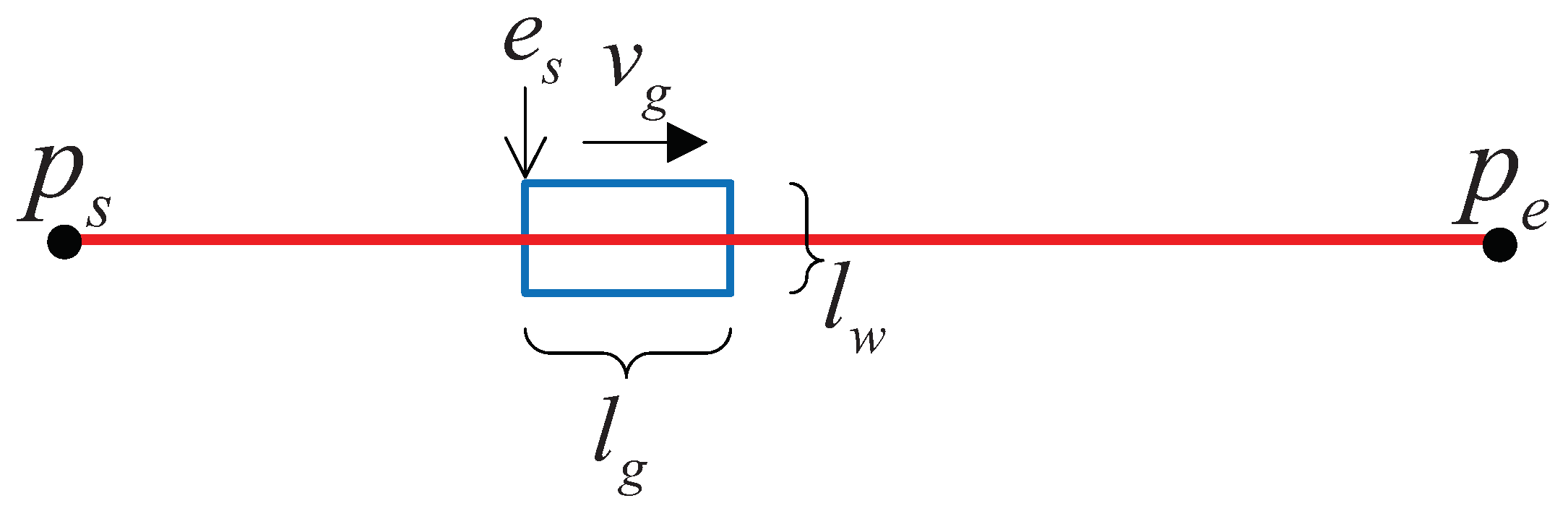
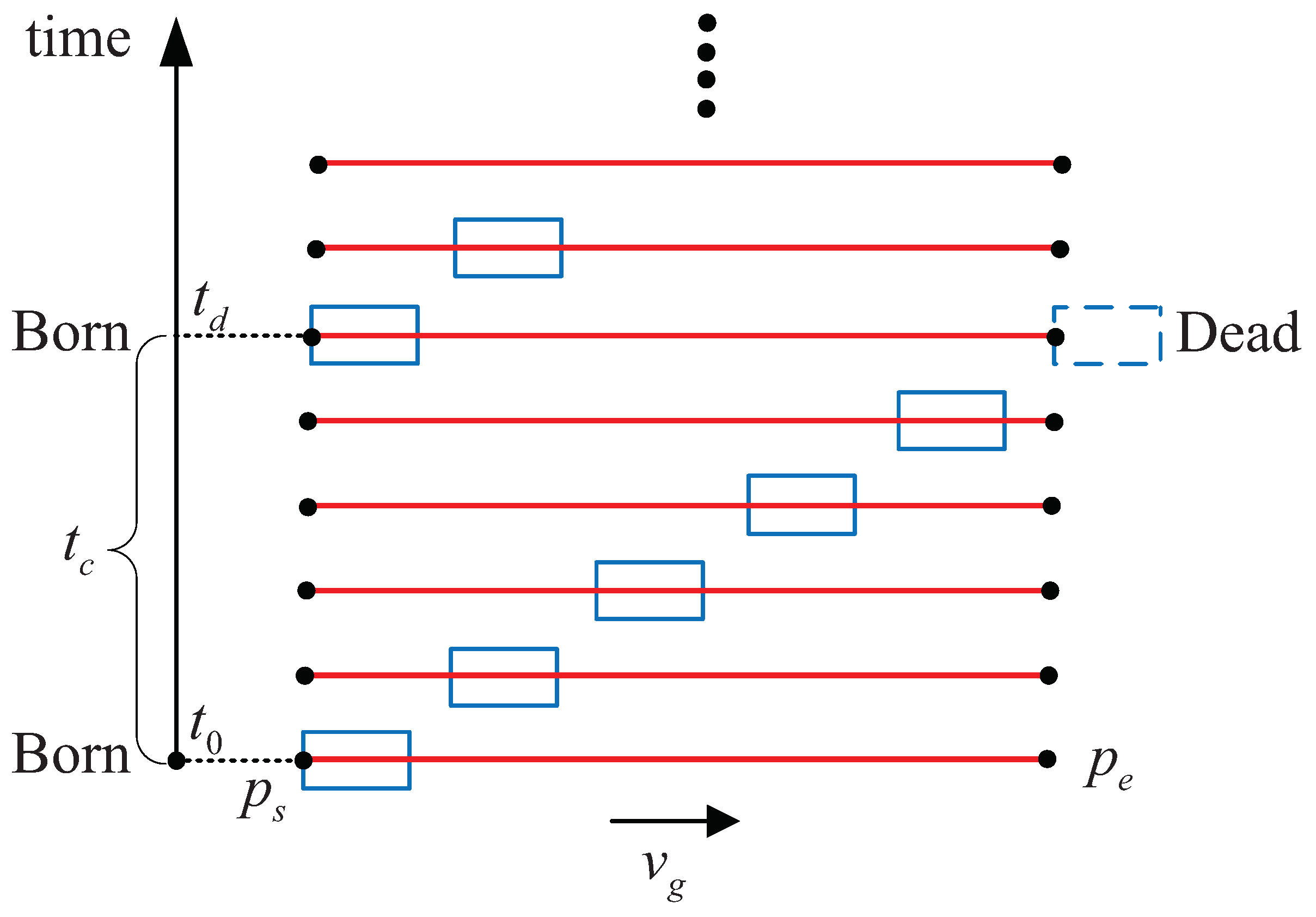
Figure 10. The VPs of these VGs and VB are plotted with solid red line in that figure. The coordinates of the start and end points of these VPs are shown in that figure as well. The unit of the coordinate is meter. The lengths of the three VPs are 72 m. There are twelve VGs on
, which are represented by
. All of these VGs are uniform.
= 6 m,
= 4 m,
= 2 m/s.
= 36 s.
| Algorithm 2 Calculation of the CVGR of A VG. |
Input: a set of VGs (S) and a VG ()
Output: the CVGR of - 1:
Initial an empty set - 2:
for in S do - 3:
call Algorithm 1. Collision checking of and - 4:
if collides with then - 5:
append to - 6:
end if - 7:
end for - 8:
return
|
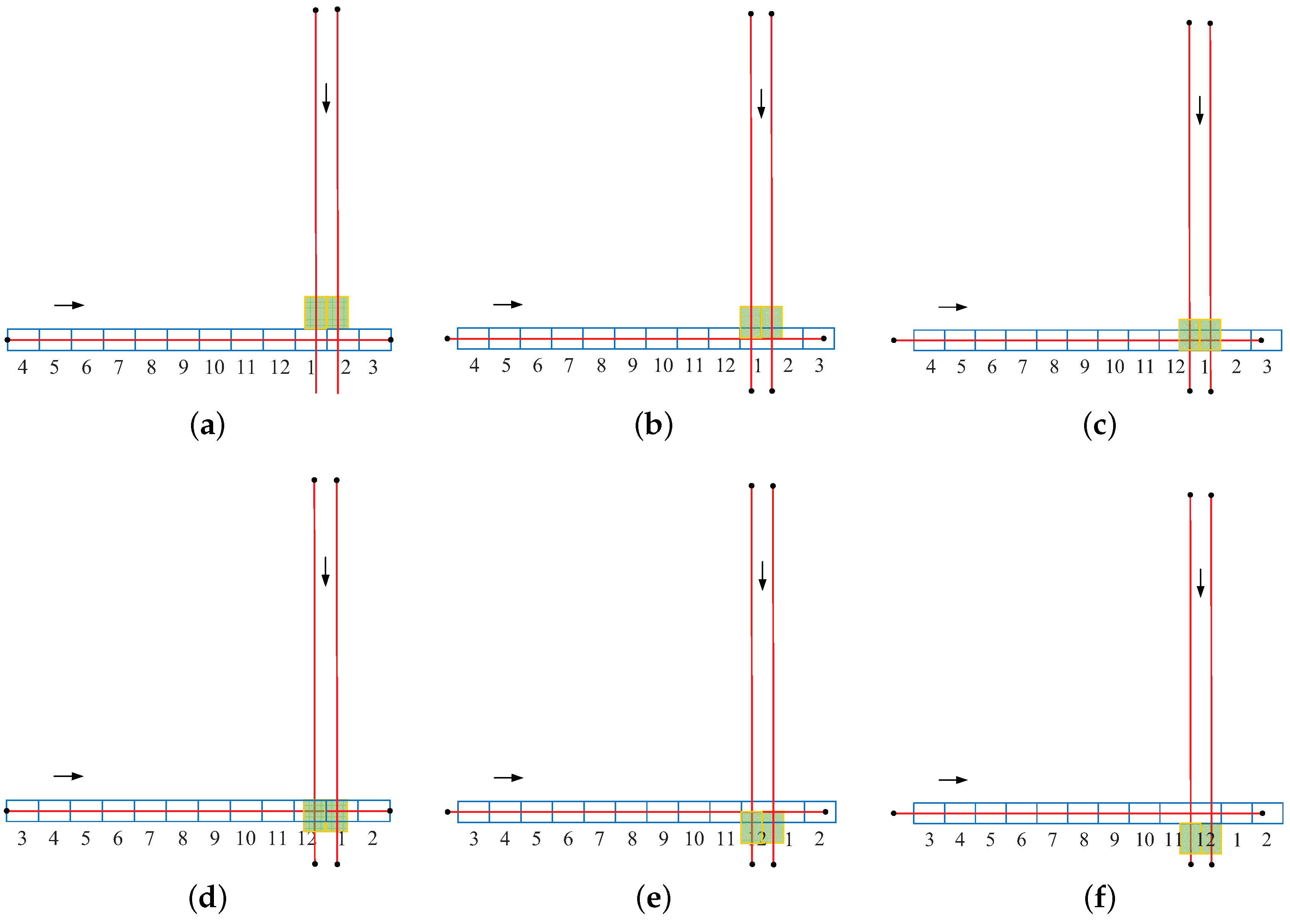
Several camera shots of
,
and
between 28 s and 33 s are plotted in
Figure 11. Using Algorithm 2, it can be found that
collides with
,
and
.
collides with
,
and
. The CVGR of
can be organized as {
,
,
}. The CVGR of
is {
,
,
}. Similarly, one can obtain that the CVGR of
is empty.
4.3. Collisions Checking of Virtual Belts
If the VGs in several VBs are uniform, the CVGR of each VG on these VBs can be obtained by Algorithm 2.
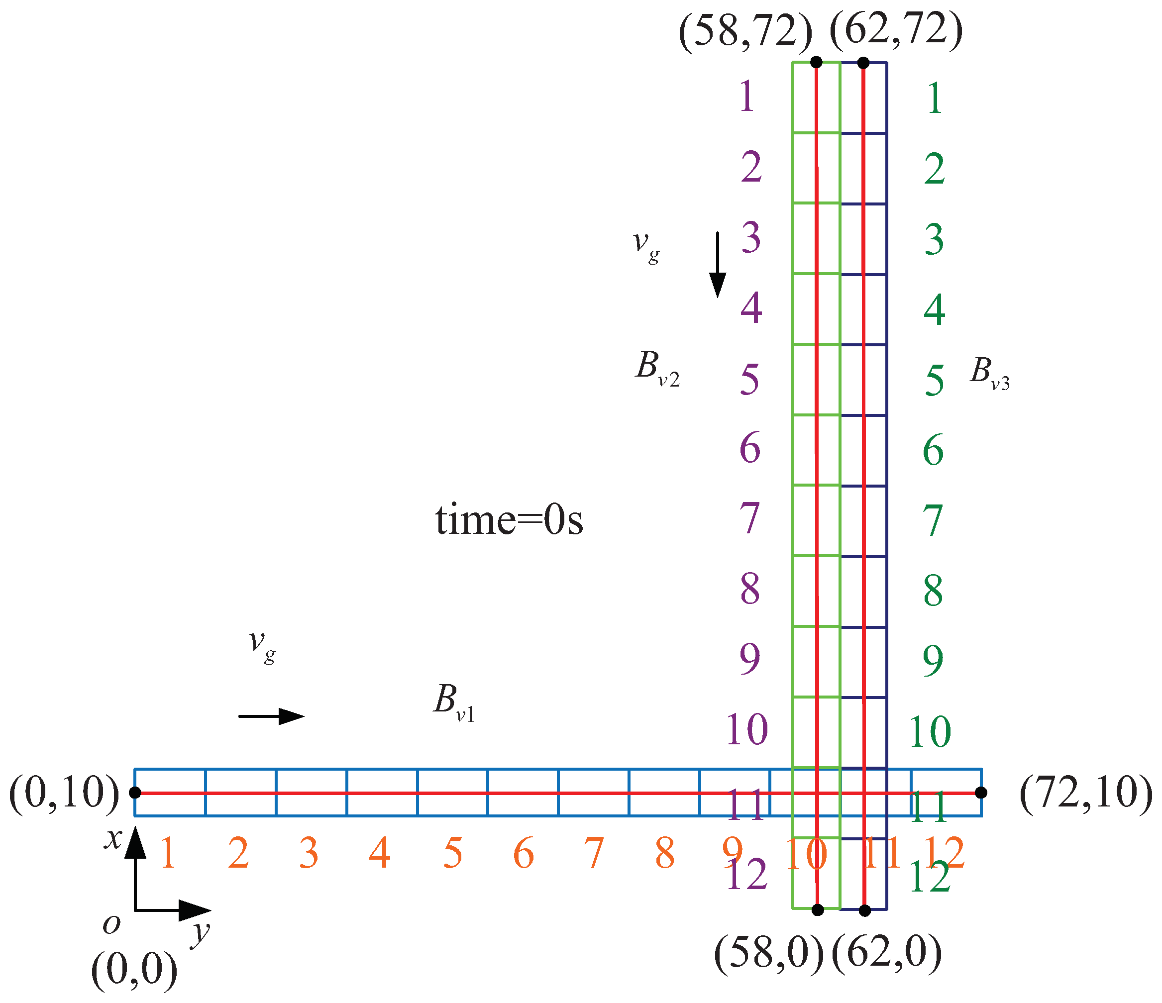
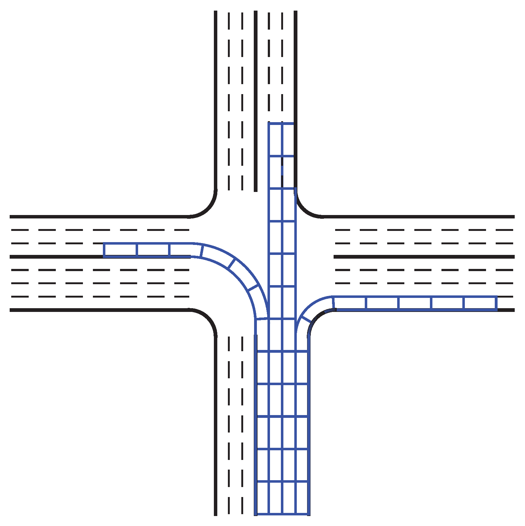
Consider three VBs as shown in
Figure 12. The coordinate unit is meter. These VBs are denoted by
. The VGs of
are represented by
, respectively.
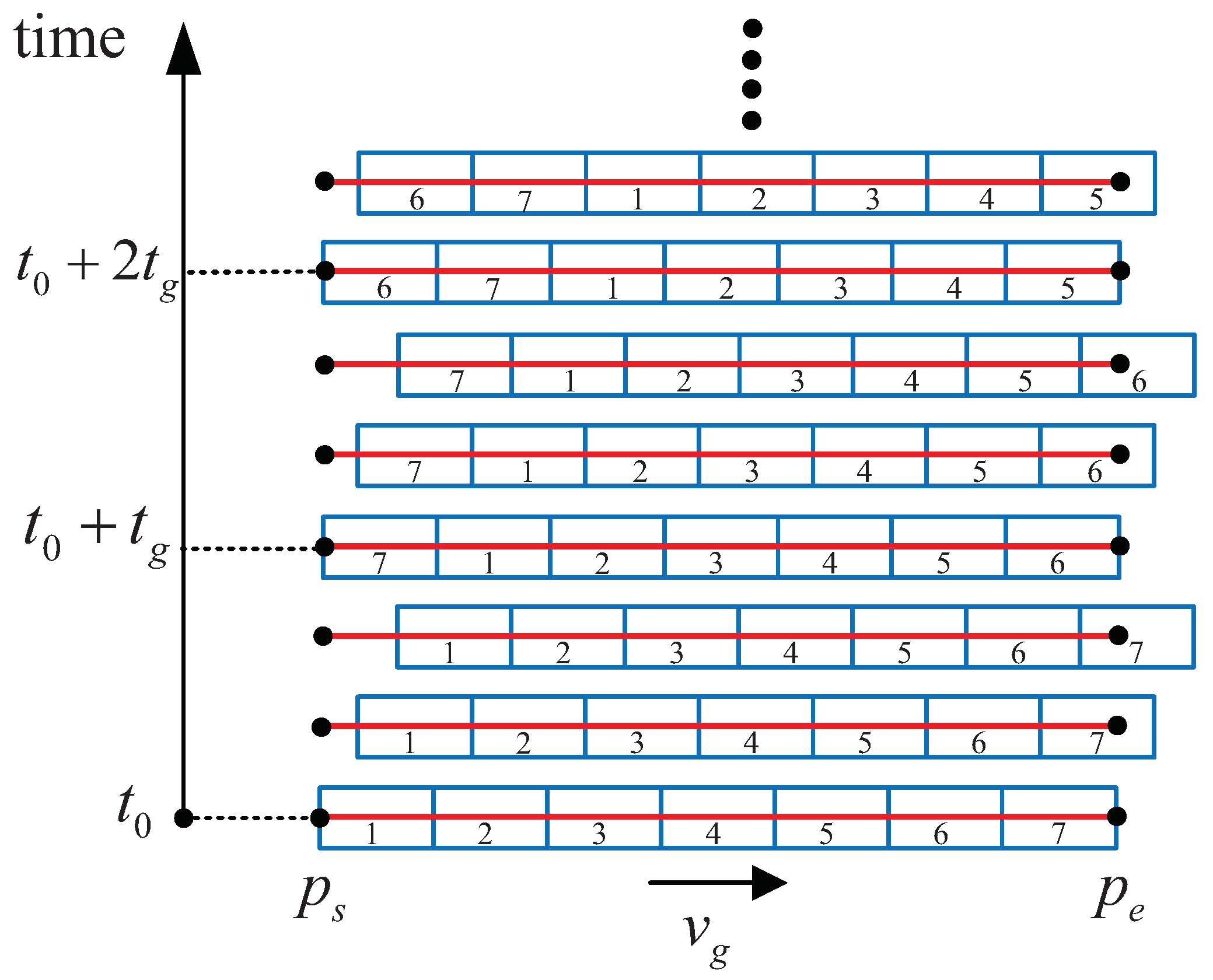
means the total count of the VGs in a VB. The VGs in these VBs are uniform. As demonstrated previous, the CVGR of
is
. Note that
will be the same position of
after the time of
. If
collides with
(which is a CVG of
) at the time of
t, then
will collide with
at the time of
. Thus, the CVGR of
, note that
, is
. The CVGR of
can be summarized as
. Similarly, the CVGRs of
and
are
and
, respectively.
5. Initial Idea of Virtual Belt Algorithm
In this section, the initial ideal of the proposed algorithm is discussed. Then an example to demonstrate the idea for intersection management is shown. At last several deficiencies of the initial ideal are discussed. This example demonstrates the basic principle of the proposed VB algorithm, which is made to facilitate the understanding of the core of the proposed VB algorithm.
5.1. Discussion of The Initial Idea
Consider that
and
(as shown in
Figure 9) are placed on an intersection with two through lanes. The start and end points of these VPs can be used to represent the departures and destinations of several approaching CAVs. The size of the VG is bigger than these CAVs. It is required that these CAVs should follow the trajectories of
and
to their destinations one by one without collision.
If a CAV is required to follow the trajectory of a VG to through the intersection, the CAV is called to be transferred by the VG and the VG is called assigned with the CAV as well. When a CAV arrives at the destination, it should move away from the intersection in constant speed to avoid affecting the “transfer service” of the intersection.
The VGs used for the transfer of CAVs should be selected carefully. An inappropriate choice may lead to collisions among CAVs. For instance, if the VGs demonstrated in
Figure 8 are used for CAV transfer, the approaching CAVs may collide with each other. If a VG and its CVGs are used for the transfer of CAVs simultaneously, collisions among these CAVs may occur. A natural idea is that when a VG is used to transfer a CAV, its CVGs should not be used. Thus, the collisions among CAVs can be avoided at the considered intersection.
The starting point of the initial idea is that several VBs are placed on the considered intersection. Each approaching CAV is assigned with a VG before the conflict points in the intersection. Thus, the approaching CAVs can follow the trajectories of the selected VGs and pass the intersection without collisions. Two requirements should be satisfied to ensure the safety of intersection management: First, the VGs which are assigned with CAVs should not collide with each other at the intersection. Second, the CAVs should be able to follow the planned trajectories with small tracking error.
5.2. Demonstration of the Initial Idea
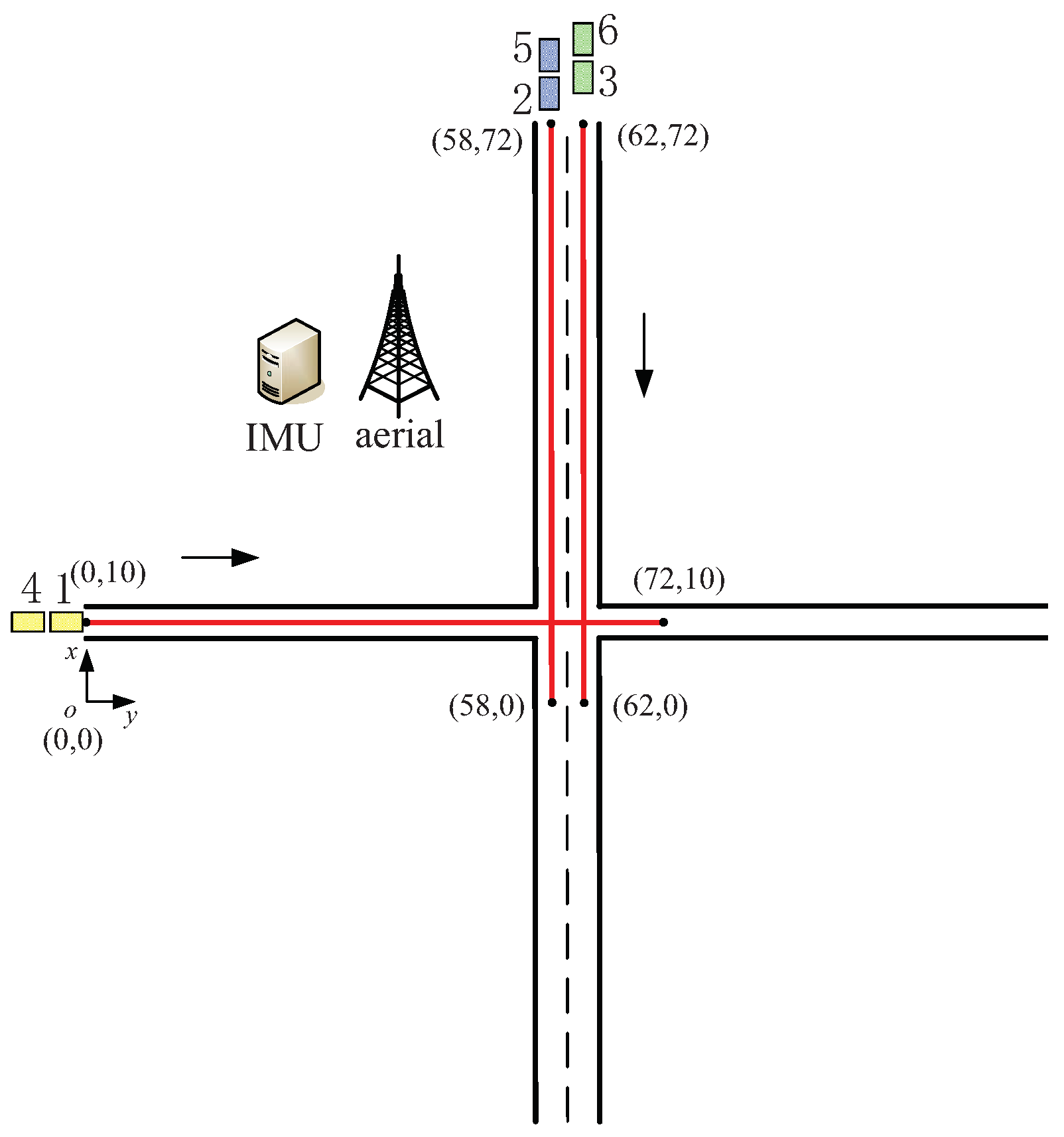
A simplified intersection with three through lanes is shown in
Figure 13. There are two approaching CAVs for each lane. According to the time of getting entry to the intersection, the orders of these CAVs are labeled from 1 to 6 as shown in this figure. The length and width of each lane are 120 m and 4 m, respectively. The length and width of these CAVs are 4 m and 2 m, respectively. It is preferred for these CAVs to pass the intersection with the speed of 2 m/s and least time delay. The collisions among these CAVs are prohibited. It can be found that there are potential collisions among these CAVs. Thus, these CAVs should be coordinated to pass the intersection by the IMU. The designed VPs based on the simplified intersection are shown in this figure as well. These VPs are the same as these shown in
Figure 12. Thus, the VBs in
Figure 12 are used to demonstrate the initial idea.
To show the initial ideal in a simple way, the dynamic limits of these CAVs are ignored. Thus, when a CAV is assigned to a VG, the CAV can reach the position of the VG with neglectable time. It is assumed that a CAV can keep a safe clearance with the front CAV in the same lane. These simplifications are made to show the initial idea of VB algorithm clearly. The VB algorithm considering the dynamic limits of CAVs will be designed next section.
Several definitions are made for VG to simplify the discussion:
A VG that approaches to the intersection is called a closing VG.
A VG that has been assigned with a CAV is called an occupied VG.
A VG without CAV is called a free VG. A occupied VG becomes free at the time of born.
A VG that may transfer a CAV cross the intersection with collision is called an unsafe VG.
Naturally, a collision avoidance policy can be proposed to prevent collisions among these CAVs: only the VGs before collision zone can be used for the transfer of CAVs. When a VG is occupied, the CVGs of the VG should be marked to avoid assignment of CAVs. Note that the mark should be cleared in certain conditions. Or a marked VG will not be utilized for CAVs forever, even all of its CVGs become free. To prevent such a condition, the mark will be cleared when the VG is dead. When a VG is born, it should be checked if there are potential conflict VGs. If a conflict VG is found, the VG should be marked to avoid usage. An unmarked VG before collision zones is called a candidate VG.
In order to avoid collision among CAVs, a policy is used to coordinate approaching CAVs: only a candidate VG can be used for the transfer of CAVs. The candidate VGs are ordered according to their distances to the intersection. The closer the distance, the higher order the VG. To transfer a CAV with the least time, it is preferred to assign a VG with the candidate VG with higher order.
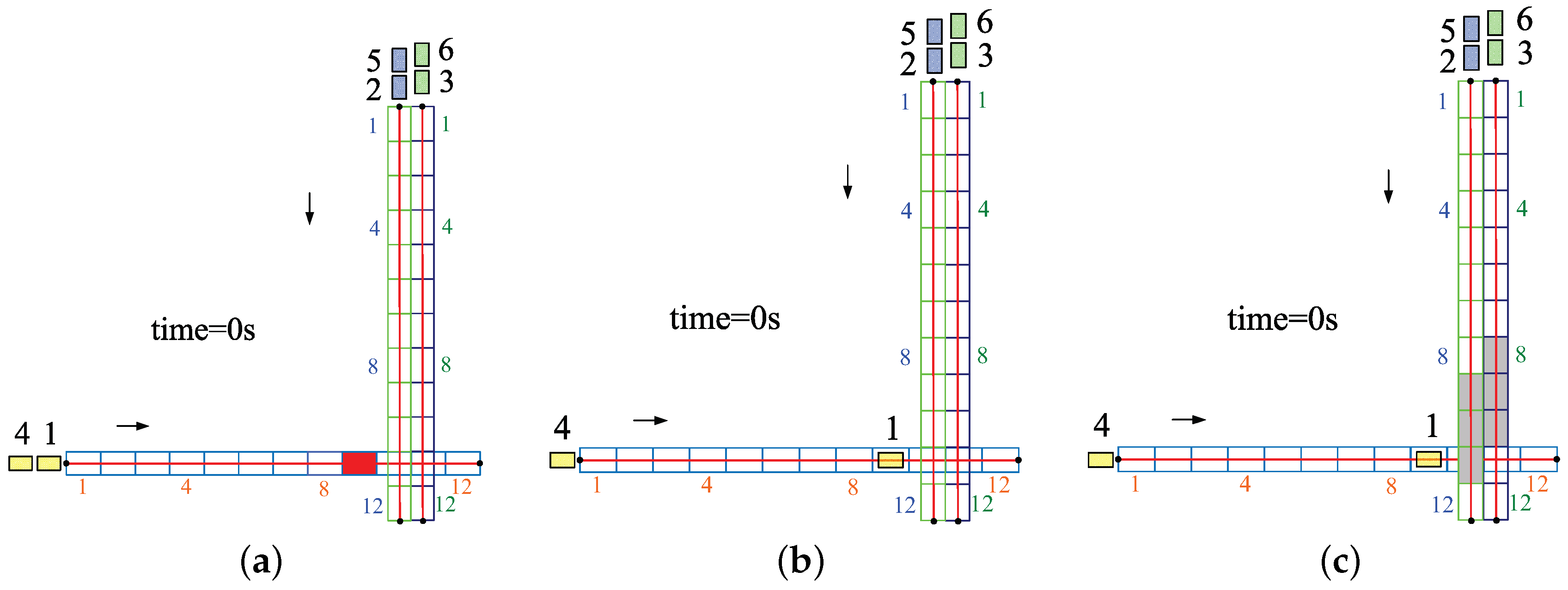
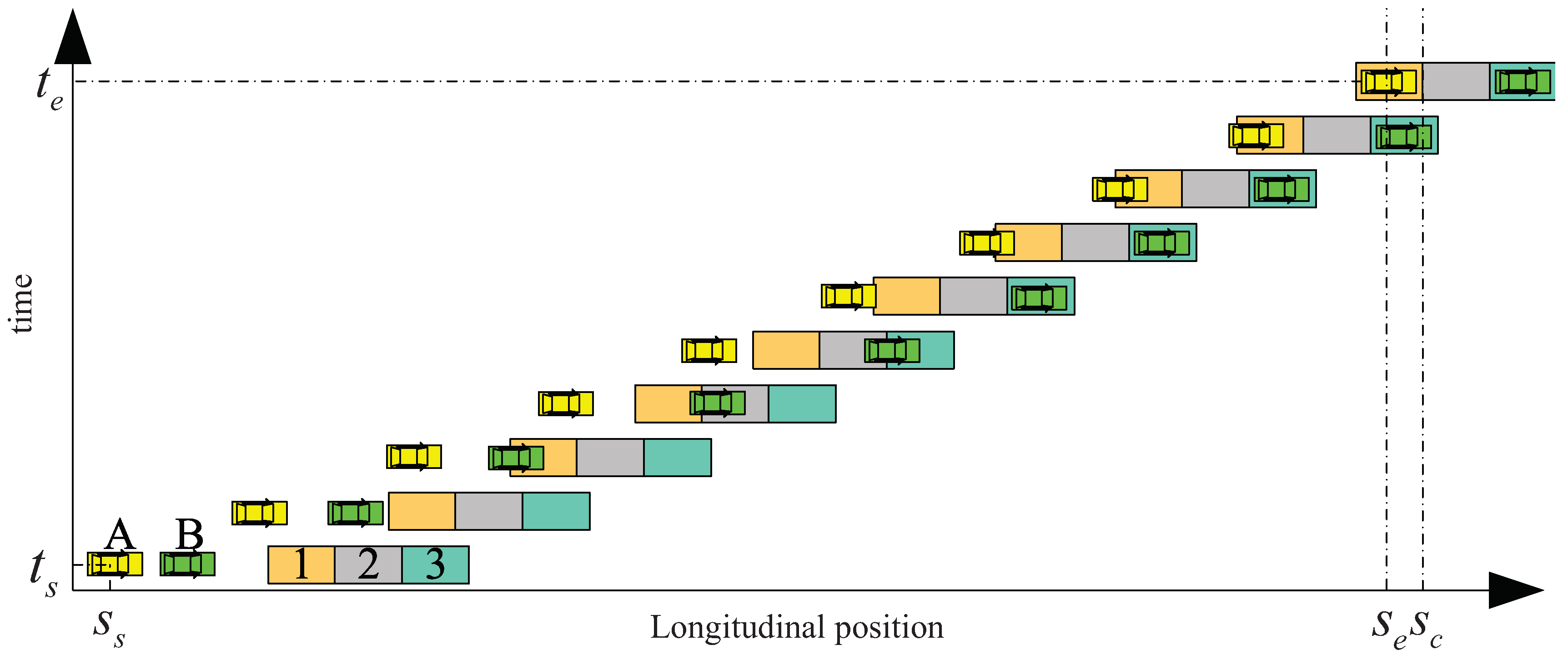
The steps to control CAVs to pass the intersection are shown below:
Step 1: At the time of 0 s, as shown in
Figure 14, find the VG (
) with the highest order in
for the first waiting CAV. Then, assign the first waiting CAV to
. Finally, mark the CVGs of
and fill them with gray.
When CAV 1 is assigned to , CAV 2 becomes the first waiting CAV. According to the assumption at the beginning of the section, the dynamic limits of CAVs are ignored in this section. It is assumed that a CAV can catch up with the assigned VG in no time.
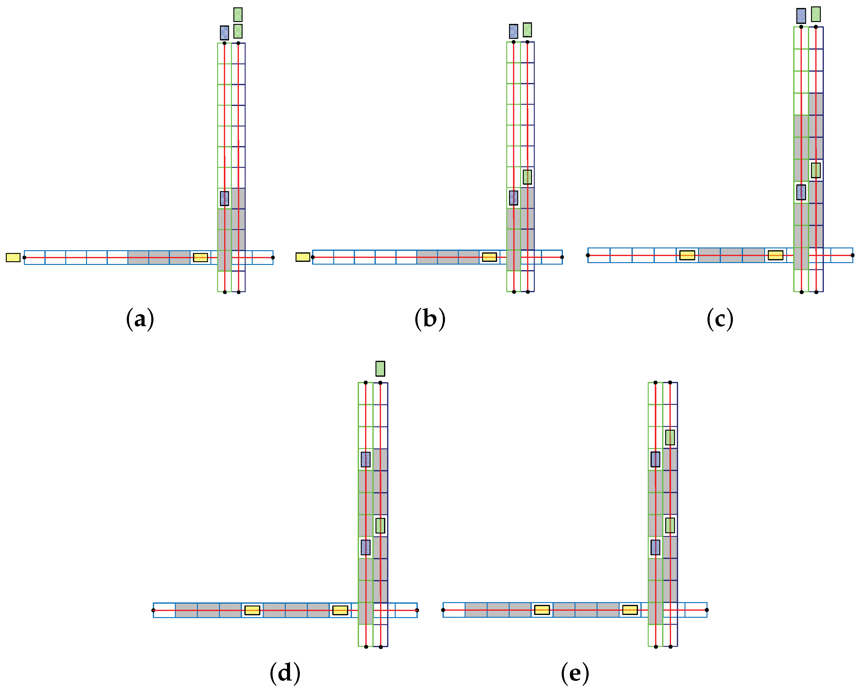
Similar to step 1, the other CAVs can be assigned to the optimal VGs with steps 2–6 as shown in
Figure 15.
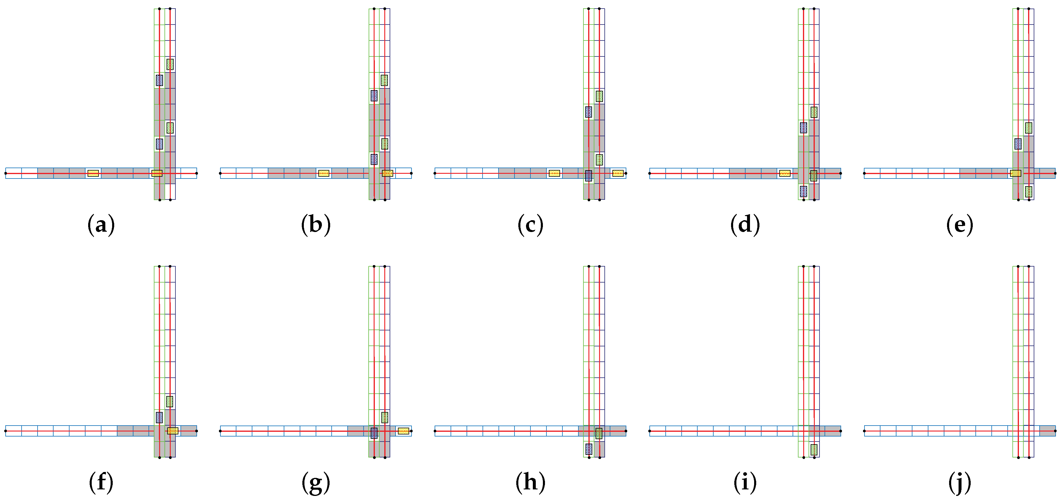
When all CAVs have been assigned with VGs, these CAVs can get through the intersection without collision as demonstrated in
Figure 16.
It can be seen from the above discussion that, the designed VBs can be used for the management of intersection. The trajectories of approaching CAVs can be selected among the trajectories of these VGs. Using simple VBs, the collision between the CAVs can be avoided. Provided longer VBs, more CAVs can be transferred in a time.
5.3. Deficiencies of The Initial Ideal
If all CAVs are in the corresponding assigned VGs, there will no collision occur among these CAVs as shown in
Figure 16. However, there are two deficiencies of the initial ideal, which make it difficult for practical application:
There are physical limits, such as maximum speed and acceleration, of CAVs. Thus, it is impractical for a CAV to catch up with the assigned VG in no time. As shown in
Figure 14, in fact CAV 1 has to spend some time to catch up with the assigned VG.
The performance of collision avoidance between the CAVs in the same lane cannot be guaranteed. As shown in
Figure 15, if CAVs 1 and 4 reach the assigned VGs simultaneously, then collisions between these CAVs may occur, which is not considered in the initial ideal.
These deficiencies can be resolved by planning a suitable trajectory considering actual physical constraints for each CAV. Following the planned trajectory, a CAV can catch up with the assigned VG and avoid collision within the physical limits. The method of trajectory planning will be discussed next section, which guarantees the feasibility of the proposed algorithm.
7. Numerical Simulation
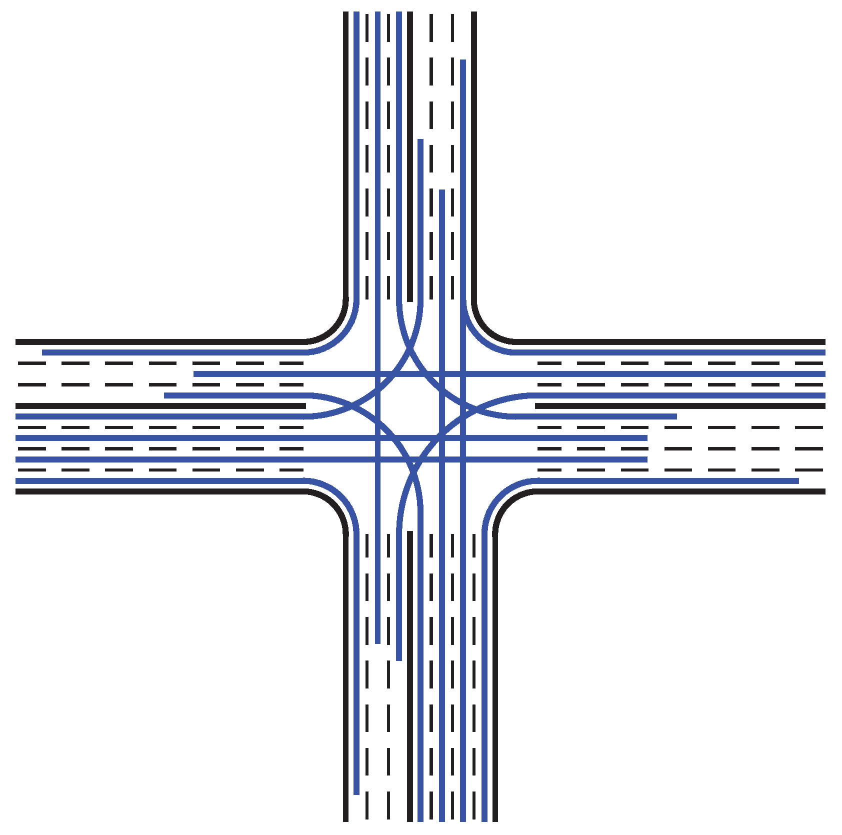
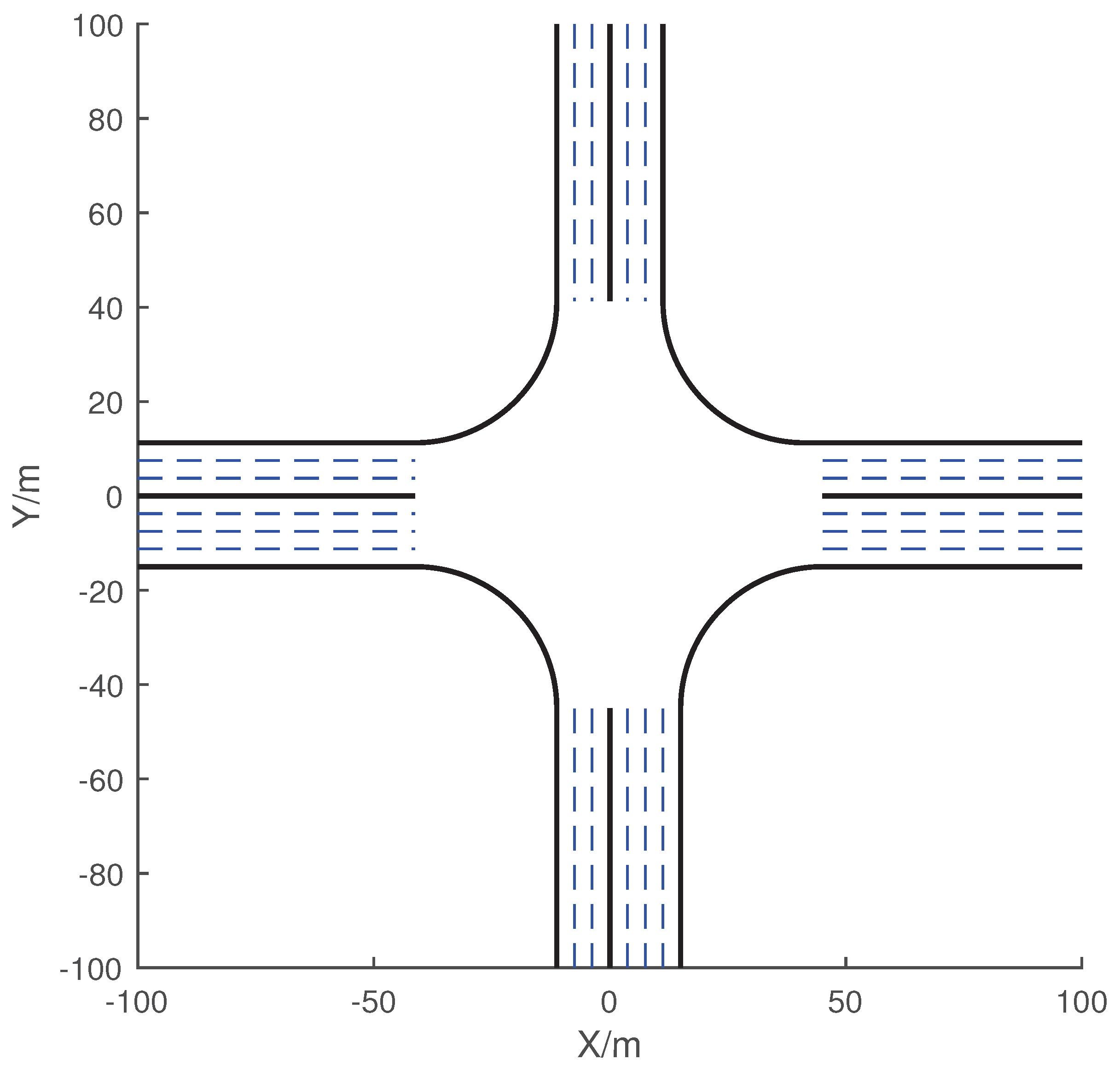
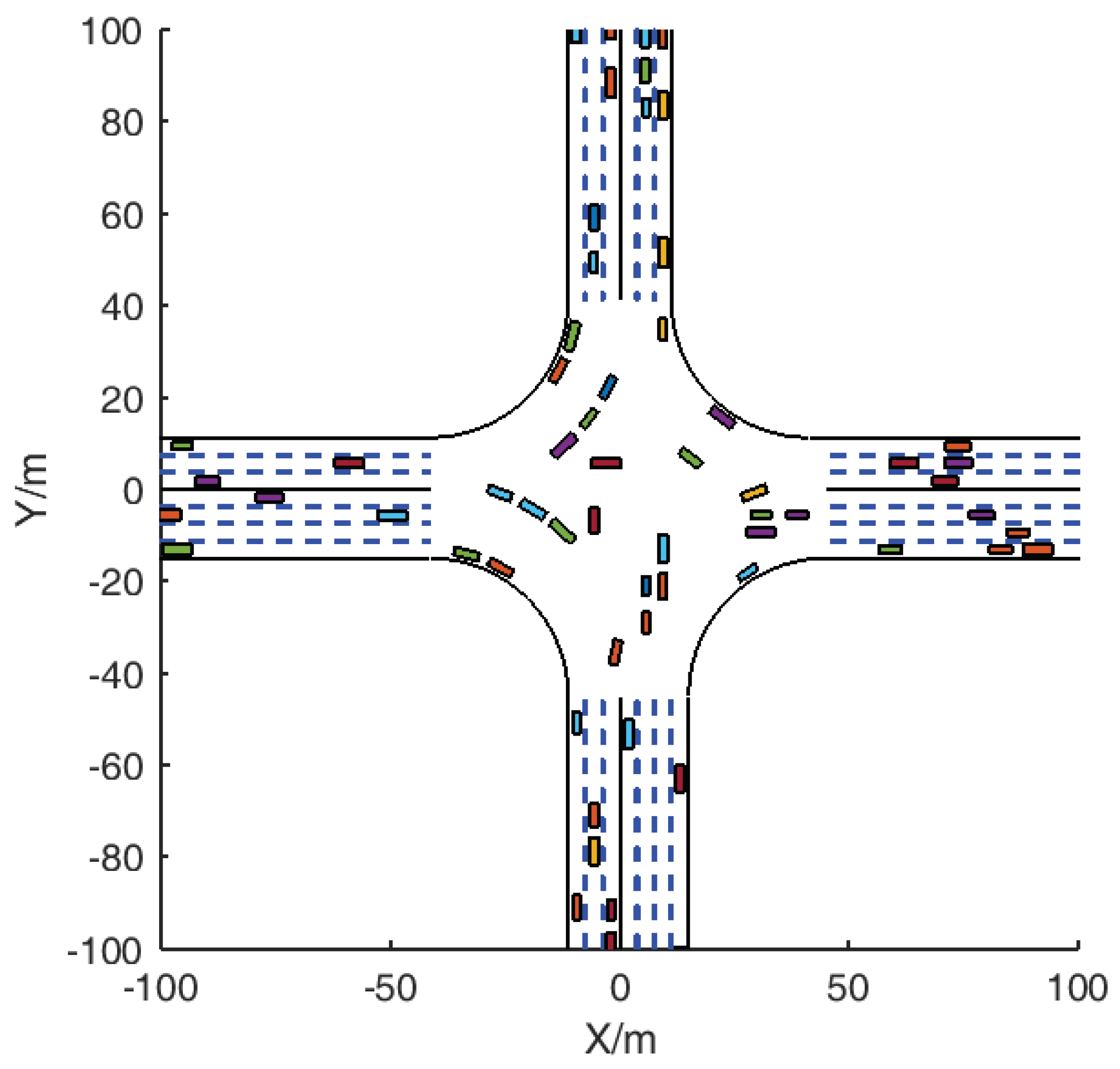
In this section, two simulations are conducted to verify the effectiveness of the proposed VB algorithm. The layout of the center of the considered intersection is shown in
Figure 20. In the first simulation, several scenarios with low traffic load are constructed to compare the performances of the VB algorithm, Multi-Agent (MA) algorithm [
1] and four-phase traffic lights with different green light time. In the second simulation, several scenarios with high traffic load are constructed to further compare the performances of these algorithms.
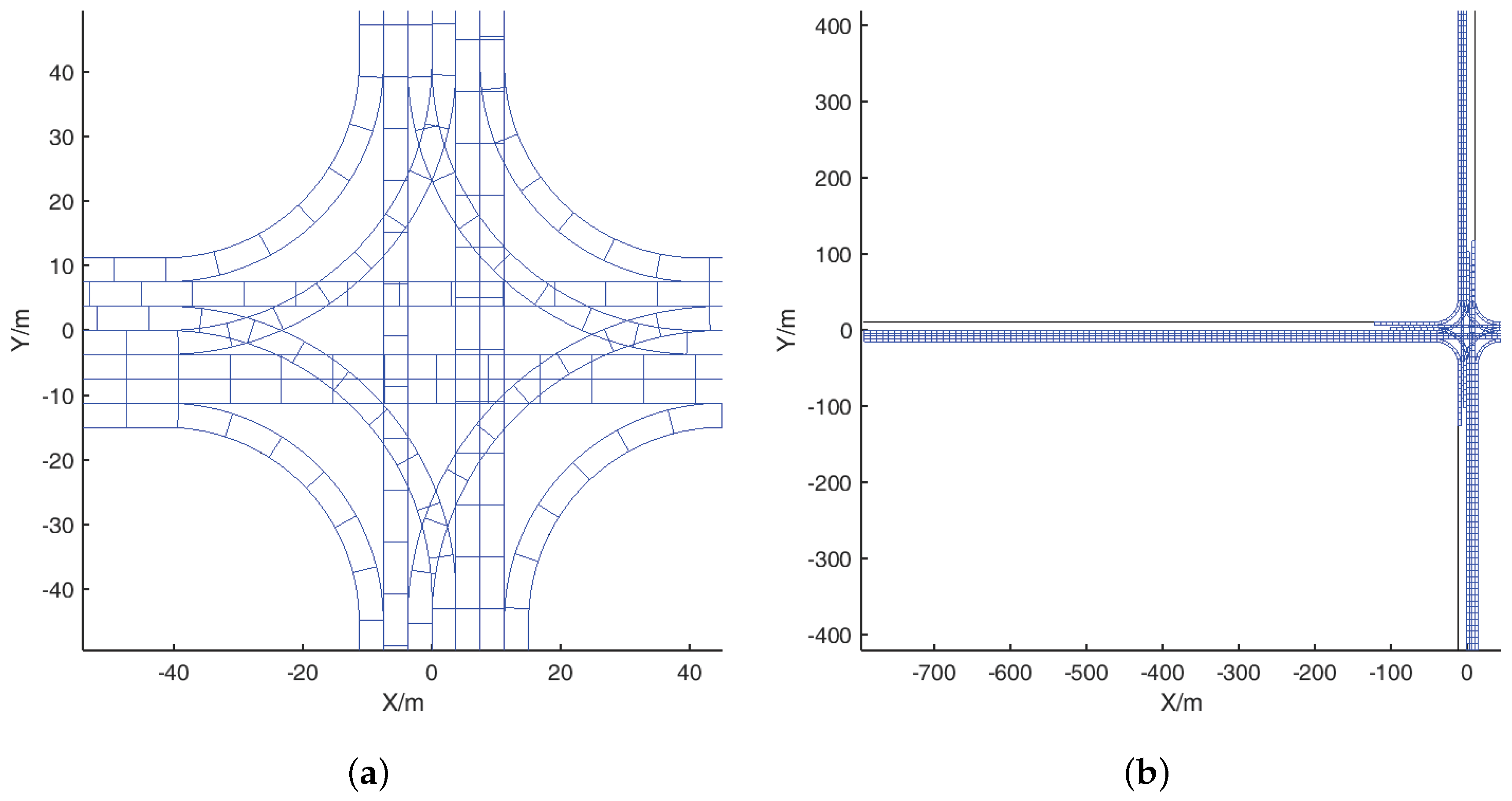
The VB and MA algorithms are performed using Matlab. Using the offline algorithm of the VB algorithm, the VBs designed at the intersection are illustrated in
Figure 21. The simulations of traffic lights are conducted using VISSIM. The parameters of the intersection and CAVs in these simulations are listed in
Table 1. A camera shot of the intersection controlled by the proposed VB algorithm is shown in
Figure 22. The proposed VB algorithm consists of an offline algorithm and an online algorithm. The offline algorithm is used to model the considered intersection using several VBs and calculate the collision among the VGs in these VBs. As the collision of each VG with all VGs in other VBs will be checked according to Algorithms 1 and 2, the complexity of the offline algorithm is
. Where
and
mean the count of VBs and the count of VGs in each VB, respectively. The online algorithm is used to calculate the trajectories of waiting vehicles in each circle one after another. The trajectory of a waiting vehicle can be obtained by successively checking the trajectories which are planned based on candidate VGs. As the candidate VGs of each vehicle is no more than
, the complexity of the online algorithm is
. Where
is the count of the waiting vehicles in each control circle. In the simulation, the computation time of the offline algorithm is about one hour. As the offline algorithm can be used before the real-time application of the VB algorithm, the time cost in the offline algorithm has no effect to the real-time performance of the VB algorithm. For the online algorithm, the time used to plan the trajectory of a waiting vehicle is less than 1 ms, which indicates that the proposed VB algorithm can be used for real-time application.
7.1. Simulation A
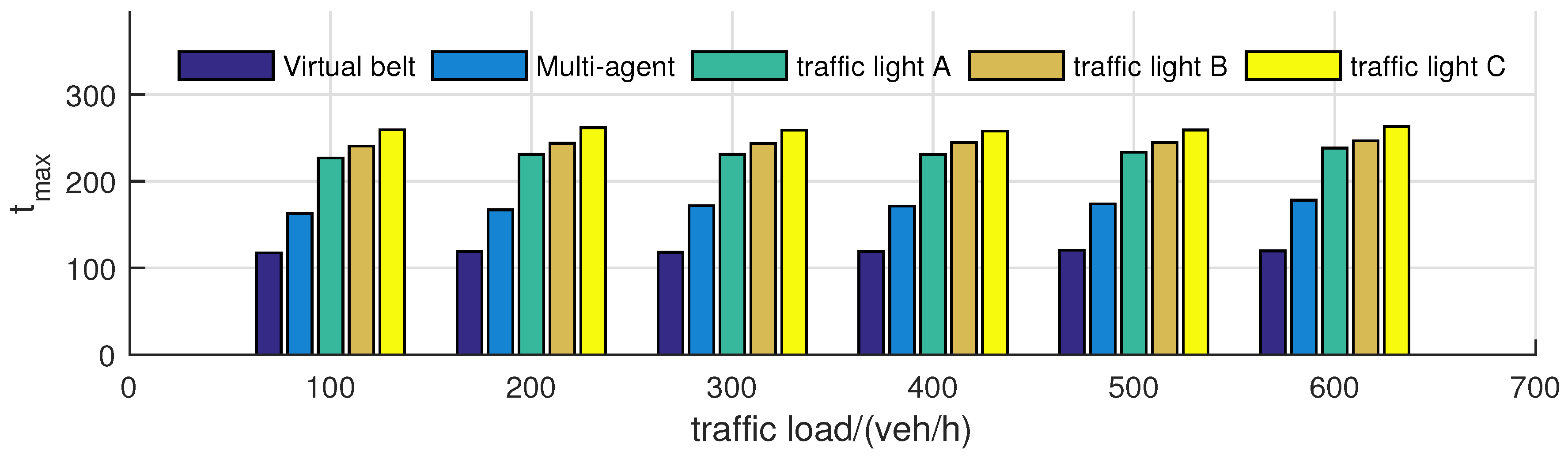
In this simulation, several scenarios are constructed to show the performance of the VB algorithm on low traffic load. The MA algorithm and traffic lights are used as comparison. The green times of these traffic lights are 17 s, 22 s and 27 s, which are denoted by TLA (traffic light A), TLB (traffic light B) and TLC (traffic light C), respectively. The mean traffic load of each road varies from 100 vehicle/h to 600 vehicle/h in the simulation.
Maximum travel time (
) is a commonly used index to compare the performances of different intersection management methods, which can be obtained by taking the maximum value of the travel times of all CAVs.
Figure 23 shows the maximum travel times of the intersections managed by VB, MA, TLA, TLB and TLC in 1800 s. The maximum travel times of the scenarios using VB algorithm are further plotted in
Figure 24.
Figure 23 suggests that with the growing of traffic load, the maximum travel times of the intersection controlled by these algorithms do not show notable increasement. This figure indicates that, on low traffic load, the change of traffic load has little effect on the performances of these algorithms. The maximum travel times of the traffic lights methods are about 250 s on different traffic loads. The maximum travel times of the MA algorithm are higher than 150 s but lower than 200 s, which are better than these of the traffic lights methods. As a comparison, the maximum travel times of the intersection controlled by the VB algorithm are lower than 150 s, which are much less than these of the MA algorithm. These comparisons indicate that, compared with traffic lights and MA algorithm, the VB algorithm can increase traffic efficiency and save travel time for CAVs on low traffic load. The main reason is that the CAVs can be coordinated by the VB algorithm without waiting for the green light. Several candidate trajectories can be selected to find the optimal one for each CAV. Thus, they can pass the intersection with constant desired speed and little delay. For the traffic lights methods, the CAVs have to wait for green lights, which is low efficient and time consuming on low traffic load. For the MA algorithm, on low traffic load, there are a few conflicts among the trajectories of approaching CAVs. Most of these CAVs can pass the intersection without delay. While, when there is a conflict between the trajectories of two CAVs, one of these CAVs has to slow down and wait for permission next control circle. Thus, the MA algorithm shows better performance than the traffic light but worse than the VB algorithm on low traffic load.
7.2. Simulation B
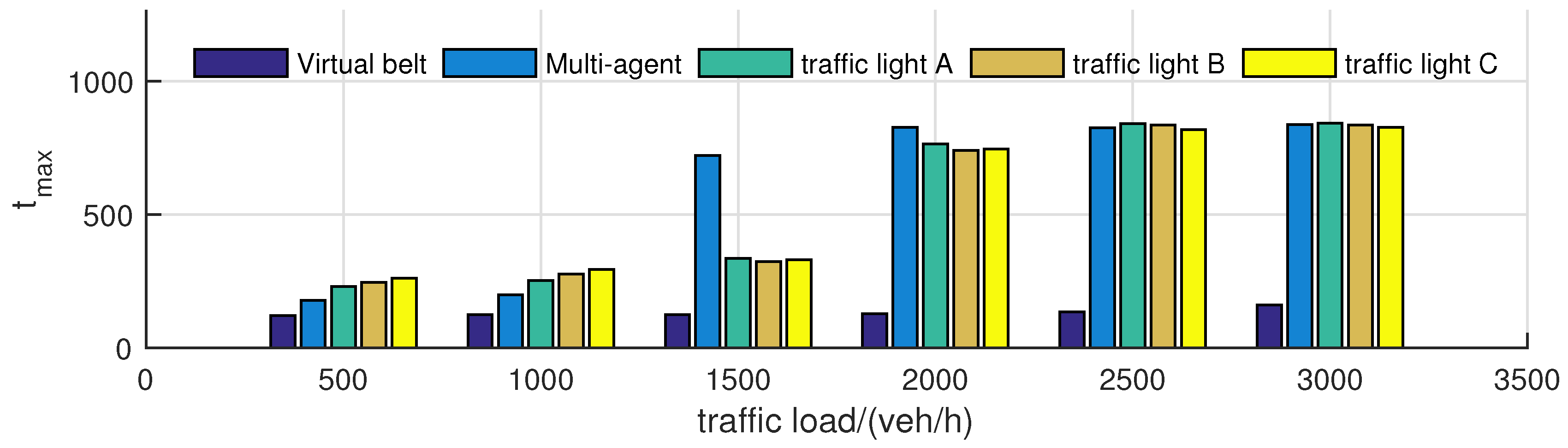
In this simulation, several scenarios are constructed to show the performance of the VB algorithm on high traffic load. The MA algorithm and traffic lights are used as comparison. The mean traffic load of each road varies from 500 vehicle/h to 3000 vehicle/h in the simulation.
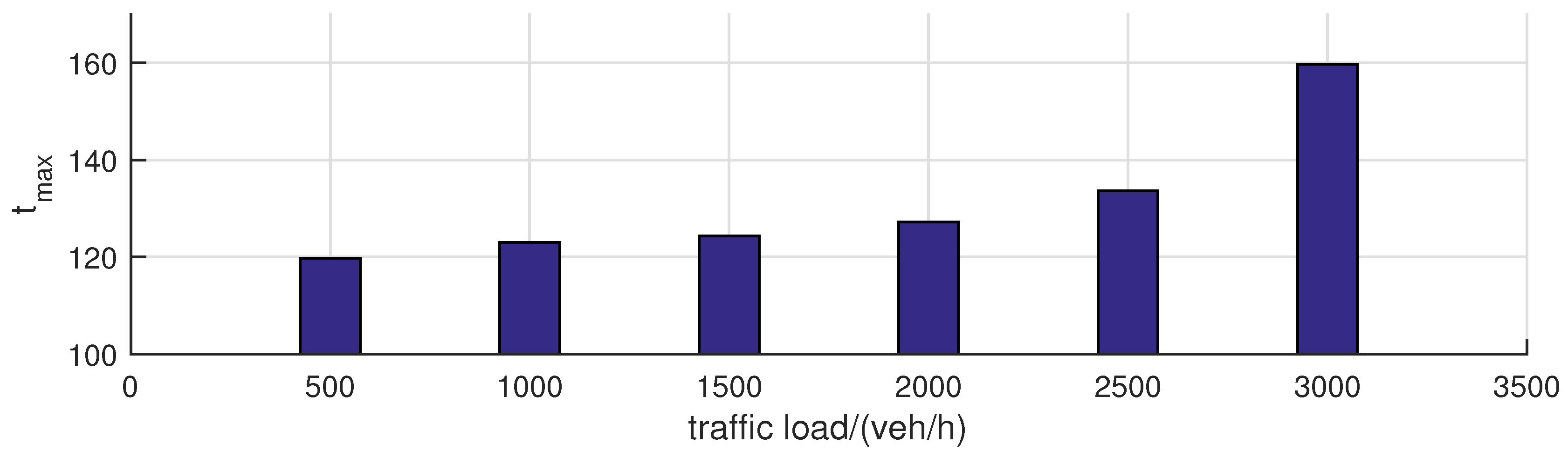
Figure 25 shows the maximum travel times of the intersections managed by VB, MA, TLA, TLB and TLC in 1800 s. The maximum travel times of the scenarios using VB algorithm are further plotted in
Figure 26.
Figure 25 suggests that with the growing of traffic load, the maximum travel times of the intersection controlled by TLA, TLB and TLC increase remarkably. The maximum travel times exceed 500 s on the traffic load of 2000 vehicle/h. The MA algorithm shows better than the TL algorithm just on the traffic load of 500 vehicle/h and 1000 vehicle/h. The maximum travel time shows a notable increase on the traffic load of 1500 vehicle/h, which is worse than the traffic lights methods. This is because on high traffic load, there are more conflicts among the trajectories of approaching CAVs. Most of these CAVs with conflicts will stop before the collision zone, which leads to much loss of time. As a comparison, the maximum travel time of the intersection controlled by the VB algorithm shows less increasement than other algorithms, which is below 170 s as indicated in
Figure 25 and
Figure 26. The main reason is that, on high traffic load, the CAVs can be coordinated by the VB algorithm using trajectory planning to avoid collision. And less CAVs need to wait before the intersection. Thus, the traffic efficiency can be improved than the compared algorithms. These comparisons indicate that the VB algorithm can increase traffic efficiency and save travel time greatly for CAVs on high traffic load.
8. Conclusions
This study proposes VB algorithm for intersection management to improve traffic efficiency of intersections. The proposed VB algorithm not only can be used for commonly discussed intersection, but also provides a framework to the investigation of general intersection management. As the VBs can be constructed based on the vehicle paths, the offline algorithm can also be applied for roundabout and other types of intersections without modification. Moreover, as indicated in the considered intersection, the overlap among VBs is also acceptable for the VB algorithm. Thus, the offline algorithm provides a flexible way to model an intersection. Because the calculation of the offline algorithm can be done before real-time application, the complexity of the intersection will not affect the real-time performance of the VB algorithm. When an intersection is modeled as several VBs, the online algorithm can be utilized to plan the trajectories of waiting vehicle to pass the intersection. The core of the online algorithm is that, based on the constructed VBs, several candidate trajectories can be selected for each approaching CAV. Thus, there are more opportunities can be provided by the VB algorithm for an approaching CAV through the intersection. Since the constraints of the speed and acceleration of CAVs are considered, the online algorithm can be used for different kinds of vehicles on road, which guarantees the flexible of the VB algorithm to common vehicles. In the simulation, instead of a homogeneous intersection with a symmetrical structure, an inhomogeneous intersection with a general structure is considered to represent a general case. The counts of VBs in different roads are not the same and there are overlaps among these VBs. Moreover, the considered CAVs are of different dynamic performances, such as maximum speed and maximum acceleration. The successful application of the proposed VB algorithm indicates that this algorithm is effective to manage such a general intersection.
There are three research directions for the future investigation: The first one is to apply the VB algorithm to other types of intersection, such as roundabout and 3-way intersection. The second one is to extend the VB algorithm to the management of multi-intersection. The third one is to investigate the VB algorithm with the fuel economy performance.


