Article

Analysis of Some Empirical Equations for Modeling Sound Absorption of Porous Absorbers

by
Valentín Gómez Escobar
* and
Celia Moreno González
Departamento de Física Aplicada, Escuela Politécnica, Institute for Sustainable Regional Development (INTERRA), Universidad de Extremadura, Avda. de la Universidad s/n, 10003 Cáceres, Spain
*
Author to whom correspondence should be addressed.
Materials 2026, 19(14), 3128; https://doi.org/10.3390/ma19143128
Submission received: 9 June 2026 / Revised: 14 July 2026 / Accepted: 15 July 2026 / Published: 21 July 2026
(This article belongs to the Section Advanced Materials Characterization)

Abstract

The empirical Delany–Bazley model and several of its subsequent modifications were evaluated to determine their ability to predict the sound absorption coefficient spectra of porous materials. The study considered three porous materials (foam, mineral wool and samples made from recycled cigarette butt) with different thicknesses. Model performance was assessed by comparing theoretical predictions with impedance tube measurements using the root mean square error (RMSE). Although some models yielded lower prediction errors for specific materials and thicknesses, the results showed that sample thickness—and the associated changes in the shape of the sound absorption spectrum—have a greater influence on model performance than the material itself. No single empirical model consistently provided the best agreement over the entire thickness range. These findings suggest that the applicability of Delany–Bazley-type empirical models appears to be more closely related to the shape of the sound absorption spectrum than to the material for which they were originally developed. These findings provide practical guidance for selecting suitable models for both conventional and recycled porous sound absorbers.

1. Introduction

Sound-absorbing materials play a key role in the acoustic treatment of rooms and are also widely used in multilayer sound insulation systems.
Porous materials constitute one of the most important classes of sound absorbers. They are characterized by interconnected pores or cavities through which sound waves propagate while losing part of their energy due to thermal and viscous effects. According to their microscopic structure, porous materials can be classified as granular, fibrous, or cellular [1].
Several models have been proposed to predict the acoustic behavior of porous materials. They can be classified as theoretical, microstructural, and phenomenological. A review of some of them can be found elsewhere [2,3]. Apart from their theoretical formulation, the main difference between these models lies in the number of parameters required for the calculation. Because some of the parameters needed by the theoretical models (e.g., porosity, tortuosity, thermal characteristic length, and airflow resistivity) are difficult to determine experimentally, one of the most widely used models is the empirical model proposed by Delany and Bazley [4], which requires only a single parameter: the airflow resistivity of the sample.
Several authors have applied the Delany–Bazley model to compare theoretical predictions with experimental results [5,6,7,8,9,10]. Other authors have proposed modifications to the coefficients of the Delany–Bazley model to adapt it to materials different from the commercial fibrous absorbers (fiberglass and mineral wool) originally considered by Delany and Bazley. Thus, Dunn and Davern [11], Wu [12], and Miki [13] proposed modified versions of the Delany–Bazley model for open-pore polyurethane foams and plastic open-cell foams, and for double-layer porous materials, respectively. Later, Garai and Pompoli [14], Ramis et al. [15], Arenas et al. [16], and Rey et al. [17] proposed further modifications to the original coefficients for polyester-, kenaf-, cellulose-, and sheep wool-based materials, respectively. Recently, Dunne [18] proposed an ‘optimized Delany-Bazley model’ for both synthetic and natural fiber materials.
More recently, other authors have determined optimized coefficients for the Delany-Bazley equation for individual samples [19,20].
In recent years, our research group has investigated the development of a sound-absorbing material produced by recycling used cigarette butts [21,22]. Accordingly, the first objective of the present work is to evaluate the suitability of the original Delany–Bazley equation and several of its modified versions for predicting the acoustic performance of sound-absorbing samples manufactured from recycled cigarette butts.
However, the shape of the sound absorption spectrum is strongly influenced by sample thickness [23,24,25,26]. This raises the question of whether a single empirical model is sufficient to fit the experimental data or whether the predictive capability of these empirical models depends primarily on the type of porous material or on the shape of the sound absorption spectrum itself. Therefore, the second objective of this work is to evaluate the suitability of these equations for samples with different thicknesses and, consequently, different sound absorption spectra.
Finally, to assess the generality of the proposed approach, two additional porous materials, namely a cellular foam and commercial mineral wool, were also investigated.

2. Materials and Methods

2.1. Instrumentation for the Determination of Acoustic Properties

When a sound wave impinges on a material, part of the incident wave is reflected (Er), and the remainder of the wave is either dissipated within the material or transmitted through it. Accordingly, the sound absorption coefficient (α) is defined as the ratio of the non-reflected sound wave energy (EiEr) and the incident energy (Ei). Therefore:
α =   E i E r E i
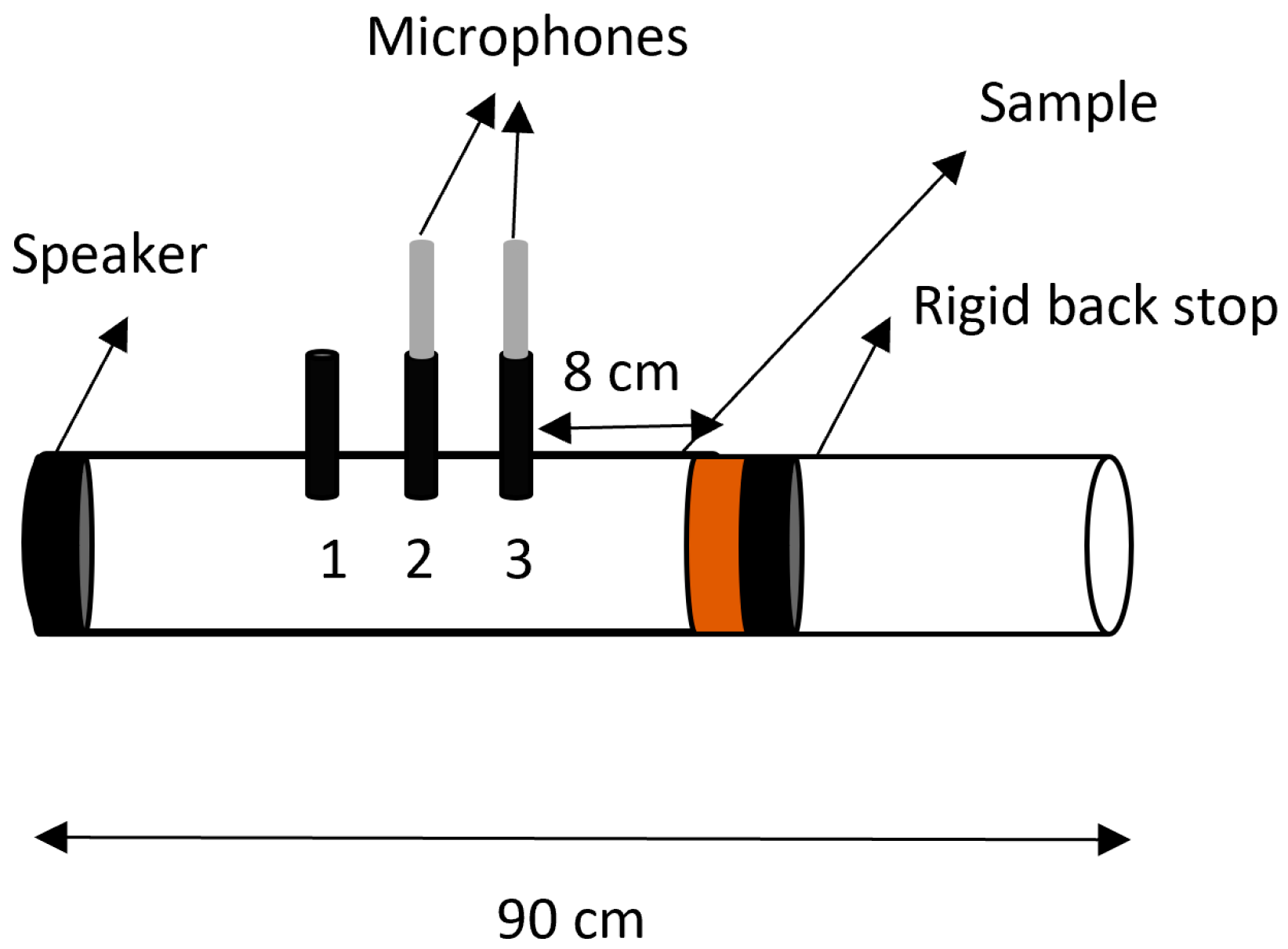
There are different methods for the determination of the sound absorption coefficient. In this work, the sound absorption coefficient of the samples was determined using an impedance tube, following the two-microphone transfer-function method described in the ISO 10534–2 standard [27].
The measurements were performed using a Brüel & Kjær Impedance Tube Kit (Type 4206, Copenhagen, Denmark), equipped with two one-quarter-inch condenser microphones (Type 4187). Signal acquisition and analysis were carried out using a portable Brüel & Kjær PULSE System (Type 3560-C) with four input channels. Sample holders with diameters of 29 and 100 mm were used, providing valid frequency ranges of 500–6400 Hz and 50–1600 Hz, respectively.
The experimental configuration used for the sound absorption measurements is shown in Figure 1.
Airflow resistivity (σ) is a fundamental property of porous materials and quantifies the resistance offered by the pore structure to airflow. It is expressed in Pa·s/m2 and is related to the airflow resistance (R) (defined as the ratio of the pressure drop across the sample to the airflow velocity through it), according to:
σ =   R · A d
where A is the cross-sectional area of the sample and d is the sample thickness.
The airflow resistivity of the samples analyzed in this work was determined using the Ingard and Dear method [28]. The experimental sample configuration inside the impedance tube was the same as described in previous work [29]. The airflow resistivity was determined from the sound pressure levels measured by the two microphones. Following the procedure proposed by Juliá Sanchís [30], the difference between the sound pressure levels at the first minimum of the Lp1 − Lp2 spectrum was used to calculate the normalized airflow resistance and, subsequently, the airflow resistivity.

2.2. Preparation of Samples

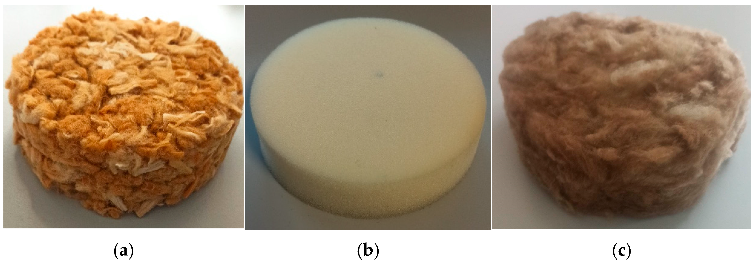
Three different types of materials were considered for the present study: one cellular (foam samples) and two fibrous (commercial mineral wool and samples prepared by disaggregating used cigarette butts). The commercial mineral wool samples were cut directly from commercial panels, whereas the foam samples were supplied with the impedance tube kit as reference materials. The used cigarette butts for the third group of samples were conditioned as described in previous work [29], without chemical cleaning, and subsequently disaggregated using a grinder. Representative photographs of the prepared samples are shown in Figure 2.
Samples were prepared in two sizes, both circular, with diameters of 29 and 100 mm according to the two diameter sizes of the used impedance tube. As mentioned above, previous studies show that the sound absorption coefficient spectrum was influenced by the thickness of the sample. Thus, for each type of sample, several samples of different thicknesses were made. No compression was applied during sample preparation; therefore, differences in density among samples of the same material were minimal. The bulk density of each sample was determined by weighing the samples and calculating their bulk density. The measured bulk density ranged from 63 to 71 kg/m3 for butt-derived samples, from 25.9 to 27.1 kg/m3 for foam samples, and from 36 to 41 kg/m3 for mineral wool samples. The number of samples prepared and their thickness ranges are summarized in Table 1.
The airflow resistivity estimated using the Ingard and Dear method exhibited a marked dependence on sample thickness. Values ranging from 3 to 15 kPa·s/m2 were obtained for the foam samples, from 1 to 12 kPa·s/m2 for the mineral wool samples, and from 1 to 7 kPa·s/m2 for the butts-derived samples. This variation in thickness was consistent with the changes observed in the sound absorption spectra, which will be described below.

2.3. Theoretical Equations

The Delany and Bazley model describes the acoustic behavior of porous materials in terms of two complex variables: the characteristic impedance (Z0) and the propagation coefficient (γ) according to the following general equations:
Z 0 =   ρ 0 · c 0 1 + C 1 ρ 0 f σ C 2 j · C 3 ρ 0 f σ C 4
γ = ω c 0 C 5 ρ 0 f σ C 6 + j   1 + C 7 ρ 0 f σ C 8
where the coefficients C1 to C8 proposed by Delany and Bazley are those indicated in Table 2 (Model M1).
Although some authors prefer to use the complex wave number (kc) (radians per meter or m−1), instead of the propagation coefficient (γ) [2,6,31]:
k c =   ω c 0 1 + C 7 ρ 0 f σ C 8 j   C 5 ρ 0 f σ C 6  
which is equivalent to Equation (4) considering that kc = j·γ.
In their work, Delany and Bazley indicate that the sound absorption coefficient of a sample (dimensionless) can be calculated from the following expression:
α = 1   Z ρ 0 c Z + ρ 0 c 2
For a rigidly backed layer (as is the case of the described measurements in the impedance tube) of thickness l:
Z = Z0·coth γ·l
In the calculation of the sample impedance [Z] (Pa·s/m2) for the determination of the sound absorption coefficient, some authors consider Z0 to be the complex impedance defined by Delany and Bazley [4], while others consider Z0 to be the product of the speed and the density of air (thus, Z0 = ρ0·c0) [9,16,17]. In the present work, the first assumption was considered, i.e., that Z0 is the complex impedance defined by Delany and Bazley [the one given in Equation (3)] as it was considered to be the most appropriate to follow the Delany & Bazley work [4].
In this study, ten different theoretical models derived from the initial equations proposed by Delany and Bazley have been considered. Table 2 shows the coefficients of the ten different theoretical models considered in this study. The last of these was proposed by the authors as a reformulation of the theoretical model by Allard and Champoux, adapted to the Delany-Bazley model [32].
Table 2. Delany & Bazley derived models considered and their coefficients.
Model C1C2C3C4C5C6C7C8Materials for Which the Model Was Proposed
M1Delany & Bazley [4]0.05700.75400.08700.73200.18900.59500.09800.7000Commercial fibrous absorbers
M2Garai & Pompoli [13]0.07800.62300.07400.66000.15900.57100.12100.5300Polyester fiber materials
M3Dunn & Davern [11]0.11400.36900.09900.75800.16800.71500.13600.4910Open-pore polyurethane foams
M4Wu [12]0.21200.45500.10500.60700.16300.59200.18800.5440Plastic open-cell foams
M5Miki [13]0.07000.63200.10700.63200.16000.61800.10900.6180Fibrous materials
M6Ramis et al. [15]0.04600.25500.11200.96700.06001.25600.03900.5410Kenaf materials
M7Rey et al. [17]0.05600.36400.01600.93300.19200.78600.12001.1160Sheep wool materials
M8Dunne [18]0.16760.56320.08600.73330.20150.61590.01900.9989Synthetic and natural fiber materials
M9Arenas et al. [16]0.62200.0890−0.4810−0.61400.3950−0.12700.5820−0.0870Cellulose materials
M10Oliva & Hongisto [32]0.07290.66230.18700.53790.28800.52600.09820.6850Wool materials

2.4. Model Optimization and Statistical Analysis

To identify the model providing the best agreement with the experimental data, the Root Mean Square Error (RMSE) was used as the goodness-of-fit criterion. The RMSE value was calculated with the following equation:
R M S E =   i = 1 n T V i E V i 2 n
where EV and TV represent the experimental and theoretical values of the sound absorption coefficient, respectively.
For measurements performed with the 100 mm impedance tube, the RMSE was calculated over the frequency range 100–1600 Hz. Although this tube is valid over the range 50–1600 Hz, the frequency interval between 50 and 100 Hz was excluded because some measurements in this interval exhibited anomalous values. For measurements performed with the 29 mm impedance tube, the RMSE was calculated over the frequency range 500–6400 Hz.
To facilitate comparison among the RMSE values obtained with the different models, the relative increase in RMSE with respect to the minimum RMSE value was calculated:
R e l a t i v e   R M S E =   R M S E   v a l u e M i n i m u m   R M S E M i n i m u m   R M S E · 100

3. Results and Discussion

3.1. Shape of the Sound Absorption Coefficient Spectra

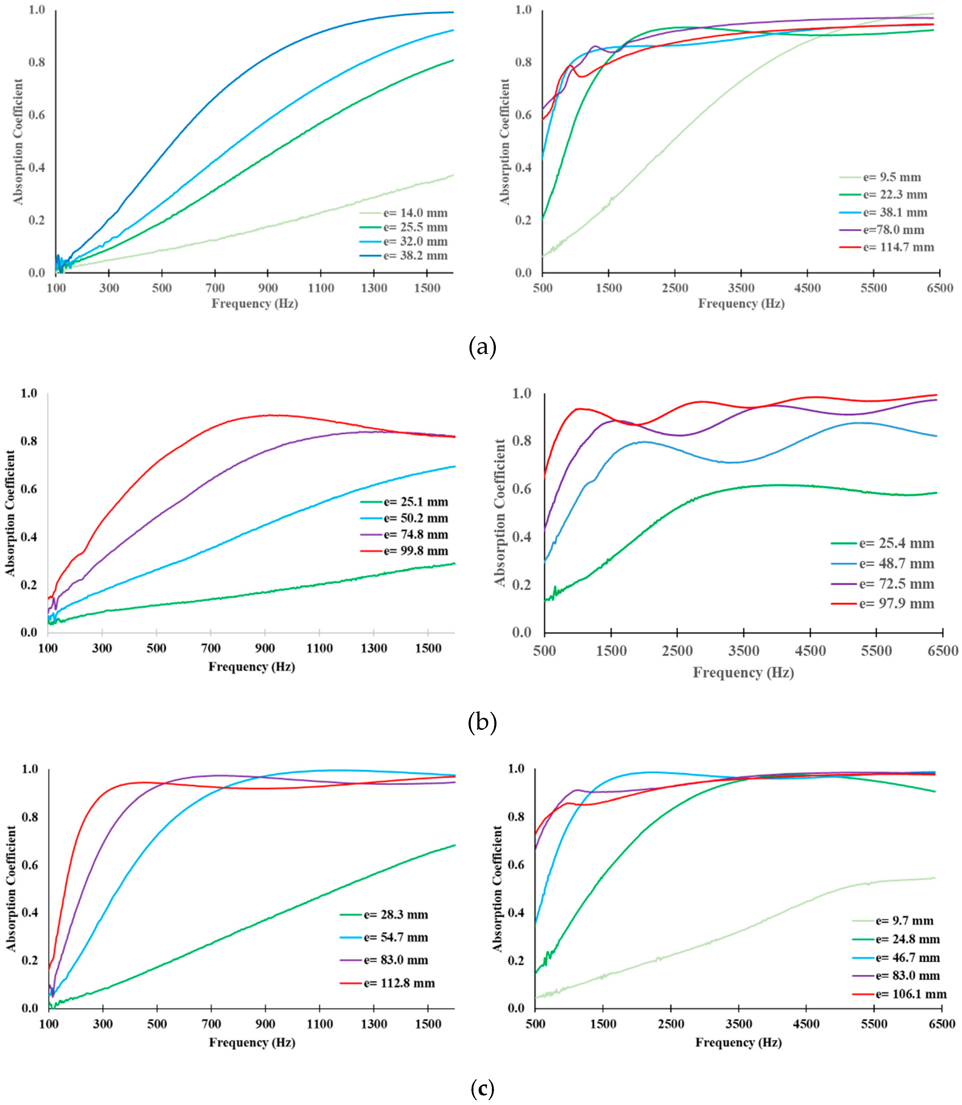
Figure 3 shows that the shape of the sound absorption spectrum changes markedly with sample thickness for all three materials and for both impedance tube diameters. These results are consistent with those shown in previous studies [26].
It is clear from Figure 3 that increasing the sample thickness affects not only the magnitude of the sound absorption coefficient but also the overall shape of its frequency response. In the case of the 100 mm samples, the spectrum for the thinnest samples is almost linear, increasing the curvature of the spectra with increasing thickness. In the case of the 29 mm samples, the spectra become increasingly complex as thickness increases.
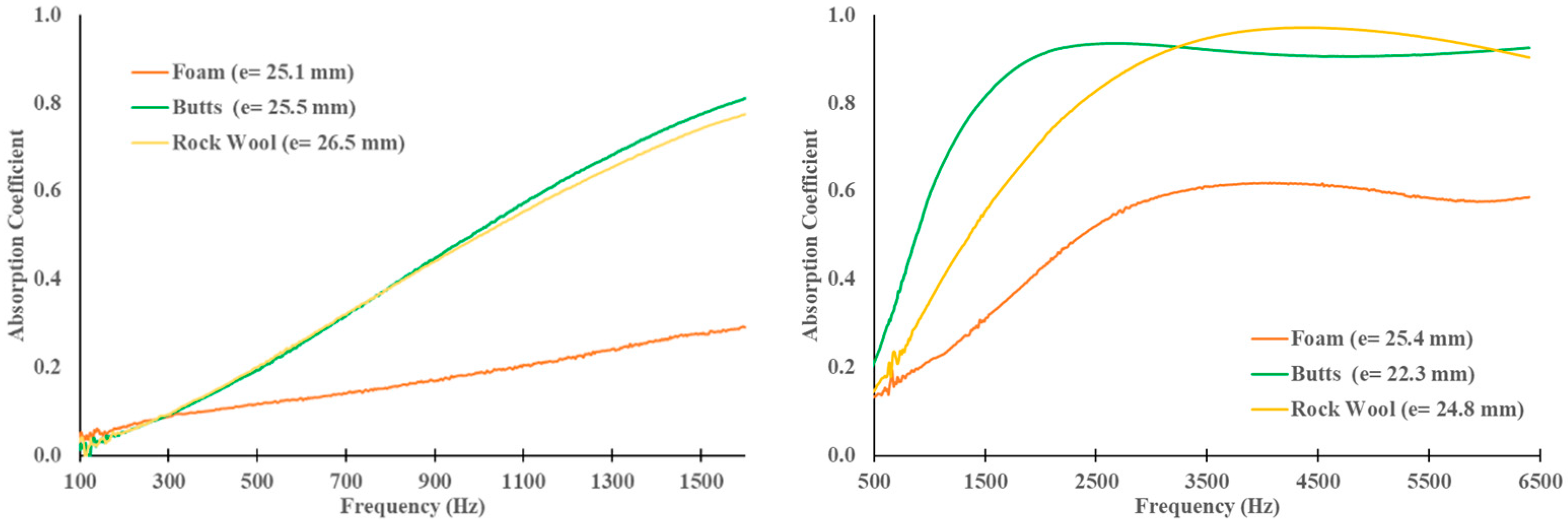
Figure 4 compares the three materials for similar sample thicknesses. As can be seen, in the 100 mm tube, the cigarette butt and mineral wool samples show similar spectral characteristics. In the 29 mm tube, although some similarity is also observed between the cigarette butt and mineral wool samples, greater variability is observed among the spectra of the types of samples. For both diameters, the spectra of the foam samples show a behavior that is quite different from the others.
These observations raise the question of whether the proposed theoretical models are valid for all thicknesses of the type of sample for which they were proposed and whether they could be applicable to other types of samples.
When sound absorption coefficients are measured using impedance tubes of different diameters, the acquisition system can combine the results into a single broadband spectrum.
However, this procedure is not always appropriate for the samples considered in this study. Unavoidable differences in sample preparation (for example, difficulty in reproducing exactly the same porous structure) may produce discrepancies between the measurements obtained with the 29 and 100 mm impedance tubes. As a result, the overlap region between the two spectra (approximately 1000–2000 Hz) may exhibit slight discontinuities. These differences were observed mainly in butts-derived and mineral wool samples.
Nevertheless, spectra from samples with similar thicknesses were combined and included in the analysis.
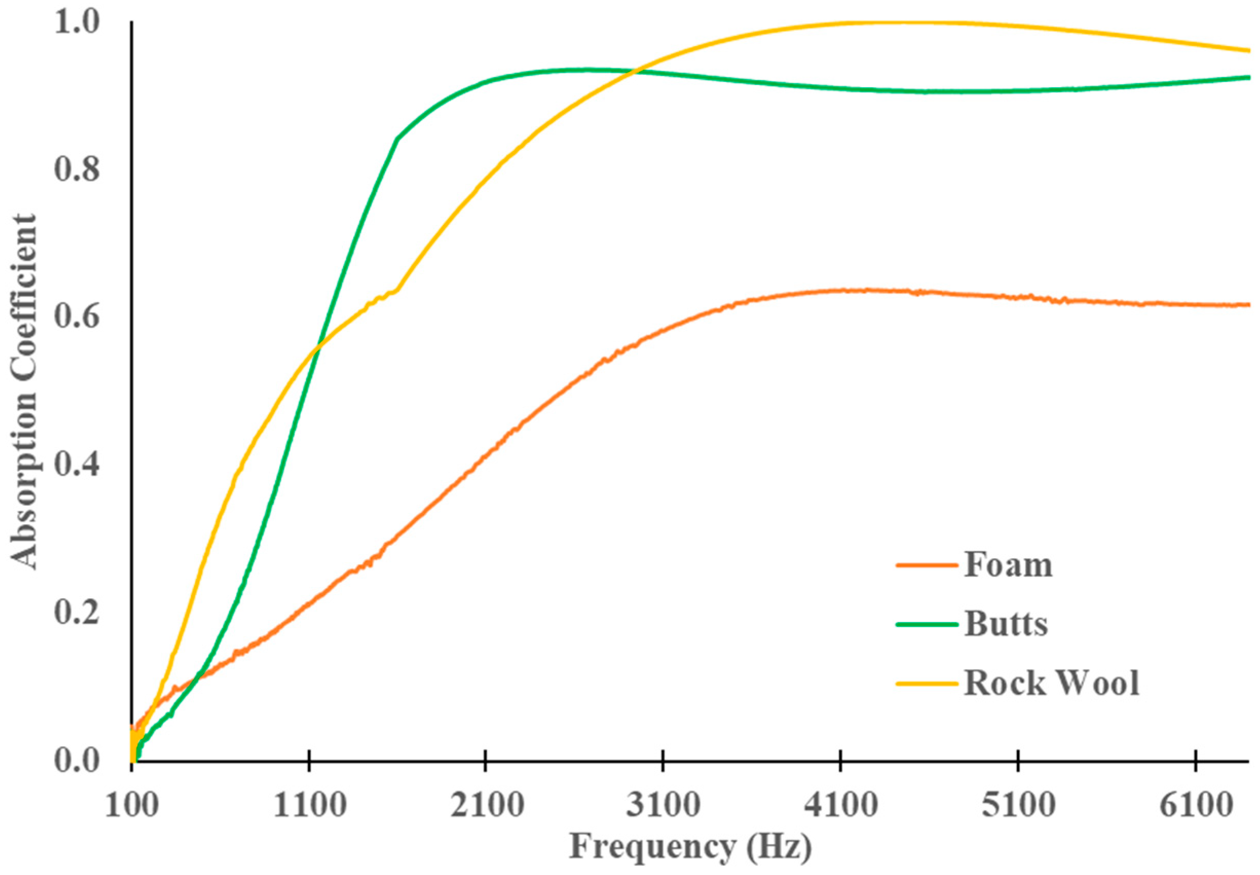
Figure 5 presents representative combined spectra for the three materials considered, all with a thickness of approximately 25 mm. A slight discontinuity can be observed in the overlap region, particularly for the mineral wool sample.

3.2. Application of the Different Proposed Theoretical Models to the Samples: 100 mm Tube Spectra

The performance of the ten theoretical models was first assessed using the spectra measured with the 100 mm impedance tube (100–1600 Hz). The RMSE values obtained for each sample are summarized in Table 3.
For the recycled cigarette butt samples, model M9 provided the lowest RMSE values for most samples thicker than 25 mm (except one case where model M10 provided the lowest value). For thinner samples, the best agreement was shared among models M7, M8, M9 and M10. For the foam samples, model M6 consistently provided the lowest RMSE values over most of the thickness range, whereas model M2 performed better only for the thickest samples (approximately 100 mm). In the case of mineral wool samples, models M7, M9 and M10 provided the best agreement for thicknesses above 50 mm. For thinner samples, model M10 led to better RMSE values, except in one case, which was model M5.
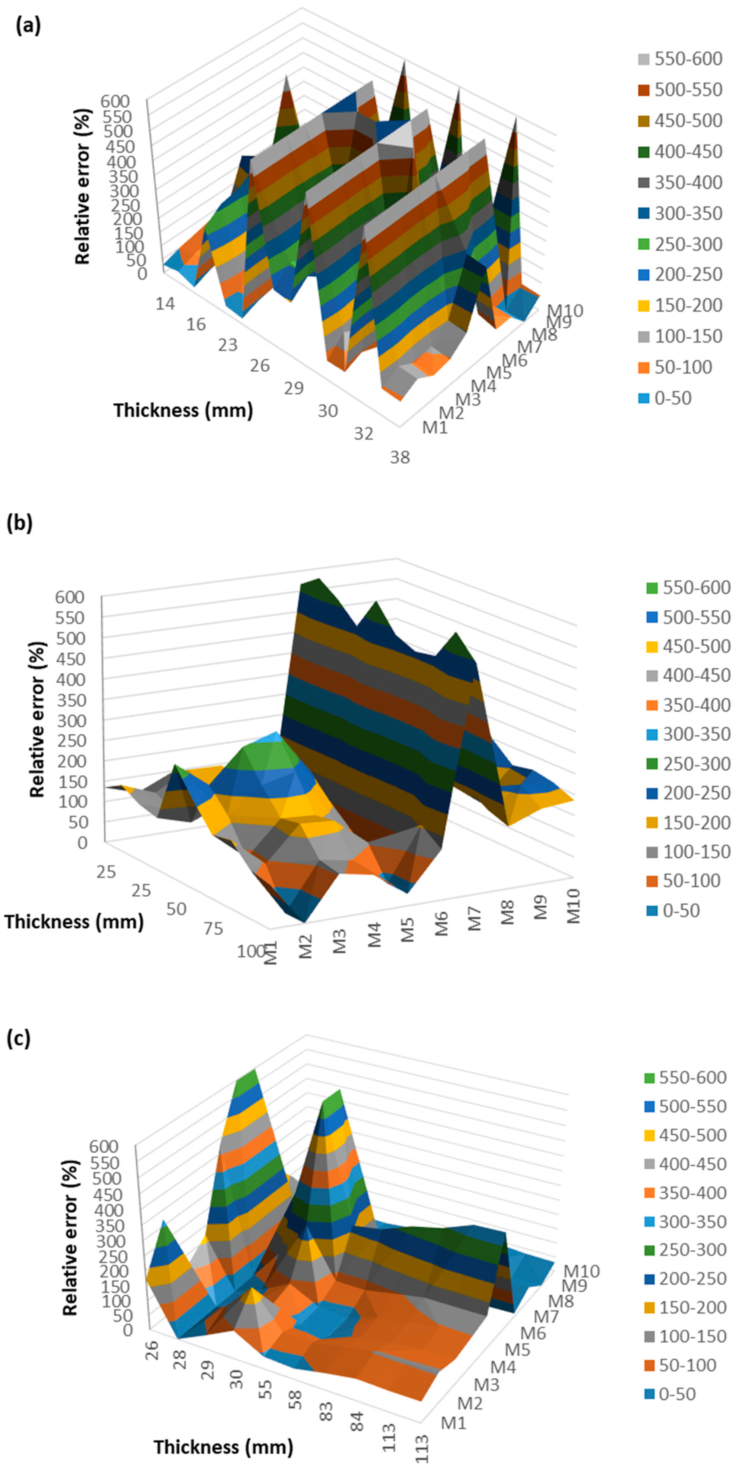
To complement the analysis based solely on the minimum RMSE values, the relative RMSE values [Equation (9)] were also calculated, allowing the performance of models with similar fitting accuracy to be compared. The relative RMSE values for all samples and models are presented in Figure 6, whereas the corresponding mean relative RMSE values, grouped according to material type and sample thickness, are summarized in Table 4.
Considering the overall results (row all in Table 4), model M9 provided the lowest mean relative RMSE values for the recycled cigarette butt samples. However, when the influence of sample thickness is taken into account, a more complex behavior is observed. For samples with thicknesses between 10 and 20 mm, model M7 yielded the lowest mean relative RMSE values. This result is consistent with the marked differences observed in the sound absorption spectra of the thinnest samples (Figure 3a). For samples thicker than 20 mm, model M9 consistently provided the best overall agreement, whereas the remaining models generally exhibited mean relative RMSE values exceeding 200%, indicating a substantially poorer fit.
For the foam samples, model M6 yielded the lowest overall mean relative RMSE value (Table 4). The same trend was observed for samples up to approximately 80 mm thick. Only for the thickest samples (around 100 mm) did model M2 outperform the remaining formulations. For all other models, the mean relative RMSE values were generally more than 100% higher than those of the best-performing model.
For the mineral wool samples, model M9 provided the lowest overall mean relative RMSE value and was also the best-performing model in three of the four thickness intervals considered. The only exception corresponded to the 75–100 mm interval, for which model M7 yielded the lowest mean relative RMSE. However, the results for the 25–50 mm interval were strongly influenced by sample MW100-2, for which model M2 produced a substantially lower RMSE than any other formulation. Because this single sample had a pronounced effect on the mean values reported in Table 4, an additional analysis was performed excluding this apparent outlier. The corresponding results are summarized in Table 5.
After excluding sample MW100-2, model M10 provided the lowest overall mean relative RMSE for the mineral wool samples (Table 5). Nevertheless, the optimal model still depended on sample thickness. Model M10 performed best for samples thinner than 50 mm, model M9 yielded the lowest mean relative RMSE values for the 50–75 mm and 100–125 mm intervals, and model M7 was the best-performing model for samples with thicknesses between 75 and 100 mm.
The results presented in this section indicate that foam requires different empirical models from those that best describe recycled cigarette butt and mineral wool samples, which is consistent with its cellular structure compared with the fibrous nature of the other two materials. Furthermore, these results indicate that no single Delany–Bazley-derived formulation provides the best prediction over the entire thickness range. Even for the same material, the optimal model depends strongly on sample thickness.

3.3. Application of the Different Proposed Theoretical Models to the Samples: 29 mm Tube Spectra

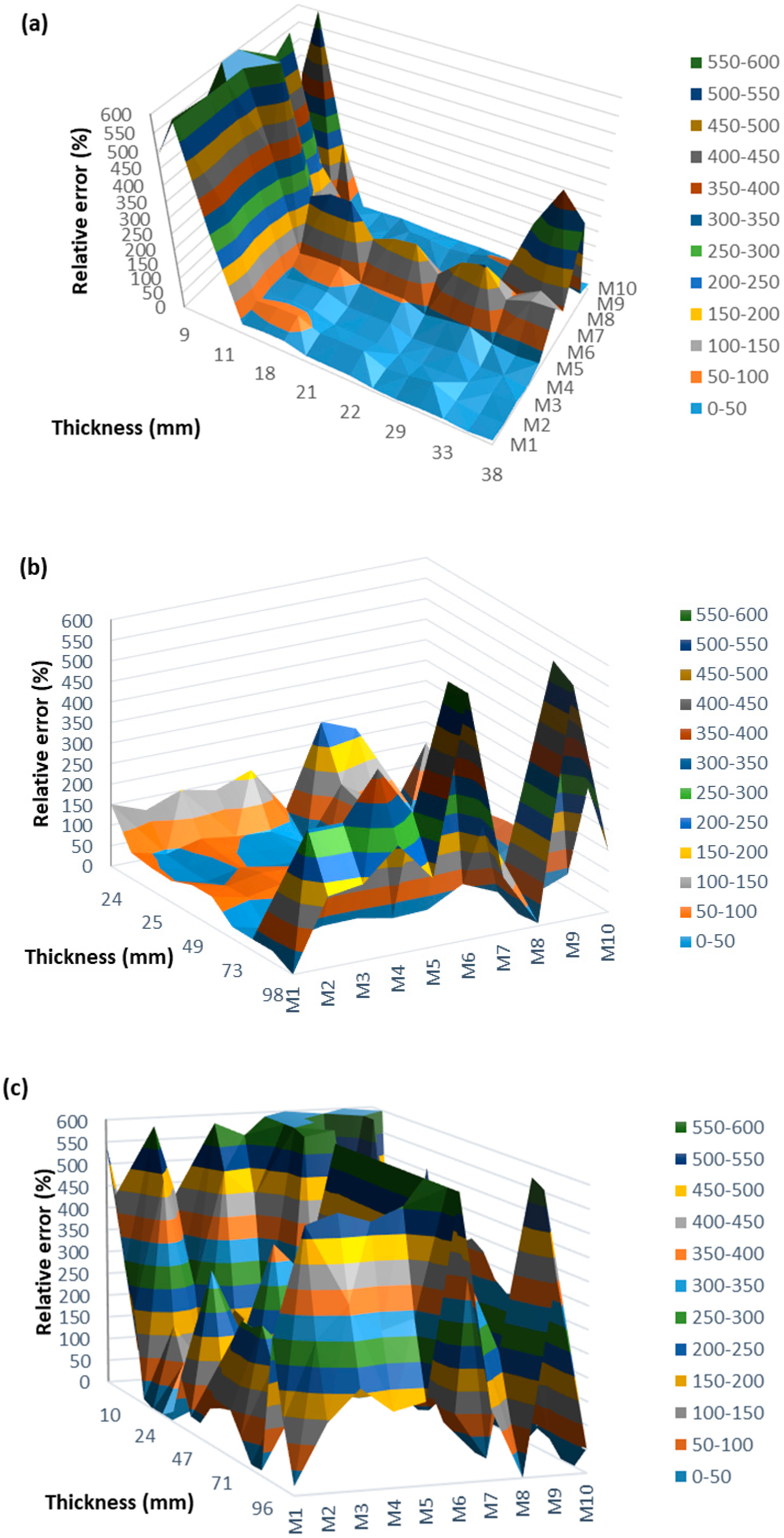
The results obtained with the 29 mm impedance tube, corresponding to the frequency range 500–6400 Hz, are summarized in Table 6 and Table 7 and Figure 7. As previously shown in Figure 3, the shape of the sound absorption spectrum changes markedly with sample thickness, suggesting that the suitability of the empirical models may also depend on this parameter.
For the recycled cigarette butt samples, model M9 clearly provided the best agreement for the thinnest individual samples (thicknesses below 11 mm). Moreover, in the 5–20 mm thickness interval, this model is clearly the best, whereas the remaining models yielded relative RMSE values generally exceeding 150%. For thicker samples, however, the differences among most of the models became much less pronounced. Only models M6 and, for the thickest samples, M8 consistently exhibited poorer performance. Within the intermediate thickness range (20–30 mm), models M8 and M10 provided the lowest RMSE values, whereas model M4 performed best for samples between 30 and 40 mm thick. These trends are also evident in Figure 7a.
Considering individual foam samples, model M6 consistently provided the lowest RMSE values for samples up to approximately 50 mm thick. For the thickest samples (around 100 mm), however, models M1 and M8 yielded the best agreement with the experimental measurements. The analysis of the mean relative RMSE values confirms this trend: model M6 performed best for the 20–40 mm and 40–60 mm thickness intervals, whereas models M9 and M8 provided the lowest mean relative RMSE values for the 60–80 mm and 80–100 mm intervals, respectively. In the latter interval, all the remaining formulations, except model M1, exhibited relative RMSE values generally exceeding 125%. Nevertheless, for samples between 25 and 75 mm thick, models M1, M2, M3, M4, M8 and M10 all produced relative RMSE values within 50% of the minimum, indicating that several empirical formulations provide similarly accurate predictions for acoustic foam over this thickness range.
A markedly different behavior was observed for mineral wool samples. Except for the two thinnest samples (approximately 10 mm thick), whose sound absorption spectra differ substantially from those of the thicker samples (Figure 3), model M10 consistently yielded the lowest RMSE values. For the two thinnest samples, model M5 provided the best agreement, whereas model M8 also produced the lowest RMSE values for some samples thicker than 75 mm. Interestingly, model M6, which consistently performed best for the acoustic foam samples, showed one of the poorest performances for mineral wool, highlighting the strong influence of the porous structure on the suitability of the empirical models.
Considering the overall results (row all in Table 7), models M9, M1 and M10 provided the lowest mean relative RMSE values for the recycled cigarette butt, foam and mineral wool samples, respectively. However, these overall results should be interpreted with caution, since, as drawn in the previous section, sample thickness plays a more important role than expected in determining the suitability of each empirical formulation.

3.4. Application of the Different Proposed Theoretical Models to the Samples: Combined Spectra

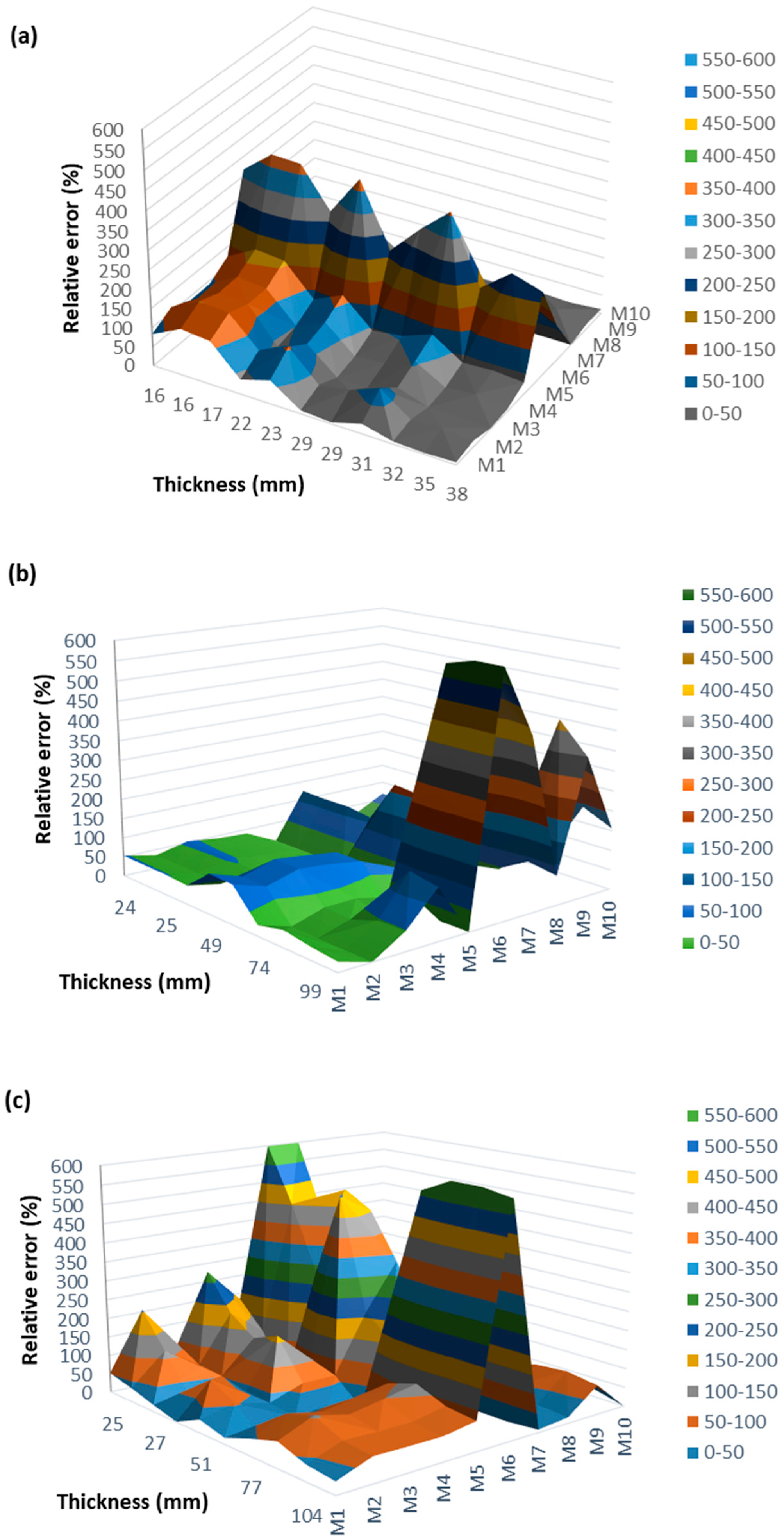
The results obtained from the combined spectra, covering the frequency range from 100 to 6400 Hz, are summarized in Table 8. The corresponding relative RMSE values are presented in Figure 8, whereas the mean relative RMSE values, grouped according to material type and sample thickness, are summarized in Table 9.
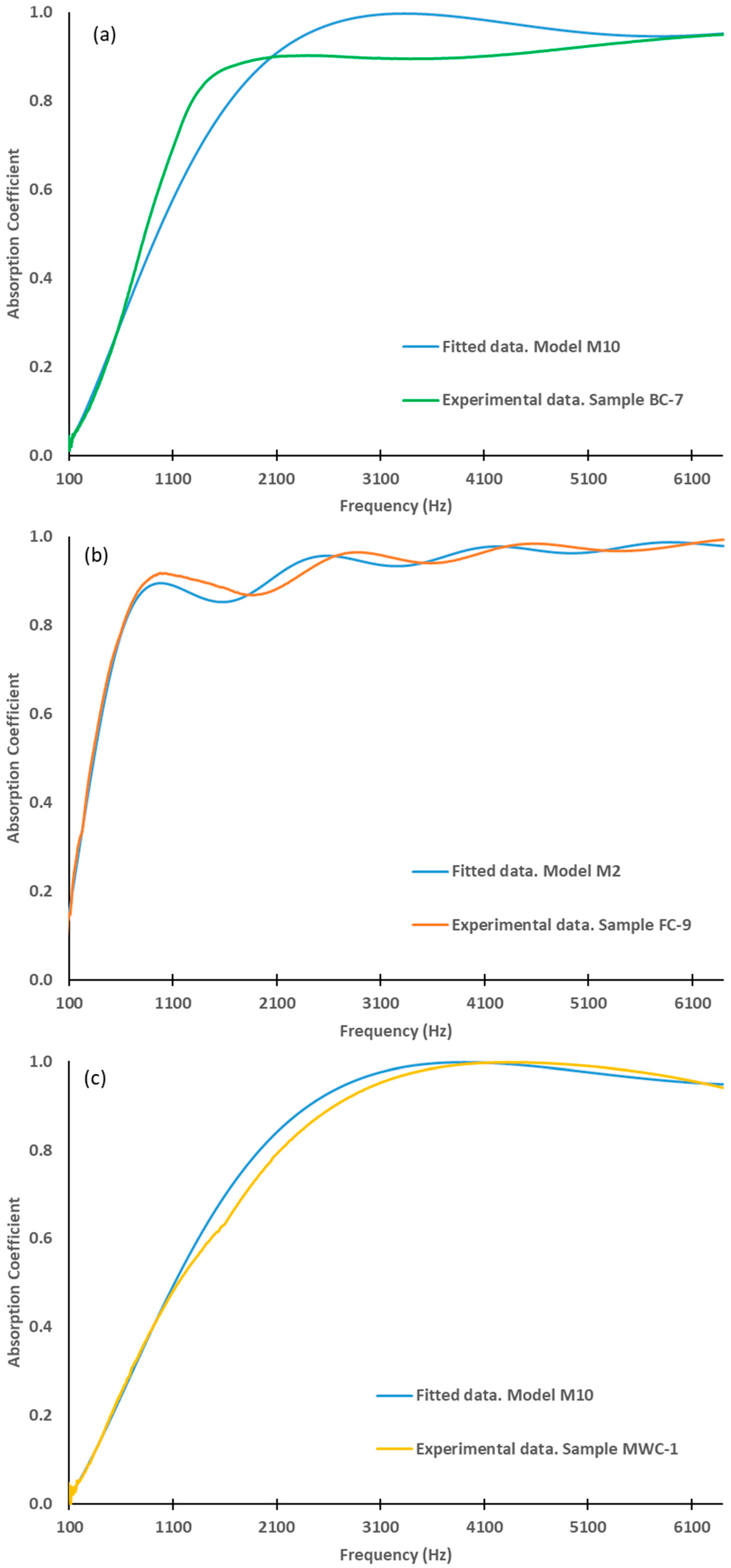
For the recycled cigarette butt samples, model M9 yielded the lowest RMSE values for the thinnest samples, whereas models M8 and M10 provided the best agreement as sample thickness increased. The minimum RMSE value was obtained with model M10 for sample BC7 [Figure 9a].
For the foam samples, the optimal model also depends on sample thickness. Model M6 consistently performed best for samples thinner than approximately 50 mm, whereas models M9 and, particularly, M2 provided the lowest RMSE values for thicker samples. The minimum RMSE value was obtained with model M2 for sample FC9 [Figure 9b].
The mineral wool samples exhibited more complex behavior. Models M5, M8 and M10 yielded the lowest RMSE values for the thinnest samples, whereas models M2 and M10 performed best for intermediate thicknesses (50–70 mm). For samples thicker than 70 mm, models M10 and, particularly, M7 provided the best agreement. The minimum RMSE value was obtained with model M10 for sample MWC-1 [Figure 9c].
The analysis of the mean relative RMSE values (Table 9) confirms the strong influence of sample thickness on model performance. For the recycled cigarette butt samples, model M9 clearly outperformed the remaining formulations for thicknesses below 20 mm, whereas several models provided comparable results for thicker samples, with the exception of models M5 and M6, which consistently exhibited poorer performance. Interestingly, model M8, which showed limited accuracy for the individual 29 mm and 100 mm measurements in the 30–40 mm thickness range, provided the best overall performance for the corresponding combined spectra.
For the foam samples, model M6 yielded the lowest mean relative RMSE values for thicknesses below 60 mm, whereas model M2 consistently performed best for thicker samples. Model M5 also provided competitive results for samples between 80 and 100 mm thick.
For the mineral wool samples, models M10 and M1 performed best for the thinnest samples (0–25 mm and 25–50 mm, respectively), model M8 yielded the lowest mean relative RMSE values for samples between 50 and 75 mm thick, and model M7 clearly outperformed the remaining models for samples in the two intervals thicker than 75 mm.
The combined spectra confirm once again that model selection cannot be based solely on the type of material, as it depends on the thickness of the sample.

3.5. Comparison of the Results Obtained for the Different Spectrum Types

In the previous section, the results obtained for the three spectrum types (100 mm spectra, 29 mm spectra, and combined spectra) were presented. Table 10 compares the RMSE values obtained for each spectrum type, material, and thickness range.
As shown in Table 10, for recycled cigarette butt and foam samples, the lowest RMSE values for the thinnest samples (<20 and 20–40 mm, respectively) were generally obtained using the 100 mm spectra for almost all models, with the exception of model M9 for cigarette butt samples and model M6 for foam samples.
The combined spectra only provided better results in isolated cases for cigarette butt samples. In contrast, they outperformed the other spectrum types in almost all thickness ranges for foam samples, and for most models within the 25–50 mm thickness range for mineral wool samples.
The models yielding the lowest RMSE values are consistent with those identified in the previous section. For recycled cigarette butt samples, model M9 most frequently produced the lowest RMSE values (five cases), while the remaining minimum values were obtained with models M4, M7, and M8 (one, one, and two cases, respectively).
For foam samples, model M6 clearly provided the best performance in the first two thickness intervals (20–40 and 40–60 mm). For thicker samples, model M2 most frequently produced the lowest RMSE values (three cases), while the remaining minimum values were shared among models M6, M8, and M9 (one case each).
Finally, for mineral wool samples, model M10 produced the lowest RMSE values for the thinnest samples (0–25 mm and 25–50 mm ranges), accounting for three cases. The remaining cases were obtained with models M1 and M2 (one case each). For the thicker samples, the minimum RMSE values were distributed among models M5 (one case), M7 (three cases), M9 (two cases), and M10 (three cases).

4. Conclusions

The main conclusions of the present study can be summarized as follows:
Increasing sample thickness significantly modifies not only the magnitude of the sound absorption coefficient but also the overall shape of the sound absorption spectrum. As a consequence, the most suitable empirical model depends not only on the porous material but also on sample thickness and the frequency range considered. Thus, no single model consistently provided the best agreement over the entire thickness range for any of the materials investigated.
The models yielding the lowest mean relative RMSE values for each material, frequency range and thickness interval are summarized in Table 11.
Foam samples exhibited a behavior clearly different from that of the fibrous materials investigated. Models M2 and, particularly, M6 provided the best agreement for most of the foam samples, whereas model M6 consistently performed poorly for the fibrous materials. This result is noteworthy because model M6 was originally proposed for kenaf fiber materials, highlighting that the suitability of these empirical models cannot be inferred solely from the material for which they were originally developed.
For the recycled cigarette butt samples, model M9 provided the best overall performance for the 100 mm impedance tube and for the thinner specimens analyzed using the 29 mm tube and the combined spectra. This agreement is particularly interesting because cigarette filters are composed primarily of cellulose acetate, whereas model M9 was originally developed for cellulose-based materials.
For the mineral wool samples, the most suitable empirical model depended strongly on both sample thickness and frequency range. Model M9 generally provided the best agreement in the 100–1600 Hz frequency range, whereas models M1, M7, M8 and M10 became more suitable for the higher-frequency analyses depending on the sample thickness.
Overall, the present results are consistent with recent validation studies while extending their practical implications. Recent investigations have shown that the prediction accuracy of Delany–Bazley-type empirical models depends on the porous material considered and that no single formulation provides uniformly accurate predictions for all absorber types. Consequently, previous authors have generally recommended either material-specific empirical models or the calibration of model coefficients for the material under investigation [3,33]. Likewise, the comprehensive review by Devi et al. highlighted that different empirical and semi-phenomenological models exhibit different levels of accuracy depending on the porous medium and recommended validating model predictions against experimental measurements whenever possible.
The present study confirms these observations for fibrous absorbers, where the best-performing formulations generally correspond to models originally developed for fibrous materials. However, the systematic comparison performed here also reveals that material type alone is insufficient to identify the most appropriate empirical model due to the influence of thickness. Model M6, originally proposed for kenaf fiber materials, provided the best overall performance for foam samples, whereas model M9 yielded the lowest prediction errors for recycled cigarette butt absorbers despite having been developed for cellulose-based materials.
Therefore, Delany–Bazley-type empirical models should not be selected solely according to the material category for which they were originally proposed. Instead, both the material characteristics, sample thickness, and the frequency range should be considered, with the overall shape of the measured sound absorption spectrum serving as a practical criterion for model selection.
The novelty of the present work does not lie in the development of a new empirical model, but in the systematic comparison of ten Delany–Bazley-based formulations across different porous materials, sample thicknesses and frequency ranges and impedance tube configurations. This comparison provides a practical framework for selecting the most appropriate empirical model for both conventional and recycled porous absorbers under different experimental conditions.
Finally, further studies involving additional porous materials with different microstructural characteristics would be valuable to assess the generality of the trends identified in the present work.

Author Contributions

C.M.G. performed all the sample measurements. V.G.E. implemented theoretical equations in spreadsheet software. All the authors contributed in a similar way in the original drafting preparation and in the review and editing of the final document. All authors have read and agreed to the published version of the manuscript.

Funding

This work was partially supported by Altadis Imperial Brands (Project 075/21). The funder was not involved in the study design, collection, analysis, interpretation of data, the writing of this article or the decision to submit it for publication.

Data Availability Statement

The original contributions presented in this study are included in the article. Further inquiries can be directed to the corresponding author.

Acknowledgments

This work was partially supported by Altadis Imperial Brands (Project 075/21), by the European Regional Development Fund (ERDF), and Fondo Social Europeo Plus (FSE+) through “Ayudas para la contratación de personal investigador predoctoral en formación por el Sistema Extremeño de Ciencia, Tecnología e Innovación” (PD23008). Thanks also to Carmen Mª Ortiz Caraballo for helping in the development of the acoustical model’s implementation.

Conflicts of Interest

The authors declare that this study received funding from Altadis (Imperial Tobacco). The funder was not involved in the study design, collection, analysis, interpretation of data, the writing of this article or the decision to submit it for publication. The remaining authors declare no conflicts of interest.

References

  1. Arenas, J.P.; Crocker, J.P. Recent Trends in Porous Sound-Absorbing Materials. J. Sound Vib. 2010, 44, 12–17. [Google Scholar]
  2. Egab, L.; Wang, X.; Fard, M. Acoustical characterization of porous sound absorbing materials: A review. Int. J. Veh. Noise Vib. 2014, 10, 129–149. [Google Scholar] [CrossRef]
  3. Devi, A.; Gautam, C.; Garg, N. Experimental and Analytical Evaluation of Models for Predicting Sound Absorption Characteristics of Acoustical Materials. MAPAN J. Metrol. Soc. India 2025, 40, 557–585. [Google Scholar] [CrossRef]
  4. Delany, M.E.; Bazley, E.N. Acoustical properties of fibrous absorbent materials. Appl. Acoust. 1970, 3, 105–116. [Google Scholar] [CrossRef]
  5. Kidner, M.R.; Hansen, C.H. A comparison and review of theories of the acoustic absorption of porous materials. Int. J. Acoust. Vib. 2008, 13, 112–119. [Google Scholar]
  6. Berardi, U.; Iannace, G. Acoustical characterization of natural fibers for sound absorption applications. Build. Environ. 2015, 94, 840–852. [Google Scholar] [CrossRef]
  7. Martellotta, F.; Cannavalea, A.; Matteisb, V.; Ayra, U. Sustainable sound absorbers obtained from olive pruning wastes and chitosan binder. Appl. Acoust. 2018, 141, 71–78. [Google Scholar] [CrossRef]
  8. Raj, M.; Fatima, S.; Tandon, N. Recycled materials as a potential replacement to synthetic sound absorbers: A study on denim shoddy and waste jute fibers. Appl. Acoust. 2020, 159, 107070. [Google Scholar] [CrossRef]
  9. Maderuelo-Sanz, R. Characterizing and modelling the sound absorption of the cellulose acetate fibers coming from cigarette butts. J. Environ. Health Sci. Eng. 2021, 19, 1075–1086. [Google Scholar] [CrossRef] [PubMed]
  10. Aygun, H.; Gómez-Agustina, L.; Mundula, S. Acoustic wave propagation through eco-friendly porous panels at normal incidence. Build. Acoust. 2023, 30, 359–372. [Google Scholar] [CrossRef]
  11. Dunn, I.P.; Davern, W.A. Calculation of Acoustical Impedance of Multi-layer Absorbers. Appl. Acoust. 1986, 19, 321–334. [Google Scholar] [CrossRef]
  12. Wu, Q. Empirical relations between acoustical properties and flow resistivity of porous plastic open-cell foam. Appl. Acoust. 1988, 25, 141–148. [Google Scholar] [CrossRef]
  13. Miki, Y. Acoustical properties of porous materials–Modifications of Delany-Bazley models-. J. Acoust. Soc. Jpn. E 1990, 11, 19–24. [Google Scholar] [CrossRef]
  14. Garai, M.; Pompoli, F. A simple empirical model of polyester fibre materials for acoustical applications. Appl. Acoust. 2005, 66, 1383–1398. [Google Scholar] [CrossRef]
  15. Ramis, J.; Alba, J.; Rey, R.; Escuder, E.; Sanchís, V.J. New absorbent material acoustic based on kenaf’s fibre. Mater. Constr. 2010, 60, 133–143. [Google Scholar] [CrossRef]
  16. Arenas, J.P.; Rebolledo, J.; Rey, R.; Alba, J. Sound absorption properties of unbleached cellulose loose-fill insulation material. BioResources 2014, 9, 6227–6240. [Google Scholar] [CrossRef]
  17. Rey, R.; Uris, A.; Alba, J.; Candelas, P. Characterization of sheep wool as a sustainable material for acoustic applications. Materials 2017, 10, 1277. [Google Scholar] [CrossRef] [PubMed]
  18. Dunne, R.K. A universal empirical model for materials in acoustic application. Appl. Acoust. 2025, 231, 110549. [Google Scholar] [CrossRef]
  19. Berardi, U.; Iannace, G. Predicting the sound absorption of natural materials: Best-fit inverse laws for the acoustic impedance and the propagation constant. Appl. Acoust. 2017, 115, 131–138. [Google Scholar] [CrossRef]
  20. Taban, E.; Valipour, F.; Abdi, D.D.; Amininasab, S. Mathematical and experimental investigation of sound absorption behavior of sustainable kenaf fiber at low frequency. Int. J. Environ. Sci. Technol. 2021, 18, 2765–2780. [Google Scholar] [CrossRef]
  21. Gómez Escobar, V.; Maderuelo-Sanz, R. Acoustical performance of samples prepared with cigarette butts. Appl. Acoust. 2017, 125, 166–172. [Google Scholar] [CrossRef]
  22. Gómez Escobar, V.; Rey Gozalo, G.; Pérez, C.J. Variability and Performance Study of the Sound Absorption of Used Cigarette Butts. Materials 2019, 12, 2584. [Google Scholar] [CrossRef] [PubMed]
  23. Xie, K.; Cao, Y.; He, Z.; Wang, K.; Ding, J.; MacGillivray, I.; Skvortsov, A.; Qiu, X.; Li, D. Acoustic absorption of ultralight graphene-based cellular monoliths. Appl. Phys. A 2022, 128, 896. [Google Scholar] [CrossRef]
  24. Gómez Escobar, V.; Moreno González, C.; Rey Gozalo, G. Analysis of the Influence of Thickness and Density on Acoustic Absorption of Materials Made from Used Cigarette Butts. Materials 2021, 14, 4524. [Google Scholar] [CrossRef] [PubMed]
  25. Hassan, T.; Jamshaid, H.; Mishra, R.; Khan, M.Q.; Petru, M.; Tichy, M.; Muller, M. Factors Affecting Acoustic Properties of Natural-Fiber-Based Materials and Composites: A Review. Textiles 2021, 1, 55–85. [Google Scholar] [CrossRef]
  26. Moreno González, C.; Gómez Escobar, V.; Pérez, C.J.; Rey Gozalo, G. Behavior of the First Absorption Peak of Porous Materials with Changing Thickness. Acoust. Aust. 2026, 54, 201–217. [Google Scholar] [CrossRef]
  27. ISO 10534-2; Acoustics: Determination of Sound Absorption Coefficient and Impedance in Impedances Tubes. Part 2: Transfer-Function Method. International Organization for Standardization: Geneva, Switzerland, 1998.
  28. Ingard, K.U.; Dear, T.A. Measurement of acoustic flow resistance. J. Sound. Vib. 1985, 103, 567–572. [Google Scholar] [CrossRef]
  29. Gómez Escobar, V.; Moreno González, C.; Arévalo Caballero, M.J.; Gata Jaramillo, A.M. Initial conditioning of used cigarette filters for their recycling as acoustical absorber materials. Materials 2021, 14, 4161. [Google Scholar] [CrossRef] [PubMed]
  30. Sanchis, E.J. Modelización, Simulación y Caracterización Acústica de Materiales Para su uso en Acústica Arquitectónica. Ph.D. Thesis, Universitat Politècnica de València, Valencia, Spain, 2008. [Google Scholar] [CrossRef]
  31. Attenborough, K. Acoustical characteristics of rigid fibrous absorbents and granular materials. J. Acoust. Soc. Am. 1983, 73, 785–799. [Google Scholar] [CrossRef]
  32. Oliva, D.; Hongisto, V. Sound absorption of porous materials-Accuracy of prediction methods. Appl. Acoust. 2013, 74, 1473–1479. [Google Scholar] [CrossRef]
  33. Alba, J.; Rodríguez, J.C.; del Rey, R. Review of the Delany and Bazley Empirical Model and Adjustment of New Coefficients for Open-Pore Foams. Acoustics 2025, 7, 62. [Google Scholar] [CrossRef]
Figure 1. Experimental configuration used for the sound absorption measurements.
Materials 19 03128 g001
Figure 2. Representative photographs of some of the samples with a 100 mm diameter. (a) sample prepared with used cigarette butts; (b) foam sample; (c) commercial mineral wool sample.
Materials 19 03128 g002
Figure 3. Sound absorption coefficient spectra of representative samples used cigarette butt (a), foam (b) and mineral wool (c) samples with different thicknesses measured using the two impedance tube diameters [left: 100 mm; right: 29 mm].
Materials 19 03128 g003
Figure 4. Sound absorption coefficients for some examples of samples of different types with similar thickness, measured using the two impedance tube diameters [(left): 100 mm; (right): 29 mm].
Materials 19 03128 g004
Figure 5. Sound absorption coefficients for combined spectra of the different types of samples with similar thickness (near 25 mm).
Materials 19 03128 g005
Figure 6. Relative RMSE values for 100 mm samples [(a) used cigarette butts; (b) foam; (c) mineral wool].
Materials 19 03128 g006
Figure 7. Relative RMSE values for 29 mm samples [(a) used cigarette butts; (b) foam; (c) mineral wool].
Materials 19 03128 g007
Figure 8. Relative RMSE values for combined samples [(a) used cigarette butts; (b) foam; (c) mineral wool].
Materials 19 03128 g008
Figure 9. Measured spectra and fitted data for the minimum RMSE values calculated for combined spectra. [(a) used cigarette butts; (b) foam; (c) mineral wool].
Materials 19 03128 g009
Table 1. Number of samples and range of thicknesses of the samples measured.
Diameter of the SamplesType of SampleNumber of
Samples
Range of
Thicknesses (mm)
29 mmUsed cigarette butts158.8–38.1
29 mmFoam1023.9–97.9
29 mmMineral wool209.7–106.1
100 mmUsed cigarette butts1514.0–38.2
100 mmFoam1024.8–99.8
100 mmMineral wool1026.2–112.8
Table 3. RMSE values calculated for each model using the measurements performed with the 100 mm impedance tube. Shaded cells indicate the lowest RMSE value for each sample. B, F and MW denote samples made from recycled cigarette butts, foam and mineral wool, respectively.
SampleThickness
(mm)
M1M2M3M4M5M6M7M8M9M10
B100-0114.040.1000.1160.1260.1380.1430.2540.0770.0860.1420.097
B100-0216.050.1100.1270.1380.1510.1570.2790.0780.0930.1690.104
B100-0316.290.0890.1070.1170.1300.1370.2670.0910.0740.1770.083
B100-0417.780.1890.2100.2160.2340.2430.4010.1270.1650.0500.179
B100-0523.330.1120.1390.1360.1560.1740.3820.1690.0930.1490.087
B100-0624.580.1340.1580.1690.1790.1920.3650.1230.1180.2590.110
B100-0725.510.1780.2080.1870.2130.2430.4660.2070.1440.0140.144
B100-0825.530.1830.2140.2040.2260.2500.4780.1760.1540.0600.152
B100-0929.060.2070.2410.2070.2300.2730.4950.2160.1690.0700.165
B100-1029.890.1420.1780.1420.1590.2060.4260.2580.1170.0140.100
B100-1130.480.1050.1400.1160.1310.1700.4200.2380.0920.1200.062
B100-1231.150.2500.2850.2440.2640.3140.5230.2050.2080.1460.207
B100-1332.040.2180.2550.2290.2460.2880.5450.1980.1850.0130.170
B100-1433.990.2320.2700.2270.2410.2970.5160.2140.1950.1180.186
B100-1538.210.2390.2780.2320.2430.3030.5300.2030.2020.1230.189
F100-124.750.2470.2210.2590.2570.2010.1050.7020.2930.2100.279
F100-224.860.2310.2040.2420.2410.1850.0880.6860.2760.1940.276
F100-325.070.2490.2220.2610.2600.2030.1050.7000.2940.2130.281
F100-425.150.2590.2310.2700.2690.2120.1150.7100.3030.2220.291
F100-549.610.2350.1960.2450.2610.1950.0620.5090.2540.2240.266
F100-650.220.2570.2180.2670.2830.2170.0830.5250.2760.2430.288
F100-774.760.1480.1080.1560.1530.1150.0590.3610.1680.1340.180
F100-874.970.1520.1120.1600.1570.1190.0580.3630.1730.1370.184
F100-999.830.0780.0360.0770.0720.0470.0930.2590.0970.1150.112
F100-1099.830.0830.0410.0820.0760.0520.0900.2630.1010.1130.116
MW100-126.160.0540.0840.0420.0530.1050.2340.4070.0620.0470.020
MW100-228.320.0570.0380.0720.0660.0070.1270.4970.1190.0640.095
MW100-328.510.1160.1470.1030.1090.1680.2970.3690.0940.1170.079
MW100-429.810.0770.1120.0660.0740.1320.2880.3600.0720.0470.039
MW100-554.670.2300.2700.2220.2300.2880.5150.1690.1930.1630.179
MW100-658.130.1950.2360.1860.1930.2510.4750.1770.1610.1510.143
MW100-782.990.2220.2640.2250.2400.2770.5280.1420.1880.1560.173
MW100-884.290.2350.2750.2380.2540.2890.5360.1360.2000.1620.191
MW100-9112.80.2240.2680.2440.2620.2810.5720.1410.1950.1320.176
MW100-10112.80.2220.2660.2420.2590.2790.5710.1440.1930.1310.171
Table 4. Mean relative RMSE values for each model and material type obtained from measurements performed with the 100 mm impedance tube, grouped according to sample thickness. Shaded cells indicate the lowest mean relative RMSE value for each material/thickness group. B, F and MW denote samples made from recycled cigarette butts, foam and mineral wool, respectively.
TypeThickness
Interval (mm)
M1M2M3M4M5M6M7M8M9M10
All319.2396.4345.9392.0474.21001.5378.5250.342.8233.3
B10–2091.6118.9131.7153.7164.0361.843.764.485.581.9
20–30420.1523.9446.2514.9628.21334.2602.6327.134.4302.7
30–40380.0465.5396.9435.1537.51114.0377.4307.018.8271.2
All158.1101.1167.8167.6101.427.6578.1197.5152.7209.1
20–40139.9113.5151.3149.894.90.0582.9183.9104.0174.9
F40–60244.2189.5258.7281.0187.60.0626.8270.5227.2288.1
60–80157.189.2170.5165.3100.70.0519.6192.0131.6211.4
80–100109.30.0107.492.228.9138.0578.1157.4196.6196.4
All135.4154.3147.0153.8136.5532.3994.1205.8102.9134.5
25–50251.8254.5275.0277.6194.9909.72473.9463.1248.6302.2
MW50–7538.865.833.538.076.3224.713.915.72.95.1
75–10064.593.666.677.5103.5282.40.039.414.230.7
100–12569.9103.085.198.3112.9335.18.847.70.032.1
AllAll220.6242.9238.2259.8271.2589.2611.4222.591.4198.2
Table 5. Mean relative RMSE for the mineral wool samples measured using the 100 mm impedance tube after excluding sample MW100-2. Results are grouped according to sample thickness. Shaded cells indicate the lowest mean relative RMSE value for each thickness interval.
TypeThickness
Interval (mm)
M1M2M3M4M5M6M7M8M9M10
All73.3124.164.680.5151.7408.2353.257.626.715.1
25–50104.6197.370.398.9259.9663.21044.6104.468.60.0
MW50–7538.865.833.538.076.3224.713.915.72.95.1
75–10064.593.666.677.5103.5282.40.039.414.230.7
100–12569.9103.085.198.3112.9335.18.847.70.032.1
Table 6. RMSE values calculated for each model using the measurements performed with the 29 mm impedance tube. Shaded cells indicate the lowest RMSE value for each sample. B, F and MW denote samples made from recycled cigarette butts, foam and mineral wool, respectively.
SampleThickness
(mm)
M1M2M3M4M5M6M7M8M9M10
B29-18.780.3410.3790.3600.3750.4150.6900.2270.3030.0580.287
B29-29.480.3130.3530.3310.3420.3860.6700.2160.2750.0320.253
B29-310.750.3190.3620.3310.3390.3920.6830.2140.2790.0830.254
B29-416.040.1950.2360.1880.1950.2500.4690.1560.1620.1620.147
B29-517.710.1990.2400.1960.2040.2550.5000.1430.1640.1440.148
B29-618.450.1810.2200.1750.1850.2330.4540.1300.1490.1440.140
B29-720.970.1470.1710.1380.1460.1840.3090.1220.1250.1630.129
B29-821.560.1320.1590.1240.1350.1700.3090.1250.1100.1440.113
B29-922.310.1290.1560.1210.1340.1680.3130.1180.1080.1340.113
B29-1028.370.1010.1070.0970.0940.1200.2000.1300.0920.1220.098
B29-1128.670.0740.0870.0710.0750.0970.1980.1390.0690.1070.072
B29-1230.370.0830.1030.0800.0880.1110.2260.1150.0750.1200.074
B29-1333.460.0840.0810.0830.0750.0920.1640.1380.2750.1040.083
B29-1436.390.0650.0610.0660.0650.0700.1490.1370.3030.0920.065
B29-1538.060.0760.0710.0740.0660.0800.1650.1230.2790.0900.078
F29-123.880.3350.2940.3370.3140.3570.2080.4690.4240.1340.333
F29-223.990.3310.2900.3330.3090.2980.2040.4650.3490.2790.364
F29-324.630.3500.3090.3510.3270.3180.2270.4770.3660.2970.382
F29-425.440.3470.3060.3470.3210.3150.2290.4710.3620.2950.377
F29-548.620.2070.1840.2030.1950.1880.1210.2660.2030.1500.211
F29-649.320.2180.1950.2140.2080.1980.1260.2760.2130.1570.221
F29-772.50.1170.0980.1150.1170.1010.1010.1480.1120.0910.122
F29-873.310.1200.1010.1180.1200.1040.1080.1510.1160.0940.125
F29-997.940.0140.0450.0450.0580.0440.4890.0370.0110.1160.041
F29-1097.940.0170.0470.0490.0620.0460.4890.0400.0180.1150.043
MW29-19.690.2630.0680.1050.0970.0410.2350.3640.1560.3080.166
MW29-210.170.0710.0340.0710.0670.0130.2690.3320.1220.2630.133
MW29-323.090.0560.1030.0620.1030.0970.2710.1970.0490.1450.014
MW29-423.60.0500.0980.0580.1000.0900.2620.1980.0470.1430.017
MW29-524.480.0320.0780.0420.0860.0700.2410.1980.0390.1330.029
MW29-624.80.0310.0610.0480.0890.0470.2120.2170.0550.1350.059
MW29-734.650.0870.0940.1040.1290.0860.2580.2150.1030.1420.103
MW29-834.970.0620.0800.0790.1110.0720.2620.1890.0760.1290.073
MW29-946.690.0350.0730.0480.0810.0690.3010.0980.0320.1060.017
MW29-1049.280.0440.0770.0620.0930.0720.3110.1090.0440.1160.032
MW29-1156.860.0280.0650.0490.0740.0640.3440.0700.0270.0970.021
MW29-1259.450.0340.0700.0490.0740.0690.3590.0330.0270.0970.019
MW29-1371.490.0400.0750.0660.0830.0750.4330.0590.0370.1100.021
MW29-1472.880.0400.0760.0610.0760.0760.4370.0400.0330.1020.020
MW29-1581.660.0390.0750.0710.0820.0760.4860.0540.0350.1130.025
MW29-1683.050.0270.0620.0600.0670.0650.4870.0420.0240.1070.035
MW29-1795.970.0330.0690.0780.0730.0750.5670.0590.0290.1310.039
MW29-1895.970.0640.1010.1050.1010.1060.5910.0810.0550.1430.016
MW29-19106.140.0570.0950.1110.0970.1020.6340.0910.0480.1610.024
MW29-20106.140.0350.0720.0920.0760.0810.6170.0740.0300.1530.045
Table 7. Mean relative RMSE values for each model and material type obtained from measurements performed with the 29 mm impedance tube, grouped according to sample thickness. Shaded cells indicate the lowest mean relative RMSE value for each material/thickness group. B, F and MW denote samples made from recycled cigarette butts, foam and mineral wool, respectively.
TypeThickness
Interval (mm)
M1M2M3M4M5M6M7M8M9M10
All124.7153.2128.2135.1176.3396.2102.5162.625.890.2
B5–20291.2345.6306.4320.8384.1749.1170.0241.03.8215.5
20–3015.334.19.115.246.2165.333.10.434.94.8
30–4011.713.69.96.527.4155.388.0247.847.59.2
All54.683.3100.4113.788.7715.1132.459.7166.199.8
20–4079.857.980.367.572.613.9148.6101.824.190.2
F40–6071.953.168.763.156.30.0119.468.324.274.9
60–8027.87.826.028.210.913.061.323.50.033.5
80–10013.9240.0246.4342.2231.13534.5183.83.2757.8210.5
All123.0228.6196.3270.0211.91553.7476.7120.1513.573.2
0–25246.6265.4210.6340.7200.81162.91123.7273.4816.7216.6
25–5036.7128.982.8176.8113.7775.2270.943.2242.99.6
MW50–7575.1250.7175.2274.2247.21822.5145.251.3395.60.0
75–10093.7254.1262.1270.3270.42284.5172.670.2454.318.7
100–12579.6222.7291.2235.4253.62283.6218.251.6499.425.5
AllAll108.41171.20152.29190.33172.64981.47275.43120.85273.7384.79
Table 8. RMSE values calculated for each model using the combined spectra. Shaded cells indicate the lowest RMSE value for each sample. B, F and MW denote samples made from recycled cigarette butts, foam and mineral wool, respectively.
SampleThickness
(mm)
M1M2M3M4M5M6M7M8M9M10
BC116.170.2750.3190.2840.2870.3370.6260.2160.2380.1500.203
BC216.250.3100.3520.3260.3280.3740.6690.2370.2740.1400.241
BC316.880.3000.3430.3170.3170.3630.6630.2400.2630.1400.224
BC422.150.1570.1950.1560.1700.2040.4220.1530.1340.1130.123
BC523.450.1570.1990.1650.1790.2080.4630.1560.1330.0970.114
BC628.720.0930.1120.0900.1010.1230.2670.1530.0850.0900.092
BC729.280.0700.0970.0710.0860.1050.2660.1660.0680.0830.068
BC831.210.0920.1260.0950.1130.1330.3340.1410.0810.0930.073
BC932.310.0880.0970.0860.0920.1100.2360.1640.0820.0960.089
BC1035.190.0710.0830.0710.0820.0930.2380.1660.0680.0890.072
BC1138.140.0820.0900.0790.0820.1010.2500.1490.0770.0880.086
FC-124.370.3300.2910.3310.3090.2990.2160.4820.3460.2740.359
FC-224.520.3360.2970.3370.3150.3050.2210.4870.3520.2810.365
FC-324.750.3340.2950.3350.3130.3020.2200.4850.3490.2780.361
FC-425.260.3400.3010.3400.3150.3090.2310.4870.3550.2840.367
FC-549.120.1980.1710.1950.1850.1750.0990.3140.2010.1510.210
FC-649.770.2060.1800.2040.1960.1830.1040.3210.2090.1570.218
FC-773.630.1050.0840.1040.1050.0860.1280.2040.1080.0830.117
FC-874.140.0390.0270.0330.0300.0370.1860.1350.0400.0770.045
FC-998.890.0240.0180.0260.0440.0180.3560.1070.0340.0940.052
FC-1098.890.0260.0210.0310.0470.0210.3520.1090.0360.0920.053
MWC-124.880.0400.0800.0500.0990.0740.2200.2120.0370.1360.026
MWC-225.800.0530.0840.0610.1100.0830.2150.1990.0390.1380.043
MWC-326.560.0490.0530.0640.0990.0420.1600.2490.0730.1290.078
MWC-427.150.0370.0680.0490.0960.0660.2190.2000.0360.1270.044
MWC-550.680.0520.0600.0520.0640.0630.1230.1700.0410.1330.039
MWC-653.710.1370.1170.1440.1430.1190.2990.2400.1570.1470.170
MWC-777.240.1090.1380.1240.1350.1460.5050.0760.0930.1240.083
MWC-878.590.1150.1410.1270.1380.1500.5060.0690.0980.1260.094
MWC-9104.390.1120.1370.1340.1350.1470.6020.0790.0970.1500.096
MWC-10104.390.1190.1490.1470.1470.1590.6190.0970.1040.1590.090
Table 9. Mean relative RMSE values for each model and material type obtained from combined measurements, grouped according to sample thickness. Shaded cells indicate the lowest mean relative RMSE value for each material/thickness group. B, F and MW denote samples made from recycled cigarette butts, foam and mineral wool, respectively.
TypeThickness
Interval (mm)
M1M2M3M4M5M6M7M8M9M10
All43.071.646.056.584.3294.584.828.110.420.6
B<20106.1136.1116.1117.1150.1355.961.480.50.055.8
20–3028.162.629.444.873.4288.780.014.06.98.6
30–4010.732.19.922.845.9254.2107.22.821.86.3
All52.728.354.265.034.3412.2237.367.6116.492.7
20–4051.033.551.441.237.00.0118.858.025.963.6
F40–6099.473.696.988.476.90.0214.2102.752.3111.3
60–8034.30.724.218.920.0318.0271.338.591.552.2
80–10028.00.047.2135.40.71742.8463.480.9386.5172.8
All34.081.356.9115.281.1478.8251.625.9171.023.1
0–2551.8205.189.9276.2183.0737.5709.042.7419.60.0
25–5018.377.448.5160.965.3413.6453.824.8238.540.1
50–7525.226.627.242.131.7183.9219.119.6131.822.3
MW75–10054.892.873.388.1103.7596.70.032.372.622.5
100–12536.868.766.466.581.0624.13.718.883.010.4
AllAll43.2560.7652.1778.2067.16391.90187.8140.1096.4144.66
Table 10. Mean RMSE values for each model and material type according to sample thickness. Shaded cells indicate the lowest mean RMSE value for each model within each material/thickness group. Bold values indicate the lowest RMSE obtained for each spectrum type. B, F and MW denote samples made from recycled cigarette butts, foam and mineral wool, respectively.
TypeThickness
Interval (mm)
M1M2M3M4M5M6M7M8M9M10
100 mm0.1220.1400.1490.1630.1700.3000.0930.1040.1350.116
<2029 mm0.2580.2980.2630.2730.3220.5780.1810.2220.1040.205
Combined0.2950.3380.3090.3110.3580.6530.2310.2580.1430.223
100 mm0.1590.1900.1740.1940.2230.4350.1920.1330.0940.126
B20–3029 mm0.1170.1360.1100.1170.1480.2660.1270.1010.1340.105
Combined0.1190.1510.1210.1340.1600.3550.1570.1050.0960.099
100 mm0.2090.2460.2100.2250.2740.5070.2120.1760.1040.163
30–4029 mm0.0770.0790.0760.0730.0880.1760.1280.2330.1020.075
Combined0.0830.0990.0830.0920.1090.2650.1550.0770.0910.080
100 mm0.2460.2190.2580.2570.2000.1030.7000.2910.2100.282
20–4029 mm0.3410.3000.3420.3180.3220.2170.4700.3750.2510.364
Combined0.3350.2960.3360.3130.3040.2220.4850.3500.2790.363
100 mm0.2460.2070.2560.2720.2060.0720.5170.2650.2340.277
F40–6029 mm0.2120.1890.2080.2020.1930.1240.2710.2080.1540.216
Combined0.2020.1760.1990.1910.1790.1010.3180.2050.1540.214
100 mm0.1500.1100.1580.1550.1170.0580.3620.1700.1350.182
60–8029 mm0.1180.1000.1170.1190.1030.1050.1490.1140.0930.124
Combined0.0720.0560.0690.0680.0610.1570.1700.0740.0800.081
100 mm0.0810.0390.0800.0740.0500.0910.2610.0990.1140.114
80–10029 mm0.0160.0460.0470.0600.0450.4890.0390.0150.1150.042
Combined0.0250.0190.0280.0450.0190.3540.1080.0350.0930.052
100 mm----------
0–2529 mm0.0840.0740.0640.0900.0600.2480.2510.0780.1880.070
Combined0.0400.0800.0500.0990.0740.2200.2120.0370.1360.026
100 mm0.0760.0950.0710.0760.1030.2370.4080.0870.0690.058
25–5029 mm0.0570.0810.0730.1040.0750.2830.1530.0640.1230.056
Combined0.0460.0680.0580.1010.0640.1980.2160.0490.1310.055
100 mm0.2120.2530.2040.2110.2690.4950.1730.1770.1570.161
MW50–7529 mm0.0360.0720.0560.0770.0710.3930.0510.0310.1010.020
Combined0.0950.0890.0980.1030.0910.2110.2050.0990.1400.105
100 mm0.2290.2690.2320.2470.2830.5320.1390.1940.1590.182
75–10029 mm0.0410.0770.0790.0810.0800.5330.0590.0360.1230.029
Combined0.1120.1400.1260.1360.1480.5060.0730.0960.1250.089
100 mm0.2230.2670.2430.2600.2800.5720.1430.1940.1310.173
100–12529 mm0.0460.0830.1020.0870.0920.6250.0830.0390.1570.034
Combined0.1160.1430.1410.1410.1530.6110.0880.1000.1550.093
Table 11. Models with lowest relative RMSE values for each material type according to sample thickness.
MaterialThickness
Interval (mm)
100 mm Tube29 mm TubeCombined Spectra
Butts<20M7M9M9
20–30M9M8M9
30–40M9M4M8
20–40M6M6M6
Foam40–60M6M6M6
60–80M6M9M2
80–100M2M8M2
0–25--M5M10
25–50M9M9M1
Mineral wool50–75M9M10M2
75–100M7M10M7
100–125M9M10M7
Disclaimer/Publisher’s Note: The statements, opinions and data contained in all publications are solely those of the individual author(s) and contributor(s) and not of MDPI and/or the editor(s). MDPI and/or the editor(s) disclaim responsibility for any injury to people or property resulting from any ideas, methods, instructions or products referred to in the content.