
Design and Control of Magnetic Shape Memory Alloy Actuators


Abstract
:1. Introduction
1.1. Preface
1.2. Smart Materials
2. Magnetic Shape Memory Alloys and Their Use as Actuators
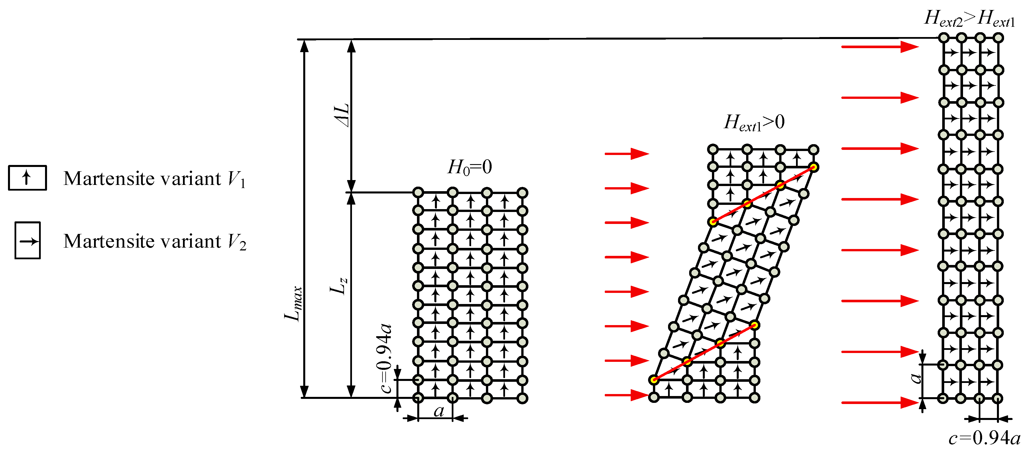
2.1. Basics of MSMA—Reorientation of a Crystal Lattice
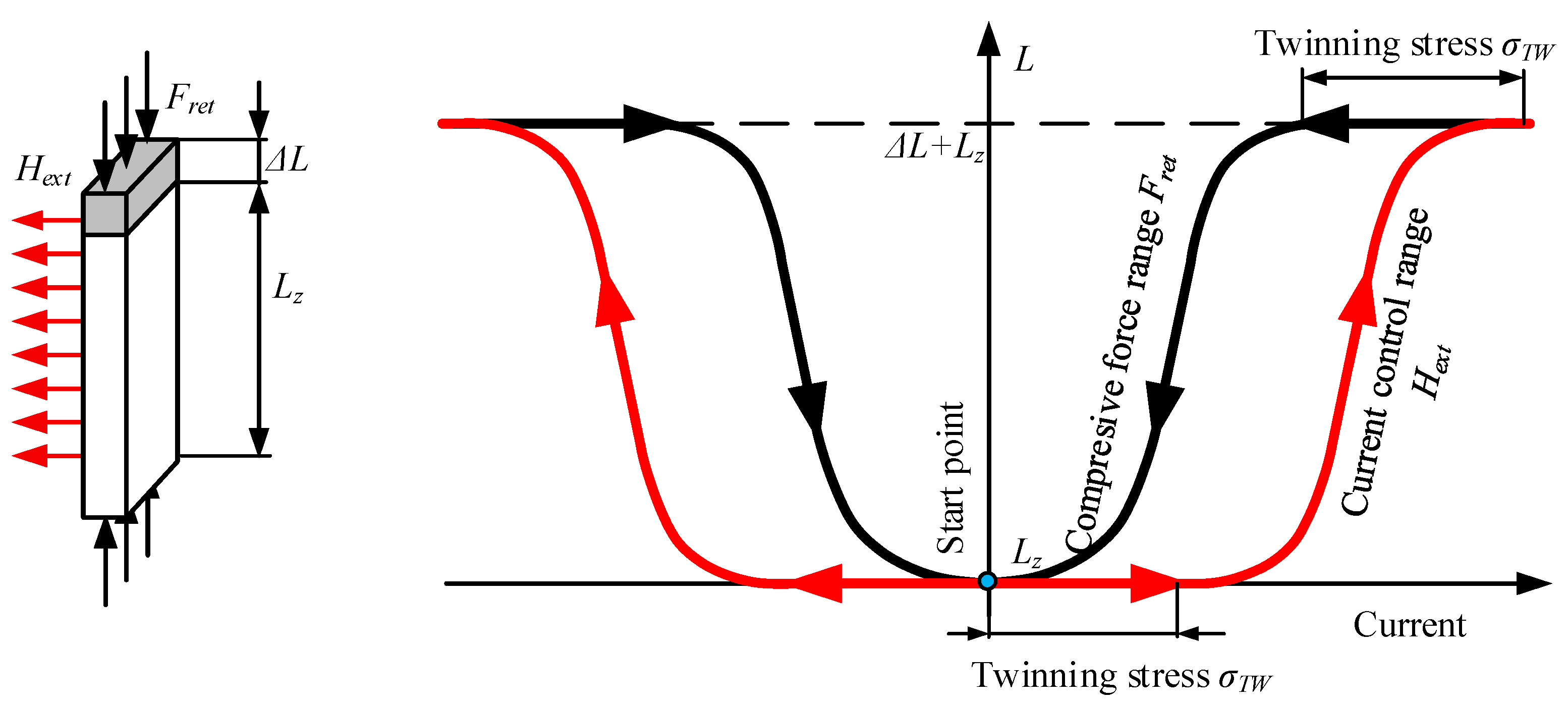
2.2. MSMA Actuator Design Survey

| Actuator Design | MSMA [mm3] | Excitation Current [A] | Strain [µm] | Actuator Design | MSMA [mm3] | Excitation Current [A] | Strain [µm] |
|---|---|---|---|---|---|---|---|
| Spring-returned mode | Push—push/push—pull mode | ||||||
| [29] | 2 × 5 × 20 | 2,2 | 200 | [26] | 2 × 3 × 10 | 5 | 150 |
| [21,26] | 1 × 2.5 × 20 | 5 | 400 | [32] | 3 × 5 × 20 | 2 | 1000 |
| [35] | 2 × 3 × 15 | 2 | 1000 | [40] | 3 × 5 × 20 | 2.5 | 260 |
| [41] | 1 × 2.5 × 20 | 5 | 400 | [31] | 3 × 5 × 15 | 3.5 | 280 |
| [42] | 1 × 2.5 × 20 | 1.4 | 900 | ||||
| [27] | 1 × 2.5 × 20 | 1.2 | 350 | ||||
| Mass placed above actuator | Compressive solenoid | ||||||
| [32,43] | 3 × 5 × 20 | 1 | 1000 | [34] | 1 × 2.5 × 20 | 2 | 450 |
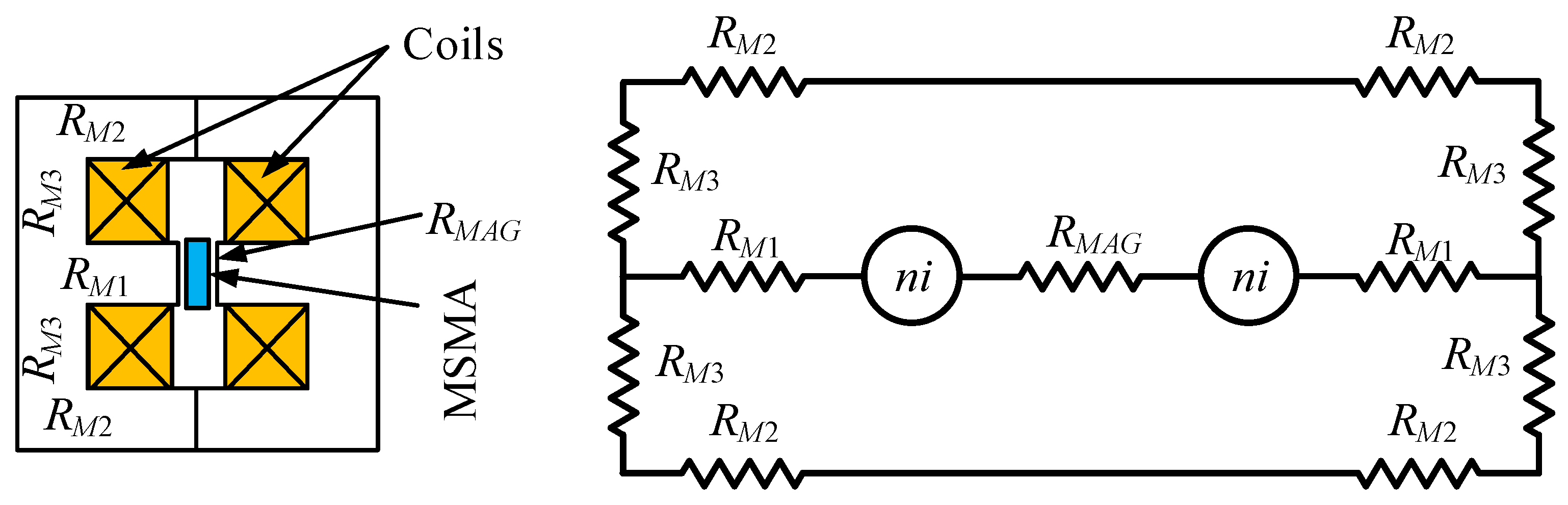
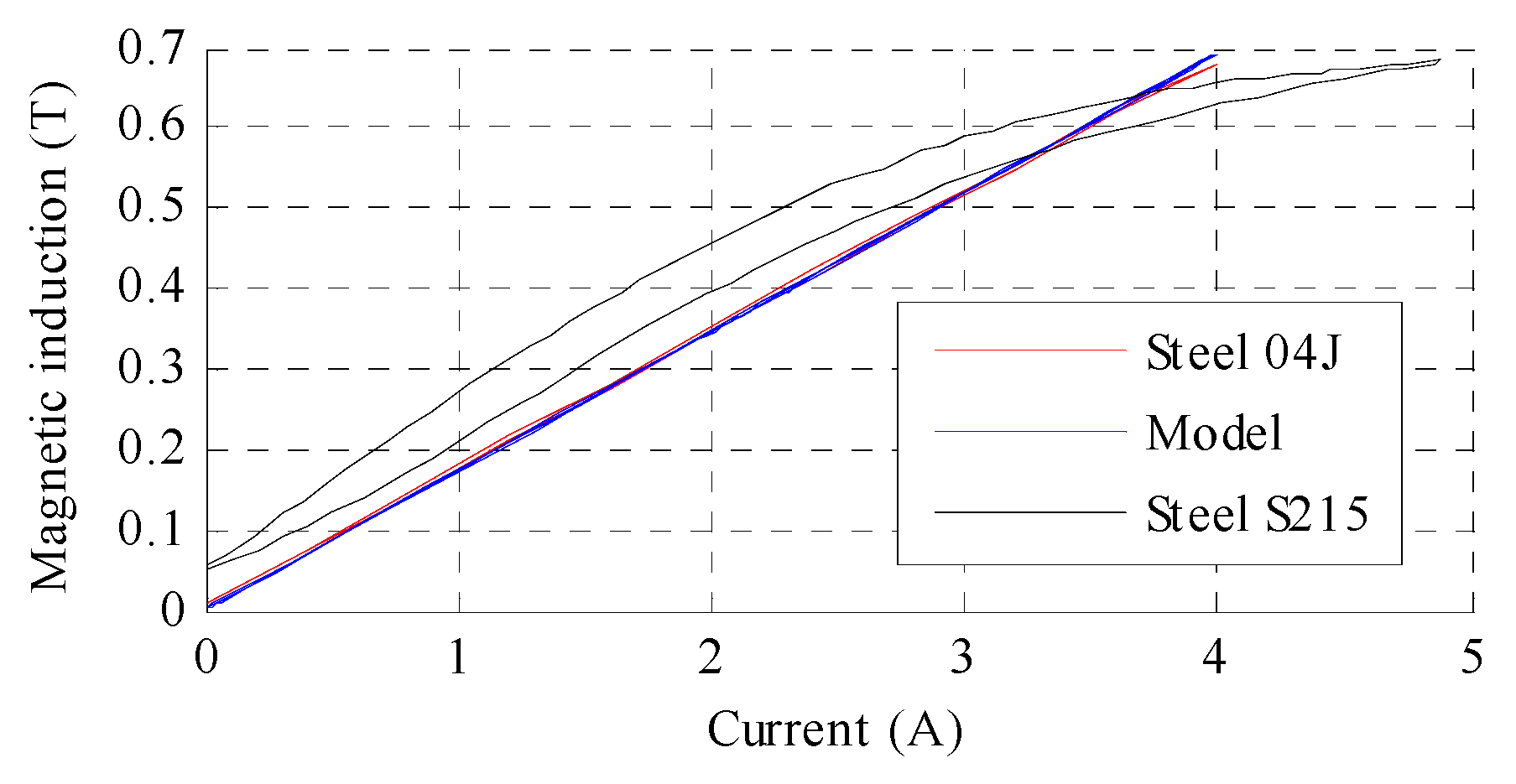
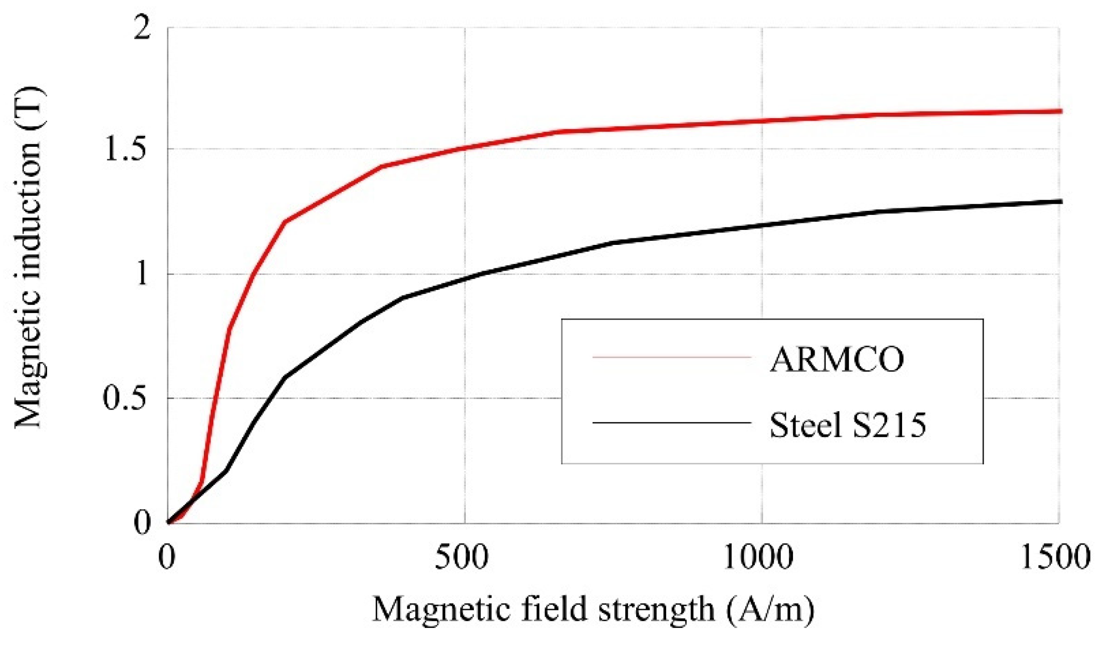
3. Basics of the MSMA Actuator Design Process
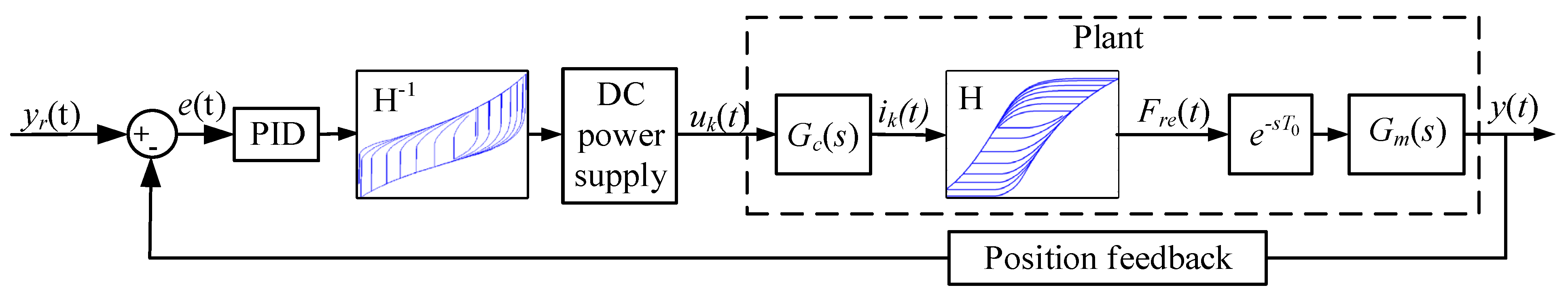
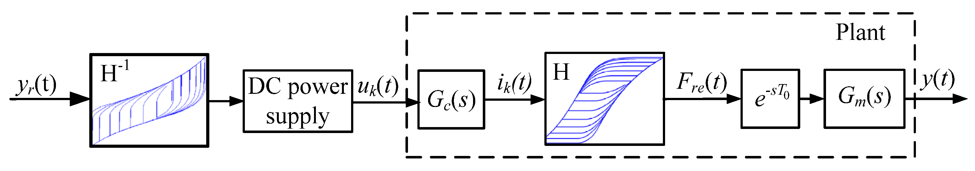
4. Modelling and Control of MSMA Actuator
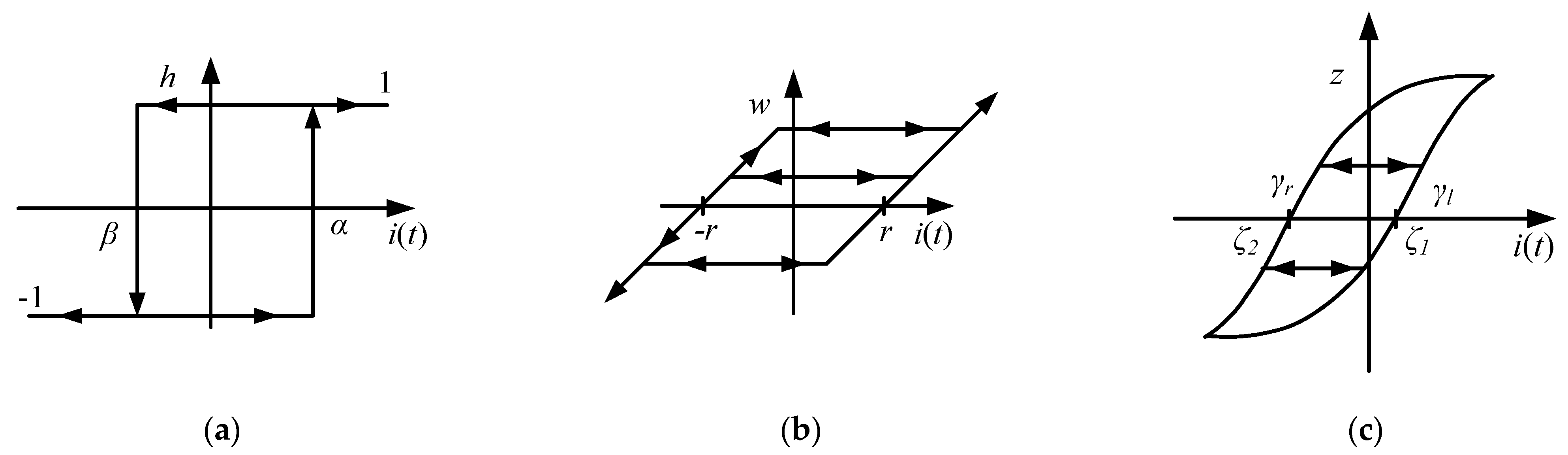
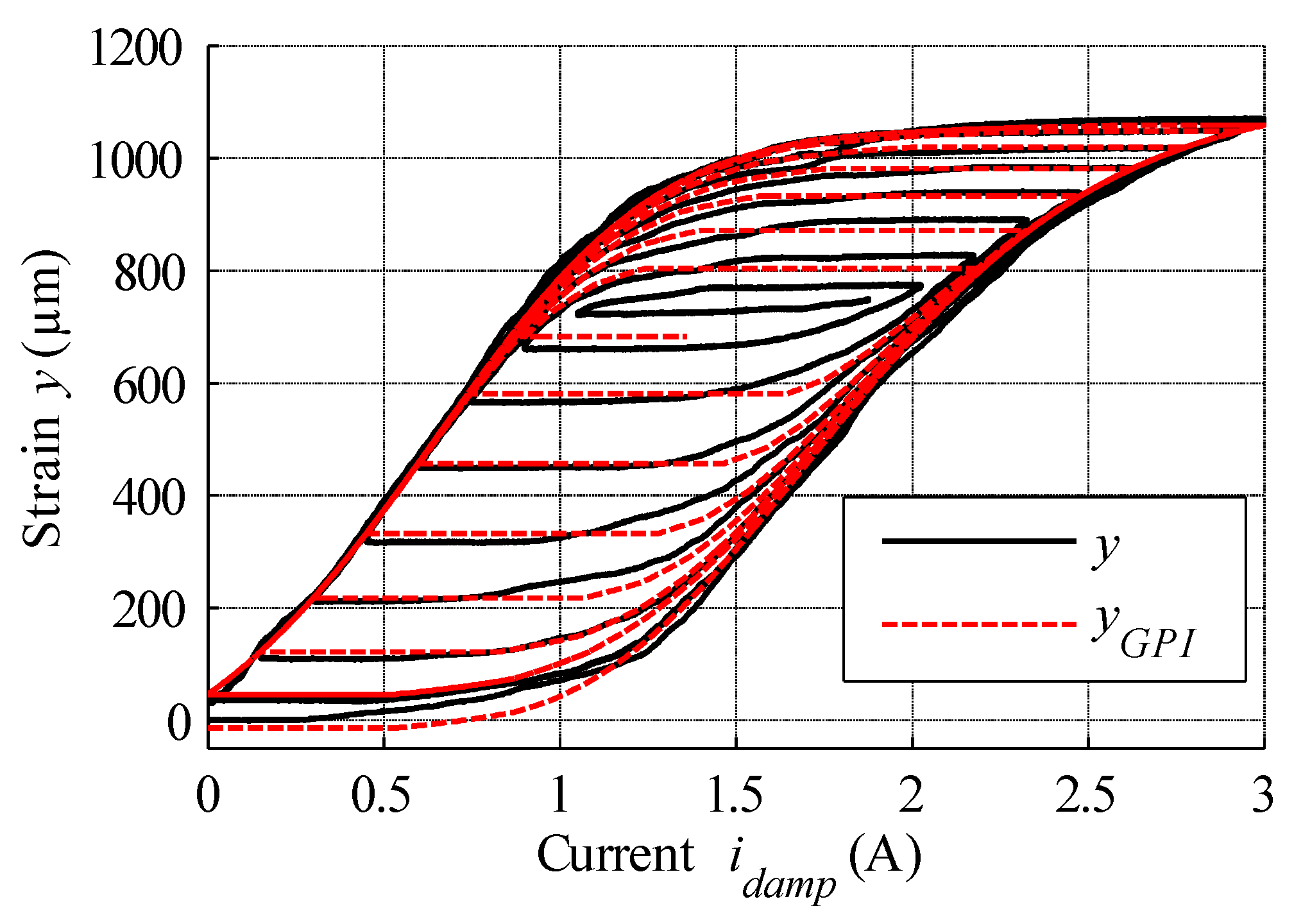
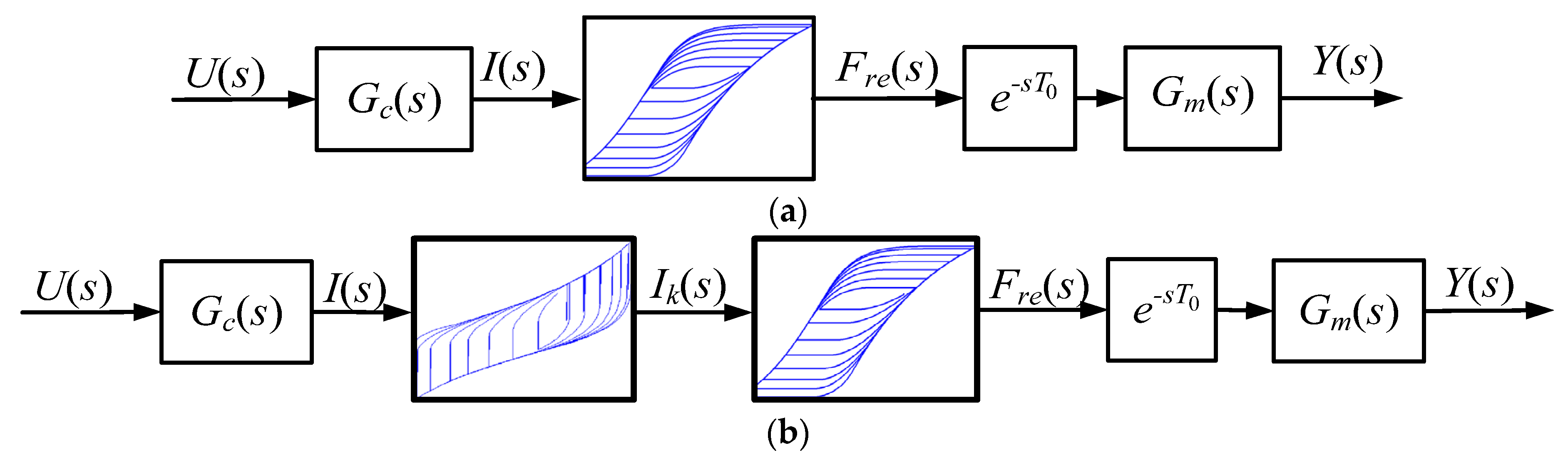
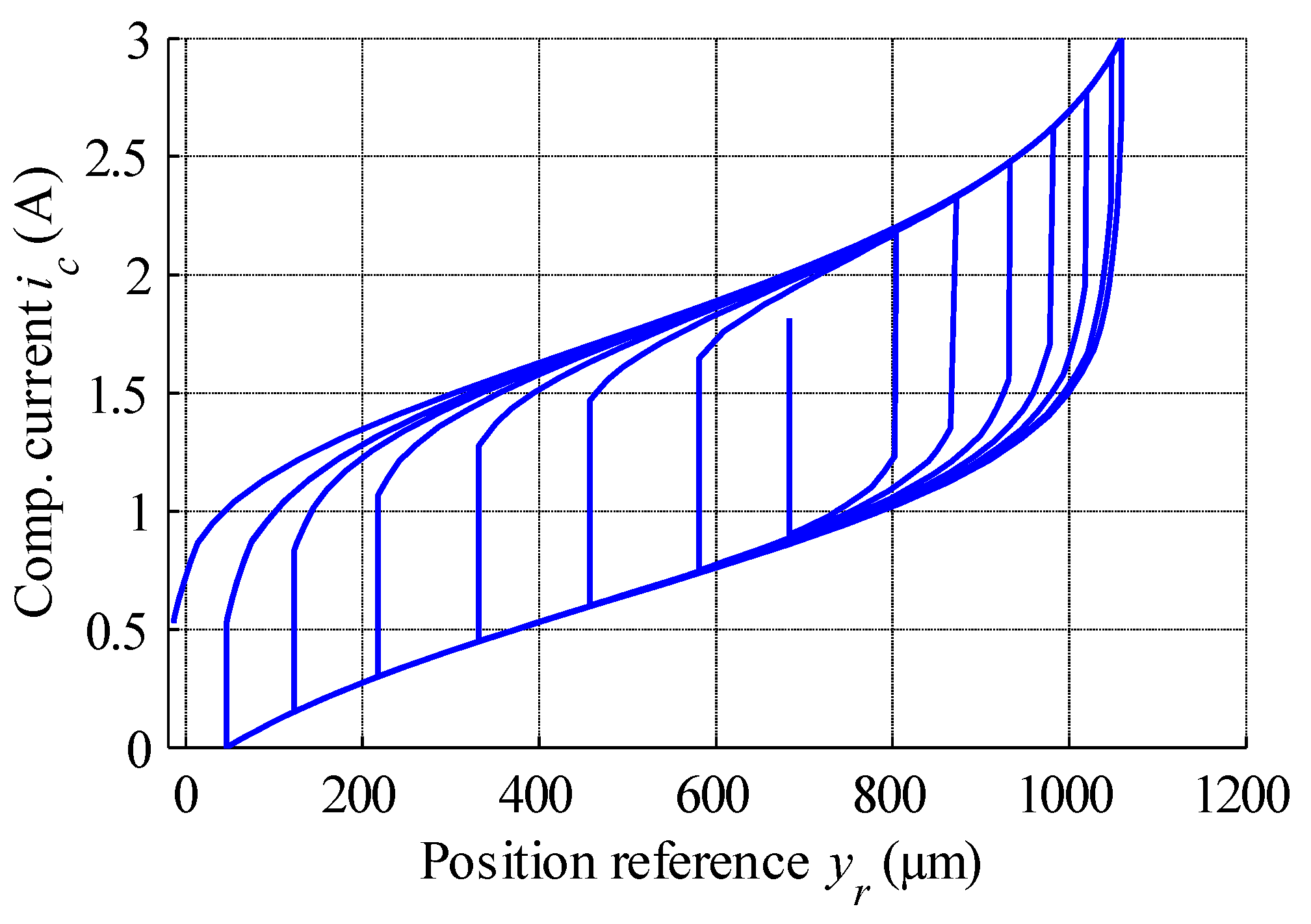
4.1. Static Characteristics Modelling via the Generalised Prandtl-Ishlinskii Model
4.2. Inverse of Generalised Prandtl-Ishlinskii Model
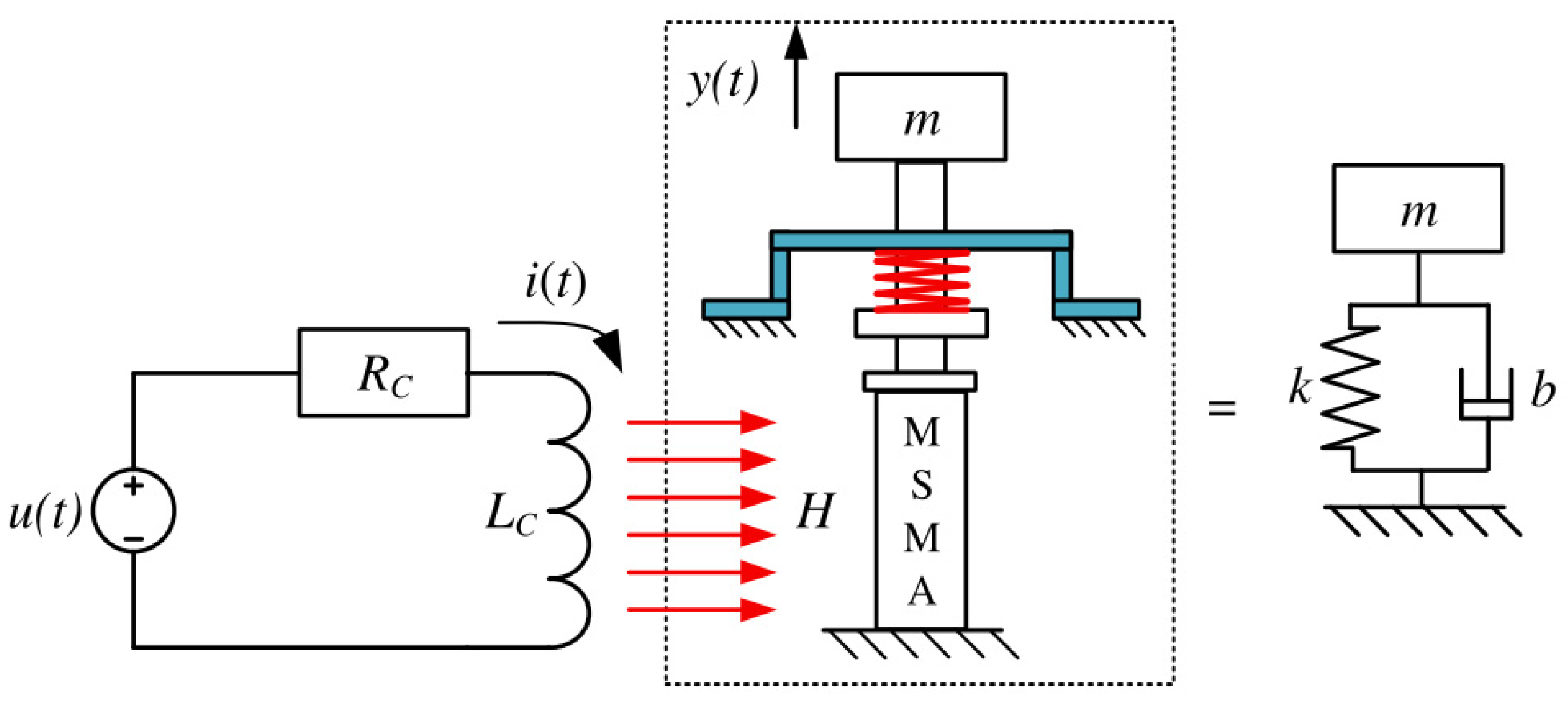
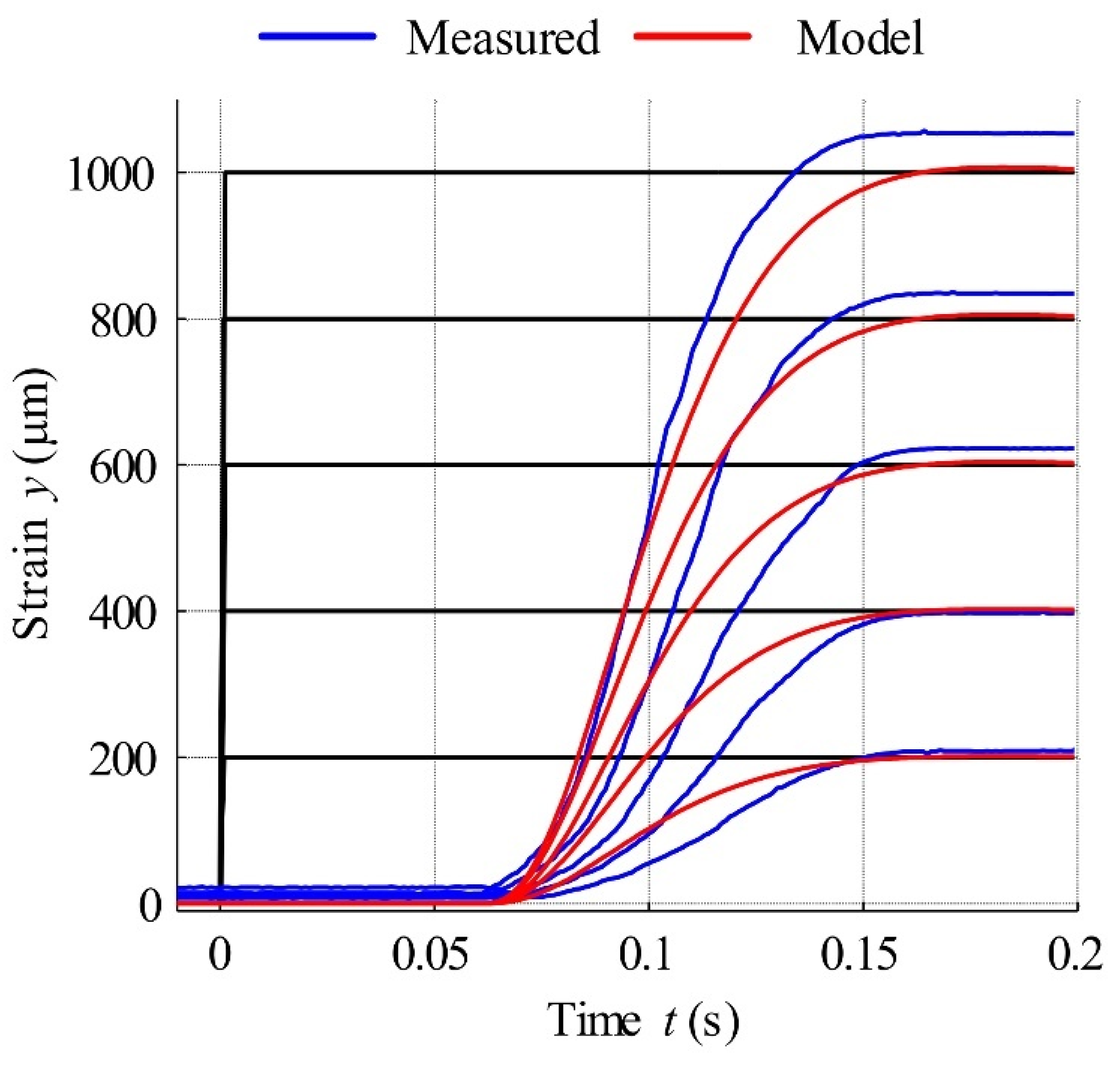
4.3. Actuator Dynamics Model
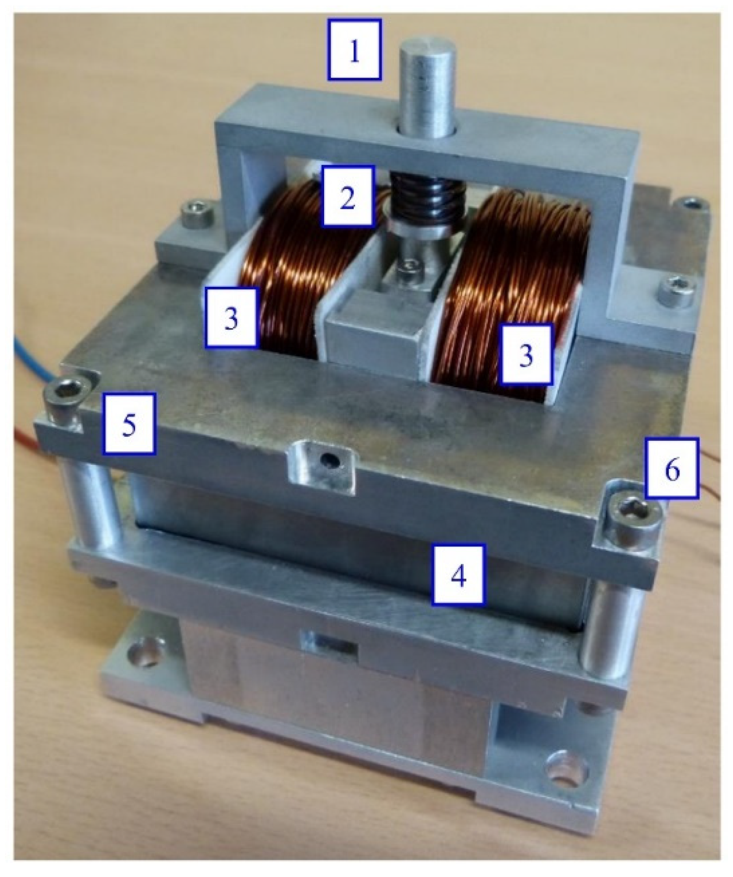
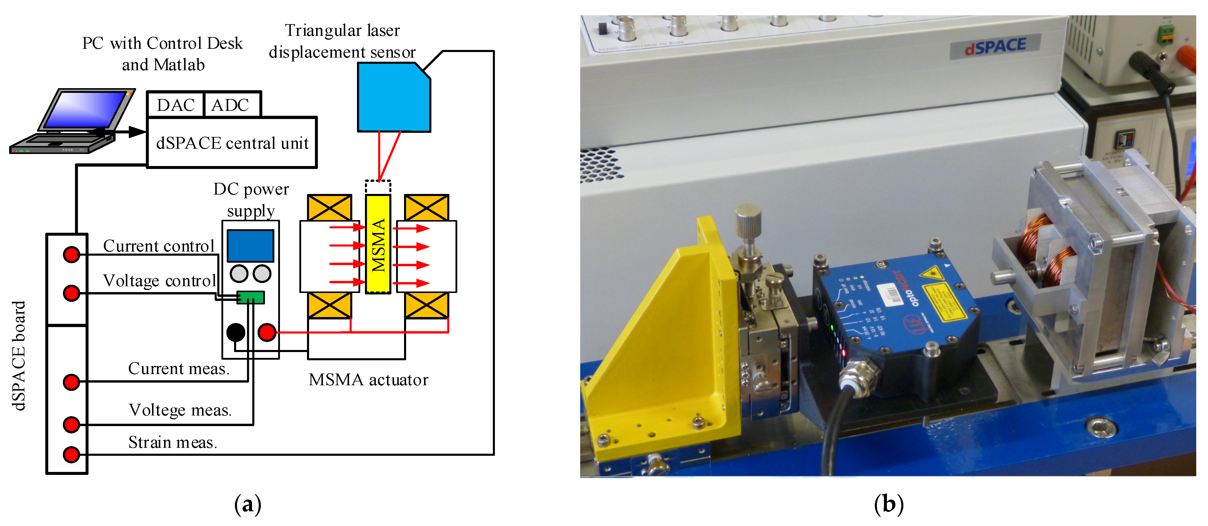
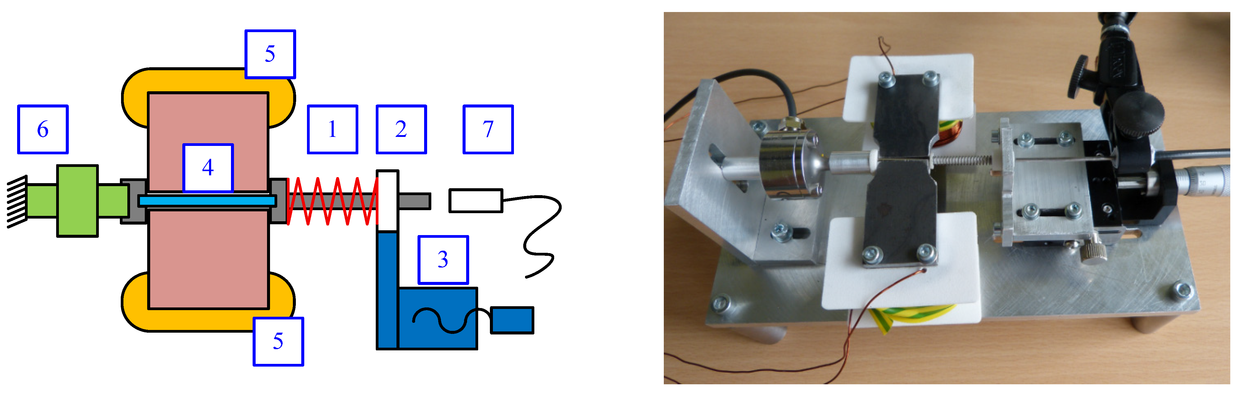
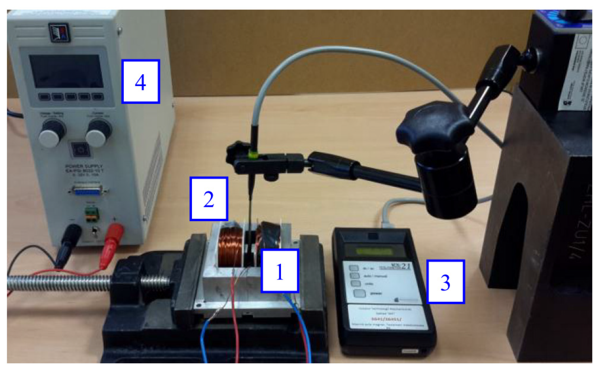
5. Test Stand
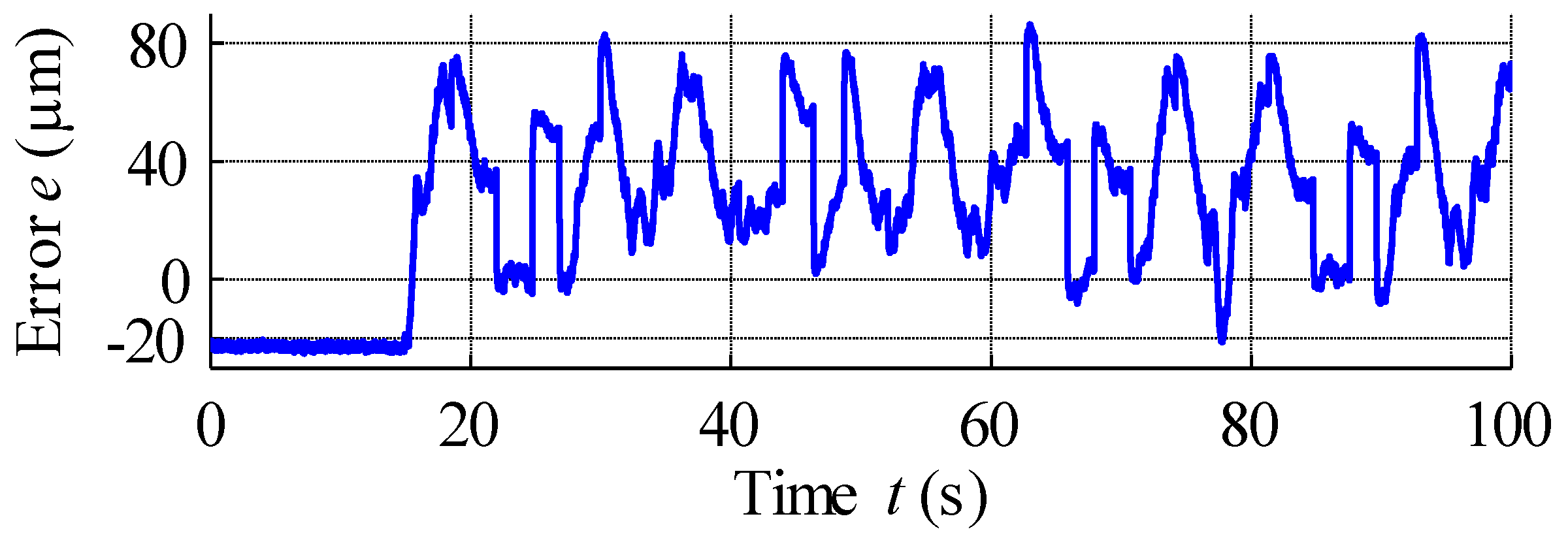
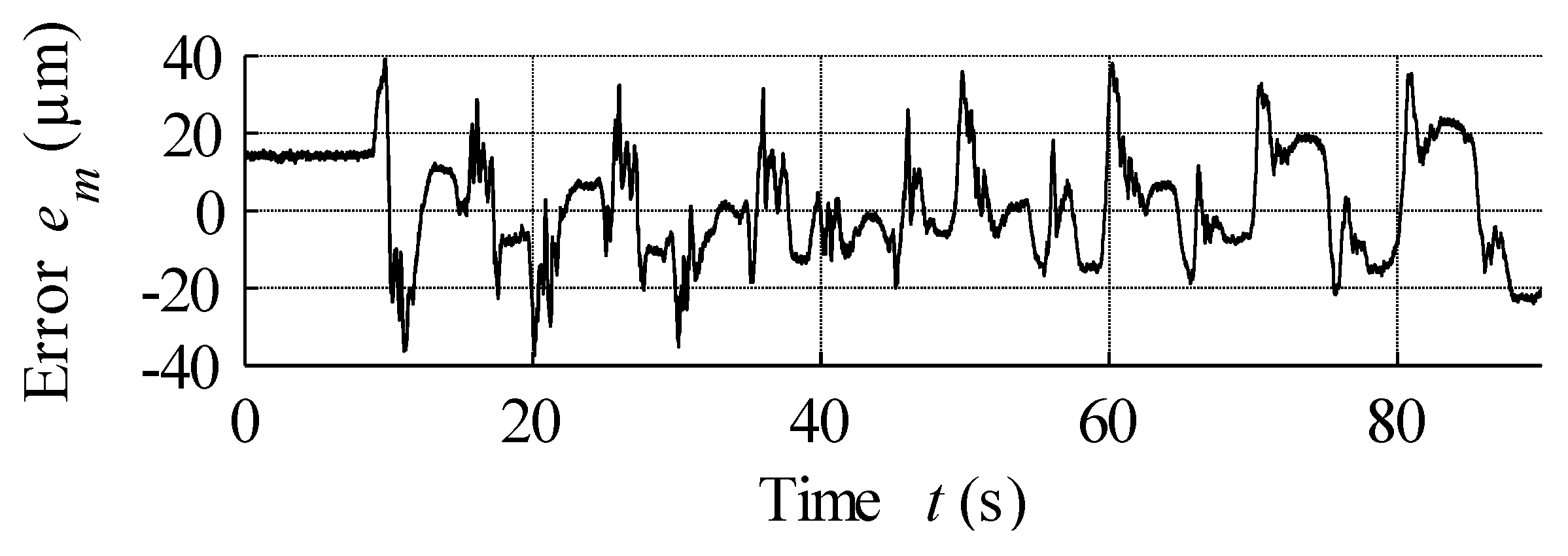
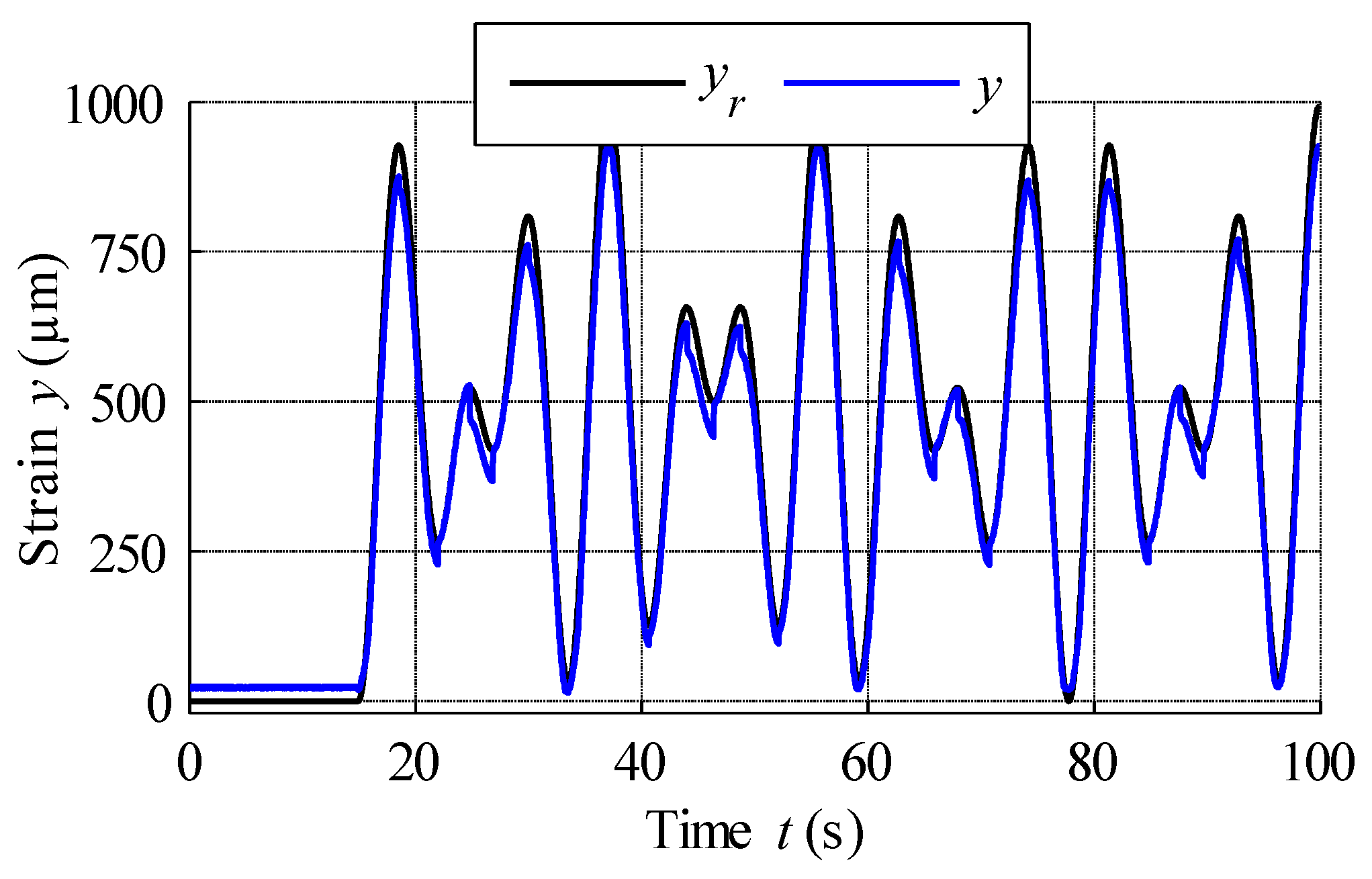
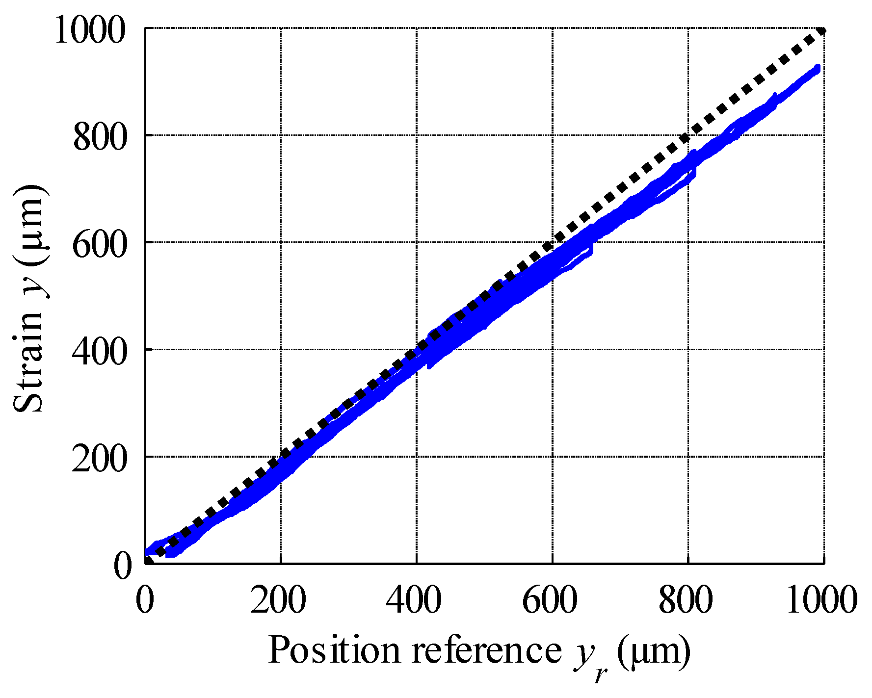
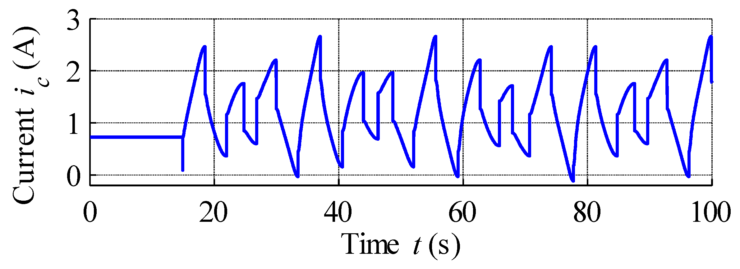
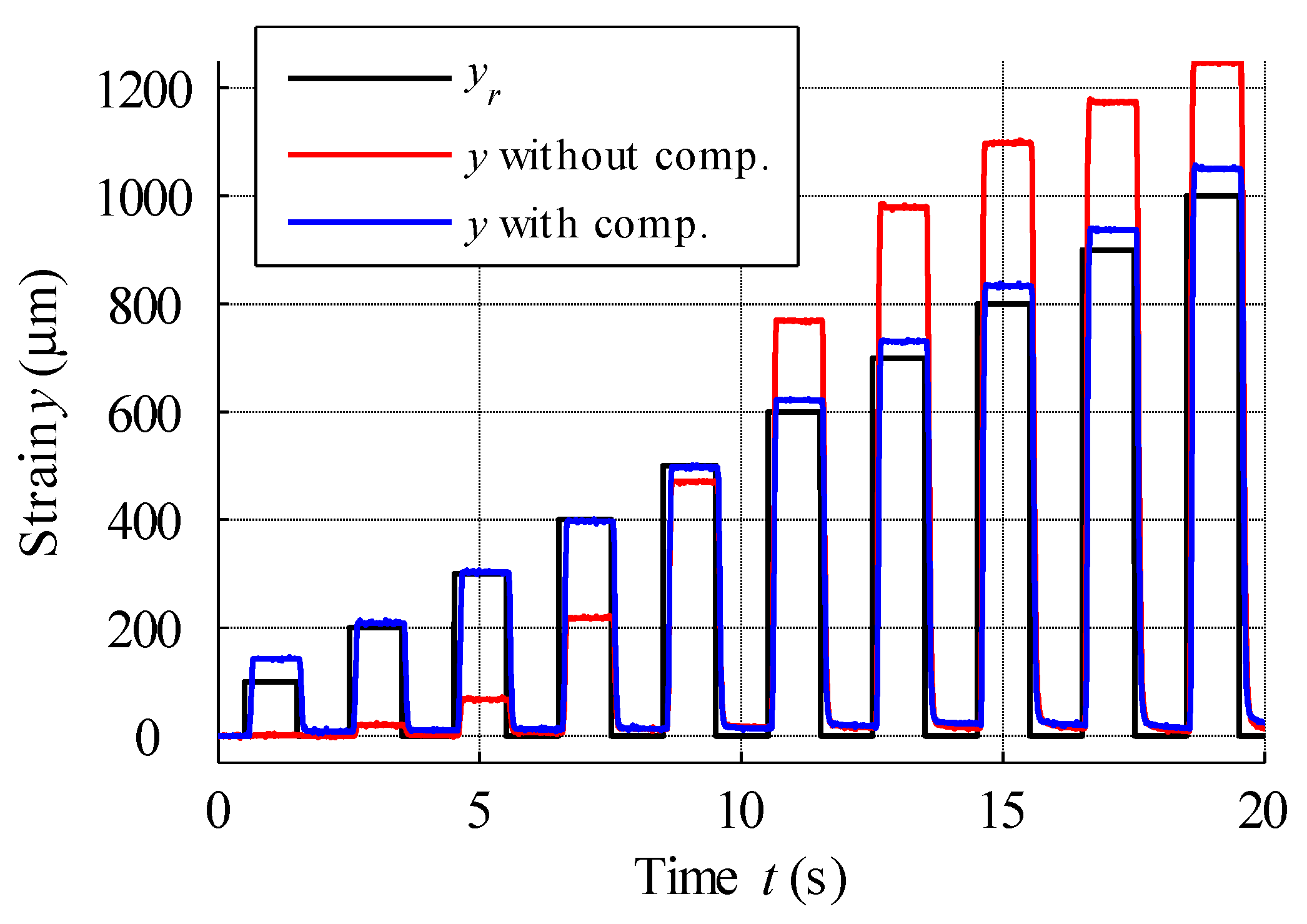
6. Hysteresis Compensation and MSMA Actuator Control
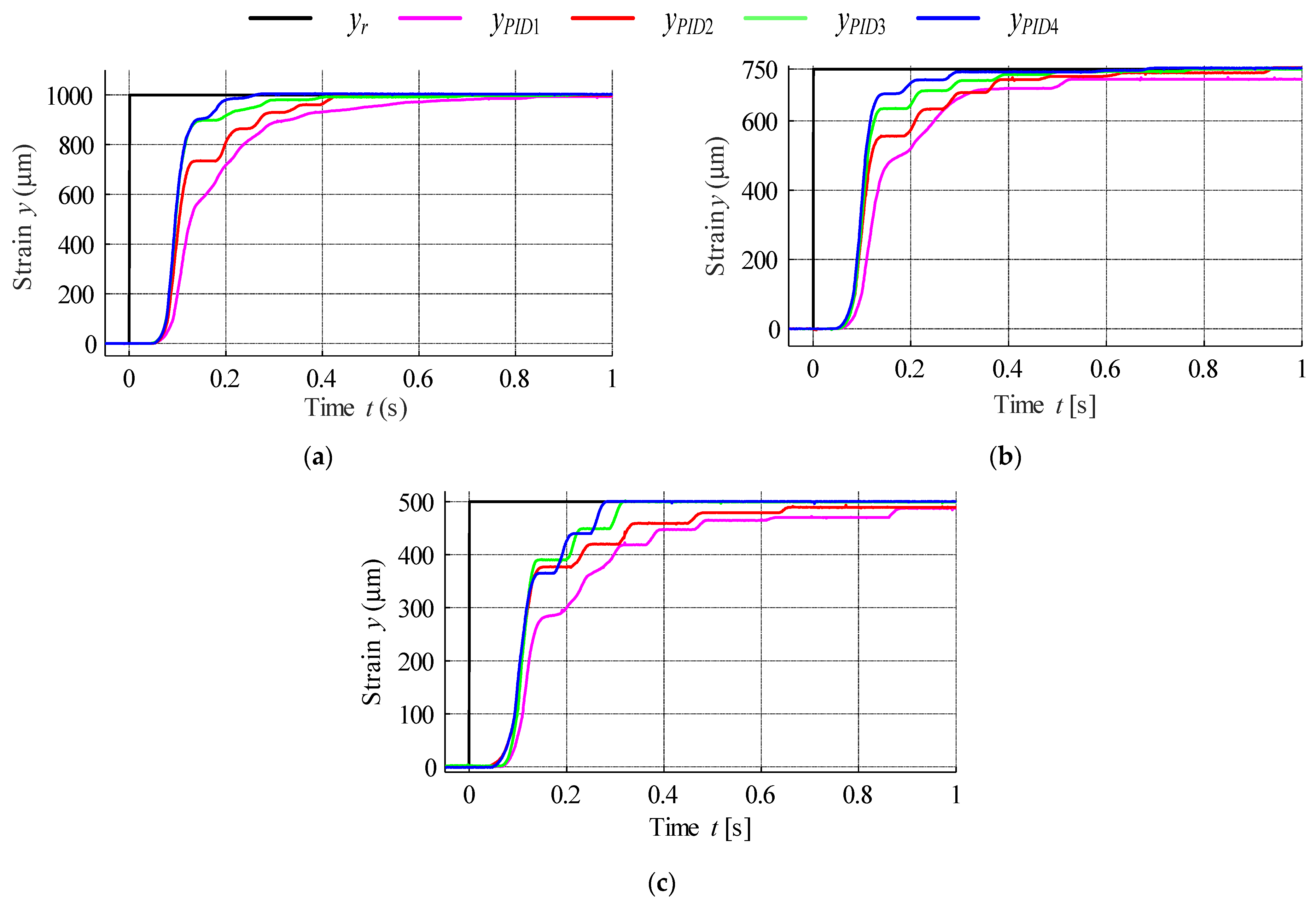
PID Control
7. Conclusions
Author Contributions
Funding
Institutional Review Board Statement
Informed Consent Statement
Data Availability Statement
Conflicts of Interest
References
- Higuchi, T. Next generation actuators leading breakthroughs. J. Mech. Sci. Technol. 2010, 24, 13–18. [Google Scholar] [CrossRef]
- Mohd Jani, J.; Leary, M.; Subic, A.; Gibson, M.A. A review of shape memory alloy research, applications and opportunities. Mater. Des. 2014, 56, 1078–1113. [Google Scholar] [CrossRef]
- Janocha, H. Adaptronics and Smart Structures; Springer: Berlin/Heidelberg, Germany, 2007. [Google Scholar]
- Schiepp, T.; Maier, M.; Pagounis, E.; Schluter, A.; Laufenberg, M. FEM-Simulation of Magnetic Shape Memory Actuators. IEEE Trans. Magn. 2014, 50, 989–992. [Google Scholar] [CrossRef]
- Habibullah, H.; Pota, H.R.; Petersen, I.R.; Rana, M.S. Tracking of triangular reference signals using LQG controllers for lateral positioning of an AFM scanner stage. IEEE/ASME Trans. Mechatron. 2014, 19, 1105–1114. [Google Scholar] [CrossRef]
- Karunanidhi, S.; Singaperumal, M. Design, analysis and simulation of magnetostrictive actuator and its application to high dynamic servo valve. Sens. Actuators A Phys. 2010, 157, 185–197. [Google Scholar] [CrossRef]
- Sangiah, D.K.; Plummer, A.R.; Bowen, C.R.; Guerrier, P. A novel piezohydraulic aerospace servovalve. Part 1: Design and modelling. Proc. Inst. Mech. Eng. Part J. Syst. Control Eng. 2013, 227, 371–389. [Google Scholar] [CrossRef]
- Sędziak, D. Basic investigations of electrohydraulic servovalve with piezo-bender element. Arch. Technol. Masz. Autom. 2006, 26, 185–190. [Google Scholar]
- Sędziak, D.; Regulski, R. Design and Investigations into the Piezobender Controlled Servovalve. In Solid State Phenomena; Trans Tech Publications Ltd.: Freienbach, Switzerland, 2015; Volume 220, pp. 520–525. [Google Scholar]
- Minase, J.; Lu, T.-F.; Cazzolato, B.; Grainger, S. A review, supported by experimental results, of voltage, charge and capacitor insertion method for driving piezoelectric actuators. Precis. Eng. 2010, 34, 692–700. [Google Scholar] [CrossRef]
- Liu, Y.-T.; Higuchi, T.; Fung, R.-F. A novel precision positioning table utilizing impact force of spring-mounted piezoelectric actuator—part I: Experimental design and results. Precis. Eng. 2003, 27, 14–21. [Google Scholar] [CrossRef]
- Zakerzadeh, M.R.; Sayyaadi, H. Precise position control of shape memory alloy actuator using inverse hysteresis model and model reference adaptive control system. Mechatronics 2013, 23, 1150–1162. [Google Scholar] [CrossRef]
- Williams, E.A.; Shaw, G.; Elahinia, M. Control of an automotive shape memory alloy mirror actuator. Mechatronics 2010, 20, 527–534. [Google Scholar] [CrossRef]
- Tiboni, M.; Borboni, A.; Mor, M.; Pomi, D. An innovative pneumatic mini-valve actuated by SMA Ni-Ti wires design and analysis. Proc. Inst. Mech. Eng. Part J. Syst. Control Eng. 2011, 225, 443–451. [Google Scholar] [CrossRef]
- Zakerzadeh, M.R.; Sayyaadi, H. Deflection Control of SMA-actuated Beam-like Structures in Nonlinear Large Deformation Mode. Am. J. Comput. Appl. Math. 2014, 4, 167–185. [Google Scholar]
- Sayyaadi, H.; Zakerzadeh, M.R. Position control of shape memory alloy actuator based on the generalized Prandtl–Ishlinskii inverse model. Mechatronics 2012, 22, 945–957. [Google Scholar] [CrossRef]
- Ullakko, K.; Huang, J.K.; Kantner, C.; O’Handley, R.C.; Kokorin, V.V. Large magnetic-field-induced strains in Ni2MnGa single crystals. Appl. Phys. Lett. 1996, 69, 1966–1968. [Google Scholar] [CrossRef]
- Ullakko, K. Magnetically controlled shape memory alloys: A new class of actuator materials. J. Mater. Eng. Perform. 1996, 5, 405–409. [Google Scholar] [CrossRef]
- Jokinen, T.; Ullakko, K.; Suorsa, I. Magnetic Shape Memory materials-new possibilities to create force and movement by magnetic fields. In Proceedings of the Fifth International Conference on Electrical Machines and Systems, Shenyang, China, 18–20 August 2001; Volume 1, pp. 20–23. [Google Scholar]
- Anon Materiały informacyjne ETO Magnetic. Available online: https://www.etogruppe.com/unternehmen/magnetoshape-r.html (accessed on 10 April 2022).
- Schlüter, K.; Riccardi, L.; Raatz, A. An Open-Loop Control Approach for Magnetic Shape Memory Actuators Considering Temperature Variations. Adv. Sci. Technol. 2013, 78, 119–124. [Google Scholar]
- Lin, C.-J.; Lin, C.-R.; Yu, S.-K.; Chen, C.-T. Hysteresis modeling and tracking control for a dual pneumatic artificial muscle system using Prandtl–Ishlinskii model. Mechatronics 2015, 28, 35–45. [Google Scholar] [CrossRef]
- Al Janaideh, M.; Rakheja, S.; Su, C.-Y. An analytical generalized Prandtl–Ishlinskii model inversion for hysteresis compensation in micropositioning control. IEEE/ASME Trans. Mechatron. 2011, 16, 734–744. [Google Scholar] [CrossRef]
- Flaga, S.; Sioma, A. Characteristics of Experimental MSMA-Based Pneumatic Valves. In Proceedings of the ASME 2013 Conference on Smart Materials, Adaptive Structures and Intelligent Systems, Snowbird, UT, USA, 16–18 September 2013; American Society of Mechanical Engineers: New York, NY, USA, 2013; p. V001T04A016. [Google Scholar]
- Holz, B.; Riccardi, L.; Janocha, H.; Naso, D. MSM actuators: Design rules and control strategies. Adv. Eng. Mater. 2012, 14, 668–681. [Google Scholar] [CrossRef]
- Schlüter, K.; Holz, B.; Raatz, A. Principle design of actuators driven by magnetic shape memory alloys. Adv. Eng. Mater. 2012, 14, 682–686. [Google Scholar] [CrossRef]
- Matsunaga, K.; Niguchi, N.; Hirata, K. Study on Starting Performance of Ni-Mn-Ga Magnetic Shape Memory Alloy Linear Actuator. IEEE Trans. Magn. 2013, 49, 2225–2228. [Google Scholar] [CrossRef]
- Gauthier, J.-Y.; Hubert, A.; Abadie, J.; Chaillet, N.; Lexcellent, C. Nonlinear Hamiltonian modelling of magnetic shape memory alloy based actuators. Sens. Actuators Phys. 2008, 141, 536–547. [Google Scholar] [CrossRef] [Green Version]
- Riccardi, L.; Naso, D.; Janocha, H.; Turchiano, B. A precise positioning actuator based on feedback-controlled magnetic shape memory alloys. Mechatronics 2012, 22, 568–576. [Google Scholar] [CrossRef]
- Tellinen, J.; Suorsa, I.; Jääskeläinen, A.; Aaltio, I.; Ullakko, K. Basic properties of magnetic shape memory actuators. In Proceedings of the 8th International Conference ACTUATOR, Bremen, Germany, 10–12 June 2002; pp. 566–569. [Google Scholar]
- Riccardi, L.; Holz, B.; Janocha, H. Exploiting hysteresis in position control: The magnetic shape memory push-push actuator. In Proceedings of the Innovative Small Drives and Micro-Motor Systems, Nuremberg, Germany, 19–20 September 2013; pp. 1–6. [Google Scholar]
- Hubert, A.; Calchand, N.; Le Gorrec, Y.; Gauthier, J.-Y. Magnetic Shape Memory Alloys as smart materials for micro-positioning devices. Adv. Electromagn. 2012, 1, 75–84. [Google Scholar] [CrossRef] [Green Version]
- Wegener, K.; Blumenthal, P.; Raatz, A. Development of a miniaturized clamping device driven by magnetic shape memory alloys. J. Intell. Mater. Syst. Struct. 2014, 25, 1062–1068. [Google Scholar] [CrossRef]
- Le Gall, Y.; Bolzmacher, C. Design and characterization of a multi-stable magnetic shape memory alloy hybrid actuator. Microsyst. Technol. 2014, 20, 533–543. [Google Scholar] [CrossRef]
- Schiepp, T.; Pagounis, E.; Laufenberg, M. Magnetic Shape Memory Actuators for Fluidic Applications. In Proceedings of the 9th International Fluid Power Conference, Aachen, Germany, 24–26 March 2014. [Google Scholar]
- Janocha, H. Magnetic Field Driven Unconventional Actuators. In Proceedings of the Adaptronic Congress, Berlin, Germany, 20–21 May 2008. [Google Scholar]
- Suorsa, I.; Tellinen, J.; Pagounis, E.; Aaltio, I.; Ullakko, K. Applications of magnetic shape memory actuators. In Proceedings of the 8th International Conference ACTUATOR, Bremen, Germany, 10–12 June 2002; pp. 158–161. [Google Scholar]
- Niskanen, A.J. Magnetic Shape Memory (MSM) Alloys for Energy Harvesting and Sensing Applications. In Proceedings of the WoWSS 2012, Aalto University 2nd Workshop on Wireless Sensor Systems, Espoo, Finland, 11 December 2012. [Google Scholar]
- Majewska, K.; Zak, A.; Ostachowicz, W. Magnetic Shape Memory (MSM) actuators in practical use. J. Phys. Conf. Ser. 2009, 181, 012073. [Google Scholar] [CrossRef]
- Riccardi, L.; Rosmarino, M.; Naso, D.; Janocha, H. Positioning system with a magnetic shape memory push-push actuator. In Proceedings of the 13th International Conference on New Actuators ACTUATOR12, Bremen, Germany, 18–20 June 2012. [Google Scholar]
- Flaga, S.; Oprzędkiewicz, I.; Sapiński, B. Characteristics of an experimental MSMA-based actuator. Solid State Phenom. 2013, 198, 283–288. [Google Scholar] [CrossRef]
- Adaptamat conference presentations. Available online: http://www.adaptamat.com/publications/ (accessed on 21 April 2015).
- Gauthier, J.-Y.; Hubert, A.; Abadie, J.; Chaillet, N.; Lexcellent, C. Original hybrid control for robotic structures using magnetic shape memory alloys actuators. In Proceedings of the 2007 IEEE/RSJ International Conference on Intelligent Robots and Systems, San Diego, CA, USA, 29 October–2 November 2007; pp. 747–752. [Google Scholar]
- Suorsa, I.; Tellinen, J.; Aaltio, I.; Pagounis, E.; Ullakko, K. Design of active element for msm-actuator. In Proceedings of the ACTUATOR 2004/9th International Conference on New Actuators, Bremen, Germany, 14–16 June 2004. [Google Scholar]
- Anon Smalley Steel Ring Company. Available online: https://www.smalley.com/ (accessed on 10 April 2020).
- Minorowicz, B.; Nowak, A. Force generation survey in magnetic shape memory alloys. Arch. Mech. Technol. Autom. 2013, 33, 37–46. [Google Scholar]
- Visintin, A. Differential Models of Hysteresis; Springer: New York, NY, USA, 1994. [Google Scholar]
- Jiles, D.C.; Atherton, D.L. Theory of ferromagnetic hysteresis. J. Magn. Magn. Mater. 1986, 61, 48–60. [Google Scholar] [CrossRef]
- Kuhnen, K.; Krejci, P. Compensation of complex hysteresis and creep effects in piezoelectrically actuated systems—A new Preisach modeling approach. IEEE Trans. Autom. Control. 2009, 54, 537–550. [Google Scholar] [CrossRef]
- Krasnosel’skiǐ, M.A.; Pokrovskiǐ, A.V. Systems with Hysteresis; Springer: Berlin/Heidelberg, Germany, 1989. [Google Scholar]
- Al Janaideh, M.; Mao, J.; Rakheja, S.; Xie, W.; Su, C.-Y. Generalized Prandtl-Ishlinskii hysteresis model: Hysteresis modeling and its inverse for compensation in smart actuators. In Proceedings of the 2008 47th IEEE Conference on Decision and Control, Cancun, Mexico, 9–11 December 2008. [Google Scholar]
- Mayergoyz, I.D. Mathematical Model of Hysteresis; Springer: New York, NY, USA, 1991. [Google Scholar]
- Al Janaideh, M.; Rakheja, S.; Su, C. A generalized Prandtl-Ishlinskii model for characterizing the hysteresis and saturation nonlinearities of smart actuators. Smart Mater. Struct. 2009, 18, 045001. [Google Scholar] [CrossRef]
- Macki, J.W.; Nistri, P.; Zecca, P. Mathematical models for hysteresis. SIAM Rev. 1993, 35, 94–123. [Google Scholar] [CrossRef] [Green Version]
- Hassani, V.; Tjahjowidodo, T.; Do, T.N. A survey on hysteresis modeling, identification and control. Mech. Syst. Signal Processing 2014, 49, 209–233. [Google Scholar] [CrossRef]
- Liu, Y.; Shan, J.; Meng, Y.; Zhu, D. Modeling and identification of asymmetric hysteresis in smart actuators: A modified MS model approach. IEEE/ASME Trans. Mechatron. 2015, 21, 38–43. [Google Scholar]
- Lin, C.-J.; Lin, P.-T. Tracking control of a biaxial piezo-actuated positioning stage using generalized Duhem model. Comput. Math. Appl. 2012, 64, 766–787. [Google Scholar] [CrossRef] [Green Version]
- Su, C.-Y.; Stepanenko, Y.; Svoboda, J.; Leung, T.-P. Robust adaptive control of a class of nonlinear systems with unknown backlash-like hysteresis. IEEE Trans. Autom. Control 2000, 45, 2427–2432. [Google Scholar] [CrossRef] [Green Version]
- Bouc, R. Forced vibrations of mechanical systems with hysteresis. In Proceedings of the Fourth Conference on Nonlinear Oscillations, Prague, Czech Republic, 5–9 September 1967. [Google Scholar]
- Wen, Y.K. Method for random vibration of hysteretic systems. J. Eng. Mech. Div. 1976, 102, 249–263. [Google Scholar] [CrossRef]
- Yu, Y.; Zhang, C.; Zhou, M. NARMAX Model-Based Hysteresis Modeling of Magnetic Shape Memory Alloy Actuators. IEEE Trans. Nanotechnol. 2020, 19, 1–4. [Google Scholar] [CrossRef]
- Yu, Y.; Zhang, C.; Wang, Y.; Zhou, M. Neural-Network-Based Iterative Learning Control for Hysteresis in a Magnetic Shape Memory Alloy Actuator. IEEE/ASME Trans. Mechatron. 2022, 27, 928–939. [Google Scholar] [CrossRef]


| GPIM Parameters | ||
|---|---|---|
| Model order m | 10 | |
| Operator scope | 11 (0, 1…10) | |
| Envelope functions γ | a0 = 1.906 | b0 = 1.9931 |
| a1 = 1.1530 | b1 = 1.2839 | |
| a2= −1.9515 | b2= −0.8924 | |
| a3 = 1.5358 | b3 = 1.2934 | |
| Density function parameters p(r) | α = 0.1255 | |
| ρ = 110.5488 | ||
| τ = 2.9377 | ||
| Error Type/Error Value | (µm) | % |
|---|---|---|
| MSMA actuator strain | 1074.5 | 100 |
| Max. positive error | 39.73 | 3.70 |
| Max. negative error | −37.45 | 3.49 |
| Max. absolute error | 39.73 | 3.70 |
| Mean error | 2.58 | 0.24 |
| Mean absolute error | 11.71 | 1.09 |
| RMSE | 13.9 | 1.29 |
| Reference yr(t) | ||
|---|---|---|
| (µm) | % | |
| MSMA actuator strain | 1000 | 100 |
| Max. positive error | 86.37 | 8.64 |
| Max. negative error | −24.98 | 2.50 |
| Max. positive error + |Max. negative error| | 111.35 | 11.14 |
| Max. absolute error | 86.37 | 8.64 |
| Mean error | 26.25 | 2.63 |
| Mean absolute error | 33.75 | 3.38 |
| RMSE | 39.62 | 3.96 |
| Controller | Gains | ||
|---|---|---|---|
| kp | ki | kd | |
| PID1 | 0.3 | 6 | 0.01 |
| PID2 | 0.5 | 8 | 0.01 |
| PID3 | 0.55 | 10 | 0.015 |
| PID4 | 0.57 | 11,3 | 0.02 |
| Rise Time tu [ms] for yr ±5% | ||||||
|---|---|---|---|---|---|---|
| Controller | Position reference yr [µm] | |||||
| 500 | +25 | 750 | +37.5 | 1000 | +50 | |
| −25 | −37.5 | −50 | ||||
| PID1 | 770 | 510 | 480 | |||
| PID2 | 470 | 370 | 340 | |||
| PID3 | 301 | 295 | 250 | |||
| PID4 | 230 | 202 | 180 | |||
| Integral Absolute Error | |||
|---|---|---|---|
| Controller | Position reference yr [µm] | ||
| 500 | 750 | 1000 | |
| PID1 | 126.3 | 154.9 | 187.1 |
| PID2 | 92.4 | 126.3 | 142.8 |
| PID3 | 70.25 | 99.02 | 116.9 |
| PID4 | 72.35 | 89.44 | 108.4 |
Publisher’s Note: MDPI stays neutral with regard to jurisdictional claims in published maps and institutional affiliations. |
© 2022 by the authors. Licensee MDPI, Basel, Switzerland. This article is an open access article distributed under the terms and conditions of the Creative Commons Attribution (CC BY) license (https://creativecommons.org/licenses/by/4.0/).
Share and Cite
Minorowicz, B.; Milecki, A. Design and Control of Magnetic Shape Memory Alloy Actuators. Materials 2022, 15, 4400. https://doi.org/10.3390/ma15134400
Minorowicz B, Milecki A. Design and Control of Magnetic Shape Memory Alloy Actuators. Materials. 2022; 15(13):4400. https://doi.org/10.3390/ma15134400
Chicago/Turabian StyleMinorowicz, Bartosz, and Andrzej Milecki. 2022. "Design and Control of Magnetic Shape Memory Alloy Actuators" Materials 15, no. 13: 4400. https://doi.org/10.3390/ma15134400
APA StyleMinorowicz, B., & Milecki, A. (2022). Design and Control of Magnetic Shape Memory Alloy Actuators. Materials, 15(13), 4400. https://doi.org/10.3390/ma15134400