Author Contributions
Conceptualization, D.J.Y. and S.S.; methodology, D.J.Y., R.A. and S.S.; software, M.F.A.C.R.; validation, M.F.A.C.R.; formal analysis, M.F.A.C.R. and D.J.Y.; investigation, M.F.A.C.R., D.J.Y. and R.A.; resources, R.A. and Y.S.; data curation, M.F.A.C.R., D.J.Y., R.A. and Y.S.; writing—original draft preparation, M.F.A.C.R. and D.J.Y.; writing—-review and editing, Y.S. and S.S.; visualization, M.F.A.C.R.; supervision, D.J.Y., Y.S. and S.S.; project administration, D.J.Y. and S.S.; funding acquisition, D.J.Y. and S.S. All authors have read and agreed to the published version of the manuscript.
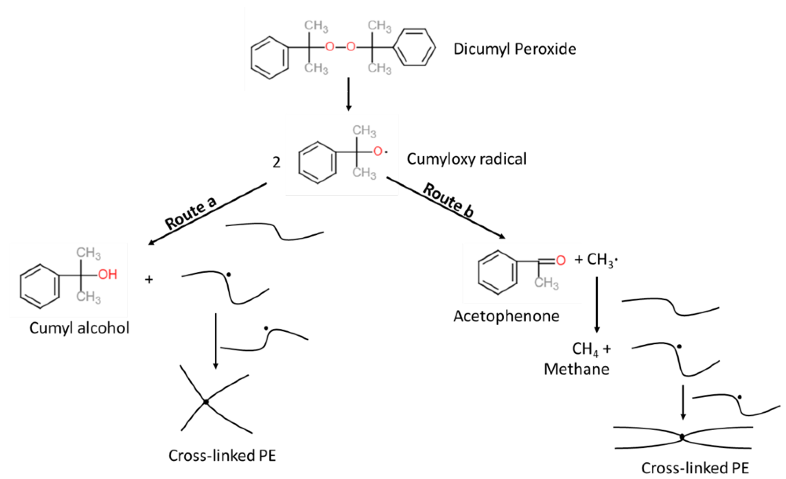
Figure 1.
Dicumyl peroxide (DCP)-initiated polyethylene (PE) cross-linking reaction scheme compiled from Andrews et al. [
1] and Sun et al. [
13].
Figure 1.
Dicumyl peroxide (DCP)-initiated polyethylene (PE) cross-linking reaction scheme compiled from Andrews et al. [
1] and Sun et al. [
13].
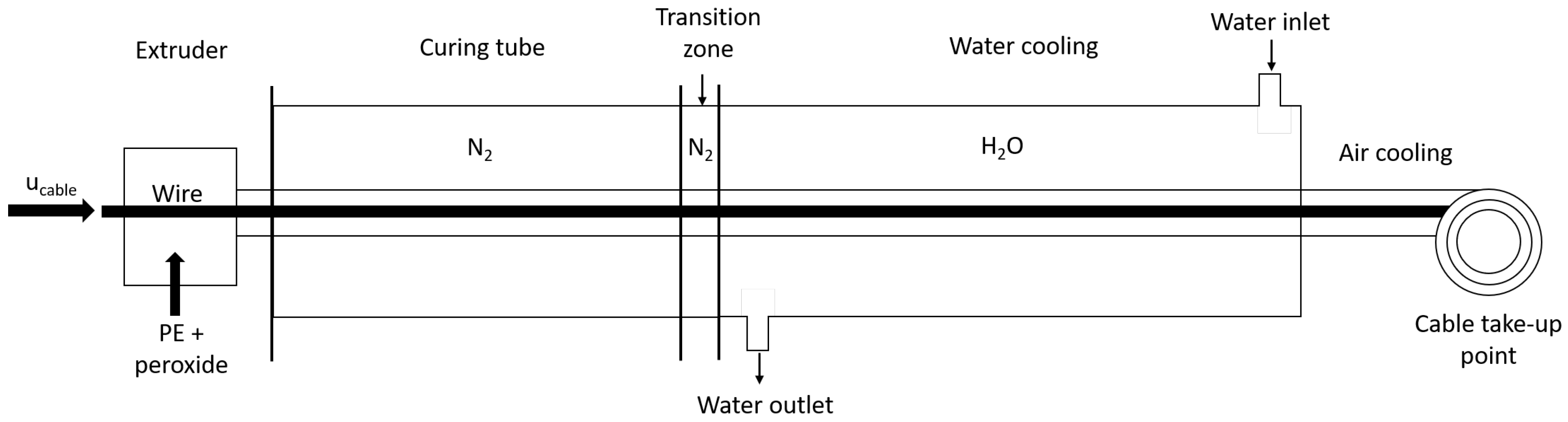
Figure 2.
Schematic of power cable production line.
Figure 2.
Schematic of power cable production line.
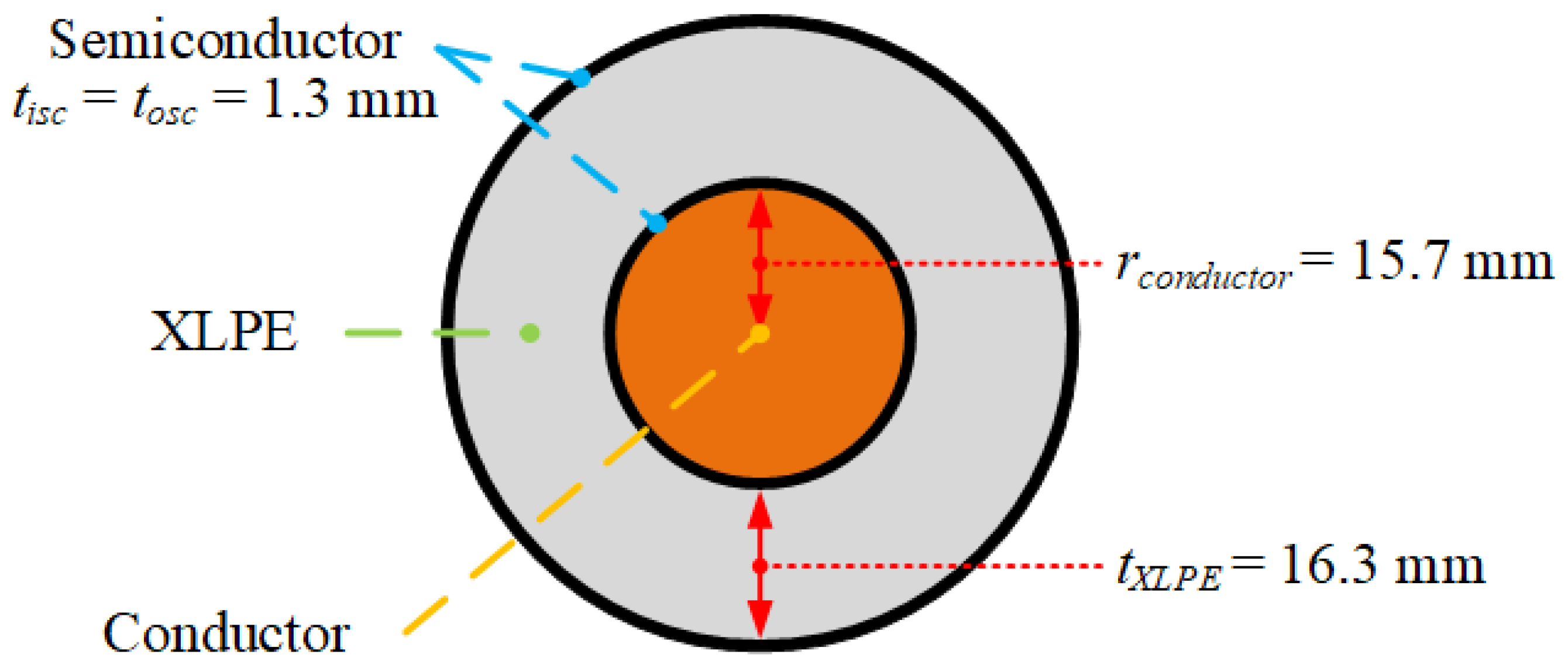
Figure 3.
The 132 kV cable specification.
Figure 3.
The 132 kV cable specification.
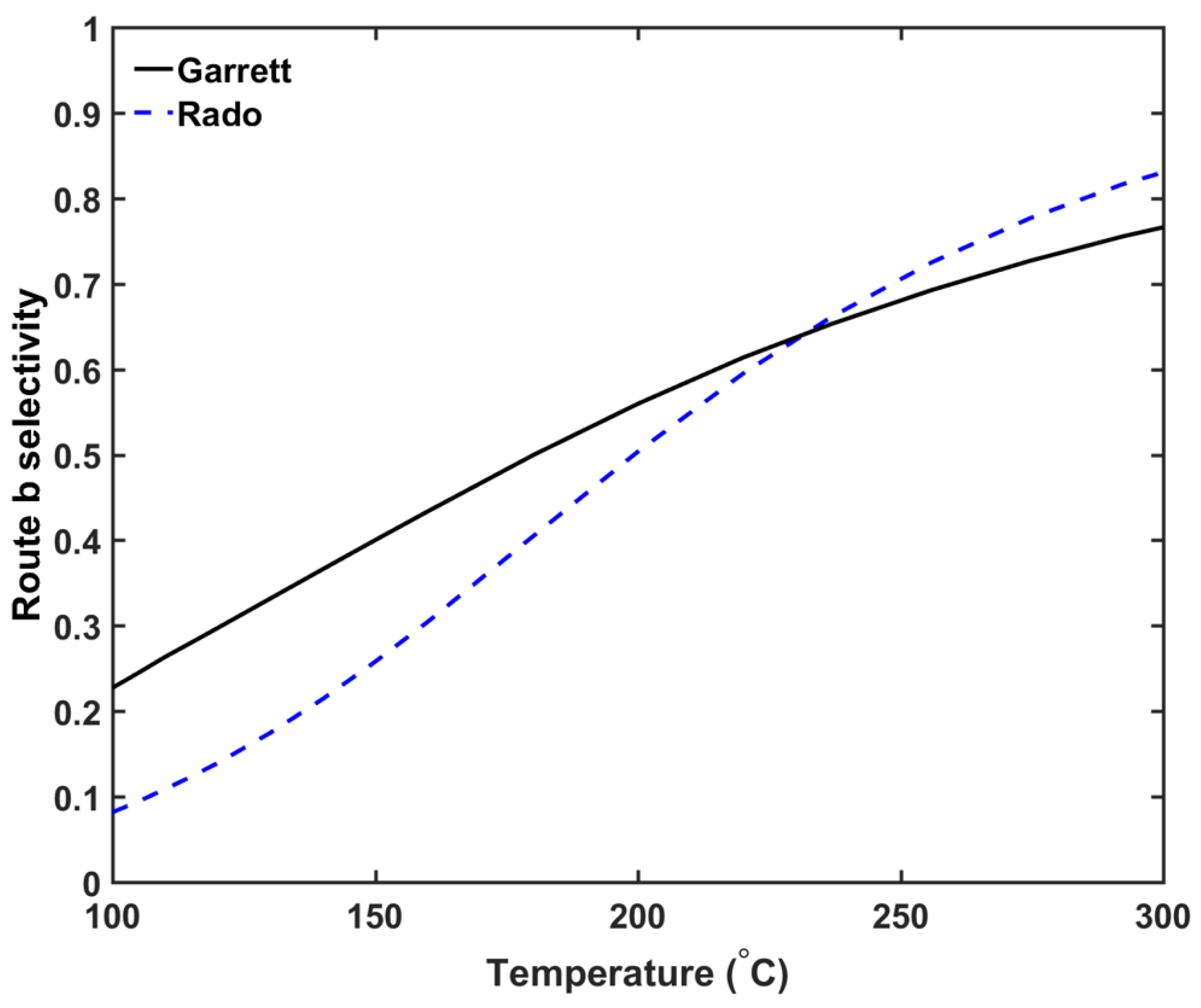
Figure 4.
Route
b reaction selectivity profile [
28,
29].
Figure 4.
Route
b reaction selectivity profile [
28,
29].
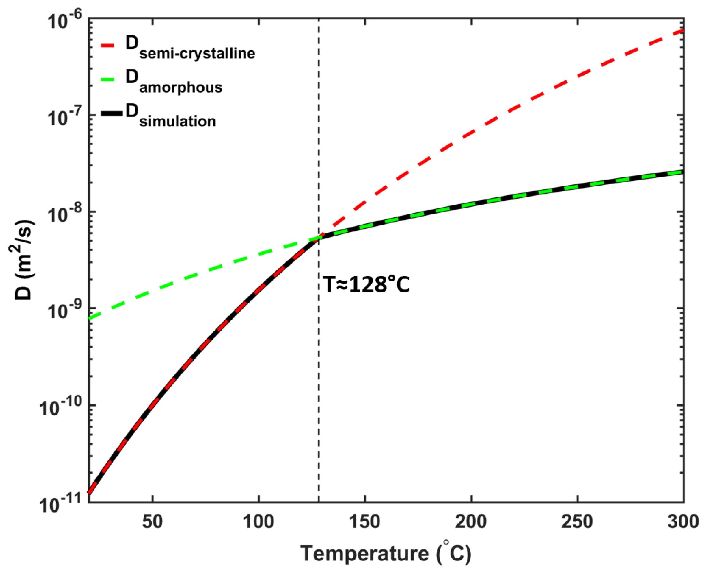
Figure 5.
CH
diffusion coefficient variations in XLPE as semi-crystalline [
13] (red line) and amorphous [
35] (green line) phases of the XLPE, which were then combined to represent the diffusion coefficient variation applied in the simulation (black line).
Figure 5.
CH
diffusion coefficient variations in XLPE as semi-crystalline [
13] (red line) and amorphous [
35] (green line) phases of the XLPE, which were then combined to represent the diffusion coefficient variation applied in the simulation (black line).
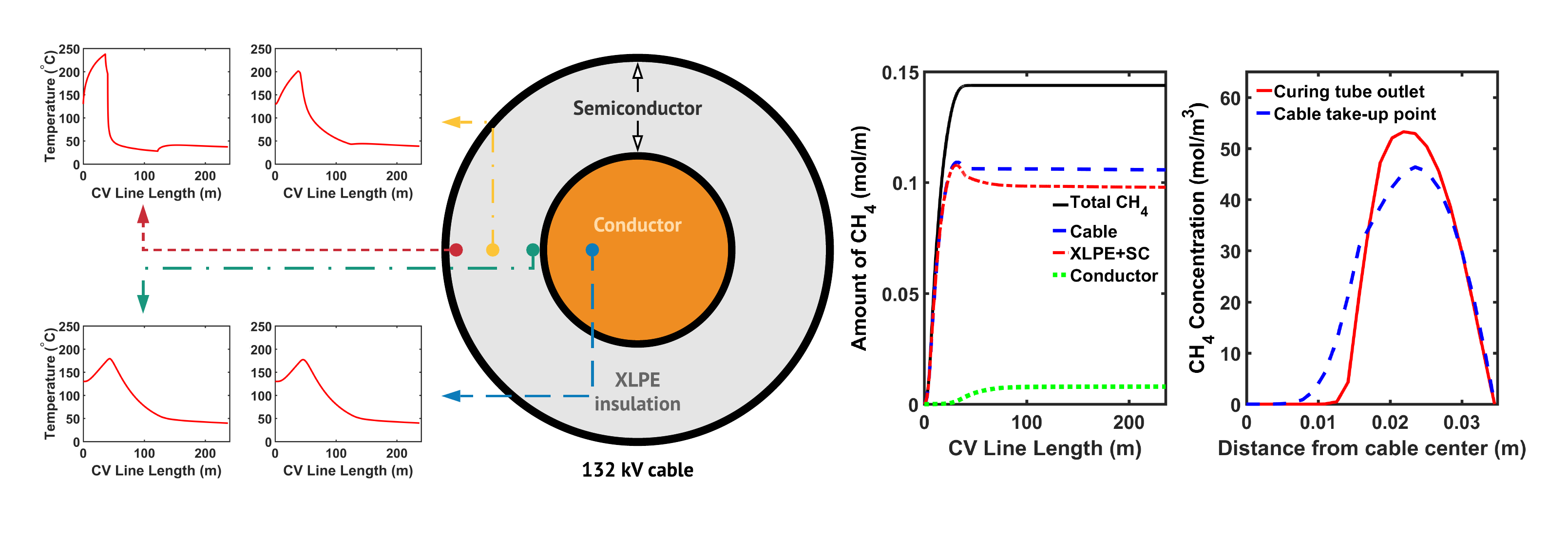
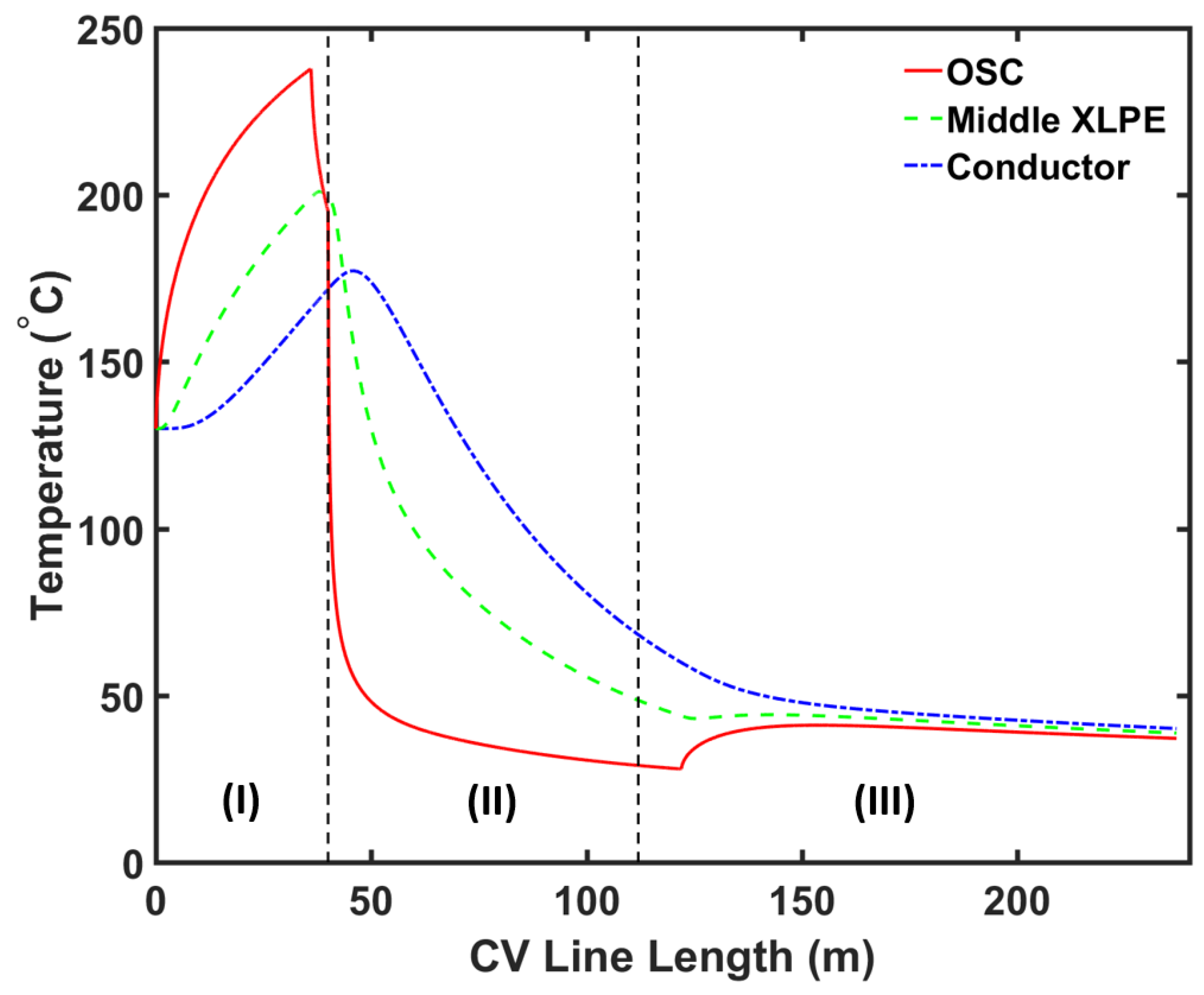
Figure 6.
CV line temperature profile at different distances from the cable centre. Segment (I), (II) and (III) correspond to the curing tube and transition zone, water-cooling, and air-cooling segments, respectively.
Figure 6.
CV line temperature profile at different distances from the cable centre. Segment (I), (II) and (III) correspond to the curing tube and transition zone, water-cooling, and air-cooling segments, respectively.
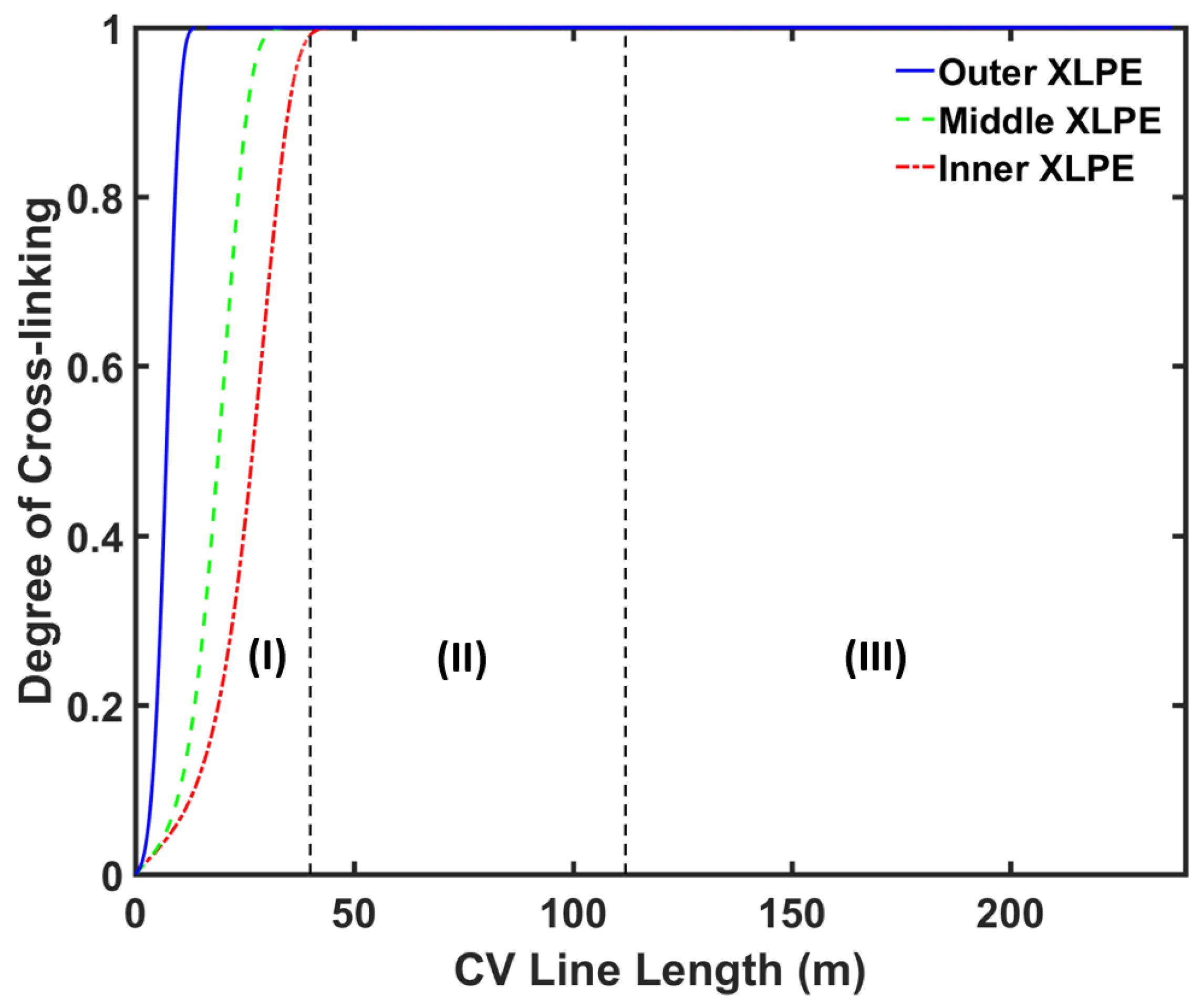
Figure 7.
CV line cross-linking profile at different distances from the cable centre. Segments (I), (II) and (III) correspond to the curing tube and transition zone, water-cooling, and air-cooling segments, respectively.
Figure 7.
CV line cross-linking profile at different distances from the cable centre. Segments (I), (II) and (III) correspond to the curing tube and transition zone, water-cooling, and air-cooling segments, respectively.
Figure 8.
Radial cross-linking profile at different distances from the CV line inlet.
Figure 8.
Radial cross-linking profile at different distances from the CV line inlet.
Figure 9.
Axial CH
4 concentration profile across the CV line, computed based on two different cross-linking reaction selectivity profiles. The reaction selectivity profile based on Rado’s data [
28] and Garrett’s data [
29] was used for computing the reaction selectivity in (
a,
b), respectively. Segments
(I), (II), and (III) correspond to the curing tube and transition zone, water-cooling, and air-cooling
segments, respectively.
Figure 10.
Radial CH4 concentration profile at (a) curing tube exit, (b) cable take-up point. segment (i) corresponds to conductor layer while segment (ii) corresponds to XLPE and SC layers.
Figure 10.
Radial CH4 concentration profile at (a) curing tube exit, (b) cable take-up point. segment (i) corresponds to conductor layer while segment (ii) corresponds to XLPE and SC layers.
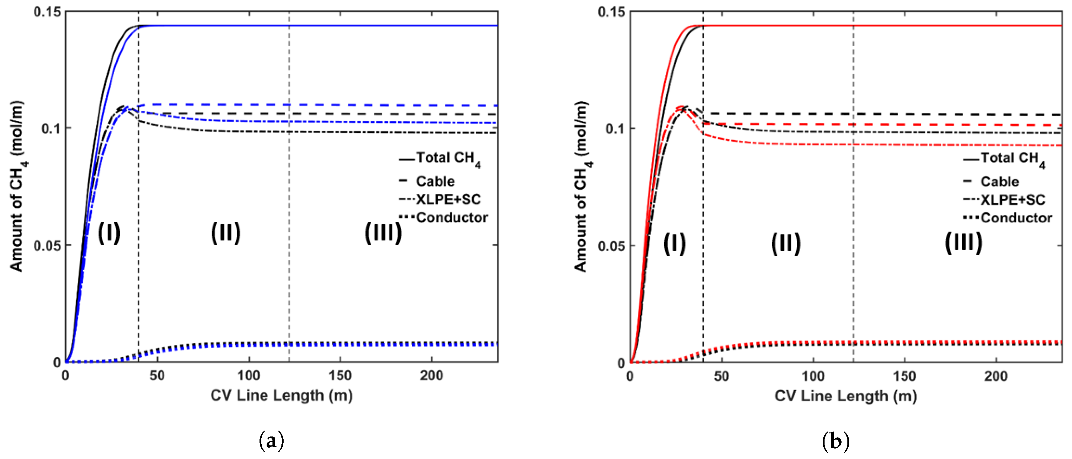
Figure 11.
Axial CH4 concentration profile across CV line for curing temperature study. The black line represents base case, blue line in (a) represents Case 1a, and red line in (b) represents Case 1b. Segment (I), (II) and (III) correspond to curing tube and transition zone, water cooling, and air cooling segments, respectively.
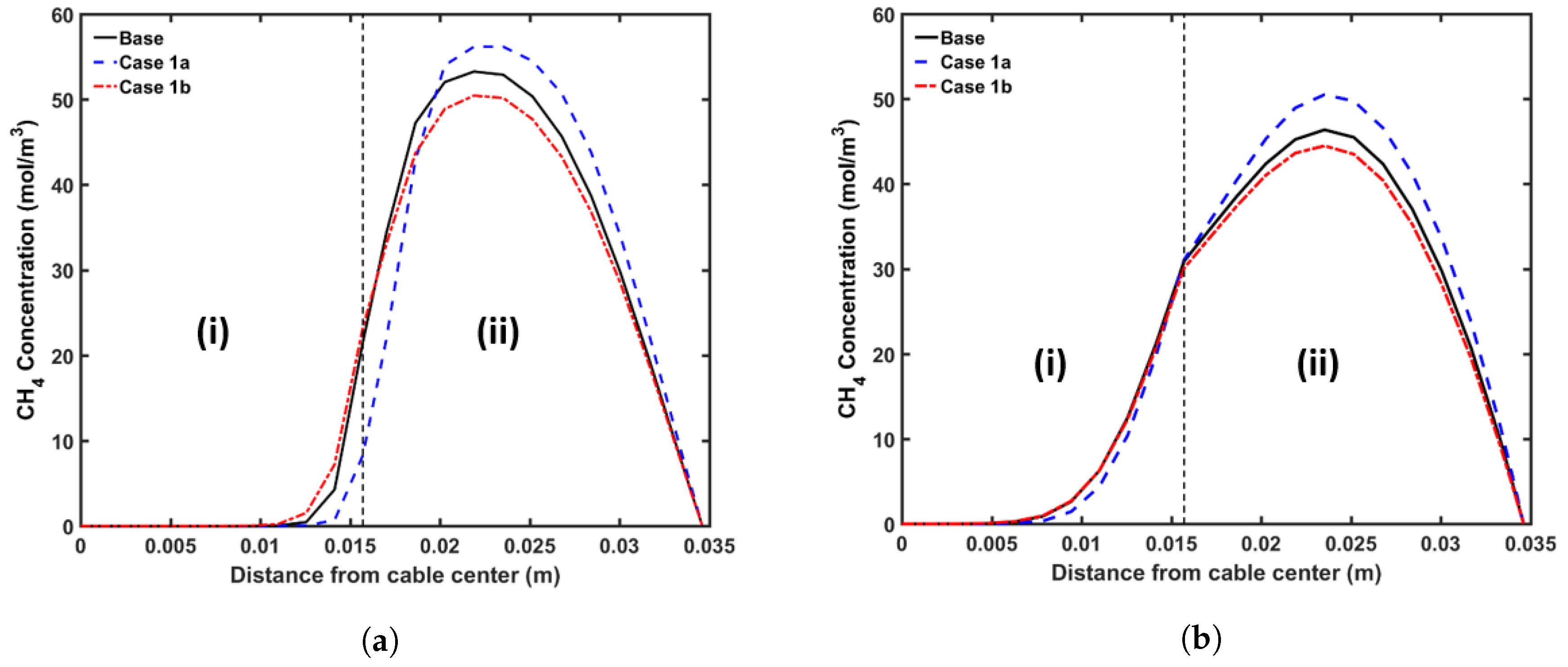
Figure 12.
Radial CH4 concentration profile for the curing temperature study at (a) the curing tube exit, (b) the cable take-up point. Segment (i) corresponds to the conductor layer and segment (ii) corresponds to the cross-linked polyethylene (XLPE) and semiconductor (SC) layers.
Figure 12.
Radial CH4 concentration profile for the curing temperature study at (a) the curing tube exit, (b) the cable take-up point. Segment (i) corresponds to the conductor layer and segment (ii) corresponds to the cross-linked polyethylene (XLPE) and semiconductor (SC) layers.
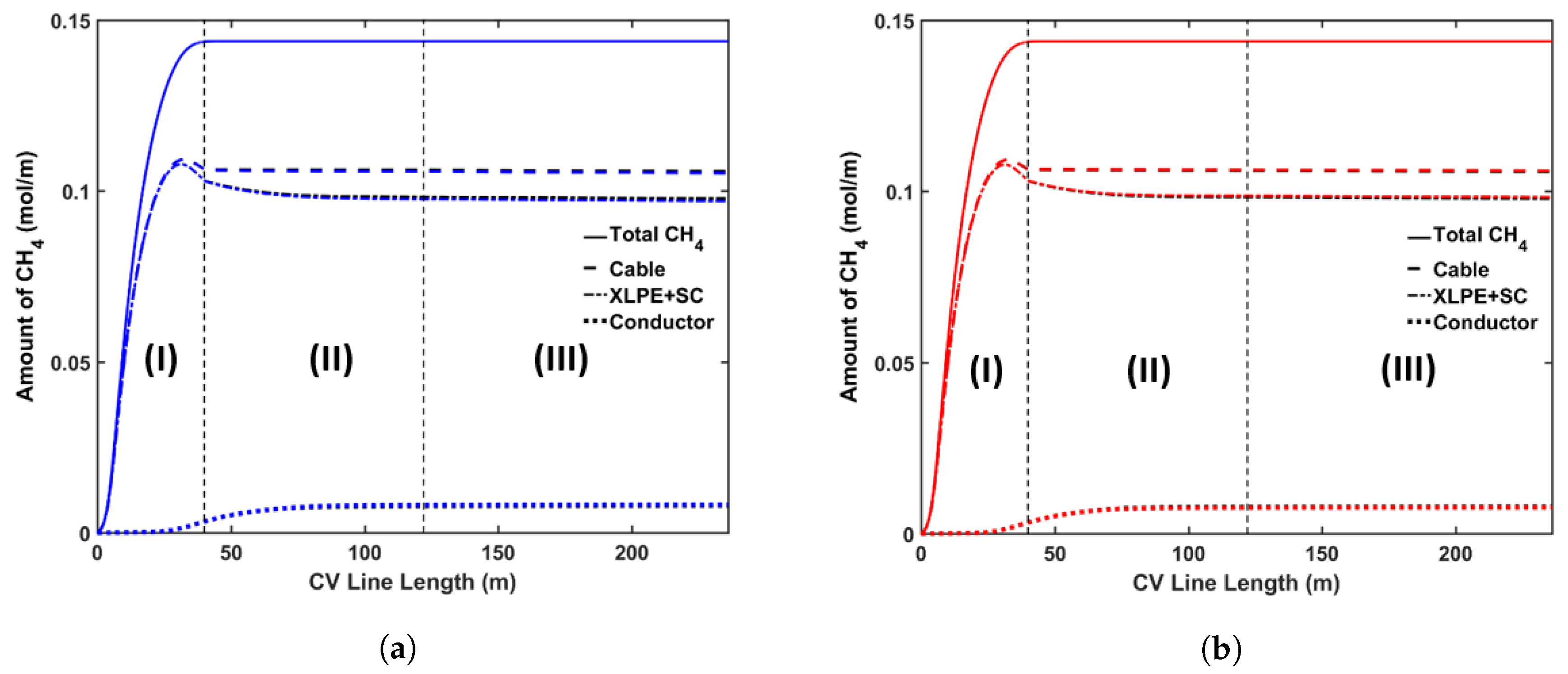
Figure 13.
Axial CH4 concentration profile across the CV line for the line speed study. The black line represents the base case, the blue line in (a) represents Case 2a, and the red line in (b) represents Case 2b. Segments (I), (II) and (III) correspond to the curing tube and transition zone, water-cooling, and air-cooling segments, respectively.
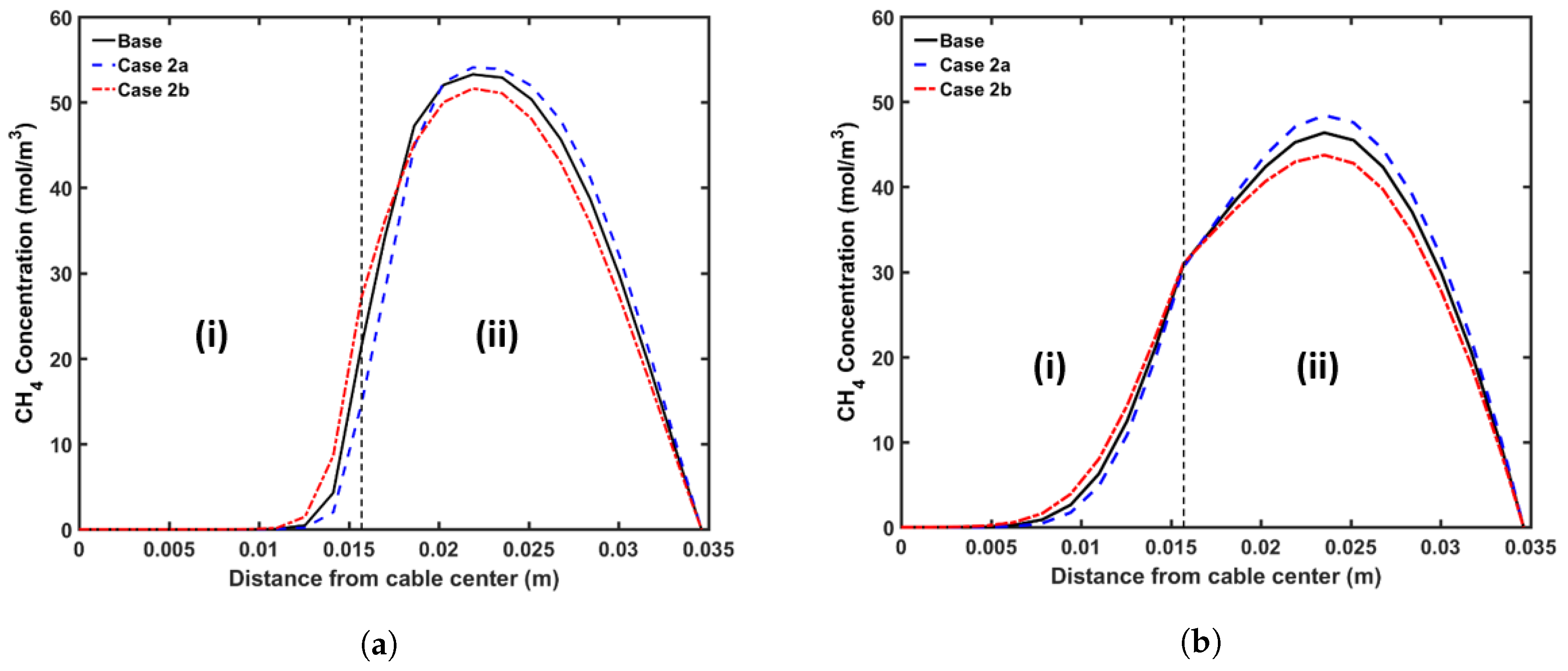
Figure 14.
Radial CH4 concentration profiles for the line speed study at (a) the curing tube exit, (b) the cable take-up point. Segment (i) corresponds to the conductor layer and segment (ii) corresponds to the XLPE and SC layers.
Figure 14.
Radial CH4 concentration profiles for the line speed study at (a) the curing tube exit, (b) the cable take-up point. Segment (i) corresponds to the conductor layer and segment (ii) corresponds to the XLPE and SC layers.
Figure 15.
Axial CH4 concentration profiles across CV line for cooling-water flow rate study. The black line represents the base case, the blue line in (a) represents Case 3a, and the red line in (b) represents Case 3b. Segments (I), (II) and (III) correspond to the curing tube and transition zone, water-cooling, and air-cooling segments, respectively.
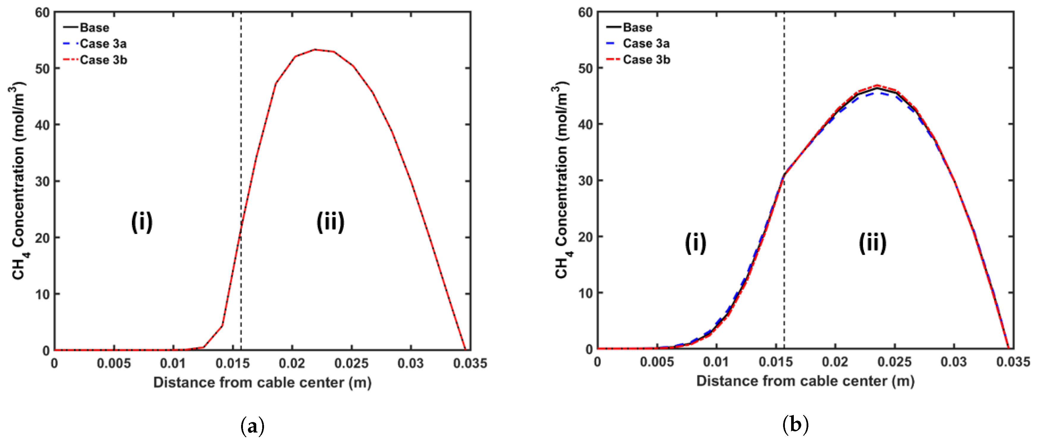
Figure 16.
Radial CH4 concentration profile for cooling-water flow rate study at (a) curing tube exit, (b) cable take-up point. Segment (i) corresponds to conductor layer and segment (ii) corresponds to the XLPE and SC layers.
Figure 16.
Radial CH4 concentration profile for cooling-water flow rate study at (a) curing tube exit, (b) cable take-up point. Segment (i) corresponds to conductor layer and segment (ii) corresponds to the XLPE and SC layers.
Table 1.
Continuous vulcanization (CV) line configuration.
Table 1.
Continuous vulcanization (CV) line configuration.
| Section | Curing Tube | Transition Zone | Water Cooling (1st Section) | Air Cooling |
|---|
| Length (m) | 36 | 4 | 82 | 115 |
Table 2.
CV line operating condition.
Table 2.
CV line operating condition.
| Parameter | Cable Inlet Temp. | Curing Temp. | Line Speed | Water Flow Rate | Water Inlet Temp. |
|---|
| Operating condition | 130 °C | 300 °C | 1.6 m·min | 3 mh | 25 °C |
Table 3.
Computed kinetic parameters for hydrogen abstraction reaction.
Table 3.
Computed kinetic parameters for hydrogen abstraction reaction.
| Data Source | (kJ·mol) | (L·mols) |
|---|
| Rado [28] | 1.8 | |
| Garrett [29] | 15.9 | |
Table 4.
Cable thermal and mechanical properties [
3,
18,
20].
Table 4.
Cable thermal and mechanical properties [
3,
18,
20].
| Property | Copper | XLPE | Semiconductor (SC) |
|---|
| Density, (kg·m) | 8960 | 922 | 1050 |
| Specific heat capacity, (J·kgK) | 401 | 2700 | 1950 |
| Thermal conductivity, k (W·mK) | 385 | 0.335 | 0.53 |
Table 5.
Amount of CH (mol/m) present in each cable component at the cable take-up point.
Table 5.
Amount of CH (mol/m) present in each cable component at the cable take-up point.
| Data Source | Conductor | XLPE + SC | Entire Cable | Total Methane |
|---|
| Rado [28] | 0.0055 (5.3%) | 0.0705 (67.4%) | 0.0760 (72.7%) | 0.1046 (100%) |
| Garret [29] | 0.0079 (5.5%) | 0.0978 (68.0%) | 0.1057 (73.5%) | 0.1438 (100%) |
Table 6.
Amount of CH (mol/m) present in each cable component at the cable take-up point.
Table 6.
Amount of CH (mol/m) present in each cable component at the cable take-up point.
| Case Code | Conductor | XLPE + SC | Entire Cable | Total Methane |
|---|
| Base | 0.0079 (5.5%) | 0.0978 (68.0%) | 0.1057 (73.5%) | 0.1438 (100%) |
| 1a | 0.0071 (4.8%) | 0.1069 (71.9%) | 0.1140 (76.7%) | 0.1486 (100%) |
| 1b | 0.0078 (5.7%) | 0.0937 (67.9%) | 0.1014 (73.5%) | 0.1379 (100%) |
Table 7.
Amount of CH (mol/m) present in each cable component at the cable take-up point.
Table 7.
Amount of CH (mol/m) present in each cable component at the cable take-up point.
| Case Code | Conductor | XLPE + SC | Entire Cable | Total Methane |
|---|
| Base | 0.0079 (5.5%) | 0.0978 (68.0%) | 0.1057 (73.5%) | 0.1438 (100%) |
| 2a | 0.0072 (5.0%) | 0.1022 (71.1%) | 0.1094 (76.1%) | 0.1438 (100%) |
| 2b | 0.0087 (6.1%) | 0.0926 (64.4%) | 0.1013 (70.4%) | 0.1438 (100%) |
Table 8.
Amount of CH (mol/m) present in each cable component at the cable take-up point.
Table 8.
Amount of CH (mol/m) present in each cable component at the cable take-up point.
| Case Code | Conductor | XLPE + SC | Entire Cable | Total Methane |
|---|
| Base | 0.0079 (5.5%) | 0.0978 (68.0%) | 0.1057 (73.5%) | 0.1438 (100%) |
| 3a | 0.0082 (5.7%) | 0.0971 (67.5%) | 0.1053 (73.2%) | 0.1438 (100%) |
| 3b | 0.0077 (5.4%) | 0.0983 (68.4%) | 0.1060 (73.7%) | 0.1438 (100%) |

 ,
, 


