3.1. Basic Solution Process
In
Section 2.3, the CCLOP is formulated as a mixed-integer quadratic programming (MIQP) problem, known for its computational intensity. The Benders’ decomposition algorithm is commonly employed for addressing mixed-integer programming problems, particularly when the remaining slave problem, post-determining the values of integer variables in the master problem, is convex [
48]. To address the slow convergence, various acceleration methods like valid inequalities [
51], approximation techniques [
52,
53,
54] have been explored. Among these methods, leveraging valid inequalities derived from a detailed analysis of the problem [
55] has proven effective in enhancing the convergence of Benders’ decomposition.
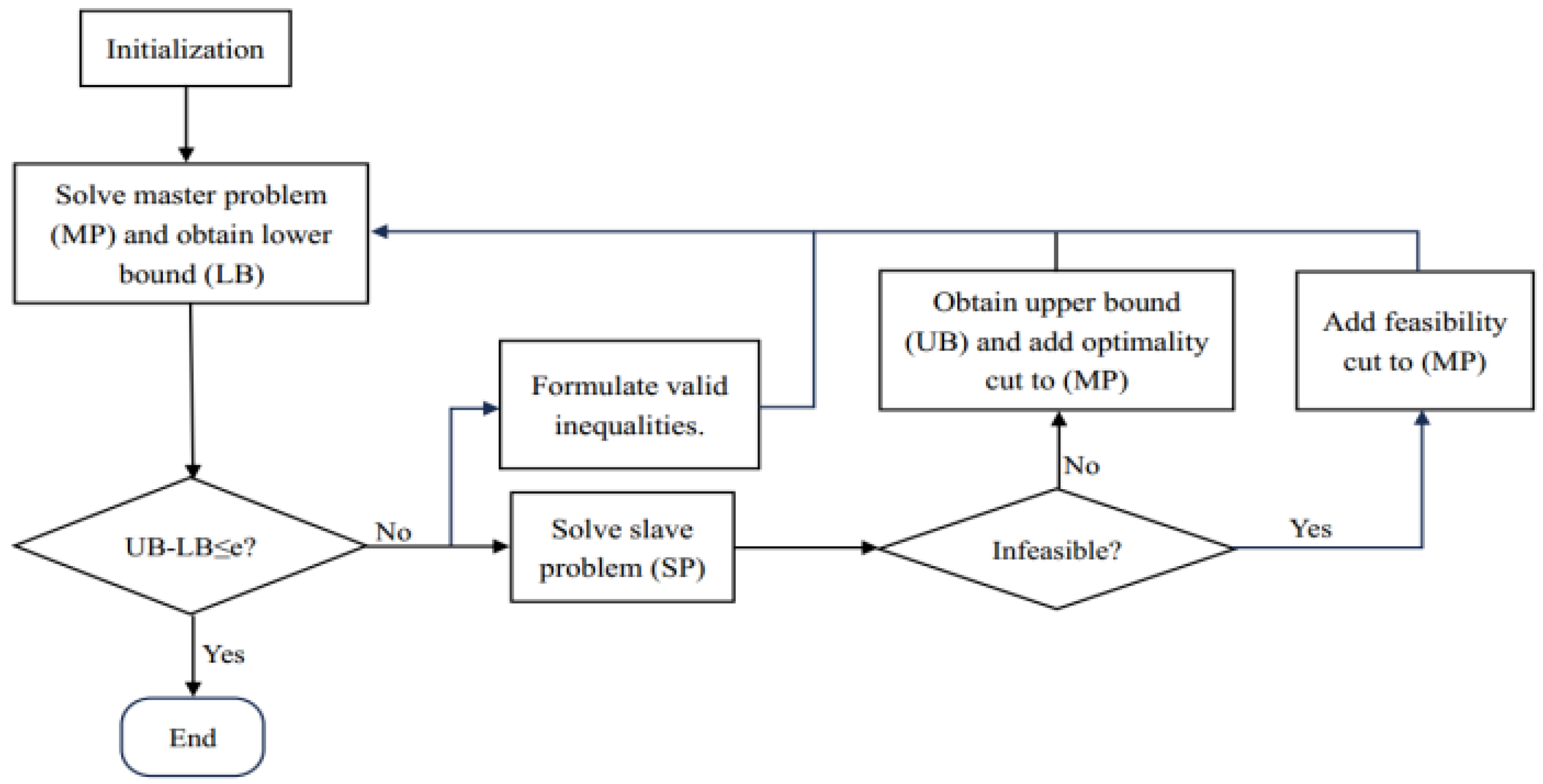
Benders’ decomposition entails partitioning the problem into a master and slave problem. The process, as illustrated in
Figure 3, starts by solving the slave problem separately. Two types of cuts, either Feasibility or Optimality, will be incorporated into the master problem based on the feasibility of the outcomes. The master problem is then addressed to determine the integer variables for the next iteration and obtain a lower bound. The termination criterion is dictated by the difference between the upper and lower bounds. The primal MIQP problem can be represented as:
In the primal problem (P), the continuous variables
are non-negative, thus the vector
comprises non-negative values, and p represents the size of the vector x. Additionally, the vector
comprises binary variables, and
q is the size of the vector
y. Equation (17) represents the equivalent expression of Equations (13)–(15), which combines integer variables in
y and continuous variables in x. Then, Equation (18) defines the feasible set of integer variables in
y, which is equivalent to the expressions given in Equations (4)–(12). When y is fixed, the slave problem (SP) can be formulated as follows:
The fixed value of y, denoted as
, is established either at the start or from the outcome of the master problem in the prior step. The SP is a quadratic programming problem with a convex objective function (19), as the positive semidefinite matrix
H suggests. To solve SP, methods such as interior-point convex algorithms can be employed. These methods facilitate feasibility assessment and yield the Lagrangian multipliers, denoted as
. Here, m represents the present count of derived optimality cuts. On the other hand, an extreme ray
is obtained if SP is infeasible [
56], with n representing the present count of derived feasibility cuts. Next, the master problem (MP) can be formulated as follows:
where
is an intermediate continuous variable. Equation (21) represents the objective function of the MP. Equation (22) is utilized in the initial iteration to enforce the constraint that
remains bounded and non-negative throughout the optimization process. This constraint is crucial for maintaining the feasibility of the problem and ensuring meaningful solutions. Equation (23) denotes the optimality cuts obtained from the SP, while Equation (24) represents the feasibility cuts obtained from the SP. The proposed valid inequalities (VI-1) and (VI-2) are linear constraints elaborated in
Section 3.2. The MP is a mixed-integer programming problem that can be solved via the branch-and-bound algorithm.
3.2. Development of Valid Inequalities
The core intuition of the two valid inequalities is to construct high-quality initial spanning tree structures and heuristic hybrid layouts, so as to generate effective optimality cuts and accelerate the convergence of Benders’ decomposition.
(1) VI-1: Based on the optimization results obtained from the master problem (MP), we define the node set as the set of all nodes that are connected to the virtual root r through the OOGP i, where i belongs to the range [1, Ns]. In other words, encompasses predecessors of node i in the anti-arborescence structure, reflecting the configuration represented by . At each iteration, the node set associated with OOGP i may vary. In such cases, we can perform a reoptimization of the cable connection layout using a greedy-based process:
Step 1: After obtaining the optimization results from the MP, we can store the node set associated with each OOGP i. Remove node i from and define it as Set 1, define Set 2 as an empty set (), and then add node i to it. Then, Step 2 to Step 4 will be iteratively performed for i values ranging from 1 to Ns.
Step 2: Define as a set of distances between pairs of nodes. Specifically, it includes distances for which one node belongs to Set 1 and the other to Set 2. Then arrange these distances in increasing order. Choosing the first element , which is the smallest distance, connects a node from Set 1 (denoted as node ) to a node from Set 2 (denoted as node ).
Step 3: If neither node nor node receives power from more than / nodes, remove the node from Set 1 to Set 2. Otherwise, delete the first element and go back to Step 2.
Step 4: Continue with Step 2 and Step 3 until Set 1 becomes an empty set ().
Step 5: Obtain the integer variables
based on the constructed spanning tree structure, then compare the total cost associated with
to the total cost associated with
. If the cost of
is lower, we substitute
into the SP and solve it to obtain the corresponding Lagrangian multiplier
. As
is constructed based on the spanning tree structure, SP is always a feasible problem. Consequently, (VI-1) can be reformulated as an optimality cut:
(2) VI-2: The second valid inequality arises from the hybridization of different cable connection layouts obtained from various iterations, while maintaining the same node set associated with OOGP i. In other words, it takes into account the combination of cable connections from different iterations that share the common set of nodes . This allows for the exploration of alternative cable connection configurations that leverage the best aspects of different layouts while still adhering to the constraints imposed by the fixed node set . The applicability of the second valid inequality depends on the availability of different cable connection layouts for the current node set . This means that if there are no alternative cable connection layouts for the same node set from previous iterations, the second valid inequality may not be applicable. The cable connection layout is reoptimized by a heuristic method:
Step 1: Obtain the cable connection layout associated with from the current MP optimization results . Then, there are three scenarios to be discussed. In the first scenario, if the cable connection layout for is different from previous iterations but shares the same set of nodes, we add it to the layout set and define them as Set . Here, i represents the node set associated with OOGP i, and t denotes the version of predecessors that connect with node i. In the second scenario, if both the cable connection layout and the set of nodes are different from previous iterations, we add the new layout to the Set . In the final scenario, if both the cable connection layout and the set of nodes have already been covered in previous iterations, there is no need to consider the heuristic process for this particular scenario.
Step 2: If there are multiple OOGPs whose node sets, , meet the first scenario (where the layout is different, but the set of nodes is the same compared to previous iterations), a random selection is made among them to perform the hybridization process.
Step 3: Randomly select one of the layouts from Set and replace the current layout in . The selection process favors layouts with lower total costs, assigning them a higher probability of being chosen. Here, we denote the layout cost of Set as Set , create an intermediate set , and then apply the softmax function to obtain the probability set , ensuring that layouts with lower costs have higher probabilities.
Step 4: If an improved solution is found after replacing the cable connection layout in Step 3, proceed to select a new OOGP in Step 2 and repeat Step 3. However, if an improved solution is not found, continue randomly selecting new layouts from Set until either an improved outcome is achieved or the specified iteration limit is reached, then proceed to select a new OOGP in Step 2 and repeat Step 3.
Step 5: Once the heuristic process has traversed all OOGPs that meet the first scenario, the reoptimized integer variables
are obtained based on the constructed spanning tree structure. The total cost associated with
is then compared to the total cost associated with
. If the cost of
is lower,
is used in the SP, and the problem is calculated to find the corresponding Lagrangian multiplier
. Since
is constructed based on the spanning tree structure, the SP is always a feasible problem. Therefore, (VI-2) can also be reformulated as an optimality cut:
Both valid inequalities are generated from feasible spanning tree structures that satisfy all constraints of the original problem. Since they only add optimality cuts (not feasibility cuts), they cannot exclude the true optimal solution but only tighten the feasible region of the master problem.