A Photovoltaic Power Prediction Method Based on Wavelet Convolutional Neural Networks and Improved Transformer

Abstract

The output power of photovoltaic (PV) systems is influenced by various environmental factors, exhibiting strong nonlinearity and non-stationarity, which poses significant challenges for accurate forecasting. To address these issues, this paper proposes a short-term PV power forecasting method based on wavelet convolutional neural networks and an improved Transformer. First, the Complete Ensemble Empirical Mode Decomposition with Adaptive Noise (CEEMDAN) is employed to decompose the original PV power sequence into several intrinsic mode functions (IMFs). Fuzzy entropy is then utilized to evaluate the complexity of each component, and subsequences with similar entropy values are reconstructed to reduce the non-stationarity of the original series. Subsequently, Pearson correlation coefficients and the maximal information coefficient (MIC) are applied to capture both linear and nonlinear relationships between each reconstructed component and meteorological features, enabling the selection of strongly correlated variables. On this basis, a wavelet convolutional network (WTConv) is introduced to perform multi-scale decomposition and frequency-band feature extraction on the reconstructed components by integrating wavelet transform with convolution operations, effectively expanding the receptive field and extracting deep-seated features of the sequences. Finally, an improved iTransformer model is adopted for time-series modeling, leveraging its inverted encoding structure and self-attention mechanism to fully capture long-term dependencies among multivariate variables. The proposed model is validated using actual power data from a PV plant in Ningxia, China, across four seasons. Comprehensive experiments, including ablation studies, comparative analyses, loss function convergence evaluation, and Diebold–Mariano significance tests, are conducted to thoroughly assess the model’s effectiveness and superiority. Experimental results demonstrate that the proposed model achieves excellent prediction accuracy and stability in spring, summer, autumn, and winter, showing strong potential for engineering applications.

1. Introduction

With the global energy transition and the widespread adoption of renewable energy, the International Energy Agency (IEA) has set a target in its World Energy Outlook for global installed photovoltaic (PV) capacity to reach approximately 16,000 gigawatts (GW) by 2050. By the end of 2023, China’s PV power generation capacity had reached 610 million kilowatts, establishing PV power generation as a cornerstone of renewable energy [1]. However, PV power generation systems are highly susceptible to environmental factors such as solar irradiance, exhibiting significant randomness, intermittency, uncertainty, and volatility [2,3]. If integrated into the grid on a large scale directly, these characteristics can disrupt scheduling plans and compromise the safe operation of the power grid [4]. Therefore, accurate forecasting of PV power output is crucial for grid dispatchers to reasonably adjust generation schedules and maintain the stable operation of the power system [5].

At present, photovoltaic (PV) power forecasting can be primarily categorized into physical methods, direct forecasting methods, and artificial intelligence (AI) methods [6,7]. Physical methods establish models based on photoelectric theory to predict power output, an approach that does not rely on historical PV output data. However, due to the high complexity of factors influencing solar irradiance, current theoretical models are difficult to apply directly to practical scenarios [8]. Direct forecasting methods establish a mapping relationship between historical and future PV output data by analyzing characteristics such as the periodicity and trends of PV power output curves [9]. With the rise in AI methods, data-driven PV power forecasting approaches have been widely applied [10]. Zhang et al. [11] propose a multi-quantile photovoltaic power forecasting model based on a Bidirectional Temporal Convolutional Network. By using the K-means algorithm for same-day weather clustering and integrating quantile regression, the model unifies point and interval forecasting within a single framework, thereby enabling reliable uncertainty quantification and improving prediction accuracy. Deng et al. [12] employ a Long Short-Term Memory (LSTM) model to conduct long-term power generation forecasting for high-rise Building-Integrated Photovoltaic (BIPV) systems, emphasizing the importance of the LSTM model in improving the reliability and efficiency of long-term solar forecasting. Literature [13] adopts a Convolutional Graph Neural Network to mine the spatial correlation features among distributed photovoltaic nodes, highlighting the advantages of this deep learning architecture in enhancing the universality of model training and prediction accuracy.

Since single forecasting models struggle to cope with the variability of weather conditions, leading to a decline in their generalization ability and prediction accuracy, researchers have proposed solutions such as ensemble forecasting models. Nadour et al. [14] combined a convolutional neural network with a bidirectional long short-term memory network, leveraging the spatial feature extraction capability of CNN and the bidirectional temporal modeling advantage of BiLSTM to achieve high-accuracy photovoltaic power forecasting under the extreme Saharan climate. Zhan et al. [15] constructed a multi-module collaborative hybrid forecasting framework that organically integrates clustering analysis, similar-day matching, variational mode decomposition, a temporal convolutional network-long short-term memory-attention mechanism, and physical information constraints, while adaptively tuning key parameters using the rime optimization algorithm, demonstrating excellent generalization ability across different climatic regions. Wang et al. [16] also adopted a hybrid modeling approach, cascading improved complete ensemble empirical mode decomposition with adaptive noise and variational mode decomposition as a preprocessing module, then building the core prediction module with a temporal convolutional network, a bidirectional gated recurrent unit, and an attention mechanism, and finally introducing an improved crested porcupine optimizer for global hyperparameter optimization, forming a complete hybrid chain from data decomposition to prediction to parameter optimization.

When performing PV power prediction, the input features directly affect the prediction results. Furthermore, PV forecasting often involves variables such as meteorological data, so the input features are multidimensional, which not only affects the power output but also increases the model’s complexity. On the one hand, feature decomposition techniques can be used. Sun et al. [17] utilized the discrete wavelet transform to decompose complex raw time series into multi-band components of varying frequencies. Building upon this, they cascaded continuous sampling and interval down-sampling mechanisms, which allowed them to accurately extract both short-term local fluctuations and long-term evolutionary trends within each frequency band. Meanwhile, Wang et al. [18] applied variational mode decomposition as their primary data-smoothing technique to process clustered photovoltaic sequences. By adaptively breaking down the non-stationary data into multiple discrete sub-modes, they effectively circumvented the endpoint effects that frequently occur in traditional decomposition methods. Building on this, Liang et al. [19] proposed a secondary deep feature decomposition architecture. After employing VMD in the initial layer to extract several intrinsic mode sequences alongside a single residual term, they specifically targeted this residual with complete ensemble empirical mode decomposition with adaptive noise to perform a secondary decomposition. This stepped approach maximized mitigation of the mode-mixing drawbacks inherent in single-decomposition methods. These methods improve prediction accuracy through feature decomposition or reconstruction; however, when handling large-scale, high-dimensional data, the decomposed features may still retain noise or unstable components, ultimately affecting the model’s accuracy and generalization. While the decomposition methods in the aforementioned literature effectively mitigate data non-stationarity, they typically input all decomposed sub-sequences directly into the forecasting model. This direct input approach inevitably leads to a surge in computational complexity and the accumulation of prediction errors from each component.

On the other hand, deep learning can be used to fully explore the features of meteorological factors and photovoltaic power generation, and effectively extract the deep information of the features. Han et al. [20] utilized one-dimensional convolution operations with diverse activation functions to specifically extract various complex dynamic features in electricity load sequences, such as linear monotonic, nonlinear gradual, nonlinear abrupt, and periodic fluctuations. Sheng et al. [21] proposed a feature filtering and adaptive reconstruction module that performs multi-scale, parallel feature extraction by combining spatial and channel reconstruction convolutions with receptive-field attention convolutions, effectively reducing feature redundancy in both spatial and channel dimensions. Liu et al. [22] utilized convolution kernels to conduct local spatial scanning on long-term time-series three-dimensional matrices containing multi-dimensional meteorological factors, extracting high-dimensional spatial features at both shallow and deep levels, and employed pooling layers for dimensionality reduction to decrease computational parameters. However, these methods fail to account for information at different data frequencies, and multiple feature-extraction and dimensionality-reduction operations may lead to high computational complexity. Although the aforementioned frameworks are adept at extracting spatial–temporal features, they rely on static, single-scale convolution kernels and fail to dynamically separate macroscopic meteorological trends from transient power fluctuations across different frequency domains, resulting in severely restricted receptive fields.

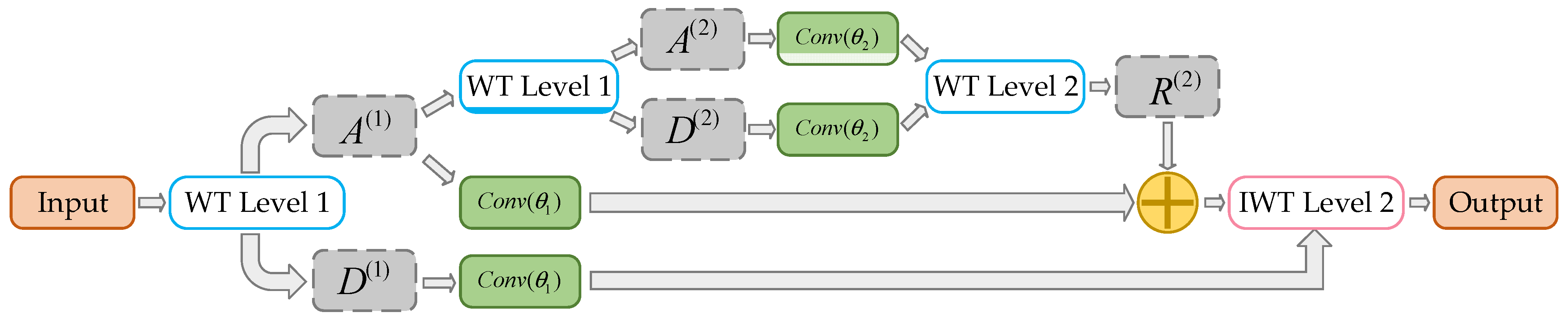
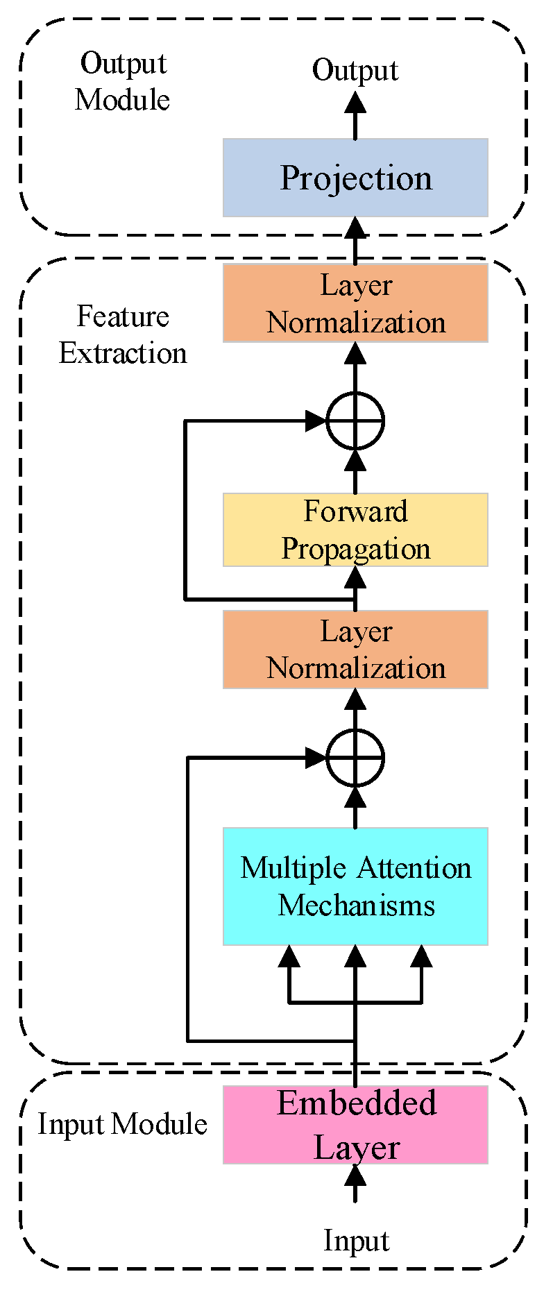
To address the limited forecasting accuracy stemming from limitations of existing photovoltaic models, such as error accumulation from over-decomposition, restricted receptive fields in convolutional networks, and dimensional confounding among covariates, this paper proposes a robust short-term forecasting framework. First, unlike conventional direct decomposition prediction frameworks, we introduce fuzzy entropy to quantify and reconstruct CEEMDAN-derived IMFs. This fundamentally prevents the computational surge and error accumulation caused by over-decomposition, providing highly analyzable and stationary sub-sequences for subsequent deep learning layers. Second, overcoming the limited receptive fields of standard CNNs, we introduce the WTConv module. By seamlessly embedding discrete wavelet transforms into convolution operations, it dynamically extracts frequency-band features, thereby mathematically isolating low-frequency climate trends from high-frequency chaotic noise at minimal parameter cost. Finally, to resolve the dimensional confounding inherent in standard forecasting networks, we adopt the iTransformer. Its inverted encoding structure treats the entire temporal evolution of each meteorological factor as an independent token, accurately capturing pure, long-term cross-variable physical dependencies without interference. Extensive experiments, including cross-regional generalization validation and statistical significance tests, confirm that the proposed framework achieves highly superior forecasting results in terms of robustness, accuracy, and stability.

2. Methodology

2.1. Sequence Decomposition and Feature Reconstruction

2.1.1. Fully Adaptive Noise Ensemble Empirical Modal Decomposition

Completely adaptive ensemble empirical modal decomposition of noise (CEEMDAN) is an optimization and improvement of the empirical modal decomposition (EMD) and ensemble empirical modal decomposition (EEMD) methods [23,24,25], which is able to effectively overcome the problems of modal aliasing and endpoint effects. As the PV power data show obvious volatility, there are some limitations in direct prediction. With CEEMDAN, the complex PV power time series can be decomposed into several intrinsic mode functions (IMFs), and each IMF represents features at different frequencies, which helps reduce prediction complexity. To illustrate this decomposition process, Figure 1 presents the CEEMDAN decomposition results of the photovoltaic power data in January.

Since CEEMDAN is a data-driven adaptive algorithm, the number of IMFs is not manually configured; instead, it is autonomously determined by the inherent complexity of the original photovoltaic power sequence. Consequently, for the January dataset utilized in this study, the algorithm adaptively extracted exactly eight IMFs. The specific calculation procedure for CEEMDAN is detailed as follows:

Step 1: Add Gaussian white noise with standard normal distribution to the original PV data $x(t)$ to get a new sequence $x_i(t)$:

$$x_i(t)=x(t)+\epsilon {\delta }_i(t), i=1,2,\dots ,K$$

(1)

where $\epsilon$ is the weighting factor of Gaussian white noise; ${\delta }_i(t)$ is the randomly generated Gaussian white noise sequence with standard normal distribution for the $ith$ experiment.

Step 2: Perform an empirical modal decomposition of $x_i(t)$ to obtain the $K$ modal components $I_{MF,1}^i(t)$ and the corresponding residual components $c_i(t)$, taking the $I_{MF,1}^i(t)$ mean value as the first modal component $I_{MF,1}(t)$.

$$I_{MF,1}(t)={\displaystyle \frac{1}{K}}{\displaystyle \sum _{i=1}^K{I}_{MF,1}^i(t)}$$

(2)

$$c_1(t)=x(t)-I_{MF,1}(t)$$

(3)

where $I_{MF,1}^i(t)$ is $c_1(t)$ the first modal component of the $ith$ decomposition; is the residual component of the first decomposition.

Step 3: After adding noise to the signal at stage $j$, continue and perform the next round of empirical modal decomposition.

$$I_{MF,j}(t)={\displaystyle \frac{1}{K}}{\displaystyle \sum _{i=1}^K{E}_1\left\{c_{j-1}(t)+{\epsilon }_{j-1}{E}_{j-1}\left[{\delta }_i(t)\right]\right\}}$$

(4)

$$c_j(t)=c_{j-1}(t)-I_{MF,j}(t)$$

(5)

where $I_{MF,j}(t)$ is the $jth$ modal component obtained by CEEMDAN decomposition; $E_{j-1}\left[{\delta }_i(t)\right]$-the $(j-1)th$ IMF component after decomposing the sequence; ${\epsilon }_{j-1}$ is the weighting coefficient of Gaussian white noise added by CEEMDAN to the $(j-1)th$ phase signal; $c_j(t)$ is the signal of the $jth$ stage.

Step 4: Repeat step 3 for $n$ times until the residual signal $c_n(t)$ becomes a monotonic function and the next decomposition cannot be performed.

Step 5: The final PV power sequence is obtained.

$$y(t)={\displaystyle \sum _{k=1}^K{I}_{MF,k}(t)}+c_k(t)$$

(6)

where $K$ is the total number of modal components.

2.1.2. Fuzzy Entropy

Fuzzy Entropy (FE) is an improvement of Approximate Entropy and Sample Entropy [26], based on fuzzy set theory, which defines similarity measures by introducing fuzzy affiliation functions. It assesses the complexity of a sequence by analyzing the number of similar patterns in the time series. Specifically, fuzzy entropy reflects the regularity and randomness of the signal by measuring the similarity and uncertainty between neighboring points in the sequence. The larger the value of fuzzy entropy, the more complex the time series. The specific process is as follows:

Step 1: For a given PV power sequence $\left\{u_1,u_2,\dots u_N\right\}$, reconstruct it into a phase space with an embedding dimension of $m$:

$$X(i)=\left[u(i),u(i+1),\dots u(i+m-1)\right]-u_0(i),i=1,2,\dots ,N-m+1$$

(7)

$$u_0(i)={\displaystyle \frac{1}{m}}{\displaystyle \sum _{j=0}^{m-1}u(i+j)}$$

(8)

where $u_0(i)$ is the sequence mean value.

Step 2: Introduction of fuzzy affiliation function:

$$A(x)=\left\{\begin{array}{l}1, \hspace{0.33em}\hspace{0.33em}\hspace{0.33em}\hspace{0.33em}\hspace{0.33em}\hspace{0.33em}\hspace{0.33em}\hspace{0.33em}\hspace{0.33em}\hspace{0.33em}\hspace{0.33em}\hspace{0.33em}\hspace{0.33em}\hspace{0.33em}\hspace{0.33em}\hspace{0.33em}\hspace{0.33em}\hspace{0.33em}\hspace{0.33em}\hspace{0.33em}\hspace{0.33em}\hspace{0.33em}\hspace{0.33em}\hspace{0.33em}\hspace{0.33em}x=0\\ \exp \left[-\ln (2){\left({\displaystyle \frac{x}{r}}\right)}^2\right],\hspace{0.33em}x>0\end{array}\right.$$

(9)

where $r$ is the similarity threshold.

Step 3: Calculate the maximum distance $d_{ij}^m$ and similarity $A_{ij}$ between any two reconstructed vectors:

$$d_{ij}^m=d\left[X(i),X(j)\right]=\underset{p=1,2,\dots m}{\max }(\left|u(i+p-1)-u_o(i)\right|-\left|u(j+p-1)-u_0(j)\right|)$$

(10)

$$A_{ij}^m=\exp \left[-\ln (2){(d_{ij}^m/r)}^2\right]$$

(11)

where $i,j=1,2,\dots ,N-m$ and $i\ne j$.

Step 4: Calculate the average value of each $i$:

$$M_i^m(r)={\displaystyle \frac{1}{N-m}}{\displaystyle \sum _{j=1,j\ne i}^{N-M+1}{A}_{ij}^m}$$

(12)

Step 5: Define the function:

$$Q^m(r)={\displaystyle \frac{1}{N-m+1}}{\displaystyle \sum _{i=1}^{N-m+1}{M}_i^m}(r)$$

(13)

Step 6: Define the original time series fuzzy entropy:

$$FuzzyEn(m,r)=\underset{N\to \infty }{\lim }\left[\ln Q^m(r)-\ln Q^{m+1}(r)\right]$$

(14)

When the value of the time series is limited, the fuzzy entropy can be estimated by the following method:

$$FuzzyEn(m,r,N)=\ln Q^m(r)-\ln Q^{m+1}(r)$$

(15)

2.2. WTConv-iTransformer Architecture

2.2.1. Wavelet Transform

Wavelet Transform (WT) is an analysis method based on the concept of localization of the Fourier Transform [27,28], which overcomes the limitation that the window size does not vary with frequency in the Fourier Transform, and has the advantages that the Fourier Transform cannot match when dealing with non-smooth signals. Its main features are highlighting the key features of the problem via the transform, performing local time–frequency analysis, decomposing the signal into wavelet functions at different scales and positions, and achieving layer-by-layer refinement of the signal through stretching and translation operations [29]. As a function with local characteristics, the wavelet transform can effectively capture the instantaneous characteristics of the signal and perform local transformations in time and frequency to extract feature information from the digital signal. The formula of the wavelet transform is as follows:

$$W(a,b)={\displaystyle \frac{1}{\sqrt{\left|a\right|}}}{\displaystyle {\int }_{-\infty }^{\infty }f(t)}\psi ({\displaystyle \frac{t-b}{a}})dt$$

(16)

where $W(a,b)$ are Transform coefficients at scale and position $b$, as a result of the transform; $f(t)$ is the Original signal; $\psi (t)$ is the Base wavelet.

2.2.2. Wavelet Convolutional Neural Network

Although the PV power data is decomposed using CEEMDAN for noise reduction and reconstruction, it remains closely related to weather variations, with inherent complexity and uncertainty. Wavelet Transform Convolutional Neural Network (WTConv) [30] utilizes the Wavelet Transform (WT) to process signal features at multiple scales. WTConv allows the signal to be further refined at different scales by secondary decomposition of the reconstructed components in the convolutional layer, and the features are extracted by convolving different frequency components. Different frequency components are convolved to extract features, thus capturing multiple receptive fields and preserving important information in each frequency band.

Each layer of the convolution operation not only captures the overall trend of the signal but also highlights instantaneous changes and local features. The low-frequency component mainly captures the overall trend of the signal, while the high-frequency component emphasizes the rapid changes in the signal. This multi-layer feature extraction approach enables the network to better handle the dynamic nature of PV power data, thereby improving prediction accuracy.

To mathematically formalize this multi-scale feature extraction process and to deeply mine hidden patterns across different time scales without significantly increasing parameter complexity, this paper introduces the following frequency-band decomposition and stepped reconstruction mechanism.

Given the input fused feature sequence or feature map $F_{in}$, we define it as the initial approximation component, i.e., $A^{\left(0\right)}=F_{in}$. In the $kth$ level of frequency band decomposition, the model employs the Discrete Wavelet Transform to decouple the low-frequency approximation component $A^{\left(k-1\right)}$ from the previous layer into a macroscopic low-frequency trend $A^{\left(k\right)}$ and high-frequency details $D^{\left(k\right)}$ that portray local sudden changes:

$$A^{(k)},D^{(k)}=WT(A^{(k-1)})$$

(17)

Once the disparate frequency bands are isolated, the model deploys lightweight convolution operators parameterized by independent network weight sets ${\theta }^{(k)}$ for each corresponding component. This process enables the network to track the long-term periodic evolution of the PV sequence in the low-frequency space, while simultaneously capturing short-term oscillations caused by factors like cloud cover in the high-frequency space:

$${\tilde{A}}^{(k)},{\tilde{D}}^{(k)}=Conv{\theta }^{(k)}(A^{(k)},D^{(k)})$$

(18)

where ${\tilde{A}}^{(k)}$ and ${\tilde{D}}^{(k)}$ represent the mapped low-frequency and high-frequency tensors, respectively. To seamlessly consolidate these cross-band spatial features, the model utilizes the Inverse Wavelet Transform for a bottom–up, step-by-step aggregation. Assuming the maximum decomposition level is $K$ and initializing the boundary condition as $R^{(K+1)}=0$, the reconstructed feature $R^{(K)}$ at the $kth$ level can be calculated by fusing the extracted low-frequency information, high-frequency details of the current layer, and the structural feedback from deeper layers:

$$R^{(k)}=IWT({\tilde{A}}^{(k)}+R^{(k+1)},{\tilde{D}}^{(k)})$$

(19)

The final output response of the system is $F_{out}=R^{(0)}$. Through cascaded decomposition, sub-band mapping, and stepped reconstruction, the network can effectively capture the global evolutionary rules and transient features of PV power at an extremely low parameter count, substantially boosting the model’s generalization capability under complex environmental variations. Figure 2 shows the architecture diagram of the cascaded decomposition and stepped reconstruction in WTConv.

2.2.3. Improved Transformer Model

Existing Transformer models have difficulty in describing correlations between multivariate variables, which limits the model from capturing key features and is less suitable for multivariate time series forecasting [31]. iTransformer is a new model based on Transformer for time series forecasting [32], which embeds the entire temporal evolution of each independent variable as a unified token, rather than fusing multiple variables from the same time step into a single token. It then captures multivariate correlations through self-attention and uses layer normalization and feed-forward network modules to learn better global representations of the series for time series forecasting, addressing the shortcomings of the Transformer forecasting model. The framework consists of an input module, a feature extraction module, and an output module, as shown in Figure 3.

(1)

In the input module, the multivariate time series is embedded individually as a marker with the formula:

$$h_n^0=Embedding(X_{:},n)$$

(20)

where $X_{:},n$ are historical time series; $h_n^0$ represents for embedding markers; $Embedding$ are embedding operations.

(2)

The feature extraction module is composed of multiple stackable Transformer encoder sections, including a multi-head attention mechanism, a forward propagation layer, and a layer normalization operation. The forward propagation layer, i.e., the fully connected layer, is used to avoid model overfitting. Layer normalization is used to reduce the variance between each variable, which is calculated as follows:

$$LayerNorm(H)=\left\{\left.{\displaystyle \frac{h_n-Mean(h_n)}{\sqrt{Var(h_n)}}}\left| n=1,\cdots ,N\right.\right\}\right.$$

(21)

where $H$ is the matrix to be normalized; $h_n$ is the $nth$ sequence in the matrix; $Mean$ is the mean value; $Var$ is the variance.

The following discussion focuses on the multi-head attention mechanism.

Widely used in the field of Natural Language Processing (NLP), the attention mechanism enables a model to capture the interrelationships between positions in a sequence when processing sequence data [33,34]. At its core, it outputs a weighted sum using the corresponding attention weights, calculated from the input sequence’s weight distribution, thereby assigning higher weights to the more relevant elements.

In iTransformer, the attention weights are calculated using $Q$ vectors and $K$ keys, and the $V$ vectors are weighted and summed and output. The attention formula is as follows:

$$Attention(Q,K,V)=Soft\max ({\displaystyle \frac{Q{K}^t}{\sqrt{d_k}}})V$$

(22)

where $Soft\max$ is the Normalization function; $Q$ is the Query vector; $K$ is the Value vector; $V$ is the Primary key vector; $d$ is the Dimension vector; $1/\sqrt{d_k}$ is the Scaling factor, which is used to prevent the gradient from disappearing.

In order to improve the model capability, Transformer is computed in parallel using a multi-head attention mechanism with the following formula:

$$Multih(Q,K,V)=concat(h_1,h_2,\cdots ,h_d)W^O$$

(23)

$$H_s=Attention(Q{W}_S^Q,K{W}_S^K,V{W}_S^V)$$

(24)

where $concat( )$ represents the splicing function; $H_S$ is the $sth$ self-attention function; $W^O$ is the linear mapping matrix of the multi-head attention function; $W_S^Q$, $W_S^K$, $W_S^V$ are the $sth$ first self-attention weight matrix.

(3)

In the output module, it is a linear layer implemented by a multilayer perceptron (MLP), which is used to transform the processed multivariate labels into predicted time series.

2.3. Overall Flow of the Proposed Model

The flowchart of the model proposed in this paper is shown in Figure 4 and is mainly composed of four parts: data decomposition and reconstruction, correlation analysis, a combined prediction model, and analysis of experimental results. Firstly, CEEMDAN is used to decompose the original PV power sequence into multiple intrinsic mode functions (IMFs), and the complexity of each IMF is assessed by calculating its fuzzy entropy. The IMFs are then reconstructed by superimposing subsequences with approximate entropy values (IMFs). Next, the Pearson correlation coefficient and the MIC correlation coefficient between each reconstructed component and the influence features are analyzed simultaneously to capture both linear and nonlinear relationships. Then, a wavelet convolutional neural network is used for feature extraction of the strong correlation influence features and the reconstruction components, in which wavelet variations are combined with convolution to achieve the quadratic decomposition of the reconstruction components, and the application of kernel convolution in different frequency bands increases the sensory field of the neural network and effectively mines the deeper features of the sequences; and the improved Transformer model is used to capture the long term dependencies in the PV power data, and dynamically focus on important time periods to further enhance the prediction effect. Finally, the predicted reconstructed components are superimposed and summed; four evaluation indices are used to verify the model’s effectiveness, and several experiments are conducted to further demonstrate the model’s superiority in this paper.

3. Case Analysis

3.1. Experimental Data and Platform

The experimental data used in this study were collected from a photovoltaic power station in Ningxia, China, covering January, April, July, and October of 2019, which represent the four seasons of spring, summer, autumn, and winter, respectively, in order to validate the effectiveness and generalization capability of the proposed model. The dataset exhibits typical temporal characteristics of photovoltaic power generation, showing a clear diurnal cycle. Specifically, the power output is nearly zero during nighttime, while significant fluctuations occur during daytime. The maximum output power is approximately 128 MW, and the standard deviation is 34.59, indicating strong variability and pronounced non-stationarity in the data. Given the intermittency of photovoltaic power generation, data from 8:00 to 22:00 were selected with a 15 min sampling interval. The influencing factors include 16 variables, such as air temperature, air pressure, humidity, dew point temperature, and solar radiation.

To preserve the chronological integrity of the time series, the data for each selected month are sequentially partitioned into training, validation, and test sets in a 7:1:2 ratio. Furthermore, data preprocessing procedures, including normalization and feature selection, are applied exclusively to the training set to prevent potential data leakage. During model training, the Mean Squared Error (MSE) is used as the loss function to quantify the deviation between the forecast and actual photovoltaic power values, and the Adam optimizer is used to adaptively update the network weights. The input sequence length is set to 56-time steps, enabling the model to capture a complete diurnal fluctuation cycle. Concurrently, the forecasting horizon is set to 1 time step, enabling 15 min ahead short-term predictions.

The experiments were conducted on an experimental platform with an Intel Core i9-11900K processor, NVIDIA GeForce RTX 3080 GPU, and 32 GB DDR4 memory.

After constructing the dataset and analyzing its fundamental characteristics, it is necessary to appropriately configure the key hyperparameters of the proposed model to fully exploit its advantages in feature extraction and multivariate modeling. The selection of hyperparameters directly affects the model’s feature representation capability, convergence speed, and prediction accuracy. Consequently, to identify the optimal configuration for the proposed model, the final parameter settings were determined via a systematic grid search method, accounting for the data characteristics and model complexity. The main hyperparameter configurations used in this study are listed in

Table 1. Parameters of the model.

Hyperparameter	WTConv-iTransformer
Wavelet levels	2
Kernel size	3
Embedded dimension	32
Hidden layer dimension	64
Multi-head attention	8
Dropout rate	0.1
Learning rate	0.0001
Batch size	32
Epoch	80

.

3.2. Data Preprocessing and Evaluation Metrics

Outliers can occur during the collection of PV power data, and such data can affect the predictability of the model and reduce the prediction accuracy. Outliers are detected using the 3Sigma rule, which identifies those data points that exceed the range of mean ±3 standard deviations by calculating the mean and standard deviation of the data. Detected outliers are replaced with null values, and then cubic spline interpolation is used to fill these null values.

In order to measure the prediction performance of the model, Root Mean Squared Error (RMSE), Mean Absolute Error (MAE), Mean Absolute Percentage Error (MAPE), and goodness-of-fit were used to analyze the prediction results. The four evaluation metrics were analyzed as follows. The formulas for the four evaluation indexes are as follows:

$$RMSE=\sqrt{{\displaystyle \frac{1}{N}}{\displaystyle \sum _{i=1}^N{({\widehat{y}}_i-y_i)}^2}}$$

(25)

$$MAE={\displaystyle \frac{1}{N}}{\displaystyle \sum _{i=1}^N\left|{\widehat{y}}_i-y_i\right|}$$

(26)

$$MAPE={\displaystyle \frac{1}{N}}{\displaystyle \sum _{i=1}^N\left|\frac{{\widehat{y}}_i-y_i}{y_i}\right|\times 100}\%$$

(27)

$$R^2=1-{\displaystyle \frac{{\displaystyle \sum _{i=1}^N{(y_i-{\widehat{y}}_i)}^2}}{{\displaystyle \sum _{i=1}^N{(y_i-{\overline{y}}_i)}^2}}}$$

(28)

where $N$ are the number of predicted samples; $y_i$ is the $ith$ actual value of the first sample; ${\widehat{y}}_i$ is the $ith$ predicted value of the first sample; ${\overline{y}}_i$ is the average value of the actual sample.

3.3. Sequence Decomposition and Reconstruction

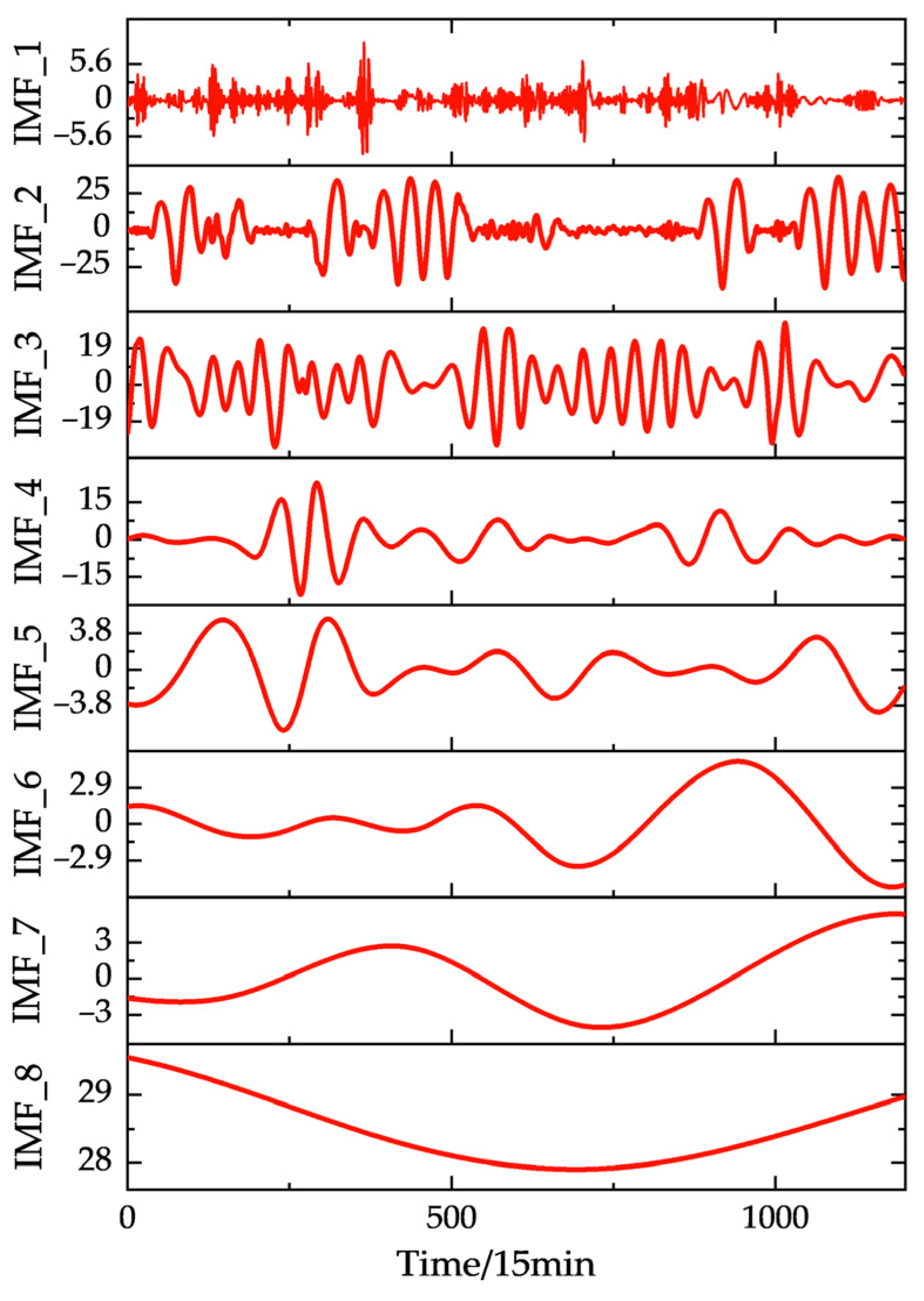
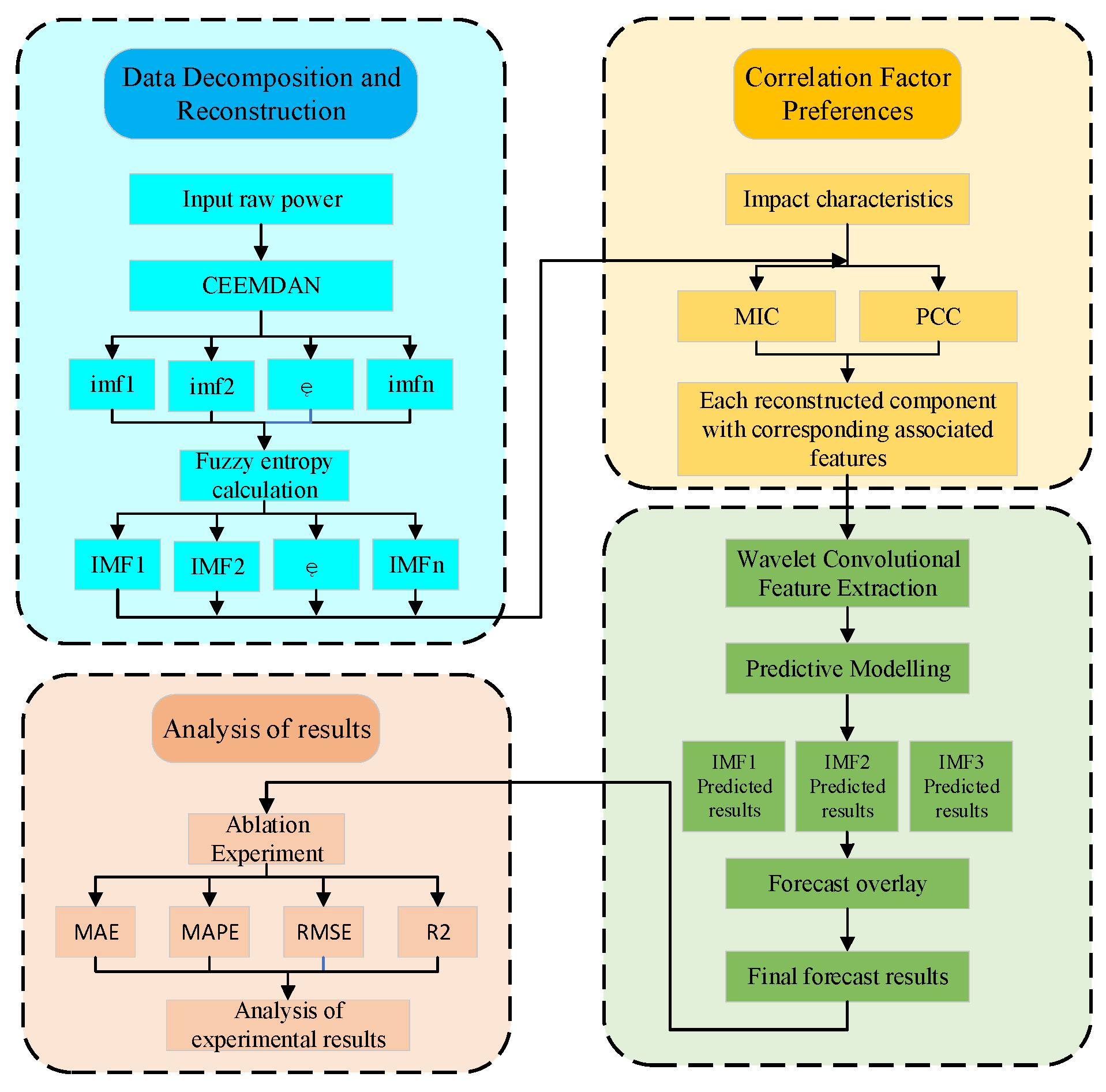
Considering the strong periodicity and uncertainty of the PV power data, CEEMDAN is initially used to decompose the raw data into multiple IMF components. However, establishing independent prediction modules for all generated sub-sequences directly would inevitably lead to a surge in computational complexity and severe error accumulation due to over-decomposition. Therefore, Fuzzy Entropy is introduced to quantify the dynamic complexity and randomness of each individual IMF.

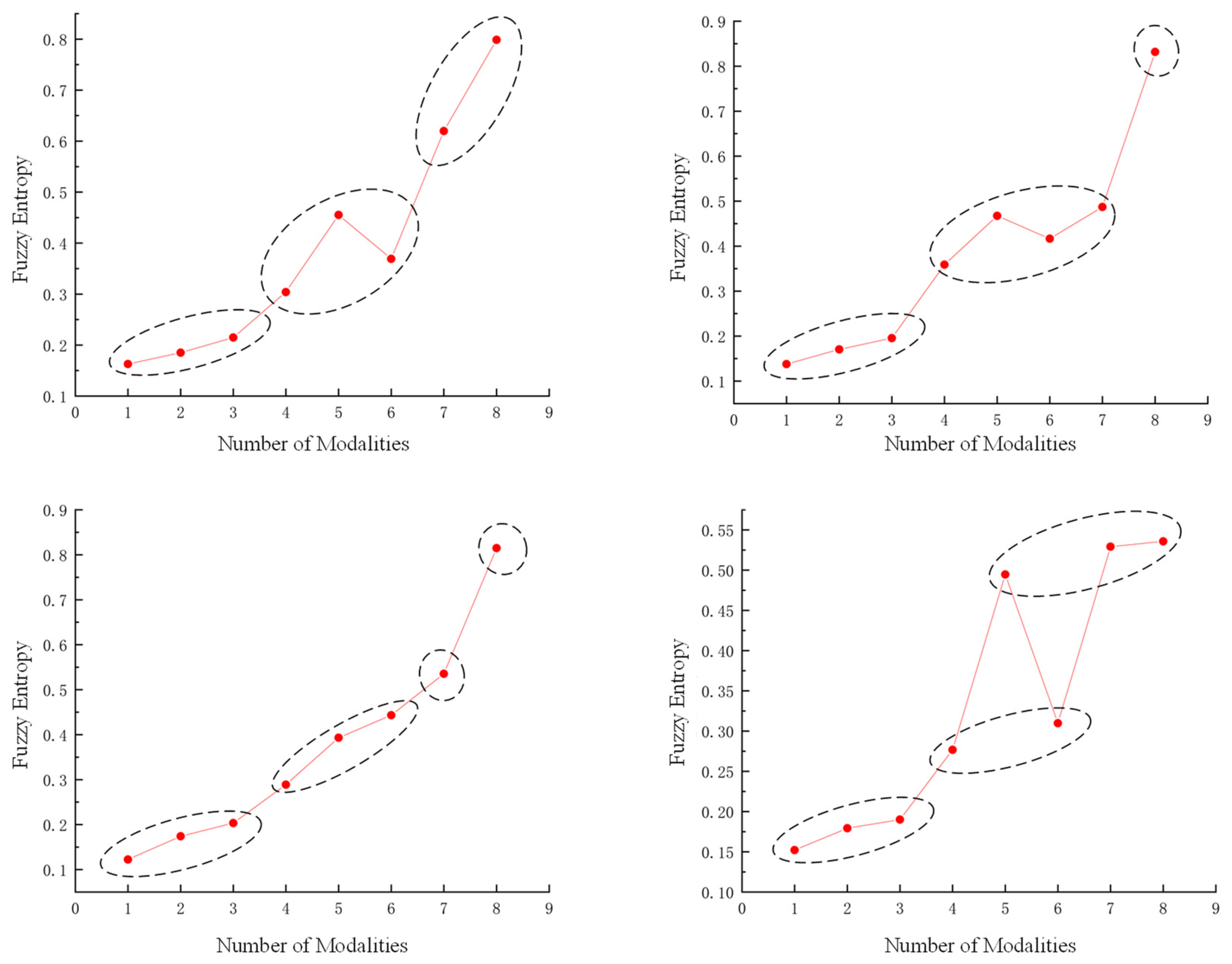
The results of the fuzzy entropy value of PV sequences in January, April, July, and October 2019 are shown in Figure 5. Scientifically, the FE values exhibit a distinctly hierarchical distribution that aligns with the physical characteristics of the PV signals. The initial high-frequency IMFs naturally exhibit the highest FE values, indicating intense stochasticity driven by sudden changes in cloud cover or sensor noise. The intermediate IMFs exhibit moderate FE values, consistent with the macroscopic diurnal cycles. Finally, the low-frequency residual components exhibit FE values approaching zero, reflecting smooth, long-term evolutionary trends.

Rather than merely describing the data, this entropy-based complexity assessment provides a rigorous mathematical criterion for feature compression. By superimposing IMFs with similar entropy magnitudes, subsequences with isomorphic dynamical characteristics are adaptively merged into distinct reconstructed components. This reconstruction strategy effectively mitigates the severe non-stationarity of the original data and significantly alleviates the “curse of dimensionality,” yielding highly analyzable, stationary sub-sequences without discarding any critical frequency-domain information for the subsequent modeling phase.

3.4. Correlation Analysis

Input variables directly impact the model’s predictive ability and are key elements of a PV power prediction model. The input variables should cover sufficient features, and too many meteorological factors may lead to redundant information and reduce model accuracy. Therefore, Pearson correlation analysis was used to determine the linear relationship between PV power and meteorological factors; however, many non-linear, indirect, and deeper relationships exist between the two, so the maximum mutual information coefficient (MIC) was then used for correlation analysis. The threshold value for the correlation coefficient is set to 0.3, and the correlation results for each reconstructed component with meteorological features in January are shown in

Table 2. Correlation between the reconstructed components and meteorological characteristics in January.

Reconstructed Component	Impact Characteristics	Correlation Coefficient
		Pearson	MIC
IMF1	Direct radiation	0.602	0.378
	Total radiation	0.721	0.455
	Fixed inclination radiation	0.703	0.383
	Tracking Inclination Radiation	0.694	0.449
	Zenith angle	−0.657	0.425
IMF2	Scattered radiation	0.465	0.326
	Total radiation	0.674	0.499
	Fixed inclination radiation	0.591	0.413
	Tracking Inclination Radiation	0.615	0.466
	Zenith angle	−0.628	0.438
IMF3	Opacity	−0.469	0.459
	Direct radiation	0.401	0.449
	Fixed inclination radiation	0.319	0.374
	Snow depth	−0.369	0.433

.

The table further reveals significant differences in correlations between reconstructed components and meteorological features. Specifically, for the component IMF1, strong positive correlations are observed with radiation-related variables, while a significant negative correlation is found with the solar zenith angle. This indicates that IMF1 primarily reflects rapid fluctuations in photovoltaic power driven by variations in solar irradiance. For the component IMF2, the overall correlation pattern is similar to that of IMF1, although the correlation coefficients are slightly lower. This suggests that IMF2 retains the dominant influence of radiation factors while also being affected to some extent by other meteorological variables, reflecting relatively smoother variation trends. In addition, the MIC values are generally higher than the corresponding Pearson coefficients, indicating that IMF2 may contain more nonlinear relationships. In contrast, the component IMF3 exhibits a distinctly different correlation pattern. It shows relatively strong correlations with opacity and snow depth, while its linear correlations with radiation variables are significantly weaker. However, the MIC values remain relatively high, suggesting that this component has more implicit nonlinear and indirect influences.

Overall, the differences in correlations among the reconstructed components validate the need to decompose and reconstruct the original sequence. On the one hand, this process transforms complex non-stationary series into sub-sequences with distinct physical meanings; on the other hand, the combined use of Pearson and MIC analysis enables the capture of both linear and nonlinear relationships, thereby providing a more reliable basis for feature selection and multi-scale modeling.

In order to eliminate the differences in physical dimensions, it is necessary to normalize the input variables with the following formula:

$$x^{\prime }={\displaystyle \frac{x-x_{min}}{x_{max}-x_{min}}}$$

(29)

where $x$ are raw data; $x_{min}$ is the minimum value in the data set; $x_{max}$ is the maximum value in the data set; $x^{\prime }$ is normalized value.

3.5. Ablation Experiment

In order to verify the model’s validity, the proposed model is compared with the CEEMDAN-iTransformer model, with the elimination of the feature extraction module to verify the validity of WTConv, and with the WTConv-iTransformer model without CEEMDAN to verify the validity of modal decomposition, and then with the CEEMDAN-WTConv-Transformer model to verify the performance of iTransformer compared to Transformer.

Table 3. Evaluation indicators of each model.

Season	Modelling	${\mathit{R}}^2$	MAE/MW	MAPE/%	RMSE/MW
January	WTConv-iTransformer	0.968	2.183	4.898	3.901
	CEEMDAN-iTransformer	0.976	2.031	4.174	2.863
	CEEMDAN-WTConv-Transformer	0.981	2.014	3.556	3.694
	CEEMDAN-WTConv-iTransformer	0.984	1.832	3.259	2.711
April	WTConv-iTransformer	0.966	4.447	4.018	5.620
	CEEMDAN-iTransformer	0.961	3.625	3.779	5.381
	CEEMDAN-WTConv-Transformer	0.984	3.344	2.736	4.960
	CEEMDAN-WTConv-iTransformer	0.988	3.058	3.181	4.309
July	WTConv-iTransformer	0.979	2.589	4.332	4.181
	CEEMDAN-iTransformer	0.983	2.214	4.308	4.149
	CEEMDAN-WTConv-Transformer	0.989	2.003	4.164	3.569
	CEEMDAN-WTConv-iTransformer	0.995	1.876	3.945	2.937
October	WTConv-iTransformer	0.978	2.356	4.686	2.752
	CEEMDAN-iTransformer	0.989	2.079	3.342	2.580
	CEEMDAN-WTConv-Transformer	0.994	1.965	2.778	2.056
	CEEMDAN-WTConv-iTransformer	0.996	1.310	2.438	1.637

compares evaluation metrics for each model across the ablation experiments conducted in January, April, July, and October. The tables show that the proposed model achieves the best performance across all four seasons for MAE, MAPE, RMSE, and R². Taking January as an example for detailed analysis, the MAE, MAPE, and RMSE of the proposed model are reduced by 9.03%, 8.35%, and 26.56%, respectively, while the R² is improved by 0.31% compared to the CEEMDAN-WTConv-Transformer model. This is because standard Transformers tokenize all variables within a single time step into a unified vector, which blurs the physical independence of different meteorological factors. In contrast, the iTransformer module embeds each variable as an independent token, making it better suited to handling multivariate time-series data. Compared to the WTConv-iTransformer model, the proposed model’s MAE, MAPE, and RMSE are reduced by 16.08%, 33.46%, and 30.5%, respectively, with an R² improvement of 1.65%. This demonstrates that the entropy-based CEEMDAN decomposition, combined with the data reconstruction module, effectively mitigates the highly non-stationary nature of the raw photovoltaic power sequences, thereby substantially enhancing the fitting capability. For the CEEMDAN-iTransformer model, MAE, MAPE, and RMSE are reduced by 9.80%, 21.92%, and 5.31%, respectively, and R² improves by 0.82%. This demonstrates that the WTConv module can expand the receptive field of feature decomposition and acts as a learnable secondary decomposition mechanism. It mathematically isolates meteorological trends in the low-frequency space while sensitively capturing transient power drops in the high-frequency space, thereby continuously providing highly refined multi-scale feature maps for the prediction phase.

A comprehensive analysis of the tables shows that while the improved Transformer contributes to performance gains, its full potential may not be realized within a limited monthly dataset. Conversely, the combination of CEEMDAN and WTConv produces a quadratic decomposition effect that significantly suppresses noise interference in non-stationary sequences, leading to exceptionally high R² values of 0.995 in July and 0.996 in October, thereby substantially boosting the model’s prediction accuracy and fitting stability.

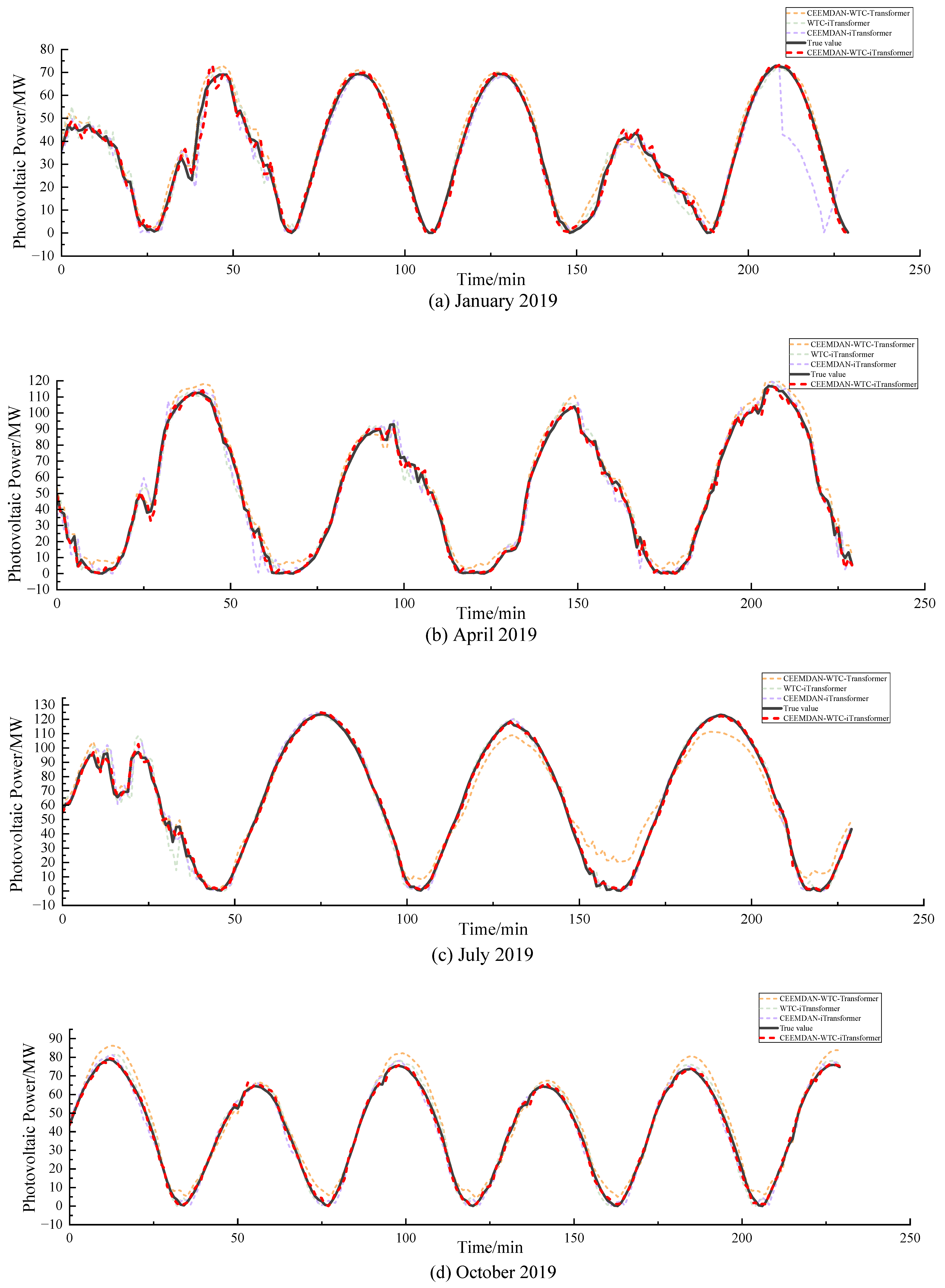
In order to clearly observe the prediction performance of the proposed model and the comparison model, the prediction curves of a certain period in January, April, July, and October are selected, respectively. As shown in Figure 6, the proposed model’s prediction curve is closest to the real value among all models, with the smallest fluctuation range, indicating good prediction accuracy and fitting ability.

3.6. Performance Analysis of the Loss Function

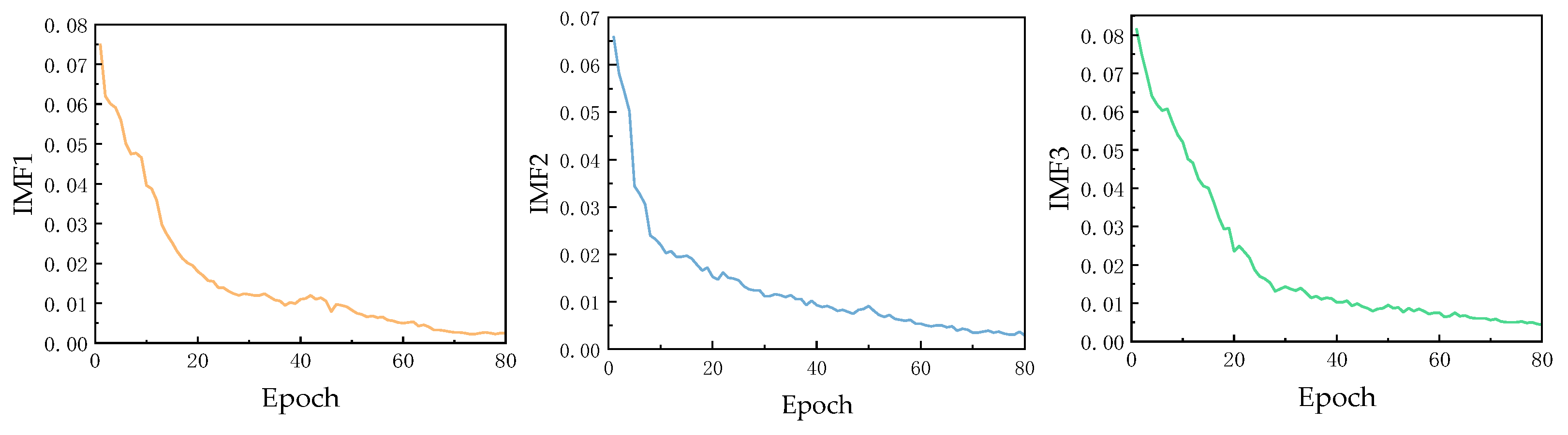
To evaluate the learning performance of the proposed model on the reconstructed components, this paper plots the loss function convergence curves of the reconstructed components during the training process. Taking January as an example, a brief analysis is conducted on the convergence curves of the three reconstructed components: The IMF1 component corresponds to the reconstructed sub-sequence with the lowest complexity; its loss converges at the fastest rate and achieves the lowest final stabilized loss value. This indicates that the model can highly effectively capture and fit the stationary variation patterns inherent in this component. The loss sequences of the IMF2 and IMF3 components also maintain a highly stable downward trend. Due to their greater fitting difficulty, their final stabilized loss values are slightly higher than those of the IMF1 component, which objectively reflects the model’s strong robustness and feature extraction capabilities.

As shown in the overall loss convergence analysis results in Figure 7, the loss values of all components decrease rapidly as the number of training epochs increases, and they generally stabilize after approximately 20 epochs. This phenomenon clearly demonstrates the excellent convergence of the model and fully proves that the proposed model possesses strong, stable learning capability.

3.7. Significance Test

In summary, BiLSTM and CNN-LSTM are constrained by their inherent network structures and fall short in adequately extracting multi-scale time–frequency features from PV power data. Although Transformer and Informer have made progress in long-sequence modeling, they still have limitations in multivariate independent modeling and the effective utilization of frequency information. The proposed model addresses these shortcomings by applying CEEMDAN decomposition to reduce sequence non-stationarity, employing WTConv to extract multi-scale time–frequency features, and leveraging iTransformer for independent multivariate modeling, thereby achieving optimal prediction performance.

To verify the statistical significance of the performance improvement achieved by the proposed model (denoted as model 1) over its ablated variants, the Diebold–Mariano (DM) test is employed to compare the prediction error sequences of different models. The comparison models include CEEMDAN-WTConv-Transformer (denoted as model 2), CEEMDAN-iTransformer (denoted as model 3), and WTConv-iTransformer (denoted as model 4). Pairwise DM tests are conducted on the absolute prediction error sequences for four months: April, July, October, and January.

Table 4. Significance analysis results of different models.

Season	Comparison Models	DM Statistic	p-Value	Significant (α = 0.05)
January	Model 1 vs. Model 2	–4.12	3.78 × 10−5	significantly superior
	Model 1 vs. Model 3	–5.87	4.36 × 10−9	significantly superior
	Model 1 vs. Model 4	–6.33	2.45 × 10−10	significantly superior
April	Model 1 vs. Model 2	–3.98	6.89 × 10−5	significantly superior
	Model 1 vs. Model 3	–4.76	1.93 × 10−6	significantly superior
	Model 1 vs. Model 4	–5.41	6.30 × 10−8	significantly superior
July	Model 1 vs. Model 2	–4.55	5.36 × 10−6	significantly superior
	Model 1 vs. Model 3	–5.12	3.05 × 10−7	significantly superior
	Model 1 vs. Model 4	–6.04	1.54 × 10−9	significantly superior
October	Model 1 vs. Model 2	–4.89	1.00 × 10−6	significantly superior
	Model 1 vs. Model 3	–5.63	1.79 × 10−8	significantly superior
	Model 1 vs. Model 4	–6.78	1.19 × 10−11	significantly superior

shows that for all seasons, the absolute DM statistics between model1 and model 2, model1 and model 3, and model1 and model 4 all exceed the critical values, with corresponding p-values less than 0.001, thereby rejecting the null hypothesis of equal prediction accuracy. This indicates that the contributions of CEEMDAN decomposition and reconstruction, WTConv multi-scale feature extraction, and iTransformer independent variable modeling are all statistically significant and not due to random fluctuations. Therefore, the proposed model outperforms all ablated variants in a statistically significant manner, confirming the effectiveness and robustness of its architectural design.

3.8. Comparative Experiments

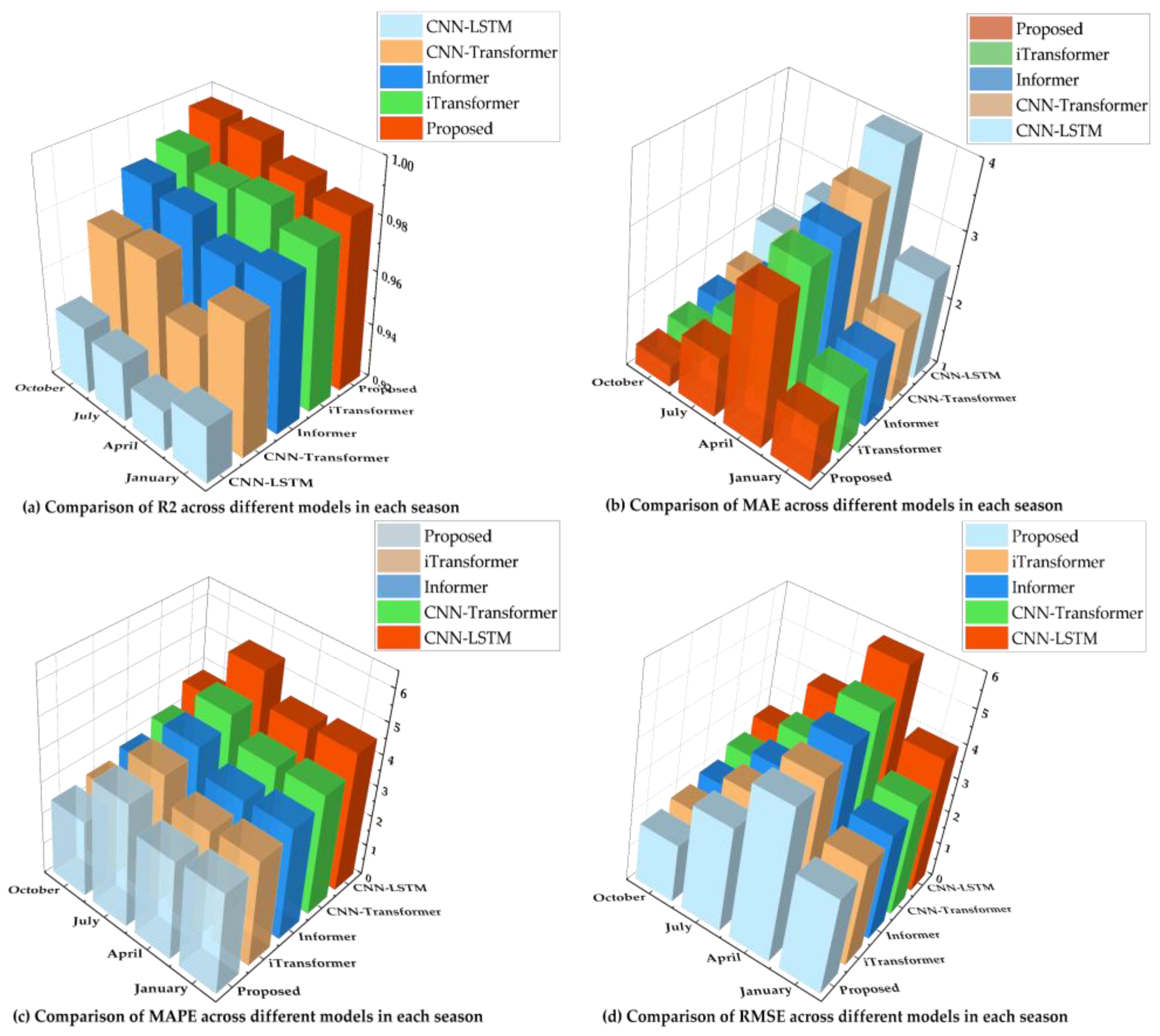
To thoroughly validate the effectiveness of the CEEMDAN-WTConv-iTransformer model proposed in this paper for short-term photovoltaic power forecasting, this section conducts comparative experiments using four classic and widely adopted models in the field of time series forecasting. The experimental results are presented in

Table 5. Forecasting performance metrics in comparative experiments.

Season	Modelling	${\mathit{R}}^2$	MAE/MW	MAPE/%	RMSE/MW
January	CNN-LSTM	0.941	2.512	4.512	3.956
	CNN-Transformer	0.969	2.111	3.908	3.257
	Informer	0.975	2.015	3.612	3.045
	iTransformer	0.980	1.977	3.416	2.902
	Proposed	0.984	1.832	3.259	2.711
April	CNN-LSTM	0.935	4.012	4.415	5.842
	CNN-Transformer	0.954	3.543	3.891	5.072
	Informer	0.972	3.315	3.542	4.715
	iTransformer	0.986	3.219	3.332	4.437
	Proposed	0.988	3.058	3.181	4.309
July	CNN-LSTM	0.942	2.745	5.412	4.156
	CNN-Transformer	0.972	2.331	4.653	3.521
	Informer	0.981	2.105	4.312	3.245
	iTransformer	0.984	1.956	4.117	3.105
	Proposed	0.995	1.876	3.945	2.937
October	CNN-LSTM	0.945	2.015	3.745	2.541
	CNN-Transformer	0.971	1.595	3.158	2.223
	Informer	0.984	1.512	2.815	1.925
	iTransformer	0.989	1.407	2.559	1.762
	Proposed	0.996	1.310	2.438	1.637

, while Figure 8 visually demonstrates the superiority of the proposed method.

A detailed analysis is provided using the January data as an example: The CNN-LSTM model records an R² of 0.941, with MAE, MAPE, and RMSE values of 2.512 MW, 4.512%, and 3.956 MW, respectively. Relative to the proposed model, its MAE and RMSE are 37.12% and 45.92% higher, respectively. Although CNN-LSTM extracts local features through convolutional layers, the use of a single-scale convolution kernel restricts its ability to simultaneously capture fluctuation patterns across different time scales. Moreover, the absence of a dynamic weighting mechanism for input features reduces its adaptability when correlations with meteorological variables change over time. The CNN-Transformer model achieves an R² of 0.969, with MAE, MAPE, and RMSE values of 2.111 MW, 3.908%, and 3.257 MW, respectively. Compared to the proposed model, its MAE and RMSE are 15.23% and 20.14% higher, respectively. While introducing the Transformer architecture improves the modeling of temporal dependencies compared to CNN-LSTM, it still utilizes standard convolution for feature extraction, which limits the receptive field and struggles with complex multi-scale frequency components. Furthermore, it retains the conventional tokenization strategy that blends multivariate variables. The Informer model achieves an R² of 0.975, with MAE, MAPE, and RMSE values of 2.015 MW, 3.612%, and 3.045 MW, respectively. In comparison with the proposed model, its MAE and RMSE are 9.99% and 12.32% higher, respectively. While Informer improves the efficiency of long-sequence forecasting on the basis of Transformer, it still relies on the same tokenization strategy, which imposes constraints when handling complex interactions among multiple variables. It also lacks a dedicated module designed to extract multi-scale frequency features from PV power sequences. The standalone iTransformer model yields an R² of 0.980, with MAE, MAPE, and RMSE values of 1.977 MW, 3.416%, and 2.902 MW, respectively. Compared to the proposed model, its MAE and RMSE are 7.91% and 7.05% higher, respectively. Although the iTransformer successfully addresses the issue of multivariate confounding by treating the entire temporal evolution of each variable as an independent token, its direct application to raw, highly volatile PV sequences without prior noise reduction and multi-scale frequency decomposition limits its ability to reach optimal forecasting accuracy.

In summary, traditional deep learning models like CNN-LSTM are constrained by single-scale feature extraction, while advanced variants like CNN-Transformer and Informer face bottlenecks in multivariate independent modeling and frequency information utilization. Even the advanced iTransformer falls short of its full potential due to the lack of a dedicated data decomposition module. The proposed model successfully addresses these shortcomings by applying CEEMDAN decomposition to reduce sequence non-stationarity, employing WTConv to extract multi-scale time–frequency features, and leveraging iTransformer for independent multivariate modeling, thereby achieving optimal prediction performance.

3.9. Generalization Verification

To evaluate the generalization capability of the proposed model beyond the specific climatic conditions and plant scale of the primary dataset, additional experiments were conducted on the Desert Knowledge Australia Solar Center (DKASC) photovoltaic dataset. This dataset is collected from a PV plant located in a different region, featuring distinct geographical characteristics and meteorological patterns. The variations in installed capacity and localized weather dynamics provide a rigorous test for the spatial robustness of the model.

Following the exact same data preprocessing, feature selection, and hyperparameter configuration protocols described above, the proposed framework and its ablation models were evaluated on this Australian PV dataset. The performance comparison results are summarized in

Table 6. Performance comparison of the proposed framework and ablation models on the DKASC dataset.

Modelling	$R^2$	MAE/MW	MAPE/%	RMSE/MW
WTConv-iTransformer	0.941	3.942	4.889	4.231
CEEMDAN-iTransformer	0.959	3.554	4.701	3.818
CEEMDAN-WTConv-Transformer	0.961	3.408	4.497	3.450
CEEMDAN-WTConv-iTransformer	0.975	3.143	4.316	3.232

.

A comparison of the ablation experiment results reveals that the proposed model maintains a leading advantage on the DKASC dataset, achieving the highest R² of 0.975, along with the lowest MAE, MAPE, and RMSE among all models at 3.143, 4.316, and 3.232, respectively. This once again proves that removing the data decomposition module, omitting the wavelet convolution, or employing the traditional Transformer architecture leads to a significant degradation in forecasting performance.

A horizontal comparison reveals that in this photovoltaic plant with completely different meteorological characteristics, the magnitude of the forecasting error remains approximately consistent with the results from the Ningxia plant. This strongly demonstrates that the proposed model performs exceptionally well across multiple datasets. Furthermore, because the climate dynamics in the Australian desert region are more drastic and high-frequency fluctuations occur more frequently, the model’s goodness of fit on this dataset experiences a slight decrease, while the relative errors exhibit an increase within a reasonable range. Such subtle metric variations perfectly align with the objective physical laws governing cross-regional climate characteristic transfers. Overall, the proposed model maintains high forecasting accuracy and demonstrates outstanding robustness and generalization capabilities.

4. Conclusions

This paper proposes a short-term photovoltaic power forecasting method and systematically presents its theoretical foundation and implementation process. Through case studies and comparative experiments, the effectiveness and superiority of the proposed model in short-term photovoltaic power forecasting tasks are validated. The main conclusions are as follows:

• To address the issues of strong non-stationarity, high volatility, and the difficulty in directly extracting effective features from photovoltaic power sequences, this paper first employs Complete Ensemble Empirical Mode Decomposition with Adaptive Noise (CEEMDAN) to decompose the original sequence into multiple intrinsic mode functions (IMFs). However, although this decomposition algorithm can effectively mitigate mode mixing, it often generates more than a dozen sub-components; establishing independent prediction models for all IMF components would not only lead to a surge in computational complexity but also easily trigger the superposition and amplification of prediction errors from each component. Therefore, this paper further introduces fuzzy entropy to quantify the complexity of each component and superimposes and reconstructs IMF components with similar complexities. This strategy effectively overcomes the drawbacks caused by over-decomposition, significantly improving the analyzability of the data and subsequent modeling efficiency while reducing the overall complexity of the sequence. While mitigating computational redundancy, the inherent boundary effects in ultra-long-term forecasting remain a limitation requiring future exploration.
• Although traditional Convolutional Neural Networks (CNNs) can extract local features, they are constrained by single-scale convolution kernels, resulting in limited receptive fields that struggle to simultaneously capture the complex fluctuation patterns of photovoltaic sequences across different time scales. Considering that the reconstructed sequences still contain multi-scale coupling characteristics and complex frequency components, a Wavelet Transform Convolutional Neural Network (WTConv) is introduced for feature extraction. By deeply combining the wavelet transform with convolution operations, WTConv achieves a multi-scale secondary decomposition of the reconstructed components. This method applies small-kernel convolutions across different frequency bands to effectively expand the receptive field at an extremely low parameter cost, enabling precise and deep extraction of the hidden frequency-domain features from photovoltaic power sequences, and significantly improving the model’s feature representation capability.
• When processing highly correlated yet physically distinct meteorological factors, current deep learning frameworks inevitably suffer from covariate shift and dimensional confounding. To overcome the limitations of traditional forecasting models in capturing long-term dependencies, the iTransformer model is employed to model the processed sequences. It can effectively capture long-term temporal dependencies in photovoltaic power time series, thereby further improving prediction accuracy. The results demonstrate that the proposed method achieves superior overall performance.
• Multiple experiments are designed in this study. Ablation experiments verify the effectiveness of each module. Loss function analysis demonstrates that the model exhibits good prediction stability. Statistical significance tests show that the proposed model achieves statistically significant improvements over comparative models across multiple evaluation metrics, enhancing the reliability of the experimental conclusions. Furthermore, comparative experiments with various benchmark models indicate that the proposed method outperforms both traditional machine learning models and mainstream deep learning models in terms of prediction accuracy and stability. Finally, generalization validation on an additional dataset from a distinct climatic region further confirms that the proposed framework possesses excellent spatial robustness and cross-regional generalization capability.