Robustness of Energy Delivery and Economic Sensitivity in Onshore and Offshore Wind Power

Abstract

The increasing penetration of wind generation requires performance evaluation methods that extend beyond average annual energy production. Temporal delivery characteristics, such as monthly dispersion and exposure to low-production periods, can influence both technical robustness and economic sensitivity. Building upon a previously developed probabilistic and entropy-based assessment framework, this study evaluates the robustness of delivery-oriented performance metrics for onshore and offshore wind units under parametric and economic uncertainty. Using high-resolution operational data from four wind units (three onshore and one offshore), the analysis incorporates percentile sensitivity, threshold variation in low-production exposure, bootstrap-based uncertainty intervals, and Monte Carlo simulation of economic inputs including CAPEX, operation and maintenance costs, and discount rate. The results indicate that variations in percentile definitions and stochastic economic assumptions modify absolute performance values but do not substantially alter the relative positioning between offshore and onshore units. Averaged over 2022–2024, the analyzed offshore unit exhibited a lower monthly energy dispersion coefficient ($C{V}_E=0.255$) than the analyzed onshore units ($C{V}_E=0.368$), corresponding to an approximate 30% reduction in relative variability. The offshore unit also showed lower mean low-production exposure ($LPE=0.526$ versus $0.581$ for onshore units) and consistently lower amplification of robustness-adjusted LCOE under conservative delivery assumptions. These results indicate that the analyzed offshore unit retains stronger delivery robustness and lower economic sensitivity across the tested parameter ranges. The proposed robustness-validation framework complements conventional yield-based assessments and provides additional insight for risk-aware evaluation of wind generation assets in renewable-dominated power systems.

1. Introduction

Wind power deployment is expanding rapidly worldwide and is becoming a central component of the transition toward low-carbon power systems, increasingly influencing both the operational dynamics and investment strategies of modern electricity networks. In parallel, authoritative outlooks and cost assessments highlight the growing role of wind energy (both onshore and offshore) in decarbonization pathways and energy security, supported by continued technological improvements and declining costs of renewable generation technologies [1,2]. As wind penetration increases, however, performance evaluation based solely on expected annual energy production becomes progressively insufficient.

While mean annual yield remains a fundamental metric for assessing wind resource potential, it does not capture how energy is delivered over time. Temporal characteristics such as monthly dispersion, seasonal asymmetries, and the occurrence of extended low-production periods can significantly influence system adequacy, investment risk, and economic performance. Recent research has highlighted that aggregation at coarse temporal scales may mask critical variability patterns in renewable generation, potentially leading to overly optimistic assessments of system reliability and adequacy [3]. Related studies have also emphasized the importance of meteorological drivers, complementarity patterns, and spatial deployment effects in shaping renewable variability and adequacy outcomes [4,5,6]. Consequently, a more detailed characterization of temporal delivery patterns has become increasingly relevant in renewable-dominated power systems.

The importance of temporal variability has long been recognized in wind integration studies. Large collaborative assessments have demonstrated that variability and uncertainty affect system design, reserve requirements, and operational practices, motivating the development of performance indicators beyond simple energy totals [7]. From a resource-adequacy perspective, the contribution of wind generation is often evaluated through concepts such as effective load carrying capability (ELCC), which explicitly depends on the temporal coincidence between generation patterns and system demand [8]. Subsequent work has refined methodologies for estimating wind capacity value and highlighted the importance of long-term variability in adequacy assessments [9,10].

More recent studies have emphasized that renewable generation can experience geographically correlated low-output events, sometimes referred to as “renewable droughts”. Large-scale analyses indicate that such events can persist over extended spatial regions, underscoring the importance of probabilistic approaches when assessing reliability in renewable-dominated systems [4,6]. These findings reinforce the need to evaluate not only expected energy production but also the statistical structure of delivery variability and the exposure to low-production regimes.

In parallel with adequacy-oriented research, offshore wind integration has motivated substantial work on infrastructure design, resilient planning, and robust operation. At the design stage, optimization methods have been proposed for offshore substation siting and inter-array connection topology in order to improve technical feasibility and cost efficiency [11]. At the operational stage, robust dispatch formulations have been developed to manage high offshore wind penetration under severe weather and other adverse operating conditions [12]. More broadly, related studies have emphasized the importance of accounting for weather-driven stress conditions and extreme-event exposure when assessing the robustness of renewable-dominated power systems. Studies have also examined how decision-analysis tools, transmission expansion planning, and distributed energy resources can improve system response to extreme events [13,14], while wider reviews have emphasized the growing relevance of climate-driven threats to power system resilience [15]. Collectively, these contributions highlight that temporal uncertainty and exposure to adverse operating conditions are now central dimensions of renewable-dominated power systems.

Differences between offshore and onshore wind regimes further motivate this analysis. Offshore wind resources typically exhibit smoother wind fields and greater temporal persistence due to reduced surface roughness and more stable atmospheric conditions. As a consequence, offshore installations may display lower variability and improved capacity credit compared with land-based wind farms [16,17,18]. Understanding whether such structural differences translate into more robust delivery performance is therefore relevant for both system planning and investment decisions.

Beyond technical reliability considerations, temporal variability can also influence the economic evaluation of wind projects. Variability affects the effective energy delivered under conservative assumptions and can therefore alter techno-economic indicators such as the Levelized Cost of Energy (LCOE). Previous studies have shown that wind variability and uncertainty can significantly influence cost estimates, particularly when conventional LCOE formulations are extended to account for variability-related system effects or conservative production assumptions [19]. These interactions highlight the importance of linking statistical variability analysis with economic performance metrics.

Information-theoretic approaches have also been explored to characterize uncertainty in renewable generation and forecasting processes. Entropy-based metrics provide a quantitative framework to evaluate the information content and uncertainty structure of wind power datasets and forecasting errors [20]. Such approaches complement traditional statistical indicators and provide additional insight into the variability characteristics of renewable generation.

Building on these perspectives, a previous study by the authors [21] introduced an integrated probabilistic and entropy-based framework to quantify uncertainty in wind power production and incorporate it into a robustness-aware Levelized Cost of Energy formulation. Using high-resolution SCADA data from both onshore and offshore units, that study showed that offshore wind generation exhibited lower informational entropy and improved economic reliability under baseline assumptions.

However, while the baseline framework revealed structural differences between onshore and offshore generation, the robustness of those results under variations in model parameters and economic assumptions remains largely unexplored. In practical decision-making contexts, performance indicators are frequently evaluated under alternative definitions of conservative energy delivery, different percentile thresholds, or uncertain economic parameters. Recent review work also suggests that, despite the growing literature on renewable variability and adequacy, more integrated frameworks are still needed to connect temporal delivery behavior with techno-economic robustness [22]. Building directly on the framework developed in [21], the present study addresses this gap by systematically evaluating whether the offshore–onshore contrast remains stable when delivery-oriented metrics and economic parameters are perturbed. Within this context, the proposed set of variability, delivery, and economic indicators can be viewed as a delivery robustness assessment framework (DRAF), providing a structured way to link temporal variability metrics with conservative energy delivery proxies commonly used in adequacy and capacity value studies [8,9,16].

The main contributions of this study are therefore threefold:

• A systematic robustness validation of delivery-oriented performance metrics derived from high-resolution operational wind generation data;
• A sensitivity assessment of the offshore versus onshore contrast under variations in percentile definitions, low-production thresholds, and stochastic economic parameters;
• A techno-economic interpretation linking delivery stability, robustness-aware annual energy ($E_{\mathrm{rob}}$), and variability-driven amplification in robustness-adjusted cost metrics.

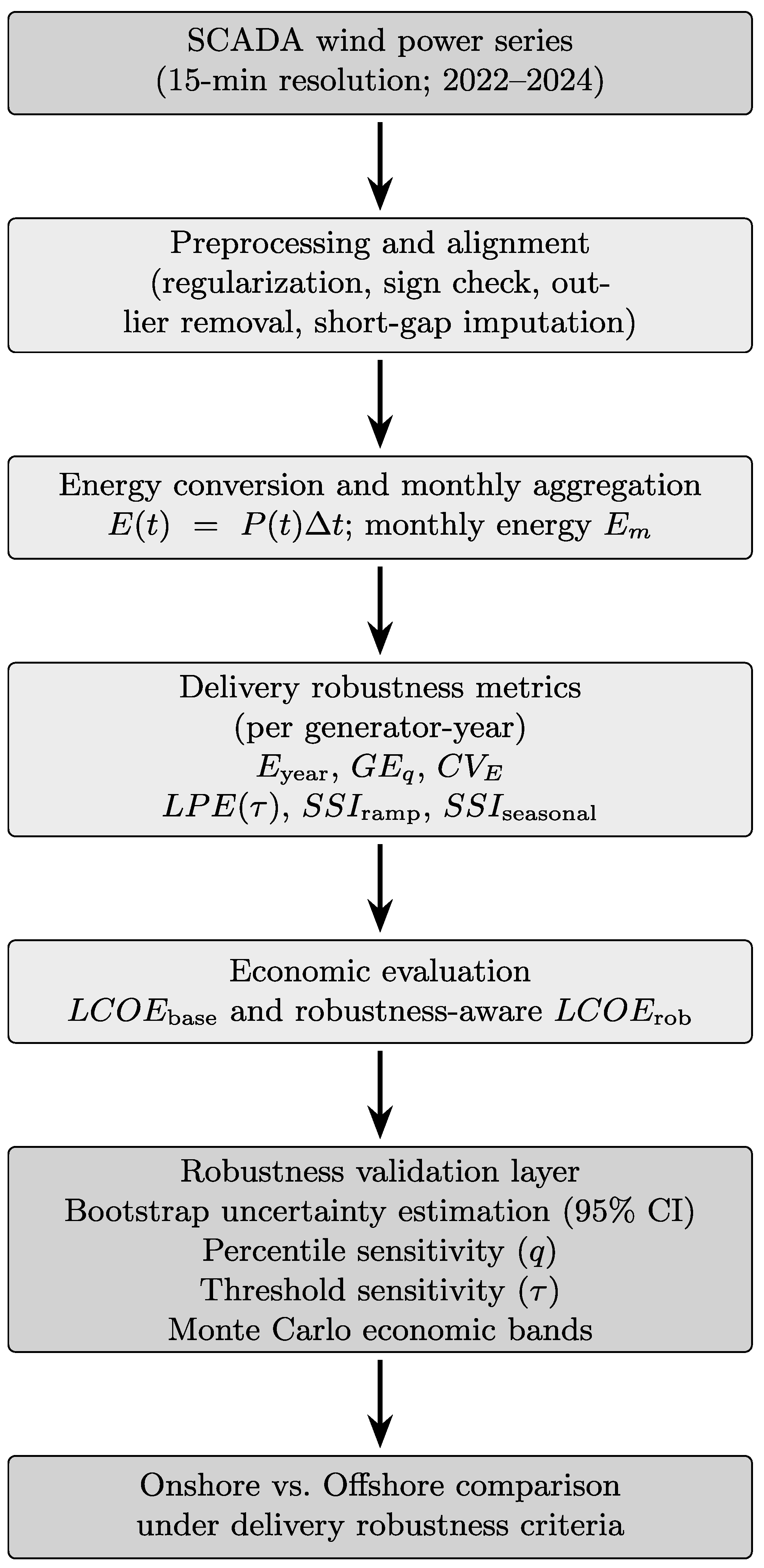
The remainder of the paper is organized as follows. Section 2 describes the dataset and preprocessing procedures. Section 3 introduces the delivery robustness indicators, the uncertainty and sensitivity analysis procedures, and the robustness-aware economic evaluation framework. Section 4 presents the empirical results obtained from the analyzed wind units, while Section 5 interprets the implications of delivery stability for techno-economic robustness. Finally, Section 6 summarizes the main findings and outlines directions for future research.

2. Data and Preprocessing

The present study builds upon the real 60 kV distribution network previously analyzed in [21], where the structural and contingency-related impacts of integrating wind generation were investigated. In contrast to that work, which focused on network-level operational effects, the current study evaluates delivery robustness and economic sensitivity using the same high-resolution operational dataset.

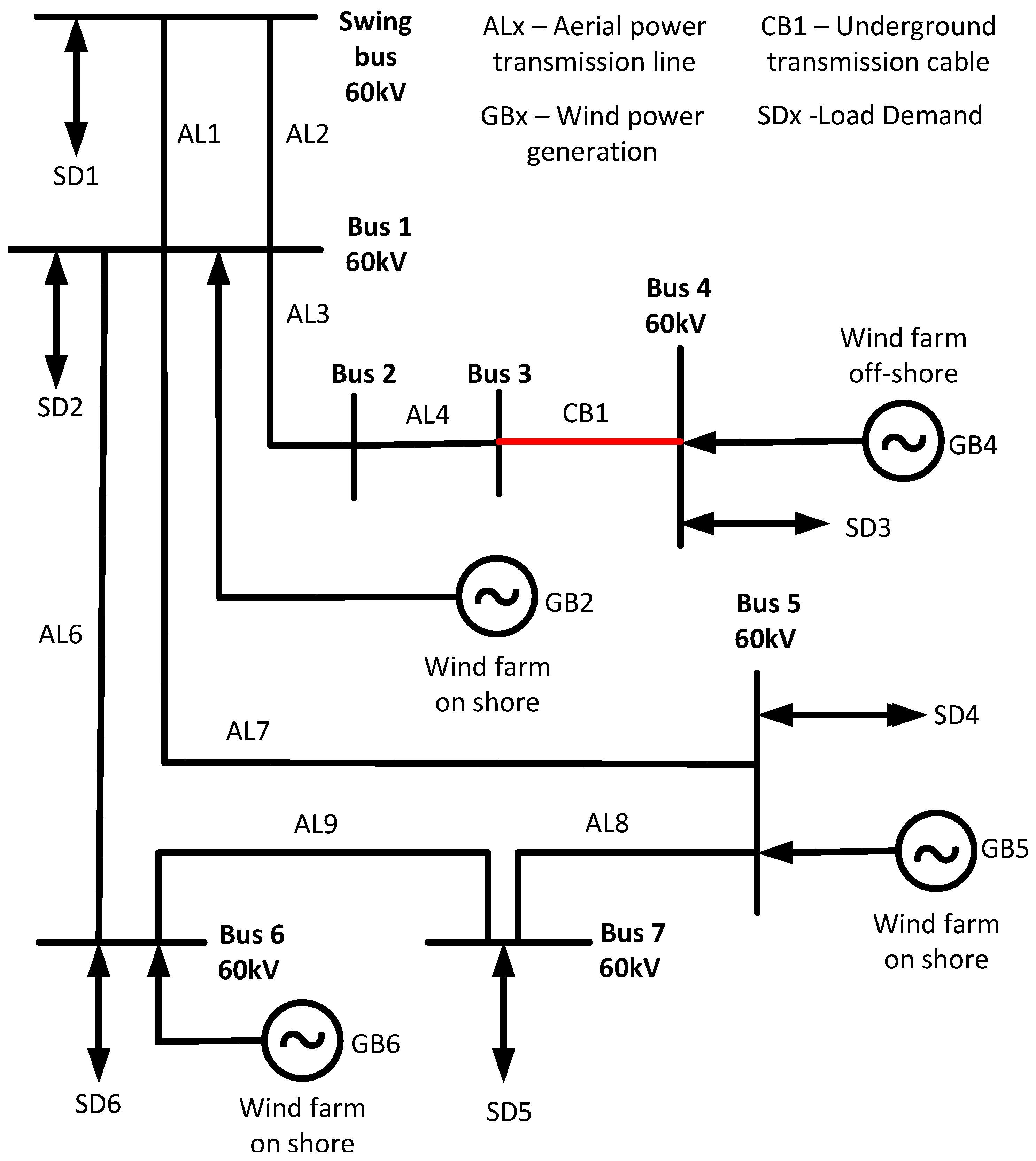
For contextual completeness, the network topology and geographic positioning of the analyzed wind units are reproduced in Figure 1. The system comprises one offshore wind farm (GB4) and three onshore wind farms (GB2, GB5, and GB6) connected to a real 60 kV distribution network. While the electrical configuration is retained for reference, the present analysis does not perform power flow or contingency simulations, focusing instead on statistical robustness indicators derived from measured production data.

2.1. Dataset Description

The study analyzes four utility-scale wind units located in Portugal, comprising three onshore units and one offshore unit. For confidentiality, units are anonymized as GB2–GB6, with GB4 corresponding to the offshore installation. Given the limited sample size, especially the availability of a single offshore unit, the results are interpreted as a comparative case study within the analyzed dataset rather than as a universally generalizable characterization of all onshore and offshore wind assets.

Active power output was recorded at 15-min intervals over the period 2022–2024, resulting in more than 300,000 observations per unit (approximately 35,000 measurements per year). This high temporal resolution allows statistically robust estimation of monthly energy delivery and variability indicators.

The analysis is conducted at unit level. Network topology, curtailment mechanisms, and market participation rules are not explicitly modeled in order to isolate intrinsic delivery behavior. This choice allows the comparison to focus on temporal delivery characteristics rather than on network-constrained dispatch outcomes.

2.2. Data Cleaning and Alignment

Time stamps were sorted and aligned to a regular 15-min grid. Duplicate entries were removed. An automatic sign verification ensured consistent generation convention; if the median power was negative, the series was inverted.

Non-physical values and negative outputs were excluded. When nominal rated power values were unavailable due to data-access and confidentiality constraints associated with the proprietary SCADA dataset, a proxy rated value was estimated as the 99th percentile of observed power. This proxy was used exclusively for signal normalization and plausibility screening, rather than as a direct techno-economic input. Measurements exceeding 1.10 times the rated (or proxy-rated) power were treated as implausible and removed.

Short data gaps up to 60 min were linearly interpolated to preserve aggregation consistency. After preprocessing, missing values were negligible and did not affect monthly aggregation.

2.3. Energy Aggregation

Energy delivered at time step t is computed as

$$E\left(t\right)=P\left(t\right)\Delta t,$$

(1)

with $\Delta t=0.25$ h corresponding to the 15-min SCADA sampling interval.

Monthly delivered energy values $\left\{E_m\right\}$ are obtained by summing $E\left(t\right)$ within each calendar month. Monthly aggregation provides a practical compromise between short-term fluctuation smoothing and preservation of medium-term variability relevant for robustness assessment.

3. Methods

3.1. Energy Delivery Robustness Metrics

Robustness is evaluated through complementary indicators derived from monthly energy $\left\{E_m\right\}$ and normalized power $p\left(t\right)=P\left(t\right)/P_{\mathrm{rated}}$. Several indicators follow standard statistical variability analysis and resource adequacy metrics commonly adopted in wind power integration studies [7,8,9], while two indices are introduced here to characterize operational smoothness and seasonal delivery balance: $SS{I}_{\mathrm{ramp}}$ and $SS{I}_{\mathrm{seasonal}}$. These two indices are not intended as universal standards, but as compact normalized descriptors tailored to the present delivery-oriented analysis. The ramp-based index emphasizes typical short-term operational smoothness through the median absolute power increment, which is less sensitive to isolated extreme events than the mean. The seasonal index measures how close the weakest quarterly delivery level remains to the overall monthly average, thereby capturing seasonal imbalance in a conservative and easily interpretable form.

Together, these indicators define a delivery-oriented evaluation framework designed to assess the robustness of wind energy supply under temporal variability and conservative energy assumptions. This set of metrics can be viewed as a delivery robustness assessment framework (DRAF), linking statistical variability indicators, conservative energy delivery proxies, and robustness-adjusted economic performance metrics. Within this framework, variability indicators characterize temporal dispersion and low-production exposure, delivery metrics quantify conservative energy availability, and economic indicators evaluate the resulting techno-economic sensitivity.

3.1.1. Annual Delivered Energy

$$E_{\mathrm{year}}=\sum _{m=1}^{12}{E}_m.$$

(2)

3.1.2. Guaranteed Monthly Energy

$$G{E}_q=Q_q\left(\left\{E_m\right\}\right),$$

(3)

where $Q_q(·)$ denotes the empirical q-th percentile of the monthly energy distribution, with baseline value $q=10$. This percentile-based indicator represents a conservative proxy of monthly energy delivery and is used to derive robustness-aware annual energy in the subsequent economic assessment.

Percentile-based metrics are commonly used to evaluate conservative energy availability and adequacy contributions of wind generation [8,16].

3.1.3. Dispersion of Monthly Delivery

$$C{V}_E={\displaystyle \frac{\sigma \left(E_m\right)}{\mu \left(E_m\right)}}.$$

(4)

The coefficient of variation is widely used to quantify variability in renewable generation datasets and power system integration studies [7,9].

3.1.4. Low-Production Exposure

$$LPE\left(\tau \right)={\displaystyle \frac{1}{T}}\sum _{t=1}^T\mathbb{I}(p\left(t\right)<\tau ),$$

(5)

with $\tau \in \{0.20,0.25,0.30\}$. For the baseline comparison reported in

Table 1. Annual delivery robustness and economic performance metrics for each unit over the 2022–2024 period. The table summarizes expected annual energy, guaranteed energy, variability indicators, and robustness-aware economic metrics. The tail robustness ratio $T{R}_{10}$ quantifies the proportion of annual energy preserved under conservative lower-tail delivery assumptions. Low-production exposure is reported for $\tau =0.25$. The amplification factor $AF=LCO{E}_{\mathrm{rob}}/LCO{E}_{\mathrm{base}}$ quantifies the economic sensitivity to conservative delivery assumptions and represents the relative cost amplification associated with variability-driven reductions in guaranteed energy.

Unit	Group	Year	${\mathit{E}}_{\mathbf{year}}$	${\mathit{GE}}_{10}$	${\overline{\mathit{E}}}_{\mathit{m}}$	${\mathit{CV}}_{\mathit{E}}$	${\mathit{LPE}}_{0.25}$	${\mathit{SSI}}_{\mathbf{ramp}}$	${\mathit{SSI}}_{\mathbf{seasonal}}$	${\mathit{TR}}_{10}$	${\mathit{LCOE}}_{\mathbf{base}}$	${\mathit{LCOE}}_{\mathbf{rob}}$	$\mathit{AF}$
			(GWh)	(GWh)	(GWh)						(EUR/MWh)	(EUR/MWh)
GB2	Onshore	2022	85.48	3.94	7.12	0.360	0.606	0.987	0.709	0.55	84.68	1836.48	21.69
GB2	Onshore	2023	87.23	4.50	7.27	0.306	0.585	0.986	0.736	0.62	82.98	1609.54	19.40
GB2	Onshore	2024	91.79	4.32	7.65	0.258	0.553	0.984	0.777	0.56	78.85	1673.94	21.23
GB4	Offshore	2022	78.14	4.75	6.51	0.204	0.552	0.988	0.861	0.73	88.93	1463.71	16.46
GB4	Offshore	2023	79.16	4.06	6.60	0.268	0.531	0.991	0.800	0.62	87.78	1711.77	19.50
GB4	Offshore	2024	85.96	4.08	7.16	0.293	0.496	0.990	0.744	0.57	80.84	1702.61	21.06
GB5	Onshore	2022	95.77	3.54	7.98	0.417	0.586	0.988	0.666	0.44	71.95	1945.44	27.04
GB5	Onshore	2023	104.56	4.40	8.71	0.407	0.563	0.988	0.674	0.50	65.90	1567.28	23.78
GB5	Onshore	2024	104.71	4.12	8.73	0.355	0.541	0.986	0.646	0.47	65.81	1673.27	25.43
GB6	Onshore	2022	23.94	1.01	1.99	0.485	0.651	0.987	0.729	0.51	82.25	1945.86	23.66
GB6	Onshore	2023	28.65	1.27	2.39	0.412	0.585	0.984	0.699	0.53	68.71	1551.21	22.57
GB6	Onshore	2024	28.85	1.33	2.40	0.309	0.558	0.981	0.683	0.55	68.24	1485.44	21.77

, $\tau =0.25$ is adopted.

Indicators based on low-production thresholds are frequently used to characterize the adequacy contribution and variability exposure of wind generation resources [9].

3.1.5. Operational Stability Index

$$SS{I}_{\mathrm{ramp}}=1-{\displaystyle \frac{{\mathrm{median}}_t\left(|\Delta P(t\left)\right|\right)}{P_{\mathrm{rated}}}},$$

(6)

where $\Delta P\left(t\right)=P\left(t\right)-P(t-1)$ represents the power ramp between consecutive time steps. The median operator is used to characterize the typical magnitude of short-term ramps while limiting the influence of isolated extremes or transient measurement anomalies. Normalization by $P_{\mathrm{rated}}$ makes the index dimensionless and comparable across units of different nominal capacities. The index is bounded to the interval [0,1], with higher values indicating smoother operational behavior and lower typical ramp variability relative to rated capacity.

3.1.6. Seasonal Stability

To avoid ambiguity with the percentile level q, quarterly seasons are indexed by $k\in \{1,2,3,4\}$, and the seasonal stability index is defined as

$$SS{I}_{\mathrm{seasonal}}={\displaystyle \frac{{min}_{k\in \{1,2,3,4\}}{\overline{E}}^{\left(k\right)}}{\mu \left(E_m\right)}},$$

(7)

where ${\overline{E}}^{\left(k\right)}$ denotes the mean monthly energy within quarter k. This indicator quantifies seasonal delivery balance by comparing the weakest quarterly mean with the overall mean monthly production. By construction, it emphasizes the most adverse seasonal regime and therefore acts as a conservative indicator of seasonal asymmetry. Higher values indicate more uniform seasonal energy distribution.

3.1.7. Tail Robustness Ratio

To characterize the relationship between expected and conservative delivery, a tail robustness ratio is defined:

$$T{R}_q={\displaystyle \frac{12·G{E}_q}{E_{\mathrm{year}}}}.$$

(8)

Higher $T{R}_q$ values indicate that lower-tail delivery remains proportionally closer to the expected annual energy, reflecting stronger delivery robustness. When full annual data are available ($n_M=12$), the robustness-aware annual energy becomes $E_{\mathrm{rob}}=12G{E}_q$, and therefore the tail robustness ratio can be interpreted as the ratio between conservative and expected annual energy, i.e., $T{R}_q=E_{\mathrm{rob}}/E_{\mathrm{year}}$.

This indicator is conceptually related to percentile-based energy adequacy metrics used in wind generation reliability studies [8].

3.2. Economic Assessment

The Levelized Cost of Energy formulation follows standard definitions used in renewable energy economic assessments. Baseline LCOE is defined as

$$LCO{E}_{\mathrm{base}}={\displaystyle \frac{CAPEX+{\sum }_{t=1}^{T_p}\frac{O\&M}{{(1+r)}^t}}{{\sum }_{t=1}^{T_p}\frac{E_{\mathrm{year}}}{{(1+r)}^t}}},$$

(9)

where $T_p$ denotes the project lifetime in years.

This formulation is widely adopted in energy technology cost comparisons [1,2].

Robustness-aware annual energy is obtained by annualizing guaranteed monthly energy:

$$E_{\mathrm{rob}}=G{E}_q·{\displaystyle \frac{12}{n_M}},$$

(10)

where $n_M$ is the number of available months in the considered year (typically $n_M=12$ after preprocessing).

Robustness-aware LCOE is therefore

$$LCO{E}_{\mathrm{rob}}={\displaystyle \frac{CAPEX+{\sum }_{t=1}^{T_p}\frac{O\&M}{{(1+r)}^t}}{{\sum }_{t=1}^{T_p}\frac{E_{\mathrm{rob}}}{{(1+r)}^t}}}.$$

(11)

It is important to emphasize that $LCO{E}_{\mathrm{rob}}$ should not be interpreted as a market cost of electricity or as a conventional project appraisal metric. Instead, it represents a conservative robustness-aware indicator obtained by replacing expected annual energy with a lower-tail delivery proxy derived from guaranteed monthly energy. Because guaranteed energy values are intentionally conservative and may represent a substantially reduced effective energy basis, $LCO{E}_{\mathrm{rob}}$ can reach numerical levels well above conventional $LCO{E}_{\mathrm{base}}$ estimates. In this sense, the metric is designed for comparative robustness assessment rather than absolute cost estimation. Its main purpose is to quantify relative cost amplification under conservative delivery assumptions and thereby support risk-aware ranking between assets with different temporal stability characteristics.

3.3. Uncertainty and Sensitivity

Month-level bootstrap resampling (2000 draws) is applied to the aggregated monthly energy values within each unit-year. For each bootstrap replicate, the available monthly observations are resampled with replacement while preserving the original sample size, and the corresponding robustness and economic indicators are recomputed. The resulting empirical distributions are used to estimate 95% confidence intervals for $G{E}_q$, $C{V}_E$, $SS{I}_{\mathrm{seasonal}}$, and $LCO{E}_{\mathrm{rob}}$.

Sensitivity analyses evaluate the robustness of the proposed indicators with respect to methodological and economic assumptions:

• Variation in percentile $q\in \{5,10,20\}$;
• Variation in threshold $\tau \in \{0.20,0.25,0.30\}$;
• Monte Carlo variation in economic parameters (CAPEX multiplier, O&M fraction, discount rate).

In the Monte Carlo analysis, CAPEX multiplier, O&M fraction, and discount rate are independently sampled within the prescribed ranges in order to propagate parameter uncertainty into $LCO{E}_{\mathrm{rob}}$. This stochastic sampling approach allows the sensitivity of the robustness-aware economic indicator to realistic variations in techno-economic inputs to be evaluated [23].

As a complementary validation step, Spearman rank correlation analysis was performed between the proposed stability indicators and reference variability/robustness metrics. Spearman correlation was selected because it is appropriate for small samples and evaluates monotonic associations without assuming linearity or normality of the variables [24].

3.4. Workflow Summary and Implementation Outline

To enhance reproducibility and provide a compact overview of the methodological pipeline, Figure 2 presents the workflow from SCADA data ingestion to the robustness-validation layer (bootstrap uncertainty, parametric sensitivity, and Monte Carlo economic bands). The computational steps implemented to generate the reported metrics are summarized below. The main computational steps are summarized in Algorithm 1.

Algorithm 1: Robustness-informed techno-economic pipeline

1. Input: SCADA power series $P_g\left(t\right)$ (15-min resolution), percentile level q, threshold $\tau$, and economic parameters $(CAPEX,O\&M,r)$. 2. Preprocessing and alignment (a) Regularize timestamps to a uniform 15-min grid and remove duplicates. (b) Verify generation sign convention and correct if necessary. (c) Remove negative or non-physical values. (d) Estimate rated power $P_{\mathrm{rated}}$ (e.g., p99 proxy if unavailable). (e) Clip values exceeding $1.10P_{\mathrm{rated}}$. (f) Interpolate short gaps (up to 60 min). 3. Energy conversion and aggregation (a) Compute step energy: $E\left(t\right)=P\left(t\right)\Delta t$. (b) Aggregate monthly energy values $E_m$. 4. Yearly robustness metrics (per unit-year) (a) Compute annual delivered energy $E_{\mathrm{year}}$. (b) Compute guaranteed energy $G{E}_q$. (c) Compute dispersion coefficient $C{V}_E$. (d) Compute low-production exposure $LPE\left(\tau \right)$. (e) Compute $SS{I}_{\mathrm{ramp}}$ and $SS{I}_{\mathrm{seasonal}}$. (f) Compute tail robustness ratio $T{R}_q$. 5. Economic evaluation (a) Compute baseline $LCO{E}_{\mathrm{base}}$. (b) Compute robustness-aware annual energy $E_{\mathrm{rob}}$. (c) Compute robustness-aware $LCO{E}_{\mathrm{rob}}$. 6. Robustness validation (a) Apply month-level bootstrap (95% confidence intervals). (b) Evaluate sensitivity to percentile q. (c) Evaluate sensitivity to threshold $\tau$. (d) Perform Monte Carlo simulation for economic parameters. 7. Output: Tables and figures supporting onshore vs. offshore comparison.

4. Results

4.1. Monthly Energy Distribution

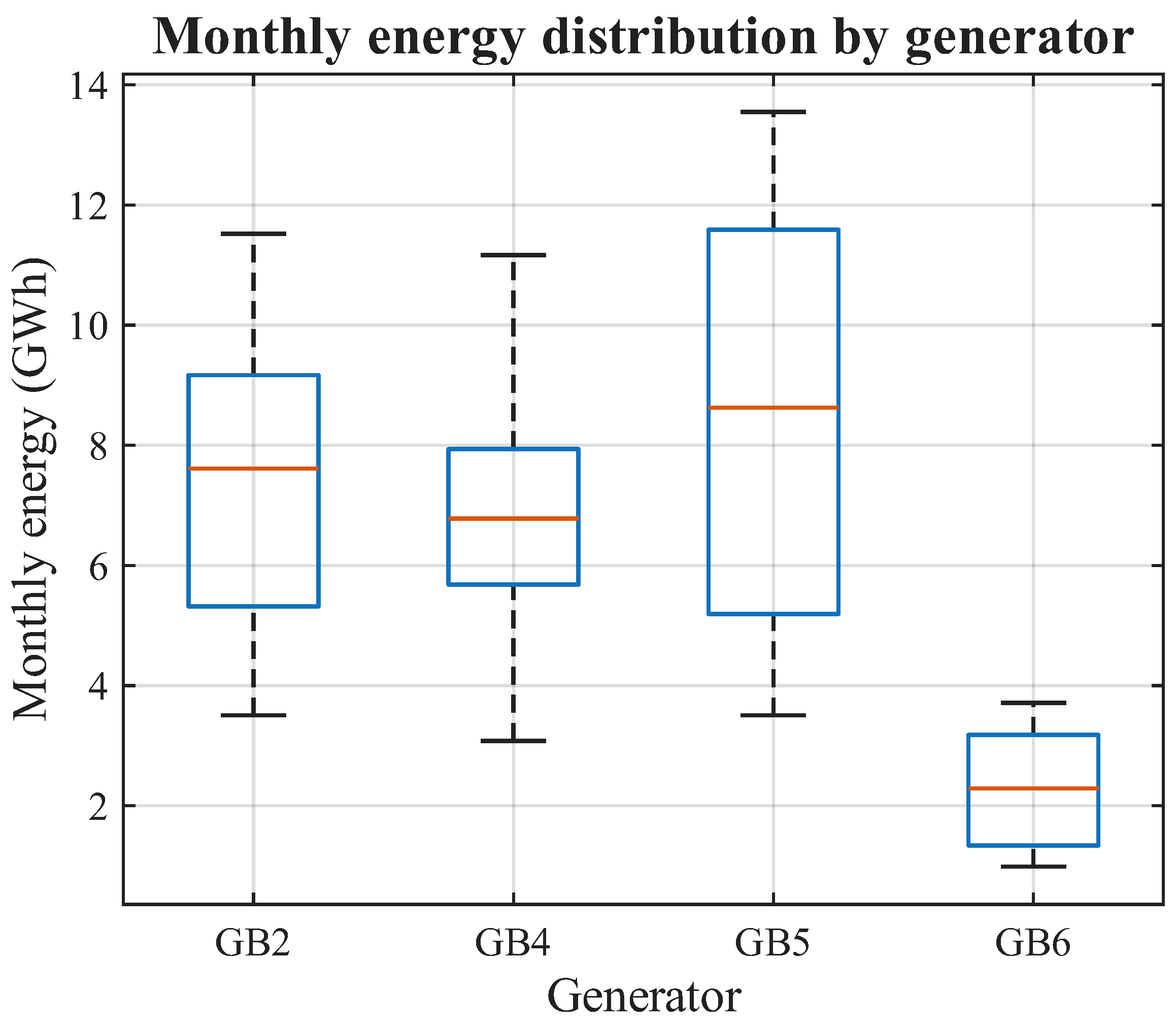
Figure 3 shows the distribution of monthly delivered energy for all units over 2022–2024. The offshore unit exhibits a visibly narrower interquartile range and fewer pronounced low-tail months compared to the onshore units, indicating tighter monthly dispersion and improved delivery regularity across years. These structural differences are reflected quantitatively in the annual dispersion metrics summarized in Table 1, where the analyzed offshore unit systematically attains lower $C{V}_E$ values than its onshore counterparts.

Taken together, the boxplots and dispersion indicators suggest that the analyzed offshore unit maintains a more stable monthly delivery profile than the analyzed onshore units within the same regional context. This pattern is consistent with the smoother and more persistent offshore conditions previously identified through entropy-based uncertainty metrics in [21].

Table 1 reveals a clear structural contrast between offshore and onshore energy delivery. Among the reported indicators, $T{R}_{10}$ and $AF$ are especially useful for summarizing the link between conservative delivery robustness and economic sensitivity. The tail robustness ratio $T{R}_{10}$ further clarifies the relationship between expected and conservative energy delivery. Higher values of $T{R}_{10}$ indicate that guaranteed monthly energy remains closer to the expected annual production, reflecting stronger lower-tail delivery stability. As a consequence, units with higher $T{R}_{10}$ values experience smaller reductions in robustness-aware annual energy $E_{\mathrm{rob}}$, which directly mitigates the amplification observed in $LCO{E}_{\mathrm{rob}}$. This relationship helps explain why the analyzed offshore unit systematically exhibits lower economic amplification under conservative delivery assumptions.

It should be noted that GB6 exhibits substantially lower annual delivered energy than the other analyzed units. This difference is associated with the specific scale and operating profile of that unit and does not, by itself, invalidate the comparative robustness analysis, since the main indicators discussed in this study are based on normalized or relative measures of delivery behavior, including monthly dispersion ($C{V}_E$), low-production exposure ($LPE$), stability indices, tail robustness ratio ($T{R}_{10}$), and amplification factor ($AF$). Accordingly, the comparison focuses on temporal delivery characteristics and robustness patterns rather than on absolute production totals alone.

Across all three years, the analyzed offshore unit (GB4) consistently demonstrates lower monthly dispersion ($C{V}_E$), reduced low-production exposure, and higher seasonal stability relative to the onshore units. While absolute annual energy values are of comparable magnitude, the guaranteed energy metric ($G{E}_{10}$) remains systematically closer to the annual mean in the offshore case, indicating a tighter lower-tail distribution and stronger delivery robustness. This structural advantage translates into economic resilience: the amplification from $LCO{E}_{\mathrm{base}}$ to $LCO{E}_{\mathrm{rob}}$ is consistently lower for the offshore unit, confirming that delivery stability mitigates variability-driven cost escalation under conservative energy assumptions.

4.2. Robustness Indicators

Table 1 shows that the analyzed offshore unit consistently exhibits lower monthly dispersion. Averaged over 2022–2024, the coefficient of variation is 0.255 for the offshore unit compared to 0.368 for onshore units, corresponding to an approximate 30% reduction in relative variability.

Low-production exposure follows the same structural pattern. The offshore unit records an average $LPE$ of 0.526, while onshore units reach 0.581, indicating systematically reduced time spent below the defined low-production threshold. For consistency with the baseline robustness comparison, Table 1 reports the indicator evaluated at $\tau =0.25$, while additional threshold levels are examined in the sensitivity analysis.

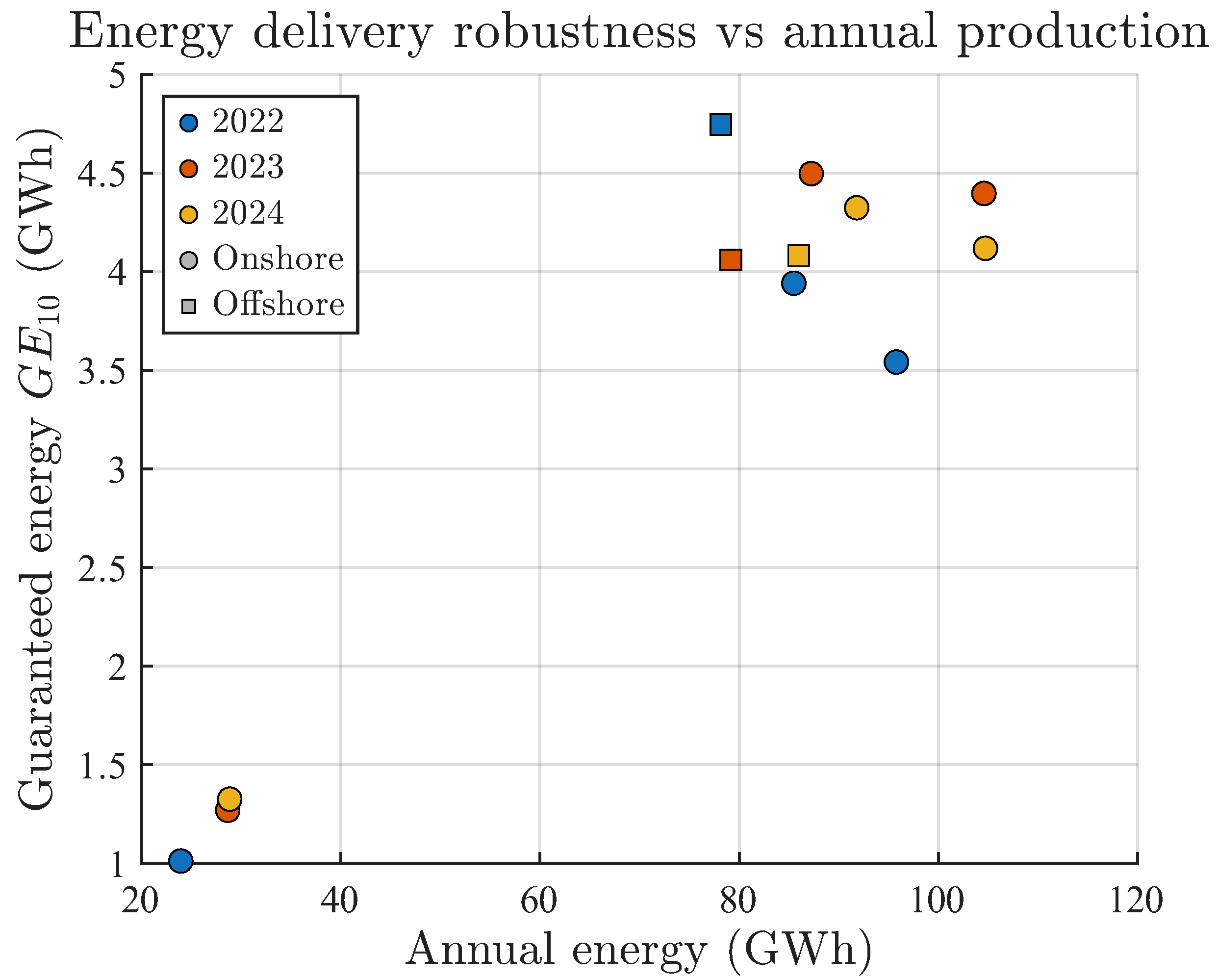
Figure 4 illustrates the relationship between annual energy and guaranteed delivery ($G{E}_{10}$). The analyzed offshore unit tends to retain comparatively higher guaranteed monthly energy relative to its annual production level than the analyzed onshore units, indicating improved lower-bound delivery reliability.

To further interpret the relationship between expected and conservative delivery, the tail robustness ratio $T{R}_{10}$ was evaluated. Across the analyzed years, the offshore unit exhibits consistently higher $T{R}_{10}$ values compared with the onshore units, indicating that guaranteed delivery remains proportionally closer to expected annual production. This confirms that offshore generation not only reduces dispersion but also improves lower-bound delivery reliability. This helps explain the lower robustness-induced cost amplification observed for offshore generation in the economic analysis.

4.3. Economic Comparison

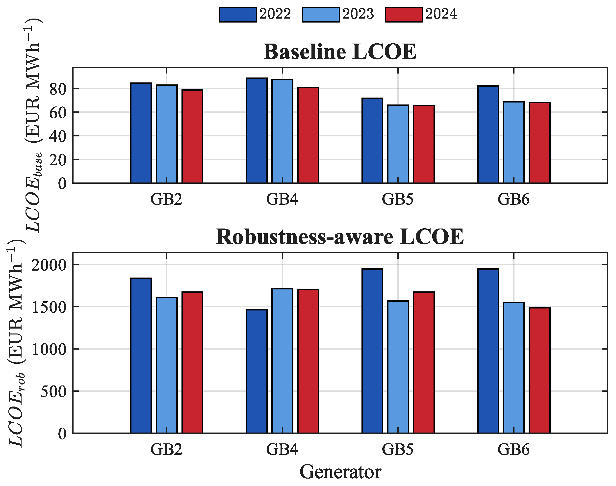
Figure 5 illustrates the economic implications of delivery robustness. All units experience cost amplification when conservative energy assumptions are introduced; however, the magnitude of this amplification differs. The analyzed offshore unit exhibits consistently lower relative escalation from $LCO{E}_{\mathrm{base}}$ to $LCO{E}_{\mathrm{rob}}$, evidencing that structural delivery stability mitigates variability-driven cost penalties. These values should be interpreted as robustness-sensitive comparative indicators rather than as direct estimates of market electricity cost, since the conservative annual energy basis used in $LCO{E}_{\mathrm{rob}}$ intentionally magnifies the economic effect of lower-tail delivery behavior.

Because the robustness-aware annual energy $E_{\mathrm{rob}}$ is derived from guaranteed monthly energy ($G{E}_q$), lower delivery stability directly reduces the effective energy considered in the economic model. Consequently, units with higher variability experience a stronger increase in $LCO{E}_{\mathrm{rob}}$.

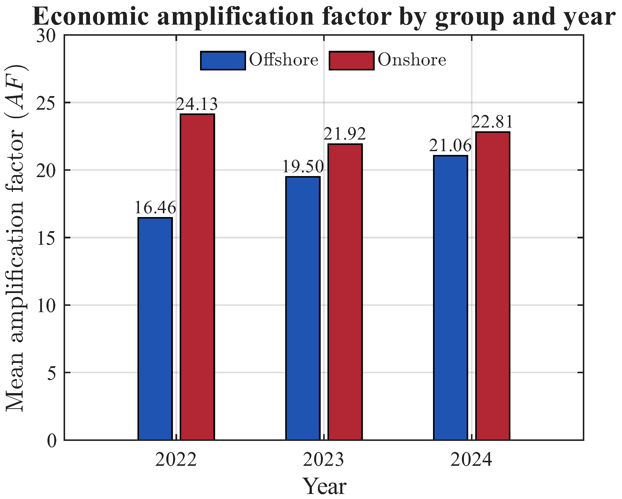
To make this effect explicit, the amplification factor is defined as:

$$AF={\displaystyle \frac{LCO{E}_{\mathrm{rob}}}{LCO{E}_{\mathrm{base}}}}.$$

(12)

The amplification factor $AF$ provides a compact indicator of the economic impact of delivery variability, capturing how reductions in guaranteed energy propagate into robustness-adjusted cost metrics. Higher $AF$ values indicate stronger cost escalation when conservative delivery assumptions are adopted and therefore reflect the economic sensitivity of wind generation assets to lower-tail production behavior.

Across 2022–2024, the mean $AF$ is lower for offshore than for onshore units, indicating reduced economic sensitivity to adverse delivery tails, as illustrated in Figure 6.

4.4. Uncertainty and Sensitivity Analysis

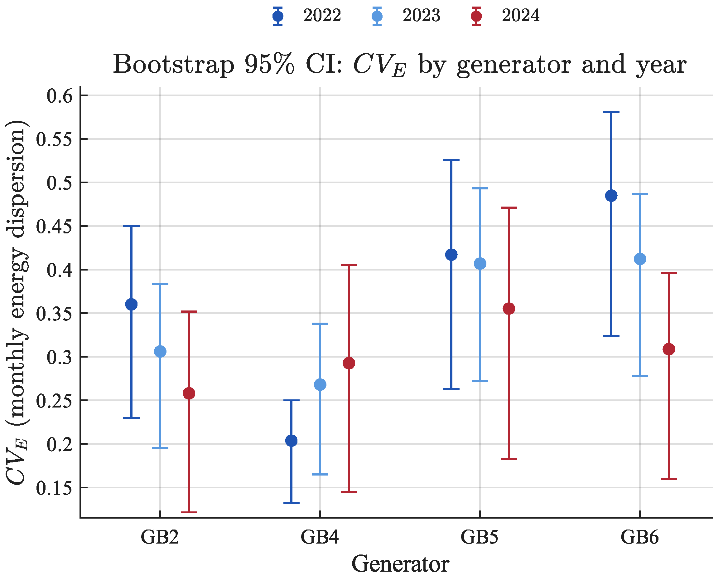
Bootstrap confidence intervals presented in Figure 7 reinforce the structural contrast in monthly dispersion. Although uncertainty bands overlap across units, the analyzed offshore unit systematically occupies a lower and more compact interval range, indicating reduced uncertainty and lower values of $C{V}_E$ relative to the analyzed onshore units.

Overall, these results confirm that the onshore–offshore contrast is not parameter-dependent and that the group ranking remains unchanged.

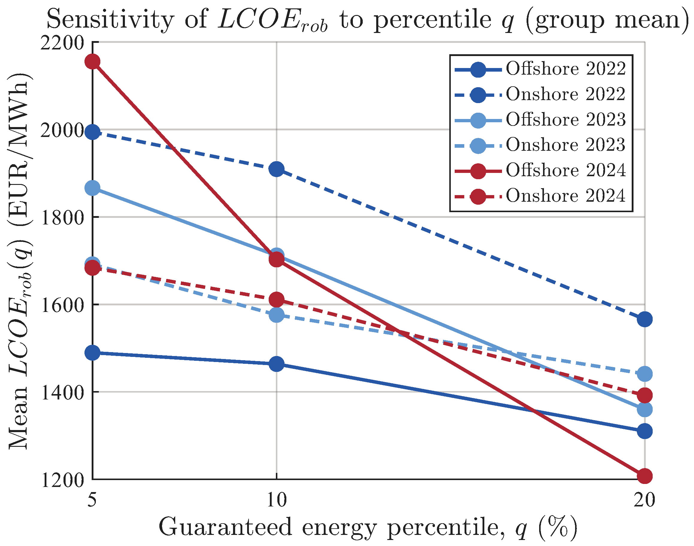
The sensitivity analysis in Figure 8 confirms that the observed onshore–offshore ranking remains unchanged across percentile levels ranging from 5% to 20%. The analyzed offshore unit maintains lower robustness-adjusted cost levels and a flatter sensitivity slope, indicating that the robustness conclusions do not depend on a specific percentile selection.

Collectively, the evidence indicates that the analyzed offshore unit exhibits superior delivery robustness relative to the analyzed onshore units across dispersion, lower-tail reliability, and variability-adjusted economic performance. This structural advantage is consistent across years, statistically supported, and remains stable under percentile selection, indicating that the observed contrast appears robust to the tested methodological choices and is unlikely to be explained solely by parameter selection.

5. Discussion

This study extends baseline comparisons between onshore and offshore wind generation by evaluating the robustness of delivery-oriented performance metrics under parametric and economic uncertainty. Rather than reassessing absolute performance levels, the analysis focused on the consistency of the offshore–onshore contrast when key assumptions are varied. The results also illustrate how the proposed delivery robustness assessment framework (DRAF) provides a structured way to connect variability indicators, conservative energy delivery metrics, and economic performance measures.

5.1. Robustness of Delivery Metrics

The sensitivity analyses indicate that variations in percentile definitions and low-production thresholds affect absolute metric values but do not substantially modify the relative positioning between offshore and onshore units. Across the tested parameter ranges, the analyzed offshore unit consistently exhibits lower dispersion and reduced exposure to low-production regimes.

These findings suggest that the previously observed offshore advantage is not strongly dependent on a specific percentile or threshold choice. Instead, it appears associated with underlying temporal characteristics of the wind regime, particularly smoother monthly distribution and reduced variability concentration.

To further support the interpretation of the proposed stability indices, a complementary Spearman correlation analysis was performed between the proposed indicators and more conventional variability and robustness measures. The seasonal stability index showed a strong positive association with the tail robustness ratio and a strong negative association with the monthly energy dispersion coefficient, supporting its interpretation as a compact descriptor of seasonal delivery balance. In contrast, the ramp-based stability index exhibited weaker associations with aggregated annual variability measures, suggesting that it captures short-term operational smoothness that is not fully reflected by broader monthly delivery indicators. Taken together, the correlations reported in the Supplementary Materials, Section S4, support the interpretation of $SS{I}_{\mathrm{seasonal}}$ as a compact descriptor of seasonal delivery robustness, while suggesting that $SS{I}_{\mathrm{ramp}}$ reflects a distinct short-term operational dimension that is not strongly captured by aggregated annual variability metrics.

A complementary perspective emerges from the joint behavior of the variability and robustness indicators. The analyzed offshore unit consistently exhibits both lower monthly dispersion ($C{V}_E$) and higher tail robustness ratios ($T{R}_{10}$) compared with the onshore units. This combination indicates that offshore wind production not only reduces variability but also preserves a larger fraction of annual energy under conservative delivery assumptions. As a consequence, the robustness-aware annual energy remains closer to the expected production level, which ultimately moderates the amplification observed in $LCO{E}_{\mathrm{rob}}$.

5.2. Economic Behavior Under Stochastic Inputs

Previous studies have also shown that temporal variability in wind resources can significantly influence economic indicators such as the Levelized Cost of Energy, particularly when variability reduces the effective energy available under conservative assumptions [19].

A clearer interpretation of the observed economic behavior emerges when the interaction between the variability and robustness indicators is considered jointly. Units with higher monthly dispersion ($C{V}_E$) tend to experience greater exposure to low-production regimes ($LPE$), which in turn reduces the guaranteed monthly energy $G{E}_q$. This reduction directly decreases the robustness-aware annual energy $E_{\mathrm{rob}}$, thereby amplifying the robustness-adjusted cost metric $LCO{E}_{\mathrm{rob}}$. In contrast, units characterized by smoother production profiles exhibit lower variability, reduced exposure to low-production periods, and higher tail robustness ratios ($T{R}_q$). This chain of effects helps explain why the analyzed offshore unit experiences systematically lower economic amplification when conservative delivery assumptions are applied.

Monte Carlo simulations incorporating variability in CAPEX, O&M costs, and discount rates further indicate that the offshore–onshore ranking remains stable under stochastic economic assumptions. While the offshore unit retains higher capital expenditure, improved delivery stability partially offsets variability-driven cost amplification when conservative delivery assumptions are considered.

These results should nevertheless be interpreted within the scope of the present economic formulation, which does not explicitly model market-based mechanisms such as imbalance penalties, revenue volatility, or delivery-linked financing conditions. In real-world electricity markets, such mechanisms could further increase the economic relevance of lower-tail delivery stability, particularly for assets exposed to production shortfalls, balancing costs, or contract structures sensitive to delivery regularity.

5.3. Implications for Investment and Planning

In renewable-dominated systems, investment decisions increasingly require risk-aware performance evaluation. The integration of percentile-based delivery indicators and stochastic economic modeling provides a more nuanced understanding of techno-economic sensitivity.

From a planning perspective, improved temporal stability may partially offset higher upfront investment, particularly in contexts where variability-related penalties or conservative financing assumptions are relevant. The results support the view that temporal regularity constitutes an economically relevant attribute.

This interpretation also suggests a natural extension of the framework to hybrid renewable systems with storage. By smoothing short-term variability and shifting energy across time, storage may improve guaranteed delivery metrics, reduce exposure to low-production regimes, and mitigate the economic amplification associated with conservative delivery assumptions. Evaluating these effects in hybrid configurations constitutes an important direction for future work.

5.4. Limitations

The analysis is based on a limited number of units within a single regional context. Although robustness trends are consistent across the tested parameter ranges, broader datasets and additional geographical contexts would strengthen the generalizability of the results. Furthermore, explicit modeling of market penalties or forecast error structures could provide deeper insight into the financial implications of delivery variability. Accordingly, the present results should be interpreted as evidence of a robust contrast within the analyzed sample rather than as a universally generalizable characterization of all offshore and onshore wind assets.

In particular, the relative offshore–onshore contrast observed here may vary under different climatic regimes, since persistence, seasonal balance, and low-production exposure are shaped by regional meteorological conditions.

A key limitation is the sample size, particularly the availability of a single offshore unit and proprietary data constraints limiting access to additional units within this 60 kV network. Nevertheless, the high temporal resolution of the dataset (>300,000 SCADA observations per unit, 15-min intervals over 2022–2024), combined with rigorous uncertainty quantification, month-level bootstrap resampling (2000 draws) and Monte Carlo simulation of economic parameters, supports the robustness of the observed onshore–offshore contrasts across years and sensitivity ranges. In addition, the present dataset does not explicitly span a broad range of turbine technologies, maintenance schedules, or operating strategies. These factors may influence both short-term operational smoothness and longer-term delivery behavior, and therefore broader portfolios should be examined in future work to assess how such heterogeneity affects the robustness patterns identified here. Future work will extend the analysis to larger wind portfolios and multi-regional datasets in order to further assess the generalizability of the proposed framework.

While these limitations constrain the geographical scope of the present study, they do not affect the methodological validity of the proposed delivery robustness framework.

6. Conclusions

This study investigated the robustness of delivery-oriented performance metrics for onshore and offshore wind generation under parametric and economic uncertainty. The results consistently show that the analyzed offshore unit exhibits stronger delivery robustness than the analyzed onshore units within the considered dataset. Averaged over 2022–2024, the offshore unit exhibited a lower monthly energy dispersion coefficient ($C{V}_E=0.255$) than the onshore units ($C{V}_E=0.368$), corresponding to an approximate 30% reduction in relative variability, and lower mean low-production exposure ($LPE=0.526$ versus $0.581$).

The results show that the contrast between onshore and offshore units remains broadly consistent across the tested parameter ranges. Although absolute values change with percentile definitions, low-production thresholds, and economic assumptions, the relative positioning between units is preserved, indicating that the observed offshore advantage within the analyzed dataset is not an artefact of a particular modelling choice.

The findings further indicate that this advantage is closely linked to the temporal structure of energy delivery rather than to total annual energy production alone. The offshore unit systematically combines lower monthly dispersion, reduced exposure to low-production regimes, and higher tail robustness ratios. As a consequence, a larger fraction of annual production remains available under conservative delivery assumptions, which directly mitigates the amplification observed in robustness-adjusted economic metrics. At group level, the mean amplification factor $AF$ remained lower for offshore than for onshore units in all analyzed years (16.46 vs. 24.13 in 2022, 19.50 vs. 21.92 in 2023, and 21.06 vs. 22.81 in 2024).

From a techno-economic perspective, the results highlight the importance of considering temporal delivery characteristics when evaluating renewable generation assets. Variability-driven reductions in guaranteed energy propagate through robustness-aware annual energy calculations and ultimately influence the behavior of cost indicators such as the robustness-adjusted Levelized Cost of Energy. In this context, delivery stability emerges as a relevant attribute alongside capital expenditure in the economic assessment of wind projects.

Overall, the proposed framework provides a structured methodology for linking temporal variability, delivery robustness indicators, and techno-economic sensitivity. These conclusions should therefore be interpreted within the scope of the analyzed dataset. Future work may extend the proposed framework in three main directions: first, by testing its applicability across larger wind portfolios and multi-regional datasets characterized by different climatic regimes; second, by examining how hybrid renewable systems with storage modify delivery robustness and variability-driven cost amplification; and third, by incorporating electricity market mechanisms in which delivery variability affects revenue stability, financing conditions, and long-term investment risk in renewable-dominated power systems.