Article

Power Collection System Optimization for Floating Offshore Wind Farms Combined with Oil and Gas Platforms Considering Wake Effect

1
Baima Lake Laboratory Co., Ltd., Hangzhou 311100, China
2
College of Control Science and Engineering, Zhejiang University, Hangzhou 310027, China
*
Author to whom correspondence should be addressed.
Energies 2026, 19(9), 2041; https://doi.org/10.3390/en19092041
Submission received: 1 April 2026 / Revised: 20 April 2026 / Accepted: 21 April 2026 / Published: 23 April 2026
(This article belongs to the Special Issue Recent Innovations in Offshore Wind Energy)

Abstract

Given the energy-intensive operations and considerable carbon emissions of offshore oil and gas platforms (OOGPs) in deep-sea regions, adopting floating offshore wind farms (FOWFs) as power sources offers substantial benefits. However, the expenses associated with dynamic submarine cables constitute a substantial portion of the capital expenditure (CAPEX) for this hybrid system, highlighting the crucial need for optimization in the power collection system design. In this study, we present a mixed-integer quadratic programming (MIQP) model designed to reduce both the costs of investment and power losses associated with dynamic submarine cables, taking into account the influence of the wake effect in local wind conditions. Due to the complexity of this problem, we employ the Benders’ decomposition method to reformulate it into a master problem and a slave problem. Additionally, two valid inequalities are specifically incorporated into the master problem to accelerate the solution process. These constraints are derived from a heuristic combination of various cable connection configurations and a greedy-based spanning tree structure. Through multiple case studies, we first demonstrate the accuracy and rapid convergence of our method. Furthermore, we reveal that as the wind farm grows in size, the influence of the wake effect becomes increasingly pronounced.

1. Introduction

Wind power has become a crucial component of the global clean energy strategy to mitigate carbon emissions, especially offshore wind with its higher energy density and more consistent wind distribution, surpassing that of onshore wind power [1]. In 2023, global wind power capacity grew by 116.6 GW, including 10.8 GW of offshore wind power [2], with expectations for continued global expansion driven by technological advancements [3]. Currently, most offshore wind turbines (OWTs) use bottom-fixed foundations in shallow water sites, typically no deeper than 60 m [1]. Conversely, floating offshore wind turbines (FOWTs) using floating platforms are not constrained by seabed conditions, making them ideal for deployment in deep-water areas where fixed-foundation turbines are impractical, especially in regions rich in offshore wind but lacking shallow water sites [4].
The potential synergy between FOWFs and offshore O&G platforms (OOGPs) is crucial, particularly in countries that possess significant offshore fossil and wind resources, such as Norway, China, Brazil, and the United States [5,6]. OOGPs, with energy-intensive facilities, need electrical power ranging from 10 MW to several hundred MW, mainly using gas turbines and synchronous generators [7,8]. Unfortunately, these gas turbines suffer from low efficiency, significant CO2 emissions, and high monetary expenses due to taxation on pollution [9]. FOWFs can supply electricity and alleviate these issues by interconnecting with OOGPs, particularly in deep-water areas far from the continental coast. This synergy reduces fuel consumption, providing environmental and financial benefits for OOGPs, and reduces the design and construction costs, liberating space and reducing operational risks [10,11]. FOWFs benefit from this synergy as well, as their generated electricity can be utilized by nearby OOGPs, resulting in substantial savings related to the construction costs of offshore substations, high-voltage transmission submarine cables, and costs related to transmission power losses.
In the last decade, numerous studies have explored integrating OOGPs with offshore wind farms [9,12,13,14,15,16]. Topics covered include gas turbine and wind turbine operation strategies [12], transient voltage and frequency stability [7,9,13], reactive compensation control [14,15], and sensitivity analysis of transients in an islanded system [16]. These discussions have fostered collaboration between OOGPs and FOWFs. In November 2022, Norway celebrated the inauguration of the Hywind Tampen Wind Farm, marking a historic milestone as the world’s first FOWF to supply power to OOGPs. The project, with 88 MW capacity and 260–300 m water depth, is poised to fulfill 35% of the annual power requirements for 5 OOGPs and reduce 200,000 t of CO2 emissions and 1000 t of NOx emissions each year [17]. As highlighted in recent sustainability-oriented energy studies [18], the integration of floating offshore wind with existing offshore infrastructure represents a scalable pathway toward decarbonizing the offshore energy sector. In March 2023, the first deep-sea FOWT of China, “Fuyao,” began operating offshore and is expected to power OOGPs in the South China Sea [19].
Despite these benefits, the high levelized cost of energy (LCoE) for FOWFs hinders their development [20]. To increase competitiveness in the energy market, reducing the electrical system costs of offshore wind farms is essential, with cables constituting 15–30% of the total CAPEX [21]. The proportion is even higher for the FOWFs, due to the higher costs of dynamic submarine cable [1]. Hence, the considerable influence of cable connection layout on the design of FOWFs, coupled with the substantial cable costs, underscores the significance of the cable connection layout optimization problem (CCLOP). The objective of CCLOP is to optimize the cable investment cost and power losses cost by devising an optimal layout for cable connections and selecting suitable cable types [22].
The optimization methods for CCLOP can be broadly categorized into deterministic and metaheuristic methods. Classic deterministic optimization methods, like mixed-integer linear programming, have been applied in previous studies [23,24,25,26,27,28,29,30]. Typically, deterministic methods solve CCLOP as a minimum spanning tree, but due to its NP-hardness, the computational time increases significantly with problem size [23]. To enhance solver efficiency, various techniques have been proposed [23,26,27,28,29], such as ignoring power losses costs within cables [26], disregarding the random wind velocity and direction properties [27], determining the optimal cable type in advance [23,28], and reducing the feasible number of cables inputting a wind turbine to one [29]. The complexity of CCLOP has led researchers to explore heuristic methods like genetic algorithm (GA) [31,32,33], clustering-based algorithm [34], hybrid genetic and immune algorithm [35], particle swarm optimization (PSO) algorithm [36], and adaptive particle swarm optimization (APSO) algorithm [22,37]. The CCLOP for FOWFs was initially introduced in [1], proposing an adapted particle swarm optimization algorithm that yields a suboptimal solution within an acceptable timeframe. What’s more, recent works have addressed full-system LCOE optimization for floating offshore wind farms, yet they treat cable layout as one component among many [38,39,40]. The present study complements both streams by focusing specifically on wake-aware cable collection system optimization for FOWFs supplying OOGPs, where cable-related costs dominate electrical infrastructure expenses.
This paper assumes all power generated by FOWFs directly transfers to the independent electrical grid of OOGPs, eliminating the need for a costly floating offshore substation and long high-voltage cable for transmitting power to the onshore grid. The contributions of the paper are outlined as follows: (i) Accurate calculation of power losses under various wind scenarios with consideration of the wake effect and stochastic power output from FOWTs, and formulate this complex problem as a Mixed-Integer Quadratic Programming (MIQP) model; (ii) Introduction of a virtual root integrating OOGPs and FOWTs into a simplified spanning tree structure to facilitate connection point selection; (iii) Proposal of two valid inequalities to expedite Benders’ decomposition in the cable routing optimization process, based on a greedy-based spanning tree structure and a heuristic hybridization process that incorporates different cable connection layouts.
This article is structured as follows: Section 2 introduces the basis MIQP model for FOWFs integrated with OOGPs. Section 3 describes the Benders’ decomposition method and introduces how to generate two valid inequalities in the master problem. Then, the application cases to demonstrate the model’s superior performance are presented in Section 4. Finally, Section 5 offers the conclusions and explores avenues for further research.

2. Materials and Methods

This section introduces the mathematical model, encompassing the electrical system, cable type selection, and the proposed basic MIQP model.

2.1. Electrical System

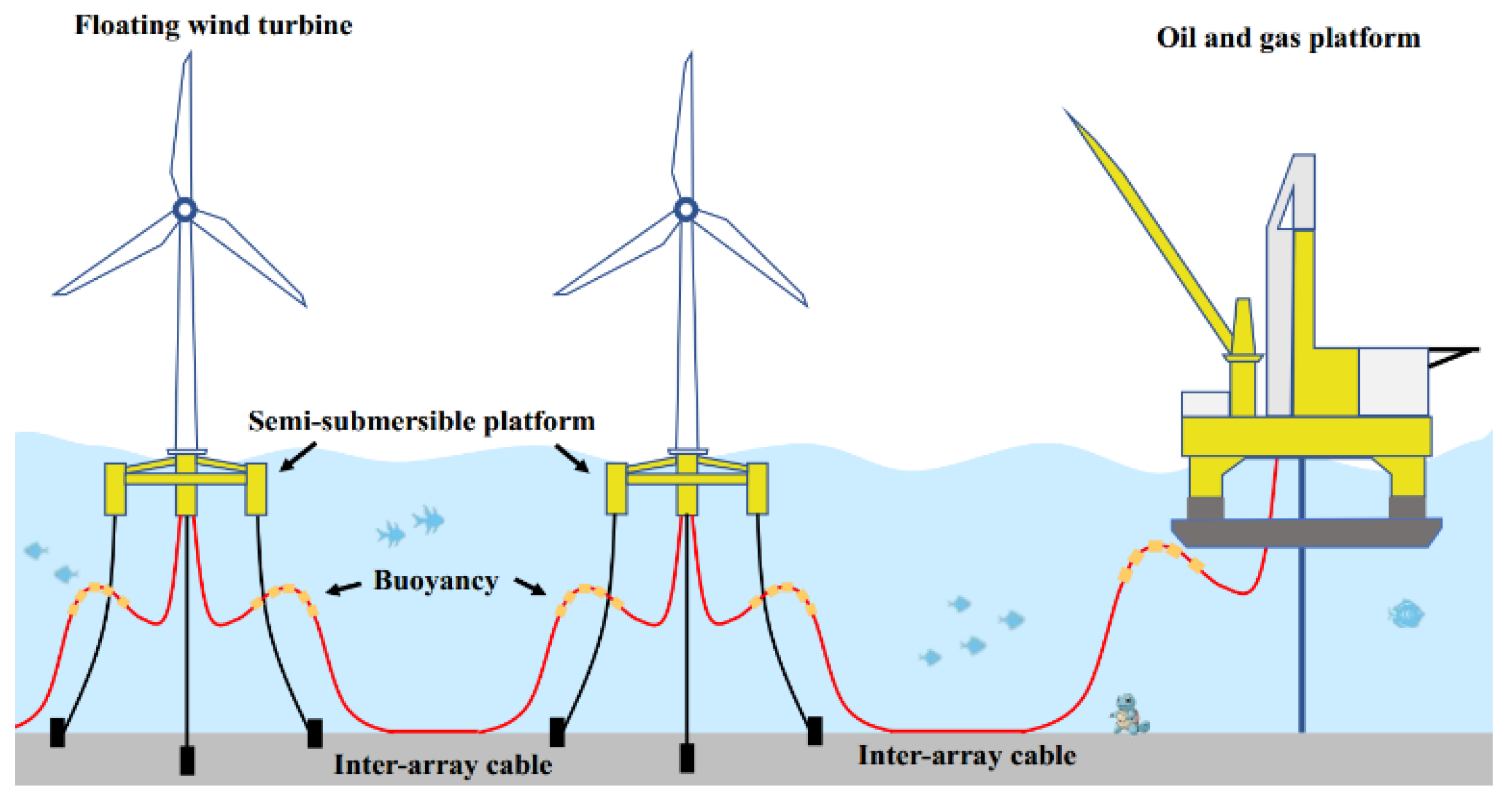
The electrical system of an FOWF comprises various dynamic submarine cables connecting FOWTs and transmitting energy to OOGPs, which can be regarded as an alternative offshore substation (Figure 1).
These cables generally consist of three-core copper conductors, reinforced with steel wire armoring and insulated components, and are designed to operate at a nominal voltage of 33 kV. Nevertheless, the advancement of more powerful FOWTs demands higher voltage levels, such as 66 kV, to reduce power loss [41]. Unlike cables for bottom-fixed wind farms buried beneath the seabed, FOWTs cables include a dynamic segment that moves with the floating substructure [42].
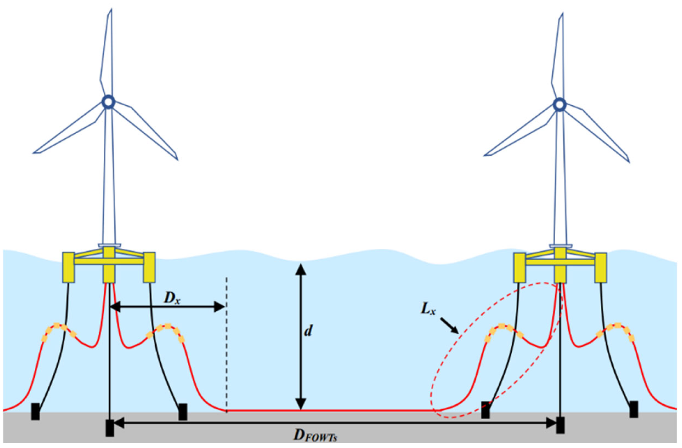
The dynamic cable in an FOWF requires robust mechanical strength and flexibility to endure the combined effects of waves, currents, seabed interactions, and the movements of the floating substructure [41]. One feasible configuration is the lazy wave, which is commonly used in offshore oil and gas risers [43]. This study adopts the lazy wave shape (Figure 2) for dynamic cables, as seen in projects like Hywind Scotland and Fukushima [44,45].
However, optimizing the electrical layout of FOWTs becomes more critical due to the increased length from the dynamic cable segment, the spatial needs of the anchoring system, and the offset of the floating platform. The power cable length between two FOWTs is determined by the equation [1].
L c a b l e = 1.05 D F O W F s + 2 ( L x D x )
where the distance between FOWTs is denoted by D F O W F s , L x is the length of dynamic cable segment, and h is the hang-off height above the seabed, calculated as h = d 20 m, where d is the water depth. The variable D x denotes the horizontal distance between the substructure and touchdown location on the seabed, set at 2h. The ratio of the L x to the h is typically 2.8 for favorable lazy-wave configurations [46]. Equation (1) facilitates the computation of the overall dynamic cable length between any two FOWTs given their respective positions. Utilizing FOWTs’ coordinates or positions, their distance is determined, enabling the calculation of the total cable length required for connecting the two turbines. This information is valuable for calculating the L i , j , the dynamic submarine cable length between any node i and node j in Section 2.3.

2.2. Cable Type Selection

Considering multiple cable types (referred to as Set T) available for the transfer of electrical power, it is possible to precompute and determine the most suitable cable type (denoted as t * ) for supporting a specified number of downstream OWTs k [23,28]. Determining the optimal cable type t * is based on the understanding that, for a given connection between node i and node j with a length denoted as L i j , and considering k downstream OWTs, the ideal cable type for this specific connection remains unaffected by other connections within the system. The optimal cable type t * could be determined by minimizing the cost per unit length, which encompasses both the cost associated with power losses per unit length and the investment cost per unit length:
min   t T 3 s S h s R t ( k I s ) 2 e p r i c e + C t
where h s is the duration time under wind scenario s, I s is the current generated by an individual OWT under wind scenario s (here we assume the wake effect is too small to change the optimal result), parameter e p r i c e = 0.68 refers to [16], while the unit cable resistance R t and unit cable cost C t of cable type t are defined according to Table 1.
The precomputation of cable types uses a simplified power-flow assumption only to narrow the feasible solution space and reduce computational complexity, and it does not determine the final cable type selection. The final cable layout optimization and power loss calculation fully incorporate wake-affected turbine power outputs, and the preselected cable type set is verified to cover all feasible options for large wind farms with significant wake effects. The preselection process does not affect the global optimality of the final optimization result, as the full wake effect is considered in the core MIQP model.

2.3. Problem Formulation Considering Wake Effect

In the context of CCLOP, all electrical power generated by FOWFs is directly transmitted to independent electrical grids at OOGPs, bypassing the need for onshore substations. However, managing multiple OOGPs receiving wind power introduces complexity, akin to several spanning tree models. To simplify calculations, we introduced the concept of a “virtual root,” consolidating all OOGPs into a single spanning tree model.
The wake effect is an important consideration for wind farms, as the energy output of downstream OWTs may experience a notable decrease due to the reduction in wind speed caused by upwind turbines. To estimate the power generation of OWTs while accounting for the wake effect under various wind scenarios, the Jensen wake model integrated in the method proposed in [47] is utilized in this study, which is widely adopted in offshore wind farm engineering due to its high computational efficiency and satisfactory accuracy.
The wake effect is modeled using the Jensen model [47,48]. For a downstream turbine j located at distance x i j from an upstream turbine i , the effective wind speed is:
v j = v i [ 1 1 1 C T ( v i ) ( 1 + 2 k w a k e x i j D r ) 2 ]
where v i is the free-stream wind speed at the upstream turbine i ; C T ( v i ) is the thrust coefficient, which is a function of wind speed; for the Siemens Gamesa SG 8.0-167 DD turbine used in this study, C T values are obtained from the manufacturer’s technical documentation; D r is the rotor diameter; k w a k e is the wake decay constant, which characterizes the wake expansion rate. For offshore open-sea conditions, k w a k e = 0.07 is adopted, following established practice in offshore wind engineering [47].
When multiple upstream turbines affect the same downstream turbine, the combined wind speed is computed using the kinetic energy deficit superposition method (sum of squares):
v j = v i [ 1 i u p s t r e a m ( j ) ( 1 v j i v ) 2 ]
where v j i is the wind speed at turbine j considering only turbine i as the upstream turbine, and v is the free-stream wind speed.
A sensitivity test has verified that small variations in the wake decay constant (±0.02) exert negligible effects on the optimization results. Since the theoretical improvement of the wake model itself is not the research scope in this paper, here we directly calculate P w j , s , the generated power of wind turbine j in wind scenario s based on the wake effect model [47,49,50] and the recorded wind data.
The objective function of the model minimizes the combined cost of cable investment and power losses over the electrical network’s operational lifespan. This function applies to both FOWFs and bottom-fixed offshore wind farms [1]. The CCLOP formulation is as follows:
min ψ i , j , Q i , j , k , P i , j , k , s   i = 1 N j = 1 N k = 1 K L i , j Q i , j , k [ C k + C o p e , k 1 ( 1 + r ) Y r + γ Y C r e p , k + γ ω P l o s s , f a i l h t o t a l 1000 ] + i = 1 N s = 1 S ( j = 1 N k = 1 K 3 ( P i , j , k , s I r a t e d ) 2 L i , j R k ) h s e p r i c e
ψ i , i = 0 ,   i [ 1 , N ]
i = 1 N ψ i , N = 0 ,
ψ N , j = 0 ,   j [ N s + 1 ,   N 1 ]
ψ N , j = 1 ,   j [ 1 ,   N s ]
i = 1 N ψ i , j = 1 ,   j [ N s + 1 ,   N 1 ]
j = 1 N ψ i , j N t i n ,   i [ N s + 1 ,   N 1 ]
j = 1 N ψ i , j N f d ,   i [ 1 ,   N s ]
i = 1 N j = 1 N ψ i , j = N 1
k = 1 K Q i , j , k = ψ i , j ,   i [ 1 , N ] , j [ 1 , N ]
i = 1 N k = 1 K P i , j , k , s j = 1 N k = 1 K P i , j , k , s = P w j , s ,   i , j [ 1 , N ] , s [ 1 , S ]  
0 P i , j , k , s k Q i , j , k ,   i [ 1 , N ] , j [ 1 , N ] , k [ 1 , K ] , s [ 1 , S ]
k = 1 K Q i , j , k P i n i , j , k = k = 1 K P i , j , k , 1 ,   i [ 1 , N ] , j [ N s + 1 , N ]
In the objective function in (3), the initial term signifies the cable investment cost, whereas the second term quantifies power losses cost throughout the entire lifespan of the FOWF, C o p e , k 1 ( 1 + r ) Y r denotes the present value of the total O&M cost over the wind farm lifetime, calculated by the annuity present value formula; γ Y C r e p , k is the expected total replacement cost considering the annual failure probability and design lifetime; γ ω P l o s s , f a i l h t o t a l 1000 stands for the annual expected reliability penalty cost due to power shortage caused by cable failure. The cable connection layout adheres to a spanning tree structure with N nodes and N − 1 connections, where the virtual root is represented as node N. OOGPs connected to the virtual root are denoted by numbers 1 to Ns, and FOWFs connecting to OOGPs are numbered Ns + 1 to N − 1. Equation (4) represents connection constraints, preventing nodes from connecting to themselves. Equation (5) denotes that the virtual root cannot supply power to other nodes. Equations (6) and (7) specify the connection constraints for FOWTs, stating that they cannot directly connect to the virtual root, while all OOGPs should supply power to it. Equations (8) and (9) set constraints for FOWTs, allowing each to send power to one node and receive power from at most N t i n nodes. Equation (10) represents the OOGPs constraints, limiting power reception from at most N f d nodes. Equation (11) imposes the spanning tree constraint, ensuring that the N nodes have exactly N − 1 connections. Equation (12) mandates that each built cable should support a certain number of downstream wind turbines. Equation (13) represents power flow conservation constraints. In each wind scenario s, power output from each node equals power entering the node plus the node’s power production. Note that these constraints exclude the virtual root, assuming zero power production for it and OOGPs. Equations (14) and (15) involve integer variables Q i , j , k and continuous variables P i , j , k , s . Equation (14) indicates the power existence constraints, stating that if there is a cable between nodes, there must be a power flow in each wind scenario s. Equation (15) expresses the relationship between the cables and power flow, stating that a cable supporting k downstream wind turbines will transfer k units of power flow during the wind scenario when FOWTs have full load generation.
The proposed model is suitable for deep-water scenarios in which FOWFs supply power directly to nearby OOGPs, without offshore substations or long-distance export cables to the onshore grid. The turbine positions are predetermined in the planning stage, and the optimal cable type is preselected according to the number of downstream WTs. The model may not be directly applicable to wind farms with offshore substations, co-optimization of turbine positions, or power transmission to the onshore power grid.

3. Solution Method

In this section, Benders’ decomposition is applied to address the MIQP problem. To enhance the convergence speed of the Benders’ decomposition process, we introduce two novel valid inequalities that are specifically developed in Section 3.2.

3.1. Basic Solution Process

In Section 2.3, the CCLOP is formulated as a mixed-integer quadratic programming (MIQP) problem, known for its computational intensity. The Benders’ decomposition algorithm is commonly employed for addressing mixed-integer programming problems, particularly when the remaining slave problem, post-determining the values of integer variables in the master problem, is convex [48]. To address the slow convergence, various acceleration methods like valid inequalities [51], approximation techniques [52,53,54] have been explored. Among these methods, leveraging valid inequalities derived from a detailed analysis of the problem [55] has proven effective in enhancing the convergence of Benders’ decomposition.
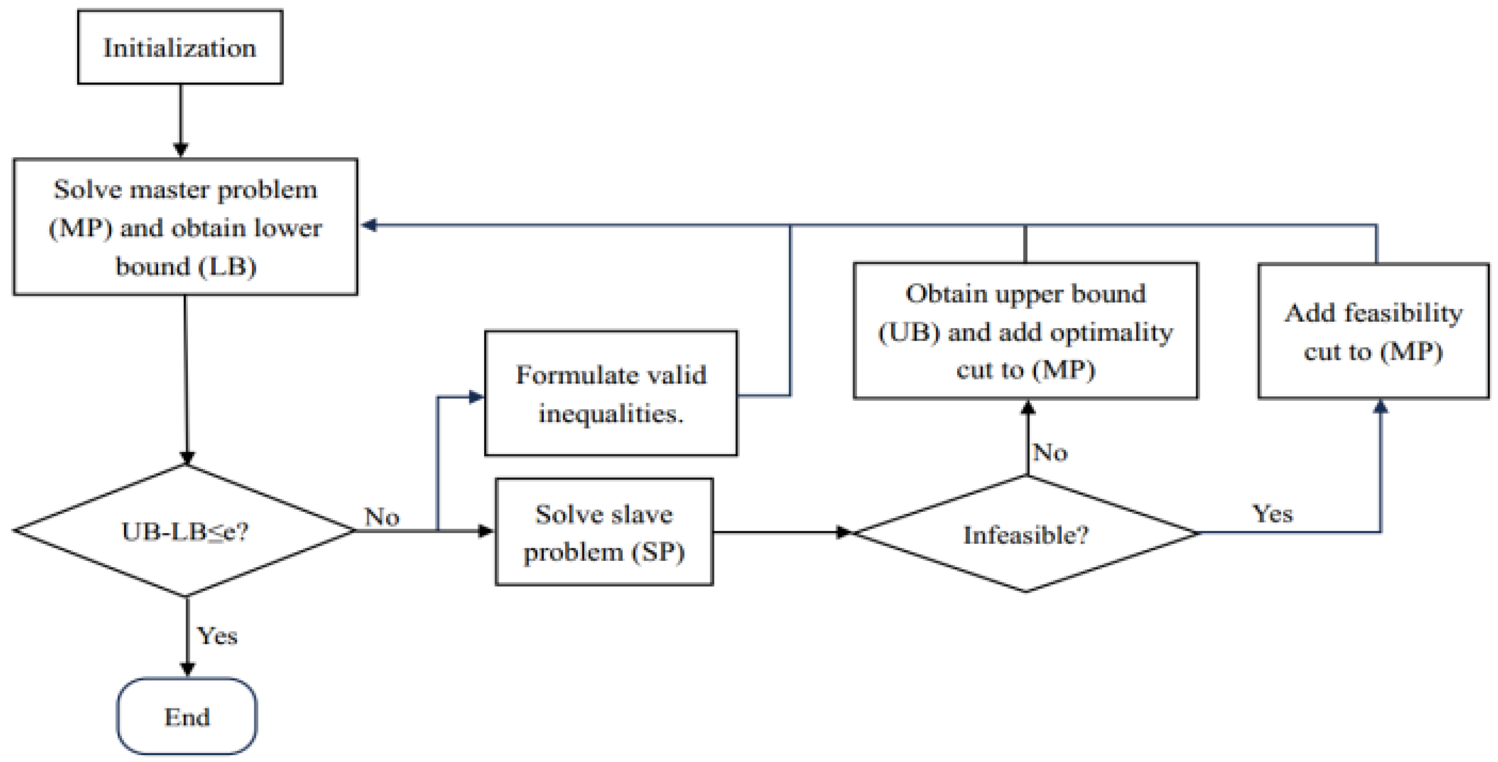
Benders’ decomposition entails partitioning the problem into a master and slave problem. The process, as illustrated in Figure 3, starts by solving the slave problem separately. Two types of cuts, either Feasibility or Optimality, will be incorporated into the master problem based on the feasibility of the outcomes. The master problem is then addressed to determine the integer variables for the next iteration and obtain a lower bound. The termination criterion is dictated by the difference between the upper and lower bounds. The primal MIQP problem can be represented as:
min x ( R + ) p , y { 0,1 } q x T H x + f T y
A x + B y b
y Y R q
In the primal problem (P), the continuous variables P i , j , k , s are non-negative, thus the vector x = v e c ( P i , j , k , s ) comprises non-negative values, and p represents the size of the vector x. Additionally, the vector y = v e c ( [ Q i , j , k , ψ i , j ] ) comprises binary variables, and q is the size of the vector y. Equation (17) represents the equivalent expression of Equations (13)–(15), which combines integer variables in y and continuous variables in x. Then, Equation (18) defines the feasible set of integer variables in y, which is equivalent to the expressions given in Equations (4)–(12). When y is fixed, the slave problem (SP) can be formulated as follows:
min x ( R + ) p x T H x + f T y ¯
A x b B y ¯
The fixed value of y, denoted as y ¯ , is established either at the start or from the outcome of the master problem in the prior step. The SP is a quadratic programming problem with a convex objective function (19), as the positive semidefinite matrix H suggests. To solve SP, methods such as interior-point convex algorithms can be employed. These methods facilitate feasibility assessment and yield the Lagrangian multipliers, denoted as λ m . Here, m represents the present count of derived optimality cuts. On the other hand, an extreme ray μ n is obtained if SP is infeasible [56], with n representing the present count of derived feasibility cuts. Next, the master problem (MP) can be formulated as follows:
min y { 0,1 } q f T y + α
0 α
λ i T ( b B y ) α , i [ 1 , m ]
μ j T ( b B y ) 0 , j [ 1 , n ]
y Y R q
(VI-1) and (VI-2)
where α is an intermediate continuous variable. Equation (21) represents the objective function of the MP. Equation (22) is utilized in the initial iteration to enforce the constraint that α remains bounded and non-negative throughout the optimization process. This constraint is crucial for maintaining the feasibility of the problem and ensuring meaningful solutions. Equation (23) denotes the optimality cuts obtained from the SP, while Equation (24) represents the feasibility cuts obtained from the SP. The proposed valid inequalities (VI-1) and (VI-2) are linear constraints elaborated in Section 3.2. The MP is a mixed-integer programming problem that can be solved via the branch-and-bound algorithm.

3.2. Development of Valid Inequalities

The core intuition of the two valid inequalities is to construct high-quality initial spanning tree structures and heuristic hybrid layouts, so as to generate effective optimality cuts and accelerate the convergence of Benders’ decomposition.
(1) VI-1: Based on the optimization results y obtained from the master problem (MP), we define the node set S i as the set of all nodes that are connected to the virtual root r through the OOGP i, where i belongs to the range [1, Ns]. In other words, S i encompasses predecessors of node i in the anti-arborescence structure, reflecting the configuration represented by y . At each iteration, the node set S i associated with OOGP i may vary. In such cases, we can perform a reoptimization of the cable connection layout using a greedy-based process:
Step 1: After obtaining the optimization results y from the MP, we can store the node set S i associated with each OOGP i. Remove node i from S i and define it as Set 1, define Set 2 as an empty set ( ), and then add node i to it. Then, Step 2 to Step 4 will be iteratively performed for i values ranging from 1 to Ns.
Step 2: Define D i as a set of distances between pairs of nodes. Specifically, it includes distances for which one node belongs to Set 1 and the other to Set 2. Then arrange these distances in increasing order. Choosing the first element d D i , which is the smallest distance, connects a node from Set 1 (denoted as node α ) to a node from Set 2 (denoted as node β ).
Step 3: If neither node α nor node β receives power from more than N t i n / N f d nodes, remove the node α from Set 1 to Set 2. Otherwise, delete the first element d D i and go back to Step 2.
Step 4: Continue with Step 2 and Step 3 until Set 1 becomes an empty set ( ).
Step 5: Obtain the integer variables y ~ based on the constructed spanning tree structure, then compare the total cost associated with y ~ to the total cost associated with y . If the cost of y ~ is lower, we substitute y ~ into the SP and solve it to obtain the corresponding Lagrangian multiplier λ m ~ . As y ~ is constructed based on the spanning tree structure, SP is always a feasible problem. Consequently, (VI-1) can be reformulated as an optimality cut:
( VI - 1 ) :   λ m ~ T ( b B y ) α
(2) VI-2: The second valid inequality arises from the hybridization of different cable connection layouts obtained from various iterations, while maintaining the same node set S i associated with OOGP i. In other words, it takes into account the combination of cable connections from different iterations that share the common set of nodes S i . This allows for the exploration of alternative cable connection configurations that leverage the best aspects of different layouts while still adhering to the constraints imposed by the fixed node set S i . The applicability of the second valid inequality depends on the availability of different cable connection layouts for the current node set S i . This means that if there are no alternative cable connection layouts for the same node set S i from previous iterations, the second valid inequality may not be applicable. The cable connection layout is reoptimized by a heuristic method:
Step 1: Obtain the cable connection layout associated with S i from the current MP optimization results y . Then, there are three scenarios to be discussed. In the first scenario, if the cable connection layout for S i is different from previous iterations but shares the same set of nodes, we add it to the layout set and define them as Set L i t . Here, i represents the node set associated with OOGP i, and t denotes the t t h version of predecessors that connect with node i. In the second scenario, if both the cable connection layout and the set of nodes are different from previous iterations, we add the new layout to the Set L i t + 1 . In the final scenario, if both the cable connection layout and the set of nodes have already been covered in previous iterations, there is no need to consider the heuristic process for this particular scenario.
Step 2: If there are multiple OOGPs whose node sets, S i , meet the first scenario (where the layout is different, but the set of nodes is the same compared to previous iterations), a random selection is made among them to perform the hybridization process.
Step 3: Randomly select one of the layouts from Set L i t and replace the current layout in S i . The selection process favors layouts with lower total costs, assigning them a higher probability of being chosen. Here, we denote the layout cost of Set L i t as Set C i t , create an intermediate set Z i t = C i t / m a x ( C i t ) , and then apply the softmax function to obtain the probability set P i t = s o f t m a x ( Z i t ) , ensuring that layouts with lower costs have higher probabilities.
Step 4: If an improved solution is found after replacing the cable connection layout in Step 3, proceed to select a new OOGP in Step 2 and repeat Step 3. However, if an improved solution is not found, continue randomly selecting new layouts from Set L i t until either an improved outcome is achieved or the specified iteration limit is reached, then proceed to select a new OOGP in Step 2 and repeat Step 3.
Step 5: Once the heuristic process has traversed all OOGPs that meet the first scenario, the reoptimized integer variables y ¨ are obtained based on the constructed spanning tree structure. The total cost associated with y ¨ is then compared to the total cost associated with y . If the cost of y ¨ is lower, y ¨ is used in the SP, and the problem is calculated to find the corresponding Lagrangian multiplier λ m ¨ . Since y ¨ is constructed based on the spanning tree structure, the SP is always a feasible problem. Therefore, (VI-2) can also be reformulated as an optimality cut:
( VI - 2 ) :     λ m ¨ T ( b B y ) α
Both valid inequalities are generated from feasible spanning tree structures that satisfy all constraints of the original problem. Since they only add optimality cuts (not feasibility cuts), they cannot exclude the true optimal solution but only tighten the feasible region of the master problem.


4. Case Study

In this part, we conduct a comprehensive assessment of the devised approach for the MIQP model. To ensure a comprehensive evaluation, we consider 32 different cases, factoring variables like the number of FOWTs, OOGPs, different placements (specifically, the distance between FOWTs in the dominant wind direction), and diverse wind data sets. Specific conditions for each case are provided in Table 2. However, determining the optimal placement of wind turbines [57,58,59] falls outside the purview of this paper. Therefore, we assume predetermined wind turbine positions. Given the current limited number of FOWFs integrated with OOGPs worldwide [17], tested cases adhere to technical standards and industrial experience [47]. This ensures that our evaluation reflects real-world conditions and best practices in the industry.
We take inspiration from the Hywind Tampen Floating Offshore Wind Farm [17] and use the Siemens Gamesa SG 8.0-167 DD 8 MW offshore wind turbine in the tested cases. This FOWT model features cut-in, cut-out, and rated wind speeds of 3 m/s, 25 m/s, and 12 m/s. The nominal operating voltage of the dynamic submarine cable system is set at 66 kV. The wind farm is located in a hypothetical sea area with a water depth of 300 m, with an expected 25-year lifespan. All generated energy is assumed to be used by OOGPs, priced at 0.15 €/kWh for the first decade, followed by a market price of 0.05 €/kWh with an interest rate of 5%.
For model validation, three 66 kV inner-array cables are used, each with specifications listed in Table 3. Furthermore, based on precomputation conducted in Section 2.2, we can see that Type 1 cable is the optimal choice for supporting 1–3 downstream wind turbines, Type 2 cable is ideal for 3–5 turbines, and Type 3 cable is suitable for 6–7 turbines.
This section includes two comparative studies. The first study compares the proposed method, which combines Benders’ decomposition with Valid Inequalities (BD + VIs), with other existing methods. The objective is to evaluate the performance and efficacy of the devised approach in relation to alternative approaches. The second study compares optimized results considering wind scenarios with wake effect and those neglecting the wake effect, providing insights into the wake effect’s impact on the optimization results.

4.1. Methods Comparison

The performance evaluation of the devised Benders’ decomposition method, BD + VIs, in the context of CCLOP involves a comparison with two other conventional optimization methods for MIQP problems. The first approach employed relies on Gurobi Optimizer, a commercial optimization solver, utilizing the branch and bound method. The second method is a custom Benders’ decomposition (BD) method [51]. The evaluation is conducted using Gurobi version 9.1.2 with default options, executed through the YALMIP toolbox in MATLAB R2022b. On the other hand, the BD method and the devised BD + VIs method are executed using custom MATLAB scripts.
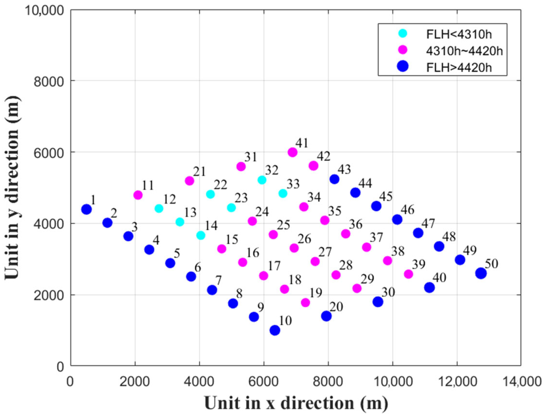
The experiment begins by inputting geographic data for OOGPs and FOWTs into the system, calculating dynamic cable lengths between each pair of nodes, employing the method outlined in Section 2.1. Subsequently, onsite wind data generates a set of 48 wind scenarios, as shown in Table 4. The wake-effect model calculates the power output for each FOWT in each scenario, as illustrated in Figure 4 (Case 32, which includes 50 FOWTs, 8 OOGPs, a distance of 10 rotor diameters (RD) in the prevailing wind direction, and wind data set 1). Different colors represent the range of annual average full-load hours (FLH) for each individual FOWT, highlighting the predominant wind direction from the southwest to southeast. Finally, the prepared data, including the geographic information, wind scenarios, and power output calculations, is fed into the optimization solvers to minimize the objective function and obtain the optimal cable configuration. By following this experimental procedure, the proposed method’s performance and effectiveness in solving the MIQP model can be thoroughly evaluated.
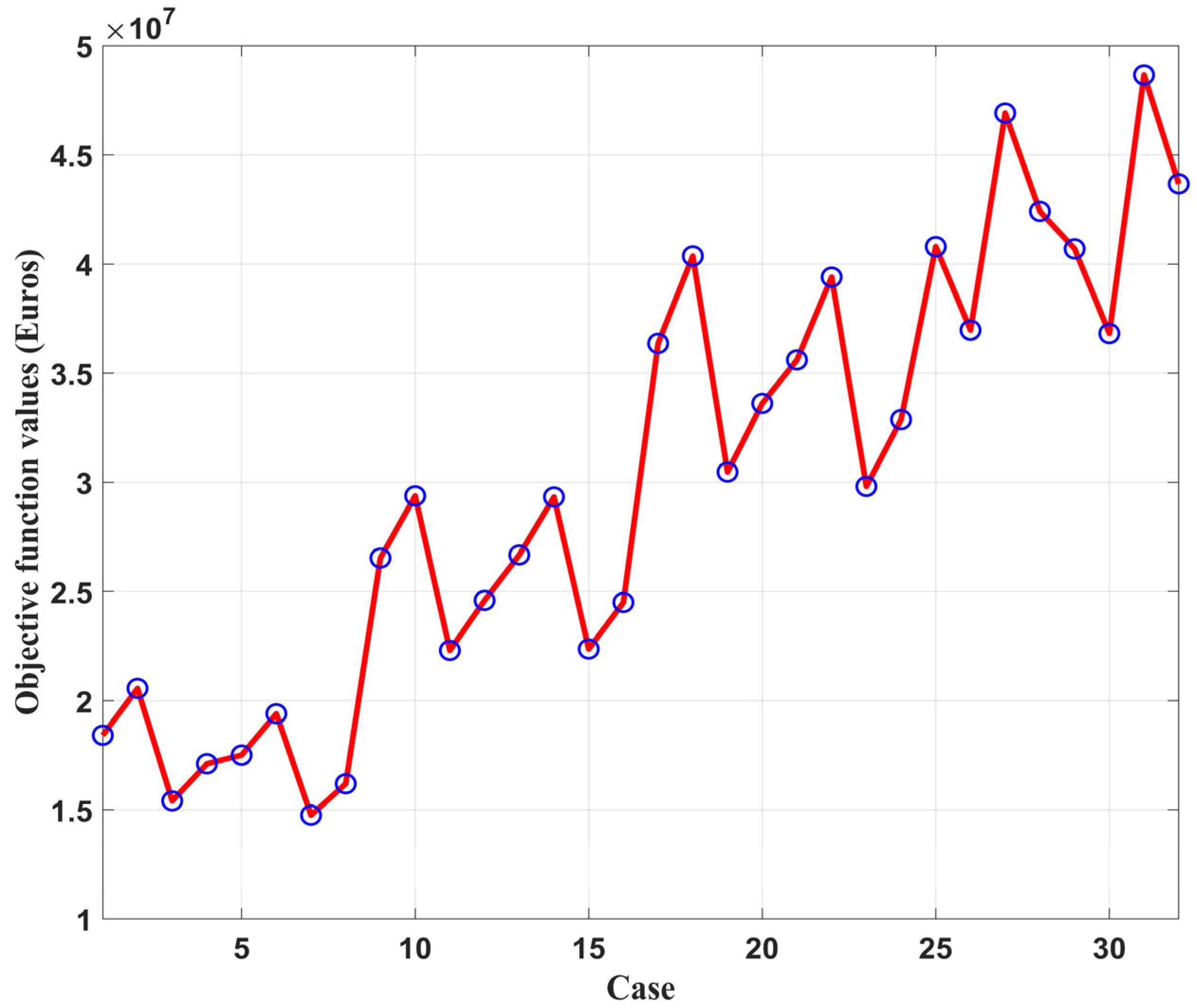
In Figure 5, the objective function values of the 32 cases of the CCLOP are displayed, providing an overview of the optimization outcomes. To compare the computational performance of the methods (Gurobi, BD, and BD + VIs).
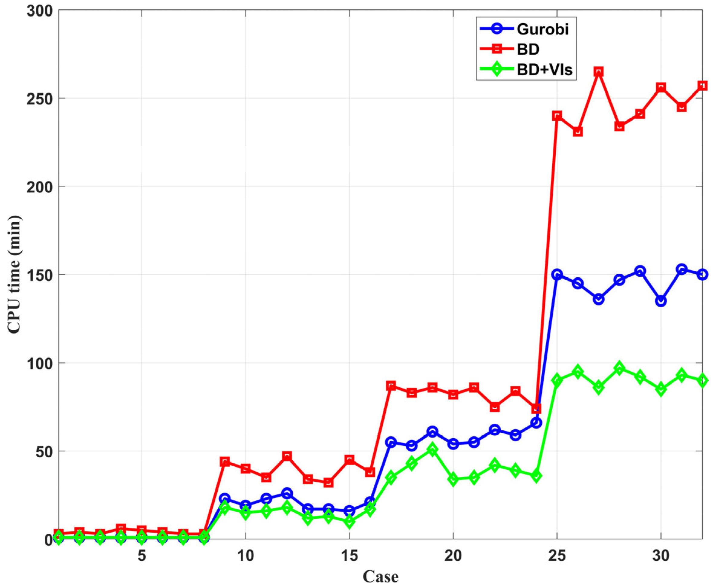
Figure 6 shows the CPU times required to solve the 32 cases. On average, the Gurobi solver takes 56.3 min, the BD method takes 92.9 min, and the BD + VIs method takes 36.6 min. It is worth noting that all methods are capable of converging to the global optimal results. The results indicate that the BD method has a slower solving speed compared to the commercial solver Gurobi. Nonetheless, among the methods investigated in this article, the BD + VIs method showcases the swiftest solving speed. In particular, BD + VIs slashes computation times by approximately 53.8% compared to the Gurobi solver. Additionally, the computational time of BD + VIs is, on average, 39.4% of that of BD alone. These findings highlight the efficacy of the devised Valid Inequalities (VIs) in reducing computation time, particularly when compared to BD without incorporating the proposed valid inequalities.

4.2. The Influence of Wake Effect on the Optimization Results

This section analyzes the influence of wake effect and power-loss calculation methods on optimization results. Four optimization models with gradually more realistic assumptions are established as a sensitivity study, so as to show how the optimal cable layout varies with the fidelity of wind power modeling.
Model 1: (Cable CapEx): Only cable investment cost (Cable CapEx) is considered, while power loss cost (PLC) is ignored.
Model 2: (Cable CapEx + PLC-FLH): Both cable investment cost and power loss cost are included, where power loss is calculated based on annual average full-load hours (FLH).
Model 3: (Cable CapEx + PLC-DWS): Power loss cost is calculated under multiple different wind scenarios (DWS), but the wake effect is not considered.
Model 4: (Cable CapEx + PLC-WE): Power loss cost is calculated under multiple wind scenarios with full consideration of the wake effect (WE), representing the most realistic condition.
To clarify the components of each model, a summary is provided in Table 5a.
Comparing Model 4 to the other three models, as presented in Table 5, underscores the significance of accounting for power losses. This inclusion results in a notable reduction in total costs, ranging from 3.64% to 7.32%. For smaller-scale wind farms (20 WTs), the disparities among models are relatively negligible, with the difference even at 0.003% between Model 3 and Model 4. This suggests that factoring in the wake effect may not be imperative with a limited number of wind turbines. However, as the wind farm’s scale expands, the distinctions among models become more conspicuous. The gap between Model 2 and Model 4 increases from 0.89% to 1.71%, and that between Model 3 and Model 4 rises from 0% to 1.11%. Consequently, for larger wind farms (over 50 WTs), considering the wake effect proves advantageous, with increasingly apparent disparities favoring Model 4 over the other models.
It is important to emphasize that the cost differences reported in Table 5b (e.g., Model 3 vs. Model 4) do not represent the “error” or “suboptimality” of the simpler models when applied to a real wind farm. Rather, they quantify the sensitivity of the optimal cable layout to different modeling assumptions. In other words, if a planner used Model 2 (FLH-based) instead of Model 4 (wake-aware) to design the cable system for a 50-WT wind farm, the resulting layout would have a total cable-related cost that is, on average, 1.71% higher than the layout obtained under the more realistic assumptions of Model 4. This 1.71% difference is the cost of ignoring wake effects and wind variability in the design phase. However, for small wind farms (20 WTs), the difference is negligible (<0.1%), indicating that simpler models may be sufficient for preliminary design or when data are limited.
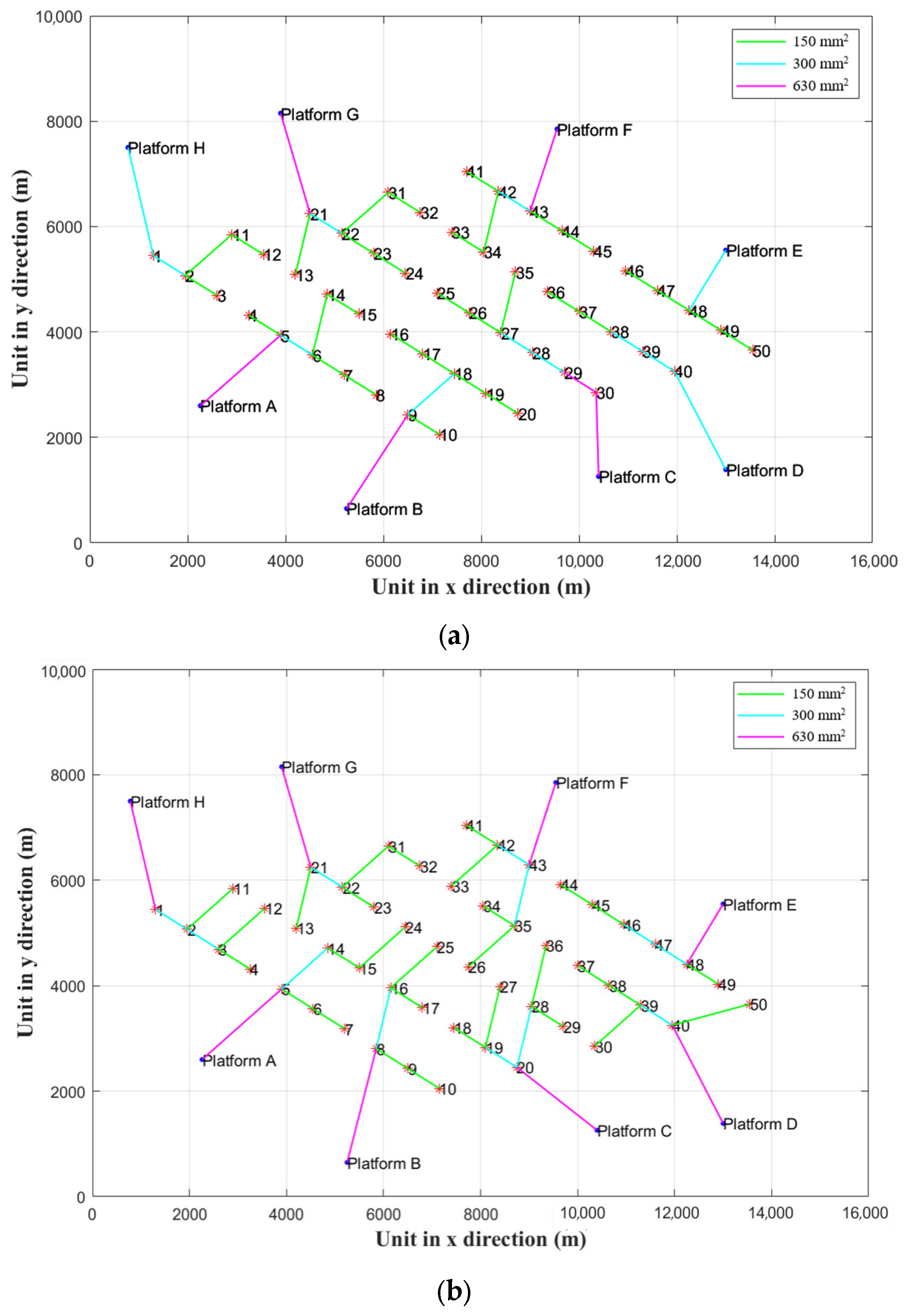
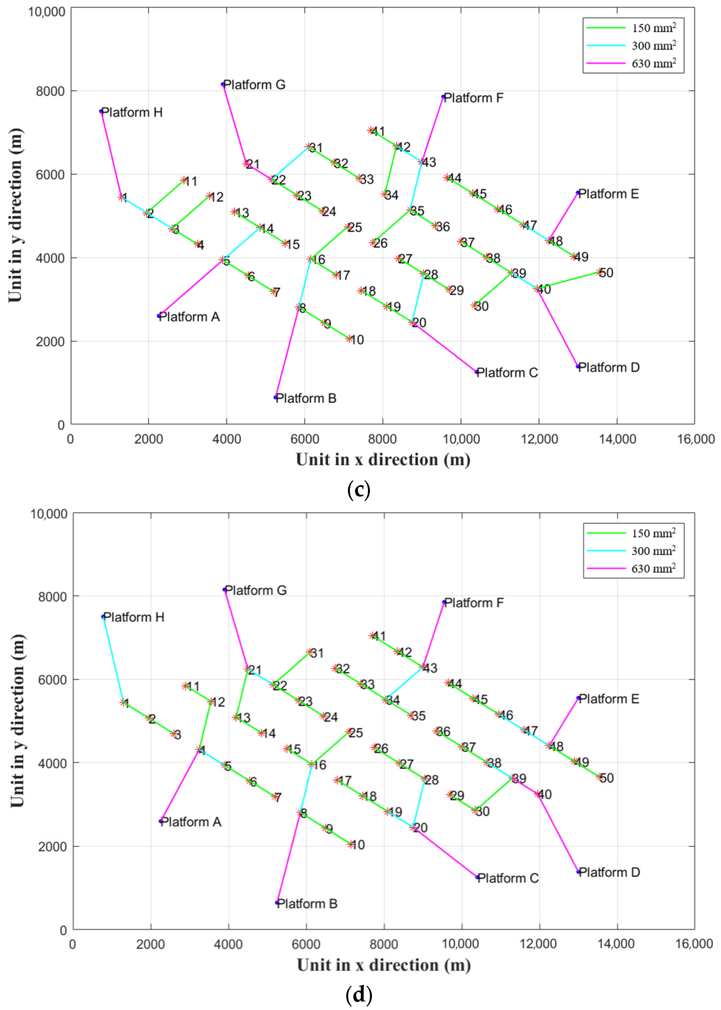
Table 5b presents a comparison of the four optimization models in Case 32. Model 1 stands out by achieving the lowest cable CapEx, beating Model 2, Model 3, and Model 4 by margins of 13.87%, 12.08%, and 3.87%, respectively. However, Model 1 sacrifices by having a significantly higher PLC, exceeding those of Model 2, Model 3, and Model 4 by 23.88%, 22.85%, and 16.22%. This is because Model 1 focuses solely on minimizing cable costs, neglecting the impact of power losses, thereby leading to the shortest total cable length. In contrast, Model 2 overestimates power losses as it assumes all wind turbines run at full capacity for a certain time, leading to inflated cable costs.
Table 6 presents a comparison of the four optimization models in Case32. Model 1 achieves the lowest cable CapEx by using shorter cables and fewer high-section cables, but this leads to higher current density and more significant power loss, resulting in a much higher PLC. By contrast, Model 2 overestimates power loss and thus tends to use more expensive large-section cables, increasing cable CapEx. Model 4 achieves a quantitative trade-off between cable investment and power loss by using an accurate wind power calculation considering the wake effect. It avoids excessive investment in large-section cables while controlling power loss within a reasonable range, which is physically consistent with the power-flow distribution and economically favorable for life-cycle cost reduction.
Remark: It is worth noting that the cable-type precomputation described in Section 2.2 is based on rated-current (full-load) assumptions and is therefore independent of wake effects. This is a deliberate design choice: cable thermal sizing must accommodate peak possible currents (e.g., during high-wind periods with no wake), whereas power-loss cost calculations require accurate modeling of actual energy production under wake-affected conditions. The two steps serve different purposes and are not inconsistent. The results in Table 5b and Figure 7 confirm that the optimization model with full wake consideration (Model 4) achieves the best trade-off between cable investment and power losses.
In practice, individual WTs frequently operate below their maximum rated power owing to the inherent variability of wind and the influence of the wake effect. Model 4 emerges as a promising choice, striking a favorable balance between PLC and cable CapEx, as depicted in Figure 7d. For instance, Model 1 (Figure 7a) selects just 5 cables with a 600 mm2 sectional area that connect to OOGPs, while Model 2 (Figure 7b) opts for 8. Model 1’s objective is to avoid costly cable types, whereas Model 2 tends to overestimate power losses, requiring larger cable areas to mitigate them. Model 4, in its quest for cost-effectiveness, chooses 7 cables, each with a 600 mm2 sectional area. Although Model 4 entails a longer computational time compared to Model 1, this is well within reason for cable layout optimization during the planning phase.
The analysis shows that, as wind farm scale increases, the wake effect leads to three key changes in the optimal cable layout:
Cable routing adjustment: Larger wind farms adopt longer cables to avoid severe wake zones, where turbines have lower and more volatile power output.
Cable type selection: Cable cross-sections are adjusted to reduce power loss in high-wake regions, with more large-section cables used for lines connecting turbines in severe wake areas.
Topological structure change: The number of cables directly connected to OOGPs increases with wind farm scale, to reduce the cumulative power loss from long transmission chains in wake-affected areas.
To assess whether the optimal cable layout is materially affected by the assumed lazy-wave parameters, we varied L x / h from 2.4 to 3.2 (±14%) and D x / h from 1.7 to 2.3 (±15%) for a representative case (Case 32: 50 WTs, 8 OOGPs, 10 RD placement). The geometric ratios were varied such that the resulting dynamic cable length changed by approximately ±10%. The full optimization (Model 4) was re-run for each variation.
Table 7 shows that the optimal cable connection topology (i.e., which turbine connects to which) and cable type selection remain nearly unchanged, with the total cost variation less than 0.5%. This verifies the robustness of the optimized layout to the dynamic segment length assumptions.

5. Conclusions

This paper has introduced a novel MIQP model to address the cable connection layout optimization problem. Firstly, a virtual root is introduced to enhance the model simplicity, connecting OOGPs and FOWTs in a spanning tree model. Subsequently, wake effect and power output variability are incorporated to accurately calculate the power losses under various wind scenarios. In addition, an accelerated Benders’ decomposition algorithm with two valid inequalities is used, which utilizes a heuristic hybridization process that incorporates various cable connection layouts and a greedy-based spanning tree structure. Our BD + VIs method exhibits an average computing time equal to 65.0% of the Gurobi solver and 39.4% of the BD method, presenting its superior computational performance in addressing the CCLOP.
Moreover, this is the first study to delve into the influence of the wake effect on the CCLOP of FOWFs across a spectrum of scales. Based on the analysis of 32 cases, the results reveal that when dealing with a limited number of WTs, the wake effect may not be obvious. However, as the wind farm scale expands, the impact of the wake effect becomes increasingly significant. Models that incorporate power losses and wake effect exhibit substantial cost reductions, ranging from 3.64% to 7.32% when compared to models that overlook these factors. Given the trend towards larger offshore wind farms in the future, it is strongly recommended to integrate the wake effect into CCLOP. It should be emphasized that the proposed model focuses on cable connection layout optimization of the power collection system rather than full-system economic evaluation, such as LCOE or overall energy yield assessment. The wake effect is reflected through cable investment and power loss cost, which is consistent with the research scope of the power collection system.
In the future, inspired by this paper, several areas warrant further improvement: (i) exploring the integration of offshore hydrogen production platforms to absorb surplus electricity and mitigate wind power volatility caused by unpredictable wind patterns; (ii) incorporating offshore wind farms with varying wind turbine capacities into the CCLOP, thus establishing a standard optimization framework.

Author Contributions

Conceptualization, T.W. and R.J.; methodology, T.W.; software, R.J.; validation, T.W., R.J. and P.H.; formal analysis, T.W.; investigation, R.J.; resources, P.H.; data curation, T.W.; writing—original draft preparation, T.W.; writing—review and editing, R.J.; visualization, T.W.; supervision, R.J.; project administration, P.H.; funding acquisition, P.H. All authors have read and agreed to the published version of the manuscript.

Funding

This work was supported by the project “Research Program on the Construction of Multi-energy Coupled Energy Systems in Typical Coastal Areas”; (Project No. 2024SSYS0071), under the “Pioneer and Leading Goose + X” Research and Development Program of Zhejiang Province and the project “Deep-Sea Offshore Wind Resource Assessment and Intelligent Planning Collaborative Platform: Development and Demonstration”; (Project No. 2026LDC01055(GZ)). Funded by the Zhejiang Provincial Major Science and Technology Project (Project No. 2026LDC01053(GZ)). The results presented in this paper are part of the outcomes of these projects.

Data Availability Statement

The original contributions presented in this study are included in the article. Further inquiries can be directed to the corresponding author.

Conflicts of Interest

Authors Tongyu Wang, Peng Hou, and Rongsen Jin were employed by the company Baima Lake Laboratory Co., Ltd. The remaining authors declare that the research was conducted in the absence of any commercial or financial relationships that could be construed as potential conflicts of interest.

References

  1. Lerch, M.; De-Prada-Gil, M.; Molins, C. A metaheuristic optimization model for the inter-array layout planning of floating offshore wind farms. Int. J. Elec. Power Energy Syst. 2021, 131, 107128. [Google Scholar] [CrossRef] [Scilit]
  2. Global Wind Energy Council. GWEC Global Wind Report 2024. Available online: https://www.gwec.net/reports/globalwindreport/2024 (accessed on 20 April 2026).
  3. Global Wind Energy Council. Global Wind Report—Annual Market Update 2017. Available online: https://marketintelligence.gwec.net/global-wind-report-2017/ (accessed on 20 April 2026).
  4. WindEurope. Floating Offshore Wind Vision Statement. 2017. Available online: https://emis.vito.be/sites/emis/files/articles/3331/2018/Floating-offshore-statement.pdf (accessed on 20 April 2026).
  5. U.S. Energy Information Administration (EIA). Offshore Production Nearly 30% of Global Crude Oil Output in 2015. 2016. Available online: https://www.eia.gov/todayinenergy/detail.php?id=28492#:~:text=Global%20offshore%20oil%20production%20(including,declines%20from%202010%20to%202013 (accessed on 20 April 2026).
  6. Global Wind Energy Council. GWEC Global Wind Report 2022. 2022. Available online: https://www.gwec.net/reports/globalwindreport/2022 (accessed on 20 April 2026).
  7. He, W.; Uhlen, K.; Hadiya, M.; Chen, Z.; Shi, G.; del Rio, E. Case Study of Integrating an Offshore Wind Farm with Offshore Oil and Gas Platforms and with an Onshore Electrical Grid. J. Renew. Energy 2013, 2013, 607165. [Google Scholar] [CrossRef] [Scilit]
  8. Haces-Fernandez, F.; Li, H.; Ramirez, D. Assessment of the potential of energy extracted from waves and wind to supply offshore oil platforms operating in the Gulf of Mexico. Energies 2018, 11, 1084. [Google Scholar] [CrossRef] [Scilit]
  9. Årdal, A.R. Feasibility Studies on Integrating Offshore Wind Power with Oil Platforms. Master’s Thesis, Department of Electric Power Engineering, Norwegian University of Science and Technology, Trondheim, Norway, 2011. [Google Scholar]
  10. Riboldi, L.; Cheng, X.; Farahmand, H.; Korpås, M.; Nord, L. Effective Concepts for Supplying Energy to a Large Offshore Oil and Gas Area under Different Future Scenarios. Chem. Eng. Trans. 2017, 61, 1597–1602. [Google Scholar]
  11. Hyttinen, M.; Lamell, J.O.; Nestli, T.F. New application of voltage source converter (VSC) HVDC to be installed on the gas platform Troll A. In Proceedings of the Cigre Session, New Delhi, India, 21–23 July 2004; p. B4-210. [Google Scholar]
  12. Korpås, M.; Warland, L.; He, W.; Tande, J.O. A case-study on offshore wind power supply to oil and gas rigs. Energy Procedia 2012, 24, 18–26. [Google Scholar] [CrossRef] [Scilit]
  13. Årdal, A.R.; Undeland, T.; Sharifabadi, K. Voltage and frequency control in offshore wind turbines connected to isolated oil platform power systems. Energy Procedia 2012, 24, 229–236. [Google Scholar] [CrossRef] [Scilit]
  14. Kolstad, M.L.; Sharifabadi, K.; Årdal, A.R.; Undeland, T.M. Grid integration of offshore wind power and multiple oil and gas platforms. In Proceedings of the 2013 MTS/IEEE OCEANS-Bergen, Bergen, Norway, 10–14 June 2013; pp. 1–7. [Google Scholar]
  15. Marvik, J.I.; Øyslebø, E.V.; Korpås, M. Electrification of offshore petroleum installations with offshore wind integration. Renew. Energy 2013, 50, 558–564. [Google Scholar] [CrossRef] [Scilit]
  16. Årdal, A.R.; D’Arco, S.; Torres-Olguin, R.E.; Undeland, T.; Sharifabadi, K. Parametric sensitivity of transients in an islanded system with an offshore wind farm connected to an oil platform. In Proceedings of the 2011 14th European Conference on Power Electronics and Applications, Birmingham, UK, 30 August–1 September 2011; pp. 1–10. [Google Scholar]
  17. NS Energy. Hywind Tampen Floating Offshore Wind Farm, 2023. Available online: https://www.nsenergybusiness.com/projects/hywind-tampen-floating-wind-farm/ (accessed on 20 April 2026).
  18. Abdallah, A.; William, M.A.; Moharram, N.A.; Zidane, I.F. Wake-resolved 3D CFD analysis of a J-blade vertical axis wind turbine: Startup optimization and tip-speed trade-offs. Eng. Sci. Technol. Int. J. 2026, 77, 102364. [Google Scholar] [CrossRef] [Scilit]
  19. Offshore Wind Biz. China’s First Deep-Sea Floating Wind Turbine Heads Offshore. 2023. Available online: https://www.offshorewind.biz/2023/03/27/chinas-deep-sea-floating-wind-platform-heads-offshore/ (accessed on 20 April 2026).
  20. McKenna, R.; D’Andrea, M.; González, M.G. Analysing long-term opportunities for offshore energy system integration in the Danish North Sea. Adv. Appl. Energy 2012, 4, 100067. [Google Scholar] [CrossRef] [Scilit]
  21. Ling-Ling, H.; Ning, C.; Hongyue, Z.; Yang, F. Optimization of large-scale offshore wind farm electrical collection systems based on improved FCM. In Proceedings of the International Conference on Sustainable Power Generation and Supply (SUPERGEN 2012), Hangzhou, China, 8–9 September 2012; pp. 1–6. [Google Scholar]
  22. Jin, R.; Hou, P.; Yang, G.; Qi, Y.; Chen, C.; Chen, Z. Cable routing optimization for offshore wind power plants via wind scenarios considering power loss cost model. Appl. Energy 2019, 254, 113719. [Google Scholar] [CrossRef] [Scilit]
  23. Fischetti, M.; Pisinger, D. Optimizing wind farm cable routing considering power losses. Eur. J. Oper. Res. 2018, 270, 917–930. [Google Scholar] [CrossRef] [Scilit]
  24. Svendsen, H.G. Planning tool for clustering and optimized grid connection of offshore wind farms. Energy Procedia 2013, 35, 297–306. [Google Scholar] [CrossRef] [Scilit]
  25. Qi, Y.; Hou, P.; Liu, G.; Jin, R.; Yang, Z.; Yang, G.; Dong, Z. Cable connection optimization for heterogeneous offshore wind farms via a voronoi diagram based adaptive particle swarm optimization with local search. Energies 2021, 14, 644. [Google Scholar] [CrossRef] [Scilit]
  26. Berzan, C.; Veeramachaneni, K.; McDermott, J.; O’Reilly, U.M. Algorithms for cable network design on large-scale wind farms. Mass. Inst. Technol. 2011, 144, 1–24. [Google Scholar]
  27. Banzo, M.; Ramos, A. Stochastic optimization model for electric power system planning of offshore wind farms. IEEE Trans. Power Syst. 2010, 26, 1338–1348. [Google Scholar] [CrossRef] [Scilit]
  28. Cerveira, A.; de Sousa, A.; Pires, E.S.; Baptista, J. Optimal cable design of wind farms: The infrastructure and losses cost minimization case. IEEE Trans. Pow. Syst. 2016, 31, 4319–4329. [Google Scholar] [CrossRef] [Scilit]
  29. Bauer, J.; Lysgaard, J. The offshore wind farm array cable layout problem: A planar open vehicle routing problem. J. Oper. Res. Soc. 2015, 66, 360–368. [Google Scholar] [CrossRef] [Scilit]
  30. Samarakoon, H.M.; Shrestha, R.M.; Fujiwara, O. A mixed integer linear programming model for transmission expansion planning with generation location selection. Int. J. Electr. Power Energy Syst. 2011, 23, 285–293. [Google Scholar] [CrossRef] [Scilit]
  31. Zhao, M.; Chen, Z.; Blaabjerg, F. Optimisation of electrical system for offshore wind farms via genetic algorithm. IET Renew. Power Gener. 2009, 3, 205–216. [Google Scholar] [CrossRef] [Scilit]
  32. Gonzalez-Longatt, F.M.; Wall, P.; Regulski, P.; Terzija, V. Optimal electric network design for a large offshore wind farm based on a modified genetic algorithm approach. IEEE Syst. J. 2011, 6, 164–172. [Google Scholar] [CrossRef] [Scilit]
  33. Zhao, M.; Chen, Z.; Blaabjerg, F. Optimization of electrical system for a large DC offshore wind farm by genetic algorithm. In Proceedings of the Nordic Workshop on Power and Industrial Electronics, Trondheim, Norway, 14–16 June 2004; Volume 37, pp. 1–8. [Google Scholar]
  34. Dutta, S.; Overbye, T.J. A clustering-based wind farm collector system cable layout design. In Proceedings of the 2011 IEEE Power and Energy Conference at Illinois, Urbana, IL, USA, 25–26 February 2011; pp. 1–6. [Google Scholar]
  35. Li, D.D.; He, C.; Fu, Y. Optimization of internal electric connection system of large offshore wind farm with hybrid genetic and immune algorithm. In Proceedings of the 2008 Third International Conference on Electric Utility Deregulation and Restructuring and Power Technologies, Nanjing, China, 6–9 April 2008; pp. 2476–2481. [Google Scholar]
  36. Hou, P.; Yang, G.; Hu, W.; Chen, C.; Soltani, M.; Chen, Z. Cable connection scheme optimization for offshore wind farm considering wake effect. In Proceedings of the 2018 IEEE Congress on Evolutionary Computation (CEC), Rio de Janeiro, Brazil, 8–13 July 2018; pp. 1–8. [Google Scholar]
  37. Hou, P.; Hu, W.; Chen, Z. Optimization for offshore wind farm cable connection layout using adaptive particle swarm optimization minimum spanning tree method. IET Renew. Power Gener. 2016, 10, 694–702. [Google Scholar] [CrossRef] [Scilit]
  38. Zhang, D.; Liu, Z.; Liang, Y.; Li, C.; Zhang, J.; Hu, G. Bilevel optimization of non-uniform offshore wind farm layout and cable routing for the refined LCOE using an enhanced PSO. Ocean. Eng. 2024, 99, 117244. [Google Scholar] [CrossRef] [Scilit]
  39. Sirkis, L.; Biglu, M.; Hall, M.; Moreno, F.; Housner, S.; Lozon, E. Floating Offshore Wind Farm Array Optimization Considering Mooring Lines, Anchors, and Array Cables. In Proceedings of the Offshore Technology Conference, Houston, TX, USA, 5–8 May 2025; Paper No. OTC-35814-MS. [Google Scholar] [CrossRef] [Scilit]
  40. Hietanen, A.I.; Snedker, T.H.; Dykes, K.; Bayati, I. A novel techno-economical layout optimization tool for floating wind farm design. Wind. Energy Sci. 2024, 9, 417–438. [Google Scholar] [CrossRef] [Scilit]
  41. Srinil, N. Cabling to connect offshore wind turbines to onshore facilities. In Offshore Wind Farms Technologies, Design and Operation; Woodhead Publishing: London, UK, 2016; pp. 419–440. [Google Scholar]
  42. Taninoki, R.; Abe, K.; Sukegawa, T.; Azuma, D.; Nishikawa, M. Dynamic cable system for floating offshore wind power generation. SEI Tech. Rev. 2017, 84, 146. [Google Scholar]
  43. Chandrasekaran, S. Dynamic Analysis and Design of Offshore Structures; Springer: New Delhi, India, 2015; Volume 761. [Google Scholar]
  44. Yttervik, R. Hywind Scotland–status and plans. In Proceedings of the EERA DeepWind Conference, Trondheim, Norway, 4–6 February 2015; pp. 1–26. [Google Scholar]
  45. Yagihashi, K.; Tateno, Y.; Sakakibara, H.; Manabe, H. Dynamic cable installation for fukushima floating offshore wind farm demonstration project. In Proceedings of the 9th International Conference on Insulated Power Cables, Versailles, France, 21–25 June 2015; pp. 1–28. [Google Scholar]
  46. Rentschler, M.U.; Adam, F.; Chainho, P. Design optimization of dynamic inter-array cable systems for floating offshore wind turbines. Renew. Sustain. Energy Rev. 2019, 111, 622–635. [Google Scholar] [CrossRef] [Scilit]
  47. Hou, P.; Hu, W.; Soltani, M.; Chen, Z. Optimized placement of wind turbines in large-scale offshore wind farm using particle swarm optimization algorithm. IEEE Trans. Sustain. Energy 2015, 6, 1272–1282. [Google Scholar] [CrossRef] [Scilit]
  48. Helseth, A.; Fodstad, M.; Mo, B. Optimal hydropower maintenance scheduling in liberalized markets. IEEE Trans. Power Syst. 2018, 33, 6989–6998. [Google Scholar] [CrossRef] [Scilit]
  49. Kumaraswamy, B.G.; Keshavan, B.K.; Ravikiran, Y.T. Analysis of seasonal wind speed and wind power density distribution in Aimangala wind form at Chitradurga Karnataka using two parameter Weibull distribution function. In Proceedings of the 2011 IEEE Power and Energy Society General Meeting, Detroit, MI, USA, 24–28 July 2011; pp. 1–4. [Google Scholar]
  50. Wang, R.; Li, W. Development of wind speed forecasting model based on the Weibull probability distribution. In Proceedings of the 2011 International Conference on Computer Distributed Control and Intelligent Environmental Monitoring, Changsha, China, 19–20 February 2011; pp. 2062–2065. [Google Scholar]
  51. Rodriguez, J.A.; Anjos, M.F.; Côté, P.; Desaulniers, G. MILP formulations for generator maintenance scheduling in hydropower systems. IEEE Trans. Power Syst. 2018, 33, 6171–6180. [Google Scholar] [CrossRef] [Scilit]
  52. Nowak, I. Relaxation and Decomposition Methods for Mixed Integer Nonlinear Programming; Springer Science & Business Media: Berlin/Heidelberg, Germany, 2005; Volume 152. [Google Scholar]
  53. Wang, Y.; Zhong, H.; Xia, Q.; Kirschen, D.S.; Kang, C. An approach for integrated generation and transmission maintenance scheduling considering N-1 contingencies. IEEE Trans. Power Syst. 2015, 31, 2225–2233. [Google Scholar] [CrossRef] [Scilit]
  54. Alizadeh, A.; Fereidunian, A.; Moghimi, M.; Lesani, H. Reliability-centered maintenance scheduling considering failure rates uncertainty: A two-stage robust model. IEEE Trans. Power Deliv. 2021, 37, 1941–1951. [Google Scholar] [CrossRef] [Scilit]
  55. Fu, J.; Nunez, A.; De Schutter, B. Accelerated optimal maintenance scheduling for generation units on a truthful platform. Energy Rep. 2022, 8, 9777–9786. [Google Scholar] [CrossRef] [Scilit]
  56. Floudas, C.A.; Aggarwal, A.; Ciric, A.R. Global optimum search for nonconvex NLP and MINLP problems. Comput. Chem. Eng. 1989, 13, 1117–1132. [Google Scholar] [CrossRef] [Scilit]
  57. Hou, P.; Zhu, J.; Ma, K.; Yang, G.; Hu, W.; Chen, Z. A review of offshore wind farm layout optimization and electrical system design methods. J. Mod. Power Syst. Clean Energy 2019, 7, 975–986. [Google Scholar] [CrossRef] [Scilit]
  58. Hou, P.; Hu, W.; Soltani, M.; Chen, C.; Chen, Z. Combined optimization for offshore wind turbine micro siting. Appl. Energy 2017, 189, 271–282. [Google Scholar] [CrossRef] [Scilit]
  59. Hou, P.; Hu, W.; Chen, C.; Soltani, M.; Chen, Z. Optimization of offshore wind farm layout in restricted zones. Energy 2016, 113, 487–496. [Google Scholar] [CrossRef] [Scilit]
Figure 1. Electrical system of an FOWF integrated with an OOGP.
Energies 19 02041 g001
Figure 2. The dynamic cable connection between two turbines.
Energies 19 02041 g002
Figure 3. Basic solving framework of Benders’ decomposition.
Energies 19 02041 g003
Figure 4. Annual average equivalent FLH for each WT in Case 32.
Energies 19 02041 g004
Figure 5. Objective function values from 32 cases.
Energies 19 02041 g005
Figure 6. Assessment of CPU times using different solvers.
Energies 19 02041 g006
Figure 7. The comparison of the four optimization models in Case32: (a) Cable CapEx, (b) Cable CapEx + PLC-FLH, (c) CapEx + PLC-DWS, (d) CapEx + PLC-WE.
Energies 19 02041 g007aEnergies 19 02041 g007b
Table 1. Decision variables and parameters in MIQP model.
Decision Variables
ψ i , j Binary variable. Node j connects to Node i if ψ i , j = 1 , otherwise ψ i , j = 0 .
Q i , j , k Binary variable. Node j connects to Node i and transfers k number of turbines’ energy if Q i , j , k = 1 , otherwise Q i , j , k = 0 .
P i , j , k , s Continuous variable. Node j connects to Node i and transfers k number of turbines’ energy in wind scenario s.
Parameters
NsThe total number of OOGPs.
NThe total number of nodes, including all OOGPs, wind turbines and a virtual root.
L i , j The dynamic cable length (km) between node i and node j, which is calculated based on (1).
C t The unit cost (k€/km) of type t cable.
C k The dynamic cable cost (k€/km) associated with transferring the energy generated by k wind turbines, which is determined based on the optimization process in (4).
h s The total hours (h) in wind scenario s.
e p r i c e The electricity price (€/MWh).
R t The unit cable resistance (Ω/km) of type t cable.
R k The unit cable resistance (Ω/km) associated with transferring the energy generated by k wind turbines, which is determined based on the optimization process in (4).
P w j , s The power output (MW) of wind turbine j in wind scenario s.
I r a t e d The rated current (kA) of a wind turbine.
P i n i , j , k The index of number of wind turbines, P i n i , j , k = k .
N t i n The maximum allowable number of input cables of FOWTs.
N f d The maximum allowable number of input cables of OOGPs.
C o p e , k The annual operation and maintenance cost per unit length of dynamic submarine cable for transmitting energy from k wind turbines.
C r e p , k The cost per unit length of dynamic submarine cable for transmitting energy from k wind turbines after failure.
γ The Annual failure probability of dynamic submarine cable.
Y The design lifetime of the floating offshore wind farm.
r The discount rate.
ω The penalty coefficient for power shortage caused by submarine cable failure.
P l o s s , f a i l The power shortage due to submarine cable failure.
h t o t a l The total annual hours.
Table 2. The different conditions of the 32 tested cases.
CaseNumber of FOWTsNumber of OOGPsPlacementWind Data Set
1–8203, 48 RD, 10 RDSet 1, Set 2
9–16305, 68 RD, 10 RDSet 1, Set 2
17–24406, 78 RD, 10 RDSet 1, Set 2
25–32508, 98 RD, 10 RDSet 1, Set 2
Table 3. 66 kV inner-array cable information [1].
TypeSection Area (mm2)Power Capacity (MW)Support WTs (No.)Resistance R (Ω/km)Static Cable Cost (k€/km)Dynamic Cable Cost (k€/km)Buoyancy Components (k€)Stiffner and Connectors (k€)
11503030.1630032363145
23004050.0842345681172
36306370.04554603126231
Table 4. Time length in 48 wind scenarios with different wind directions and wind speeds.
Time Length (Hours) per Year45°90°135°180°225°270°315°
0~3 m/s4792768391927228
3~6 m/s188267253267192265263162
6~9 m/s211324235229296453283136
9~12 m/s16917518721744946426590
12~25 m/s7220117428754039738175
≤25 m/s00000480
Table 5. (a) Components included in four optimization models. (b) The average difference of optimization results between model 4 with other three models.
(a)
ModelCable CapExPower Loss CostFull-Load HoursMultiple Wind ScenariosWake Effect
1××××
2××
3××
4×
(b)
WTs No.Model 1Model 2Model 3
20 (Case 1–8)5.23%0.89%0.003%
30 (Case 9–16)7.32%1.11%0.29%
40 (Case 17–24)3.64%1.57%0.45%
50 (Case 25–32)5.06%1.71%1.11%
Table 6. Optimized layouts comparison of case 32.
Model 1Model 2Model 3Model 4
Calculation time (min)0.160.8692.1490.02
Total cable length (km)76.40583.38181.45677.2927
Total cable cost(M€)45.42444.63244.32843.671
Total PLC (M€)17.45913.28913.46914.626
Total cable CapEx (M€)27.96431.34330.85929.045
Table 7. Sensitivity of optimal layout to lazy-wave geometric parameters (Case 32).
ParameterTested RangeTopology ChangeCable Type ChangeTotal Cost Change
L x / h 2.4–3.2NoNo<0.5%
D x / h 1.7–2.3NoNo<0.5%
Disclaimer/Publisher’s Note: The statements, opinions and data contained in all publications are solely those of the individual author(s) and contributor(s) and not of MDPI and/or the editor(s). MDPI and/or the editor(s) disclaim responsibility for any injury to people or property resulting from any ideas, methods, instructions or products referred to in the content.