Article

Integration of Grid-Scaled Power-to-Heat Technology in Korea’s Power System: Operational Advantages and Future Insights for Renewable Energy Enhancement


Department of Electronic and Electrical Engineering, Hongik University, Seoul 04066, Republic of Korea
*
Author to whom correspondence should be addressed.
Energies 2026, 19(7), 1766; https://doi.org/10.3390/en19071766
Submission received: 5 February 2026 / Revised: 24 March 2026 / Accepted: 26 March 2026 / Published: 3 April 2026

Abstract

Korea’s rising shares of variable renewable energy (VRE) and inflexible baseload increases the need for fast-responding and cost-effective flexibility. Most studies on power-to-heat (P2H) emphasize district-heating (DH) economics or load shifting, leaving the system-level impacts of its reserve provision capability unclear. We develop a mixed-integer linear programming model for reserve-constrained unit commitment (RCUC) that co-optimizes the power and DH systems. In addition, the model incorporates a P2H system capable of providing multiple reserve services. Reserve requirements are divided into static and dynamic terms, with the dynamic term represented as a piecewise-linear approximation of short-term VRE variability derived from weather-based generation profiles and evaluated at the scheduled VRE output. Using a 2030 winter week for Korea, we compare five cases: no EB; EB as load only; and EB contributing only to the secondary/regulation reserve requirement, only to the primary reserve requirement, or both. Under the KRW 1000/kWh curtailment-penalty case, EB as load reduces system operating cost compared to the baseline, and enabling reserve provision yields additional cost savings, with the largest benefit observed when primary reserve is provided. EB operation also shifts dispatch from coal and gas toward nuclear, VRE, and pumped storage, while reducing renewable curtailment. Overall, enabling P2H to contribute to reserve procurement, particularly in the primary reserve, delivers substantially greater value than representing P2H solely as a controllable load for energy shifting.

1. Introduction

In response to climate change, the Government of the Republic of Korea has declared a target of carbon neutrality by 2050. According to its long-term power supply plan, the government aims to restructure the generation mix such that, by 2038, 27% of total electricity generation will be supplied by variable renewable energy (VRE), namely wind and solar power, and 35% by nuclear power as an inflexible resource [1]. As a result, the Korean power system is characterized by a high share of both inflexible and variable generation and is operated as an isolated power system, which poses substantial challenges for system operation. In practice, due to the rapid increase in solar PV capacity, nuclear power plants have been dispatched down for system stability reasons since 2023, and curtailment of renewable generation has been implemented since 2024. These issues are expected to intensify as the share of renewable generation continues to grow.
A variety of measures are being pursued to address power system stability concerns and enhance renewable energy integration. Among these, the government plans not only to develop additional energy storage facilities, such as pumped-storage hydropower plants and battery energy storage systems (BESS), to secure operating reserves, but also to deploy sector coupling technologies [1]. Sector-coupling technologies integrate the power sector with other energy sectors to improve the overall efficiency of the energy system; in other words, they link various energy sectors around electricity to promote decarbonization and the expansion of renewable energy. Among these options, power-to-heat (P2H) is a technology that converts surplus renewable electricity, which would otherwise be curtailed, into heat via electric boilers (EBs) or heat pumps (HPs) [2]. Furthermore, by controlling the power consumption of EBs and HPs, P2H resources may have the technical capability to support ancillary services [3]. However, their actual participation depends on the market design and technical requirements of the relevant power system. In addition, P2H can substitute for existing heat supply technologies such as peak load boilers (PLBs) and combined heat and power (CHP) plants, leading not only to cost reductions in the heat supply system but also to reductions in CO2 and other pollutant emissions [4]. For these reasons, the use of surplus renewable electricity for heat production via EBs or HPs is considered to have substantial potential. Therefore, it is necessary to conduct a detailed analysis of the impacts of P2H technologies with these multiple advantages.
Prior research has primarily evaluated P2H technologies from the district-heating (DH) system perspective. Ref. [5] used a cost-minimizing mixed-integer programming (MIP) model to quantify how grid-tariff structures affect the operational flexibility of EBs, indicating the importance of tariff design. Ref. [6] applied stochastic programming to the Danish power market and estimated the economic value of HPs and EBs under uncertainty, highlighting P2H’s substantial flexibility potential. Ref. [7] showed in a short-term operational model that jointly using CHP, HP, EB, and thermal energy storage (TES) increases flexibility, lowers generation costs, and expands wind accommodation. Ref. [8] integrated Balmorel with energyPRO to assess the impact of electricity-price levels and volatility on DH flexibility, finding that investment in TES and EBs is profitable during low-price periods and enhances operational flexibility. Ref. [9], using energyPRO to compare three DH system types, reported that HP adoption enhances profitability and decarbonization. Ref. [10] forecasted heat demand using neural networks and a similar-day approach and proposed EB-/TES-based flexible supply schemes, though the quantitative evaluation of flexibility and reserve contributions remained limited. Ref. [11] developed a co-optimized heat–power economic dispatch framework that includes EBs, demonstrating reduced operating costs and wind curtailment and improved system flexibility. Refs. [12,13] further showed that scheduling strategies combining EBs and TES (and, in some cases, energy storage systems (ESS) and bypass compensation technology (BCT)) can increase renewable energy absorption and system revenues. Ref. [14] proposed a Korean heat-pump water-heater (HPWH) model and found that participation in reverse demand-response programs yields 6–17% operating-cost reductions across all cases, with potential to lower the infrastructure costs of absorbing surplus renewable generation. However, most existing research focuses on DH systems and does not evaluate, at the power system level, how operating reserve provision by P2H affects total operating cost and renewable-energy curtailment.
Several studies directly examine P2H participation in ancillary service markets. Ref. [15] showed that, in the German market, when EBs provide downward automatic FRR (aFRR-down), total system costs and CO2 emissions decline; however, the study did not evaluate primary reserve and the effects on renewable-energy curtailment. Ref. [16] used heuristic optimization of residential HP clusters to assess the technical and financial feasibility of participating in the FRR market, but did not consider primary reserve. Ref. [17] showed that an ESS–P2H hybrid can reduce investment costs compared to battery-only configurations in the German primary control reserve (PCR, i.e., FCR) market, but did not evaluate secondary reserve (aFRR). Ref. [3] conducted real-time controller–hardware-in-the-loop (RT-CHIL) experiments to demonstrate the technical prequalification and performance of electric boilers and heat pumps for participation in FCR, aFRR, and mFRR. Ref. [18] formulated adaptive robust energy and reserve co-optimization under wind uncertainty and showed reductions in total operating cost, but did not sufficiently represent upward and downward reserve product differentiation, nor curtailment effects at high renewable penetration. Ref. [19] evaluated the economics of reserve market participation across alternative asset configurations and emphasized the importance of TES capacity; however, the study did not disaggregate reserves by type. Ref. [20] proposed a profit-maximizing operating strategy for a DH system with P2H technologies participating simultaneously in the energy and balancing markets (FCR/FRR/aFRR). In the context of DH decarbonization, Ref. [4] analyzed the sensitivity of DH operating costs and revenues to electricity and reserve prices, highlighting TES and reserve market participation as hedges against electricity price volatility. As summarized in Table 1, prior studies differ substantially in the reserve products considered and in the level of product specification. Although some studies examined specific reserve products in detail, many focused on selected market segments or did not systematically disaggregate reserve services by type and direction. In addition, several studies approached the problem from a DH system perspective rather than from a national power-system scheduling perspective.
Beyond the studies summarized in Table 1, there are also studies that examine the impacts of P2H technologies from a national power-system perspective. Ref. [21] showed that, in a prospective Italian power system, DH based on CHP and HPs can reduce operating costs and emissions by up to 50%, alleviate renewable energy curtailment, and cost-effectively supply up to 15% of the upward reserve requirement; however, the study did not address primary reserves. Ref. [22] analyzed Korea’s 2050 net-zero scenario at the national (power system) scale using EnergyPLAN, finding that P2H can meet approximately 14.5% of DH demand; the study further noted limitations in absorbing surplus renewable generation and therefore recommended adjustments to the generation mix, but did not consider the provision of operating reserves.
When analyzing future power systems, increasing shares of VRE generally lead to higher reserve requirements to accommodate increased VRE output variability. In [21], the reserve requirement was determined for each hour based on the maximum available VRE output in that hour. However, if renewable curtailment occurs, this capacity-based approach can overestimate the reserve requirement and thereby increase operating costs. Moreover, Reserve requirements intended to cover renewable generation variability are often quantified using statistical measures such as forecast-error-based metrics [23]. However, applying a fixed metric irrespective of curtailment or operating level may overestimate reserve requirements.
Taken together, the existing literature can be grouped into three streams: (i) DH-oriented techno-economic and flexibility studies, (ii) studies on P2H participation in ancillary-service or balancing markets, and (iii) national power system studies of sector coupling. However, an integrated assessment remains limited that simultaneously considers: (a) a reserve constrained unit commitment framework co-optimizing the power and DH systems, (b) explicit disaggregation of reserve services by product and direction, (c) reserve requirement modeling that accounts for renewable curtailment through scheduled VRE output, and (d) a quantitative case study for the Korean power system, which is characterized by high nuclear penetration, increasing VRE share, and isolated power system operation. To the authors’ knowledge, no prior study has simultaneously combined a power–DH co-optimized RCUC framework, explicit reserve-product disaggregation, curtailment-aware dynamic reserve modeling based on scheduled VRE output, and a Korean high-nuclear, high-VRE isolated-grid case study.
To address these gaps, this paper assesses the national level operational impacts of deploying grid scale P2H resources, modeled as an EB coupled with DH assets, under high VRE penetration and increasing renewable curtailment. We formulate a mixed integer reserve constrained unit commitment (RCUC) model that co-optimizes the electric power system and the DH system. On the power side, the model represents unit commitment constraints for conventional generators (nuclear, coal, and gas), CHP units with mode dependent feasible operating regions, pumped storage hydropower (PSH) operation, and VRE scheduling with curtailment. On the heat side, it enforces DH heat balance using CHP, EB, PLB, and TES, including intertemporal TES charging and discharging dynamics.
A key feature of the proposed framework is the explicit representation of operating reserve provision by P2H. The EB is modeled not only as a controllable electric load for heat production but also as a demand-side flexibility resource that can, in the modeled scenarios, contribute to upward and downward reserve requirements by adjusting its electricity consumption. Operating reserve products are disaggregated into primary and secondary/regulation reserves, and both conventional units and the EB are constrained to provide these services within their technical operating ranges. For the EB, this representation should be interpreted as a forward-looking technical assumption rather than as a direct representation of current Korean market eligibility. The resulting framework enables a power system level assessment of how EB based reserve provision affects unit commitment decisions, system costs, and renewable curtailment.
This study also addresses a reserve requirement modeling issue that becomes critical under high VRE penetration. Reserve requirements are often computed using available VRE output, which can lead to potential overestimation during intervals with renewable curtailment. To account for curtailment, we evaluate the VRE-related dynamic reserve component with respect to scheduled VRE output and embed it endogenously in the RCUC formulation. Specifically, the reserve requirement is decomposed into a static component and a dynamic component, where the latter reflects short-term VRE variability derived from weather-based generation profiles and is incorporated into the MILP through a piecewise-linear approximation. This formulation allows scheduled VRE output, reserve requirements, and unit commitment decisions to be determined simultaneously within a unified optimization framework.
The main contributions of this paper are as follows.
  • We develop an MIP based RCUC model that co-optimizes the power and DH sectors and enables EB provision of upward and downward primary and secondary regulation reserves, thereby assessing the power system level impacts of P2H based reserve provision.
  • We model the dynamic component of the reserve requirement using output-dependent short-term VRE variability derived from weather-based generation profiles and integrate it endogenously into the RCUC framework.
  • Using Korea relevant data for a 2030 case study, we evaluate the system wide impacts of EB operation under alternative reserve participation configurations.
The remainder of this paper is organized as follows. Section 2 describes the coupled power and DH systems and the modeling of CHP, EB, PLB, and TES. Section 3 presents the proposed reserve requirement formulation based on short-term VRE variability evaluated at the scheduled VRE output. Section 4 details the RCUC formulation. Section 5 reports the case study setup and results. Section 6 concludes the paper.

2. System Description

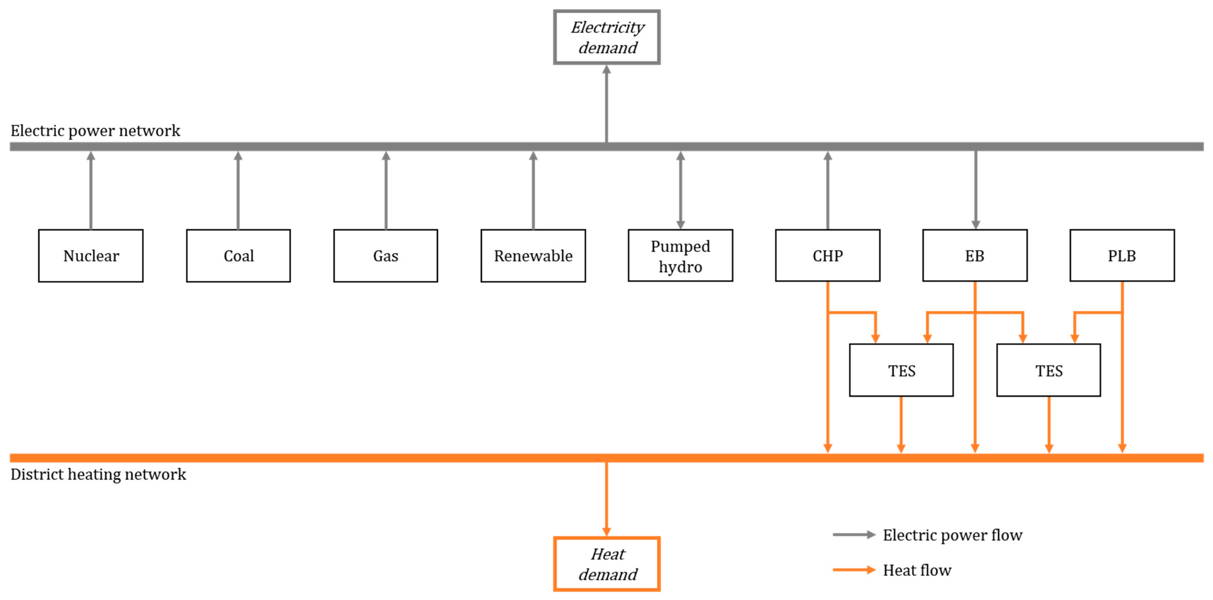
Figure 1 illustrates the system architecture incorporating P2H technologies. The overall system comprises an electric power system and a DH system. The power system meets electricity demand and includes following: thermal units (nuclear, coal-fired, and gas-fired); CHP plants; PSHs; and renewable energy sources such as wind and solar. The DH system meets heat demand and consists of CHP plants, PLBs, EBs, and TESs.

2.1. Combined and Hear Power Plant

CHP plants use fossil fuels to produce electricity and heat simultaneously, thereby supplying both the power and DH systems. The CHP plant can operate in several modes, depending on the required heat-to-electricity supply ratio. In Korea, CHP operating modes are commonly categorized into five types, summarized below [24,25].
  • Mode I (Heat-match mode): Operated primarily to supply heat, while also producing electricity. In this mode, the gas turbine (GT), heat recovery steam generator (HRSG), the high-pressure steam turbine, and the district heating network are in service. This mode generally offers the highest fuel efficiency.
  • Mode II (GT-only, emergency power mode): An emergency mode to supply electricity rapidly by operating only the GT. No heat is produced.
  • Mode III (Electricity-match mode): Operated mainly to supply electricity with no heat delivery. The GT, HRSG, high-pressure and low-pressure steam turbines, and the condenser are in service.
  • Mode IV (Emergency heat-led mode): An emergency mode to prioritize heat supply. The GT and HRSG are in service to deliver heat to DH; the GT also produces electricity.
  • Mode V (Mixed-match mode): An intermediate mode between Modes I and III that supplies both heat and electricity; the heat–power split is varied by adjusting the steam admitted to the LP steam turbine. Its efficiency is lower than in Mode I.
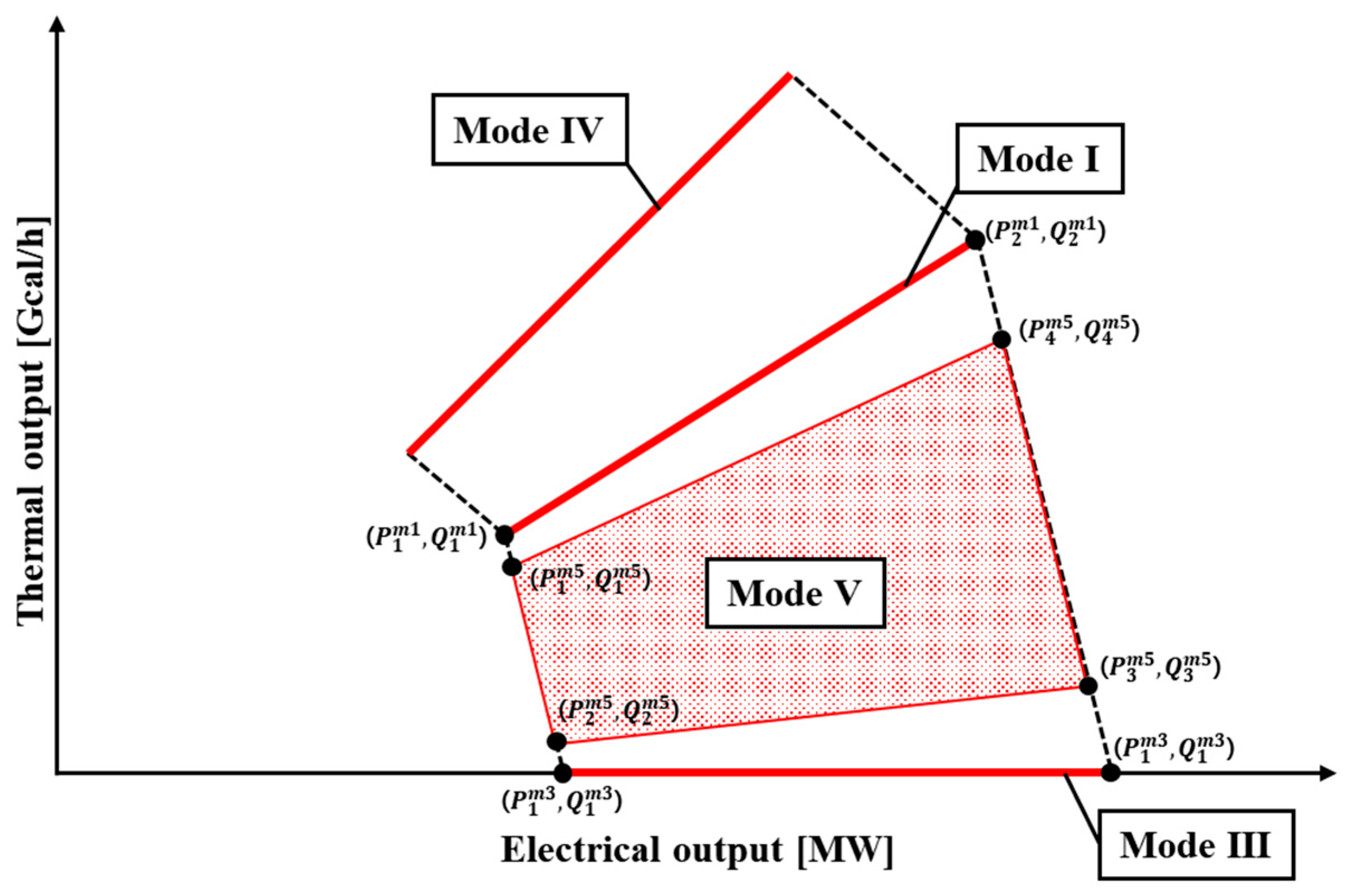
Modes II and IV are used in emergency situations. Accordingly, although CHP plants can operate in five modes in practice, the proposed RCUC model considers only Modes I, III, and V, which represent the conventional modes used in routine operation. In routine scheduling, the operating mode is selected among these three modes according to heat demand and overall energy efficiency. Figure 2 illustrates the feasible operating ranges of the modeled CHP modes (I, III, and V).

2.2. Electric Boiler and Thermal Energy Storage

Historically, when the CHP plant could not meet heat demand, heat was supplied by PLBs and/or by discharging TES. When heat demand exceeded the CHP’s heat supply capability, operators met the shortfall by starting PLBs, which have shorter start up times than CHP units, or by discharging TES. However, because PLBs produce only heat from fossil fuels, they are generally less cost-effective at the system level and entail higher emissions. By contrast, EBs convert electricity into heat. During periods of surplus electricity supply driven by VRE (or when electricity prices are low), EBs can produce heat for immediate delivery to the DH network, while any excess can be stored in TES for later use, thereby improving overall system efficiency. In this context, the TES capacity should be sized to absorb the EB’s surplus heat output over the assumed charging duration.
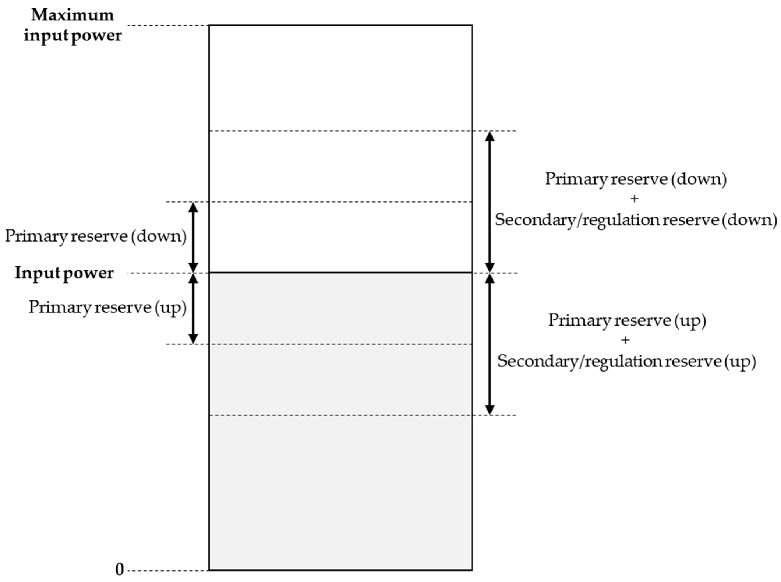
Beyond heat production, EBs can provide operating reserves to the power system as demand-side resources by adjusting their electricity consumption. Reducing consumption decreases net load and thus provides upward reserve, whereas increasing consumption provides downward reserve, as illustrated in Figure 3.

3. Reserve Requirement Considering Variable Renewable Energy

In the Korean power system, the criteria for operating-reserve requirements are as shown in Table 2 [26]. The frequency restoration reserve (FRR) is determined at a level that satisfies the system-frequency criterion in the event of the contingency (loss) of the largest generating unit (1400 MW). Under the current Korean operating rules, this definition explicitly refers to generators and ESS and does not explicitly identify transmission-connected electric loads such as industrial EBs as primary-reserve providers. Accordingly, EB participation in primary reserve is treated in this study as a forward-looking technical scenario. Secondary reserve is automatically activated through AGC to restore system frequency after the initial primary response to the loss of the largest generating unit. Tertiary reserve is manually activated to restore the reserve margin after the contingency by replacing the deployed secondary reserve. The upward regulation reserve accounts for normal load variations, whereas the downward operating reserve and downward regulation reserve account for oversupply arising from the expansion of renewable energy. Downward regulation reserve denotes reserve that can reduce generator output or increase load through automatic generation control, remote set-point control, or similar methods. Downward operating reserve is a concept that encompasses downward regulation reserve and, in addition, includes the reserve capacity of resources that, through manual actions, can reduce generator output or increase load.
The Korean power system has established reserve criteria that account for the impacts of expanding renewable generation. However, as VRE penetration increases further, revised reserve-requirement criteria will be necessary. Following [27], we adopt an n-sigma criterion to represent the additional reserve requirement associated with short-term VRE variability in each time interval. In this study, the additional reserve requirement is formulated to reflect minute-level variability derived from weather-based VRE generation profiles. Applying the method of [27] yields the reserve requirements summarized in Table 3.
Let σ v r e 1 m and σ v r e 5 m denote the standard deviations of the 1 min and 5 min VRE fluctuations, respectively, computed from weather-based VRE output data. Because these quantities are estimated for different VRE operating levels from weather-based VRE output data and may vary nonlinearly across those levels, we represent σ v r e 1 m ( p t v r e , s c h ) and σ v r e 5 m ( p t v r e , s c h ) as functions of the scheduled VRE output. Here, p t v r e , s c h denotes the scheduled VRE output determined by the unit-commitment (UC) model, subject to system constraints and bounded above by the available VRE output p t v r e , a v l .
In standard UC formulations, reserve requirements are typically treated as exogenous, precomputed parameters and are evaluated with respect to the available VRE output p t v r e , a v l . Consequently, during intervals with curtailment, these precomputed requirements are overstated, increasing system operating costs. Under a cost-minimizing UC formulation, the reserve requirement should be evaluated relative to the scheduled VRE output p t v r e , s c h . However, p t v r e , s c h and the reserve requirement are endogenously linked, making it difficult to specify the optimal requirement in advance. We therefore treat the reserve requirement as an endogenous decision variable in the UC formulation, so that p t v r e , s c h , the reserve requirement, and unit commitment are optimized jointly.
First, the reserve requirements proposed in Table 3 are decomposed, as in (1), into a static component S R s t a and a dynamic component S R d y a ( p t v r e , s c h ) . The static component represents the reserve that must be maintained uniformly across all time intervals, whereas the dynamic component represents the additional reserve associated with short-term VRE variability, evaluated at the scheduled VRE output in period t .
S R t = S R s t a + S R d y a ( p t v r e , s c h )
The reserve requirements in Table 3 are decomposed into a static component and a dynamic component, as organized in Table 4.
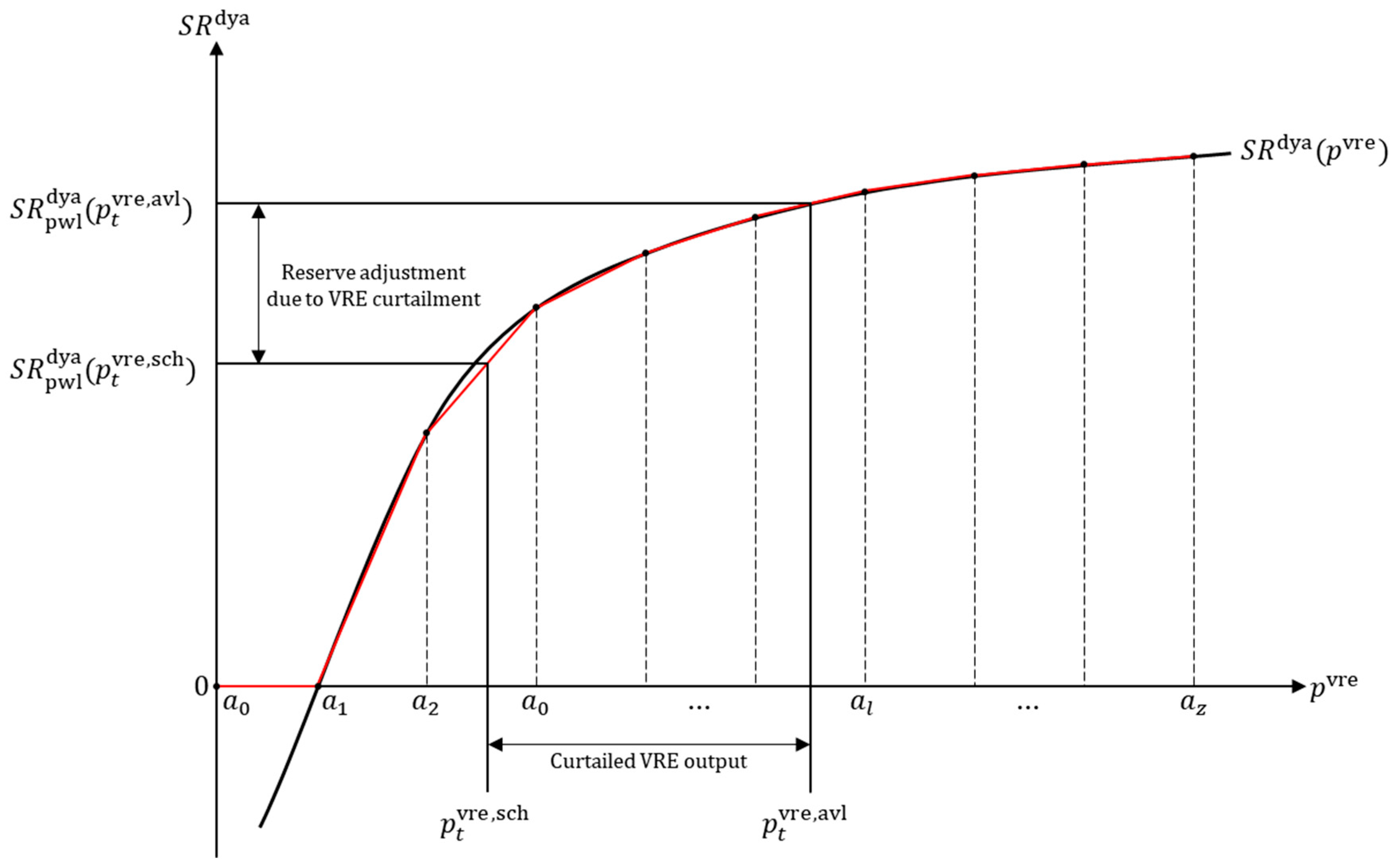
To embed the nonlinear dynamic component of the reserve requirement in a mixed-integer linear programming (MILP) formulation, we approximate it by a piecewise-linear (PWL) function, denoted S R p w l d y a . Specifically, the nonlinear function is evaluated at selected breakpoints over the feasible range of scheduled VRE output, and the function values at adjacent breakpoints are used to construct the linear segments. The PWL form is introduced solely for computational tractability in the MILP. We employ a Big-M-based PWL formulation, depicted in Figure 4 and defined by (2)–(5) [28,29,30,31]. In (4), M denotes a sufficiently large constant.
a l a z a 0 1 λ l , t p t v r e , s c h a l + 1 a z a 0 1 λ l , t ,   l = 0,1 , , z 1
l = 0 z 1 λ l , t = 1 ,           λ l , t { 0 ,   1 }
S R d y a a l + s l p t v r e , s c h a l M 1 λ l , t S R p w l d y a p t v r e , s c h S R d y a a l + s l p t v r e , s c h a l + M 1 λ l , t ,       l = 0,1 , , z 1
s l = S R d y a a l + 1 S R d y a a l a l + 1 a l
The operating reserve requirement formulation developed in this section, including the static/dynamic decomposition in (1) and the PWL approximation in (2)–(5), is incorporated into the RCUC model through the spinning reserve requirement constraints in Section 4.2.7.

4. Formulations

4.1. Objective Function

We assume economic operation of the integrated power and DH systems when electricity and heat are supplied by power- and heat-producing units. Accordingly, we formulate the problem as a mixed-integer linear programming (MILP) model with the objective function in (6), which minimizes the total operating cost of joint power and heat production and determines the optimal operating pattern of each resource. On the power side, the cost components include the fuel and start-up costs of conventional thermal units, as well as penalties for VRE curtailment, while on the heat side, the fuel cost of operating PLBs is considered. To preserve the MILP structure, the quadratic fuel-cost curves of conventional thermal units are approximated by piecewise-linear functions following [27]. In this study, no explicit start-up, shut-down, or degradation cost is assigned to the EB, as these costs are assumed to be small relative to the system-level operating-cost differences examined here.
M i n : t = 1 T i G U { F C i g p i , t g + S C i · u i , t } + n P B F C n p b ( q n , t p b ) + P C · p t v r e , c u r t

4.2. Constraints Considering P2H Technology

We adopt the constraints for nuclear, coal-fired, and gas-fired generators as presented in [27]. Accordingly, this paper describes only the constraints related to CHP, VRE, and the operating reserve requirements.

4.2.1. Electric Power and Heat Balance Constraints

Constraint (7) enforces the power balance condition in the electricity system: in each time t , the sum of generation from all units together with VRE output equals the total electrical demand. When an EB is included as a heat producer, its electricity consumption for heat production is counted on the demand side; likewise, if PSH is modeled, the pumping power used in pumping mode is added to demand. Analogously, constraint (8) imposes the heat-balance condition in the DH system: in each time t , aggregate heat production equals aggregate heat demand, with TES charging treated as demand and discharging treated as supply.
P t l o a d + i P P p i , t p p + m E B p m , t e b = p t v r e , s c h + i G U p i , t g
Q t l o a d + j T S q j , t t s , c / η j t s , c = i C H q i , t g + j T S q j , t t s , d c + m E B q m , t e b + n P B q n , t p b

4.2.2. Variable Renewable Energy Constraints

The scheduled output of VRE units is bounded above by their available output at time t , which is an exogenous input derived from forecasted wind speed and solar irradiance via the corresponding power curves. When required, output may be curtailed.
0 p t v r e , s c h p t v r e , a v l
p t v r e , c u r t = p t v r e , a v l p t v r e , s c h

4.2.3. Combined Heat and Power Plant Constraints

To simplify the model while preserving the routine operating characteristics of CHP plants, the proposed formulation considers only Modes I, III, and V, whereas Modes II and IV are excluded because they correspond to emergency operation. Accordingly, constraints (11)–(14) define the commitment status and operating-mode selection of the CHP unit and, when the unit is online, enforce single-mode operation by requiring that exactly one of these three operating modes be active.
u i , t + d i , t = s i , t s i , t 1
u i , t + d i , t 1
s i , t = s i , t c h p , m 1 + s i , t c h p , m 3 + s i , t c h p , m 5
s i , t c h p , m 1 + s i , t c h p , m 3 + s i , t c h p , m 5 1
The CHP operating characteristics are linearized using a vertex-based representation of the mode-specific feasible power–heat operating region shown in Figure 2. For each mode, the feasible region is modeled as a convex polytope defined by its extreme points, and the CHP operating point is represented as a convex combination of these points, as formalized in constraints (15)–(19) [32].
p i , t g = w = 1 2 h i , w , t m 1 · P i , w m 1 + w = 1 2 h i , w , t m 3 · P i , w m 3 + w = 1 4 h i , w , t m 5 · P i , w m 5
q i , t g = w = 1 2 h i , w , t m 1 · Q i , w m 1 + w = 1 2 h i , w , t m 3 · Q i , w m 3 + w = 1 4 h i , w , t m 5 · Q i , w m 5
w = 1 2 h i , w , t m 1 = s i , t c h p , m 1
w = 1 2 h i , w , t m 3 = s i , t c h p , m 3
w = 1 4 h i , w , t m 5 = s i , t c h p , m 5
As specified by constraints (20) and (21), the CHP unit’s primary and secondary/regulation reserves must be procured within the feasible operating range associated with each operating mode. In standard practice, a unit’s maximum primary reserve is determined by its governor droop, whereas its maximum secondary/regulation reserve is limited by the ramp rate over a 5 min interval [27]. However, for CHP units the reserve capability is mode dependent. In modes that produce electricity and heat simultaneously, some units have reserve provision disabled for plant-stability reasons and therefore provide no operating reserves. Accordingly, constraints (22)–(25) set mode-dependent upper bounds on the primary and secondary/regulation reserves that each unit can provide, consistent with the unit’s operating characteristics.
p i , t g + g r i , t g , u + a g c i , t g , u P i , 2 m 1 · s i , t c h p , m 1 + P i , 2 m 3 · s i , t c h p , m 3 + P i , 3 m 5 · s i , t c h p , m 5
p i , t g g r i , t g , d a g c i , t g , d P i , 1 m 1 · s i , t c h p , m 1 + P i , 1 m 3 · s i , t c h p , m 3 + P i , 1 m 5 · s i , t c h p , m 5
g r i , t g , u G R i , t m 1 , u , m a x · s i , t c h p , m 1 + G R i , t m 3 , u , m a x · s i , t c h p , m 3 + G R i , t m 5 , u , m a x · s i , t c h p , m 5
g r i , t g , d G R i , t m 1 , d , m a x · s i , t c h p , m 1 + G R i , t m 3 , d , m a x · s i , t c h p , m 3 + G R i , t m 5 , d , m a x · s i , t c h p , m 5
a g c i , t g , u A G C i , t m 1 , u , m a x · s i , t c h p , m 1 + A G C i , t m 3 , u , m a x · s i , t c h p , m 3 + A G C i , t m 5 , u , m a x · s i , t c h p , m 5
a g c i , t g , d A G C i , t m 1 , d , m a x · s i , t c h p , m 1 + A G C i , t m 3 , d , m a x · s i , t c h p , m 3 + A G C i , t m 5 , d , m a x · s i , t c h p , m 5
The difference in electric power output between hour t 1 and t of CHP is limited by the ramp rate and expressed by Constraints (26) and (27).
p i , t g p i , t 1 g 60 × R U i
p i , t 1 g p i , t g 60 × R D i
Moreover, CHP units cannot be started up or shut down instantaneously from one hour to the next. Accordingly, we impose minimum up- and down-time constraints, represented by Constraints (28) and (29).
t = k k + M U i 1 s i , t M U i × u i , k
t = k k + M D i 1 1 s i , t M D i × d i , k

4.2.4. Peak Load Boiler Constraints

We account for the feasible operating range of PLBs that produce heat using fossil fuels and expressed by Constraint (30).
Q n , t p b , m i n q n , t p b Q n , t p b , m a x

4.2.5. Electric Boiler Constraints Considering Spinning Reserve

As specified by constraints (31) and (32), the electric boiler’s primary and secondary/regulation reserve contributions must be scheduled within its feasible operating range. The maximum operating reserves available from the EB depend on its technical characteristics. Considering reserve mode operation and thermal equipment stability, this study conservatively assumes that the reserve contribution of the EB is limited to 20% of rated capacity for both reserve categories. Accordingly, constraints (33)–(36) impose upper bounds on the primary and secondary/regulation reserves that the EB can provide. In addition, any temporary reduction in EB heat production associated with reserve activation is assumed to be accommodated within the coupled district-heating system through TES and complementary adjustments of other heat-supply resources under the hourly heat-balance framework.
p m , t e b g r m , t e b , u a g c m , t e b , u P m e b , m a x
p m , t e b + g r m , t e b , d + a g c m , t e b , d P m e b , m i n
g r m , t e b , u G R m , t e b , u , m a x
g r m , t e b , d G R m , t e b , d , m a x
a g c m , t e b , u A G C m , t e b , u , m a x
a g c m , t e b , d A G C m , t e b , d , m a x
We model the heat produced by the electric boiler using an electricity to heat conversion efficiency.
q m , t e b = η m e b · K c o n v e b · p m , t e b

4.2.6. Thermal Energy Storage Constraints

TES charges during surplus periods and discharges when needed. Its operation is bounded by maximum charging and discharging limits, and simultaneous charging and discharging are prohibited. These constraints are given in (38)–(40).
0 q j , t t s , c Q j t s , c , m a x · s j , t t s , c
0 q j , t t s , d c Q j t s , d c , m a x · s j , t t s , d c
s j , t t s , c + s j , t t s , d c 1
TES is subject to a maximum storage capacity. Conversion losses arise during charging and discharging, and standing heat losses occur while energy is stored. These effects are incorporated in constraints (41) and (42), which impose the capacity bound and the intertemporal energy balance with charging/discharging efficiencies and a standing loss term.
C j , t + 1 t s = C j , t t s · 1 f j t s + q j , t t s , c q j , t t s , d c / η j t s , d c
0 C j , t t s C j t s , m a x

4.2.7. Spinning Reserve Requirement Constraints

Constraints (43)–(50) enforce the spinning-reserve adequacy conditions for each time period, requiring that the reserves provided by conventional generators, CHP units, and the electric boiler meet or exceed the corresponding system reserve requirements. The reserve-requirement terms used in these constraints follow the operating reserve requirement formulation introduced in Section 3, specifically the static/dynamic decomposition in (1) and the PWL representation of the dynamic component in (2)–(5).
i G U g r i , t g , u + i P P g r i , t p p , u + m E B g r m , t e b , u S R t G R , u
i G U g r i , t g , d + i P P g r i , t p p , d + m E B g r m , t e b , d S R t G R , d
i G U a g c i , t g , u + i P P a g c i , t p p , u + m E B a g c m , t e b , u S R t A G C , u
i G U a g c i , t g , d + i P P a g c i , t p p , d + m E B a g c m , t e b , d S R t A G C , d
S R t G R , u = S R G R , u , s t a + S R p w l G R , u , d y a ( p t v r e , s c h )
S R t G R , d = S R G R , d , s t a + S R p w l G R , d , d y a ( p t v r e , s c h )
S R t A G C , u = S R A G C , u , s t a + S R p w l A G C , u , d y a ( p t v r e , s c h )
S R t A G C , d = S R A G C , d , s t a + S R p w l A G C , d , d y a ( p t v r e , s c h )

5. Simulation

5.1. Scenarios and Input Data

We simulate a representative winter week in 2030 (168 h), when heat demand is high, to assess the impact of EBs on the Korean power system. The system features high VRE penetration and a large share of inflexible baseload. The following assumptions are adopted.
  • Nuclear units: Because operational flexibility is limited for safety reasons, online nuclear units are operated at rated output for all 168 h and are assumed not to provide operating reserves. This assumption is intended to represent normal scheduling conditions in the Korean power system.
  • CHP units: In modes that produce electricity and heat simultaneously (Modes I and V), equipment characteristics limit rapid and wide adjustments of electric power output. Accordingly, CHP units provide primary reserve only in these cogeneration modes and do not provide secondary/regulation reserve.
  • VRE: For each hour, the available output is determined by wind speed and solar irradiance. At the scheduling stage, the output may be scheduled below the available level (planned curtailment), but we assume VRE units lack real time output control. Therefore, they do not provide operating reserves.
The simulation scenarios used to assess the impact of the EB are organized by the EB’s operating conditions, as summarized in Table 5. Scenario A is the baseline without the EB. Scenario B includes the EB but does not allow it to provide operating reserves. Scenarios C–E evaluate different configurations for reserve provision. In Scenario C, the EB can provide up to 20% secondary/regulation reserve. In Scenario D, it can provide up to 20% primary reserve. In Scenario E, it can provide both services simultaneously.
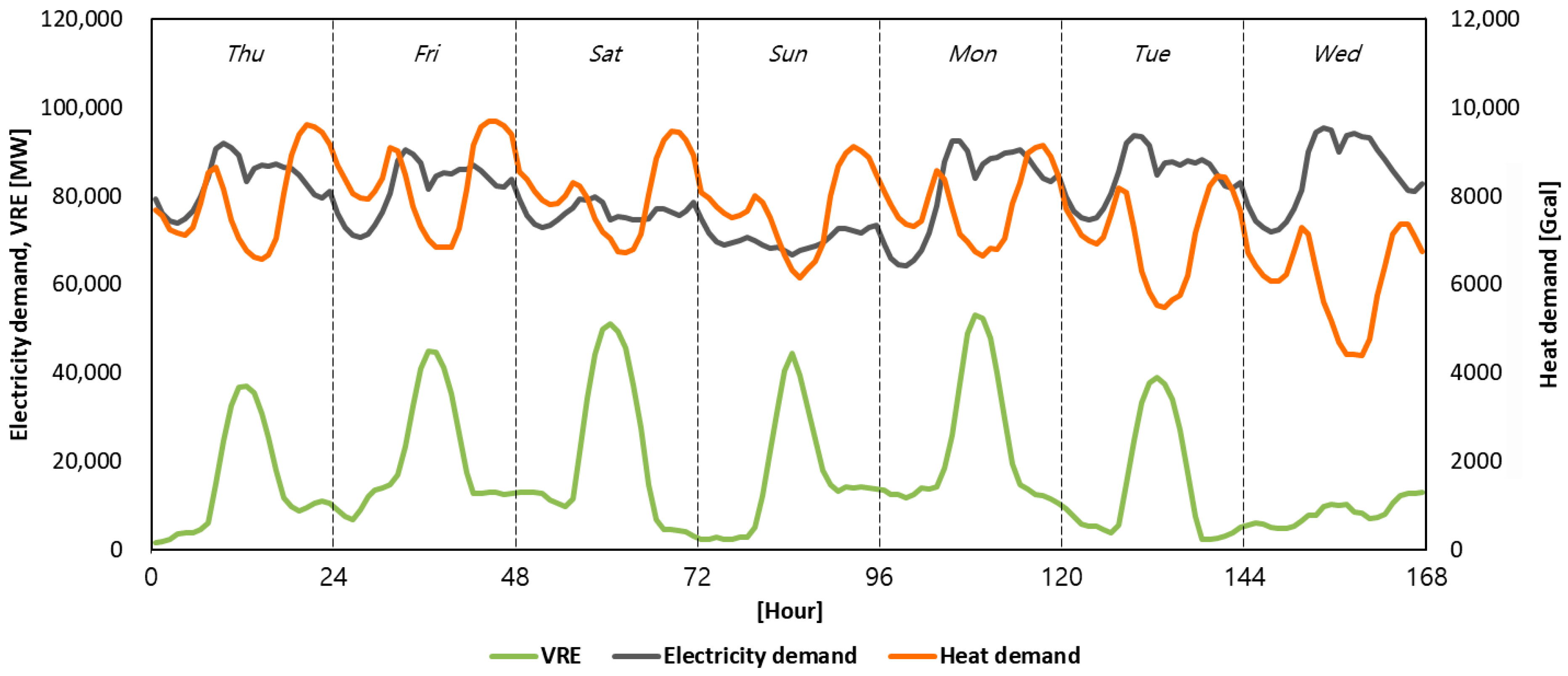
Figure 5 presents the hourly profiles of electricity demand, heat demand, and VRE available output for winter 2030 used in the simulations. Because electricity demand exhibits a weekly cycle, we simulate a single representative week (168 h). To analyze the EB’s impact under high-VRE conditions, we select the winter week with the highest VRE availability. In this study, “VRE output” denotes the available output from wind and solar resources. The 2030 heat-demand profile is projected from the current hourly heat-demand pattern.
The standard deviations σ v r e 1 m p t v r e , s c h and σ v r e 5 m p t v r e , s c h used in the dynamic component of the reserve requirement are given in (51) and (52). The standard deviations in (51) and (52) were obtained using the procedure described in [27], including the generation of weather-based VRE output profiles and the derivation of the corresponding output-dependent variability relationships. In addition, the n-sigma multipliers n v r e 1 m and n v r e 5 m are both set to 1.96, assuming short-term VRE fluctuations are approximately normally distributed.
σ v r e 1 m p t v r e , s c h = 202.57   log 10 p t v r e , s c h + 500 709.12   M W
σ v r e 5 m p t v r e , s c h = 416.72   log 10 p t v r e , s c h + 500 1451.59   M W
The parameter values used in the simulations for the P2H technologies (EB, PLB, TES) are summarized in Table 6.

5.2. Simulation Results

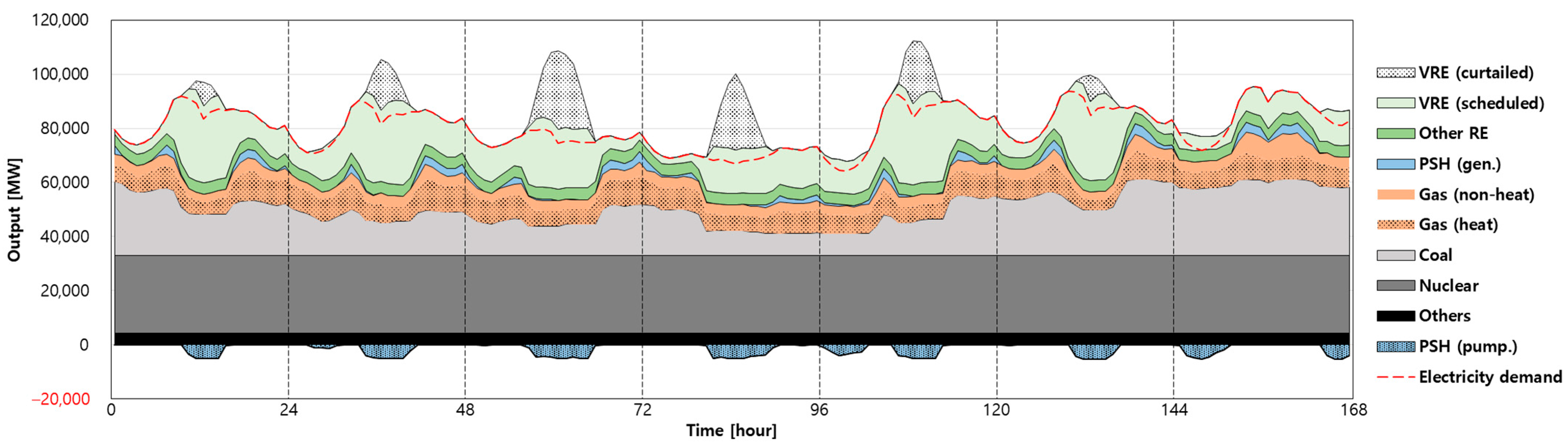
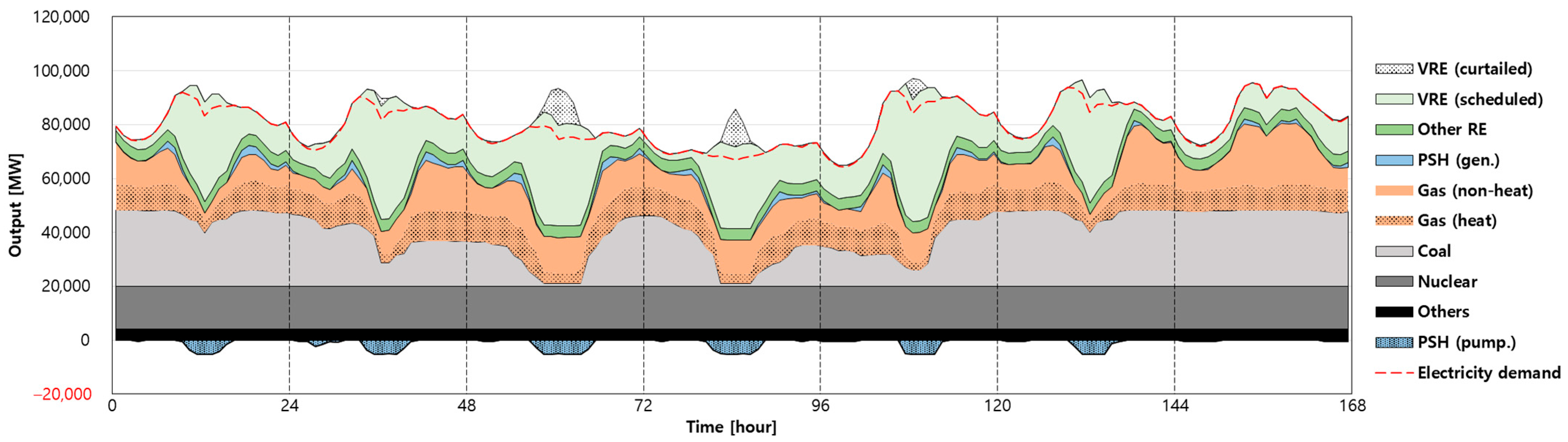
In the simulation results, two cases were compared: one with substantial renewable-energy curtailment (penalty cost of KRW 0/kWh) and one with limited renewable-energy curtailment (penalty cost of KRW 1000/kWh). Figure 6 and Figure 7 present the one-week unit commitment simulation results for Scenario A in winter 2030 under different penalty costs. The figures show the hourly generation by resource. The resource set includes nuclear, coal, gas, PSH, renewable energy (RE), and others category. Gas denotes the electric power output of gas units, including CHP and conventional combined-cycle plants. Gas (heat) denotes the electric power output from CHP when it operates to meet heat demand, that is, the electricity generated concurrently with heat production in cogeneration modes. VRE refers to wind and solar, and the figures also show curtailed VRE. Because PSH in pumping mode and the EB consumes electricity, their electricity consumption is plotted as negative values and thus appears on the demand side.
Table 7, Table 8, Table 9 and Table 10 present the UC simulation results for winter 2030. Table 7 and Table 9 correspond to the case with a penalty cost of KRW 0/kWh, whereas Table 8 and Table 10 correspond to the case with a penalty cost of KRW 1000/kWh. Table 7 and Table 8 report the operating cost by resource for each scenario in billion KRW, and Table 9 and Table 10 report the electricity generation by resource in MWh.
When the penalty cost is KRW 0/kWh, the differences in total operating cost across scenarios are relatively modest because renewable curtailment does not incur an explicit penalty. Relative to Scenario A, Scenario B reduces the total operating cost from KRW 358.26 to 357.63 billion, a decrease of KRW 0.63 billion. Allowing the EB to provide reserves yields additional reductions relative to Scenario B, with total costs of KRW 357.11, 354.18, and 353.80 billion in Scenarios C, D, and E, respectively. In this case, the main effect of the EB is to improve dispatch efficiency and reduce VRE curtailment. Scheduled VRE generation increases from 2,382,048 MWh in Scenario A to 2,458,862 MWh in Scenario E, while curtailed VRE decreases from 446,087 to 369,273 MWh. The benefit is larger when the EB provides primary reserve (Scenarios D and E) than when it provides only secondary/regulation reserve (Scenario C).
When the penalty cost is KRW 1000/kWh, the impact of the EB becomes much more pronounced because reducing renewable curtailment directly lowers both thermal generation and the curtailment penalty. On a cost basis excluding the penalty term, Scenario B lowers the operating cost by KRW 5.35 billion relative to Scenario A, and Scenarios C, D, and E yield further reductions of KRW 2.10, 17.61, and 18.41 billion, respectively, relative to Scenario B. When the penalty term is included, the total cost decreases from KRW 579.51 billion in Scenario A to KRW 566.02 billion in Scenario B, and further to KRW 565.95, 548.14, and 547.23 billion in Scenarios C, D, and E, respectively. Consistent with this trend, curtailed VRE decreases from 91,097 MWh in Scenario A to 82,567 MWh in Scenario E, while gas-fired generation, especially gas (non-heat), declines markedly and lower-marginal-cost resources such as nuclear and VRE account for a larger share of supply. Overall, these results indicate that the operational value of the EB is substantially greater when renewable curtailment is penalized, and that primary-reserve capability provides a much larger system benefit than secondary/regulation reserve alone.
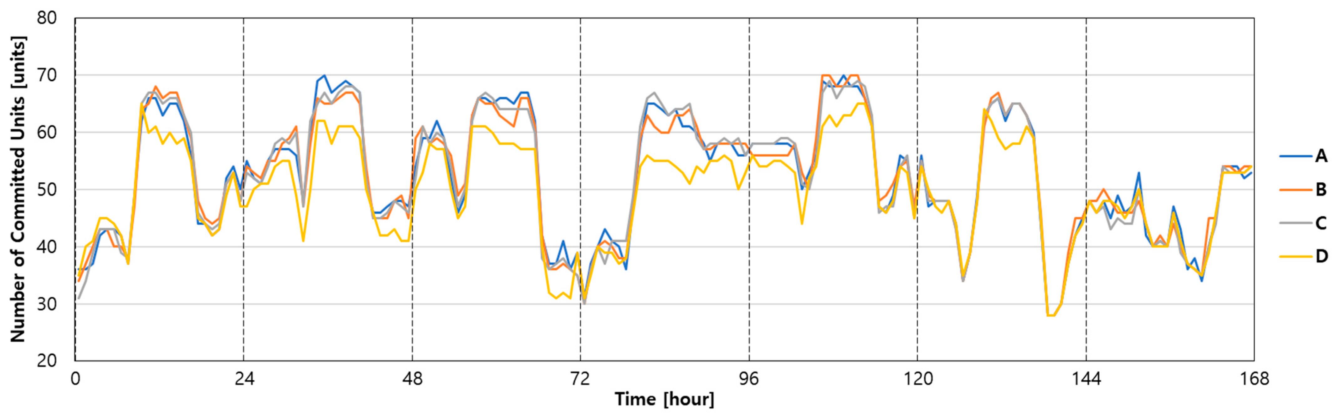
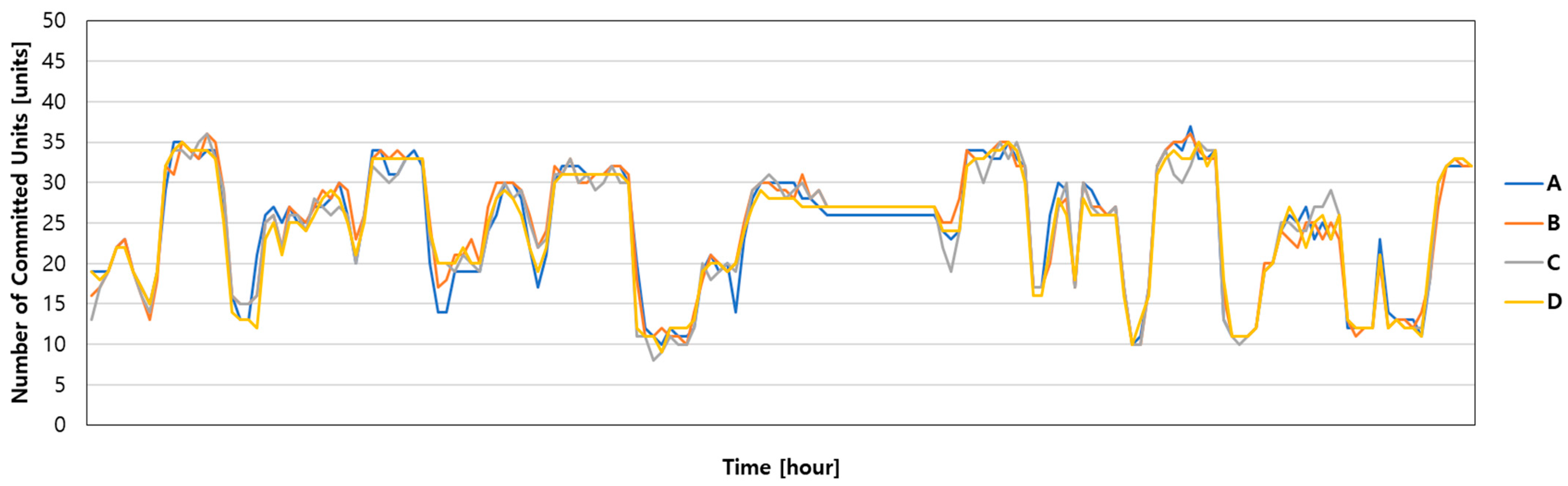
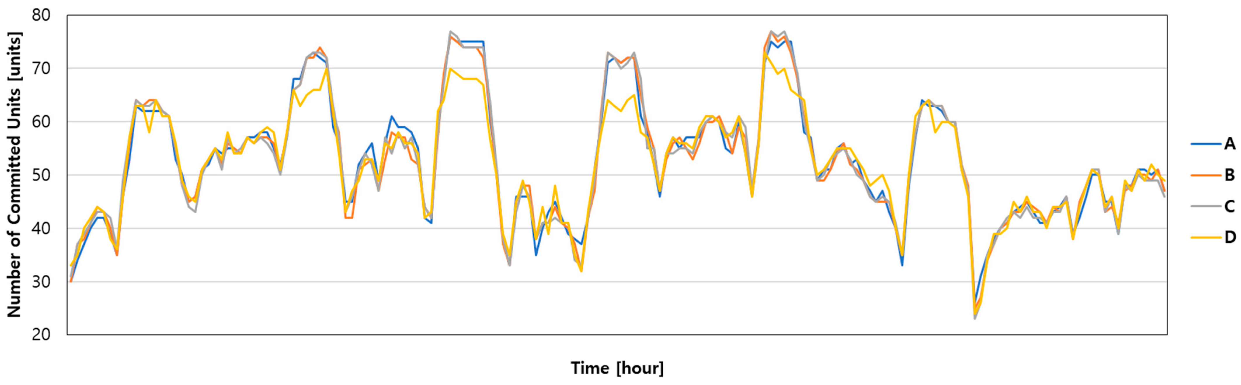
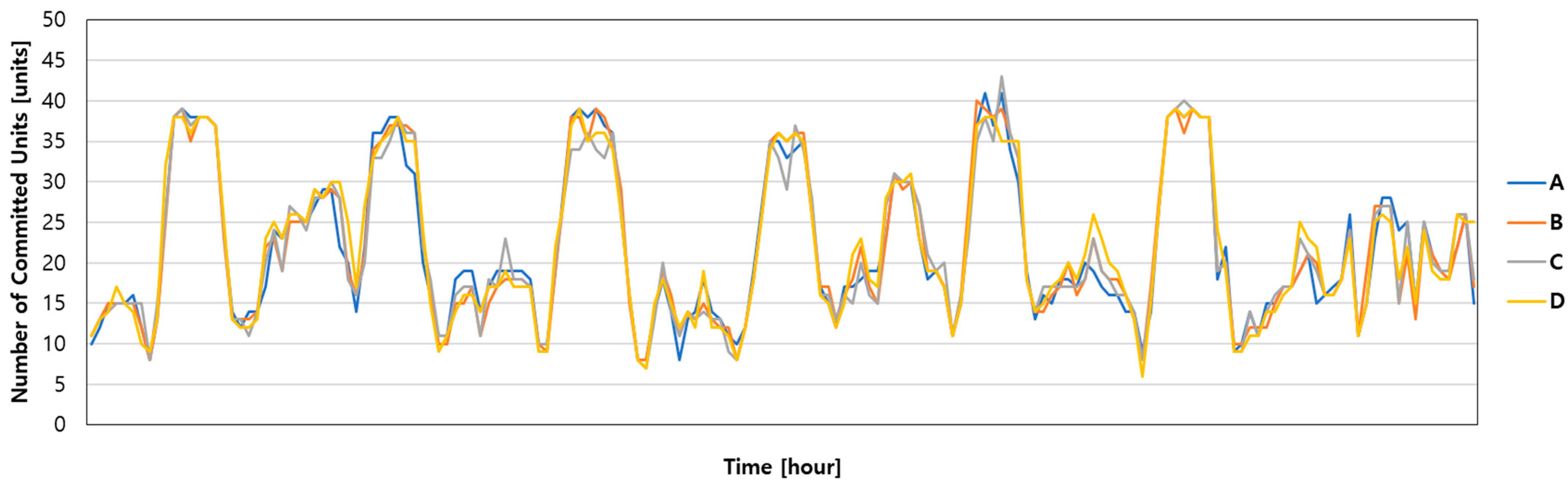
Relative to Scenario A, Scenario B shows that enabling the EB increases electricity demand and mitigates the duck-curve pattern, which in turn can facilitate greater nuclear commitment and/or reduce VRE curtailment, thereby increasing scheduled VRE generation. In Scenarios C, D, and E, the benefit extends beyond duck-curve mitigation: allowing the EB to provide operating reserves reduces the number of conventional thermal units that must remain online solely to satisfy reserve requirements, which creates additional room for lower-marginal-cost resources such as nuclear and VRE. These effects are illustrated in Figure 8, Figure 9, Figure 10 and Figure 11. Figure 8 and Figure 9 correspond to the case with a penalty cost of KRW 0/kWh and show, respectively, the number of committed thermal units required to secure upward primary reserve and upward secondary/regulation reserve. Figure 10 and Figure 11 present the corresponding results for the case with a penalty cost of KRW 1000/kWh. Notably, when the EB is allowed to provide primary reserve, the number of thermal units that must be committed is reduced more substantially than when it provides only secondary/regulation reserve. To highlight the difference between primary reserve provision and secondary/regulation-reserve provision more clearly, Scenario E is excluded from these figures.
This larger benefit of Scenario D than Scenario C arises because EB primary reserve provision more effectively reduces the number of thermal units that must remain online solely to satisfy upward reserve requirements. As a result, the system can avoid part of the inefficient minimum-output or ramping operation of conventional thermal units that would otherwise be committed mainly for reserve procurement.

5.3. Discussion

In this study, the reduction in operating cost under EB operating conditions is primarily associated with lower VRE curtailment and reduced reliance on higher-marginal-cost thermal generation, especially gas. The extent to which dispatch shifts toward nuclear, VRE, and PSH depends on the curtailment-penalty case and the reserve configuration. This result is explained by three factors.
  • During low net load hours, when VRE output is high, the EB increases load and mitigates the duck curve.
  • By providing operating reserves, the EB reduces the number of coal and gas units that need to be committed to meet reserve requirements.
  • Downward reserve provided by the EB reduces the need for other generators to operate above their technical minimum to procure downward reserve, thereby mitigating the increase in their effective minimum output.
As a first factor, comparison of Scenarios A and B shows that enabling the EB increases load during low-net-load hours and mitigates the duck-curve pattern. This additional load relaxes surplus-generation conditions and thereby reduces VRE curtailment. Under the KRW 1000/kWh case, it also allows greater nuclear commitment, whereas under the KRW 0/kWh case the dominant effect is the reduction in curtailment rather than an increase in nuclear output. Accordingly, the additional EB load improves system operation by creating more room for lower-marginal-cost resources, although the exact resource mix depends on the system constraints and the curtailment-penalty assumption.
As a second factor, allowing the EB to provide operating reserves reduces the required number of must-run units needed to meet reserve requirements, which increases nuclear commitment and VRE generation. This effect is evident when comparing Scenarios B, C, D, and E. This mechanism should be distinguished from the direct load-increase effect observed when comparing Scenario B with Scenario A. Whereas the A–B comparison mainly reflects the effect of additional controllable demand, the additional reduction in curtailment across Scenarios C–E arises mainly because fewer thermal units must remain online solely to satisfy reserve requirements. Low net-load typically coincides with periods of high VRE output. In this study, the dynamic reserve requirement is determined using output-dependent standard-deviation functions obtained using the procedure described in [27]. Because the reserve requirement is defined through these functions, the quantitative results can vary with their functional form. Under different weather data, VRE output profiles, or estimation conditions, the resulting variability relationship may differ, which can in turn change the level of dynamic reserve procurement and the number of thermal units committed to satisfy reserve constraints. When the adopted relationship yields a larger reserve increment over certain output ranges, additional coal and gas units may need to remain online, thereby reducing the room for additional nuclear commitment and VRE scheduling. Conversely, when the reserve increment is smaller over those ranges, this effect is moderated. In the present case study, EB reserve provision reduces the number of must-run units, thereby enabling additional nuclear commitment and higher VRE generation.
Finally, when a generator is online, it must operate at or above its technical minimum output. If the generator provides downward reserves, its operational minimum output increases, which reduces the margin for additional nuclear commitment and VRE generation. If the EB provides downward reserve instead, the increase in generators’ operational minimum output is mitigated. As shown in Supplementary Figure S1, EB power input in Scenarios C, D, and E is lower than in Scenario B. Supplementary Figures S2 and S3 show that, in the hours when EB power input is reduced, the EB is providing operating reserves. This indicates that the EB reduces its power input to provide downward reserves. Therefore, allocating EB capacity to the provision of downward reserves yields greater reductions in operating cost than deploying it solely to increase load for duck curve mitigation.
As a result, allowing the EB to provide operating reserves yields a larger decrease in operating cost, and this additional value becomes much more pronounced when renewable curtailment is penalized. The decrease is greater when the EB provides primary reserve than when it provides secondary/regulation reserve. This is because the amount of primary reserve that a generator can provide is limited. For synchronous generators, the available primary reserve is determined by the governor droop together with the normal frequency standard. In Korea the system frequency is maintained within 60 ± 0.2 Hz under normal conditions. For a ±0.2 Hz deviation, the change in output determined by the governor droop is defined as a generator’s primary reserve, which is about 5 percent of its rated capacity. By contrast, secondary reserve is set by ramping capability and equals the change in output over a five minute interval. With a ramp rate of 3 percent per minute, a generator can vary its output by about 15 percent in five minutes. For the same reserve quantity (MW), more generators must be online to meet primary reserve requirements than to meet secondary reserve requirements. In addition, generators that are online can provide both a primary and secondary reserve. As a result, when the EB provides the same quantity of primary and secondary reserve, the decrease in operating cost is therefore larger in the primary case.

6. Conclusions

P2H offers several advantages for the efficient integration of renewable energy into power systems. Prior studies examining these advantages have mostly analyzed how P2H mitigates the duck curve through demand side load increase, whereas evaluations of its effects when P2H provides operating reserves remain limited. Even when P2H is modeled as providing operating reserves, many studies analyze only one reserve category. Among the papers that consider more than one category, analyses are generally conducted from the DH system perspective, and impacts at the national level are not assessed. Moreover, even where national-level assessments exist, the implications of allowing P2H to provide operating reserves have not been adequately considered. Accordingly, this study analyzes the impacts of P2H on the power system by
  • Conducting a comparative analysis based on Korea’s actual 2030 power system, which features high shares of inflexible baseload generation and VRE;
  • Specifying operating-reserve requirements whose dynamic component is represented by a pre-estimated nonlinear variability function derived from weather-based generation profiles and evaluated at the scheduled VRE output; and
  • Classifying the operating-reserve products that P2H can provide into primary reserve and secondary/regulation reserve.
Accordingly, we simulate a set of scenarios for the winter of 2030 by varying the operating conditions of the EB. Scenario A is the base case used to compare the effects of EB deployment under different conditions. Scenario B represents a case in which the EB cannot provide operating reserves. Scenarios C through E assume different reserve products that the EB can provide. Scenario C allows only secondary/regulation reserve, Scenario D allows only primary reserve, and Scenario E allows both. To examine the sensitivity of the results to the valuation of renewable curtailment, two curtailment-penalty cases, KRW 0/kWh and KRW 1000/kWh, were considered. From these simulations, the key findings are as follows.
  • Under the KRW 1000/kWh curtailment-penalty case, Scenario B reduces the operating cost by KRW 5.35 billion compared to Scenario A on a cost basis excluding the curtailment-penalty term. Compared to Scenario B, operating costs in Scenarios C, D, and E decrease by an additional KRW 2.10, 17.61, and 18.41 billion, respectively. Under the KRW 0/kWh case, the corresponding cost reductions are smaller, but the qualitative trend remains the same.
  • By providing operating reserves, the EB reduces the commitment of generators that would otherwise need to remain online solely to satisfy operating reserve requirements.
  • By providing downward reserve, the EB reduces the need for other units to be dispatched above their technical minimum to meet downward reserve requirements, thereby mitigating increases in their effective minimum output.
Taken together, these results indicate that the system value of the EB arises not only from increasing load and mitigating the duck-curve pattern, but also from substituting for conventional reserve providers and relaxing minimum-output constraints on thermal units. The benefit becomes more pronounced when renewable curtailment is penalized, and it is greater when the EB is allowed to provide primary reserve than when it provides only secondary/regulation reserve.
These findings are particularly relevant to the Korean power system, where isolated-grid operation, high nuclear penetration, and increasing VRE share make reserve procurement and curtailment management especially important. In this context, the present study contributes by explicitly distinguishing and quantifying the different system values of EB participation in primary reserve and in secondary/regulation reserve.
At the same time, the present results should be interpreted in light of the study scope. This study focuses on a representative winter week in 2030. According to Korea’s Basic Plan for Electricity Supply and Demand, the planned share of renewable generation in 2030 is 20%. However, given the continuing policy momentum toward higher renewable penetration, future work should evaluate the effects of P2H under scenarios with higher renewable shares and broader seasonal conditions.
In addition, this study adopts a system-level representation of the coupled power and district-heating systems and does not explicitly model transmission or district-heating network constraints. Accordingly, the results do not capture locational congestion, interregional transfer limits, reserve deliverability constraints, or heat-delivery bottlenecks. In practice, such constraints could reduce the ability of the EB to absorb surplus VRE, provide operating reserves, or supply heat to the required district-heating area. For example, if renewable curtailment occurs in a region from which surplus electricity cannot be fully transferred to the EB location because of transmission congestion or limited interregional transfer capability, the EB may not be able to absorb that curtailed renewable energy as assumed in the present model. Similarly, even when the EB is scheduled as a reserve provider in the system-wide model, congestion may limit the practical accessibility of that reserve to the area where balancing support is actually needed, thereby requiring additional commitment or redispatch of local generators. District-heating network constraints, including pipeline transport limits and spatial delivery bottlenecks, may also prevent the heat produced by the EB from being supplied to the required district-heating area. Under such conditions, the EB dispatch estimated by the present model may be only partially achievable in practice, and the operating-cost savings, reserve-provision effects, and curtailment reductions reported in this study should therefore be interpreted as system-level estimates under unconstrained network conditions.
Incorporating network constraints would require enforcement of regional supply–demand balance and would substantially increase computation time. This would necessitate simplified formulations, although overly simplified models may fail to represent the essential effects of P2H adequately. Accordingly, future research should develop a simplified optimization framework that embeds essential electric and thermal network features while preserving the principal effects of P2H, thereby enabling region-specific assessment with tractable computation.
While the present study evaluates the system-level scheduling value of EB reserve provision under normal operating conditions, the reliability contribution of EB resources under extreme contingency events, such as the unexpected outage of a large nuclear unit, is not quantified explicitly. In this regard, Ref. [3] demonstrated the technical prequalification and real-time performance of electric boilers and heat pumps for participation in FCR, aFRR, and mFRR, which supports the technical plausibility of the reserve representation adopted in this study. However, the present framework focuses on week-ahead reserve procurement and scheduling rather than the realization of forced outages and the ensuing post-contingency system response. Future work could therefore extend the present framework to contingency-oriented reliability assessment and dynamic-response analysis in order to evaluate the backup value of EB resources under extreme events more directly.
In addition, the present formulation does not explicitly account for EB cycling- or reserve-activation-related wear costs; if such costs are non-negligible in practice, the reported economic benefit may be somewhat overstated. Furthermore, the current Korean operating rules do not explicitly recognize transmission connected electric boilers as primary-reserve providers. Therefore, the EB primary reserve cases examined in this study should be interpreted as forward-looking technical scenarios rather than as a direct representation of current market eligibility.

Supplementary Materials

The following supporting information can be downloaded at: https://www.mdpi.com/article/10.3390/en19071766/s1, Figure S1: Hourly EB power input profiles for Scenarios B–E (Penalty cost: KRW 1000/kWh); Figure S2: Hourly primary reserve provision for Scenarios C–E (Penalty cost: KRW 1000/kWh); Figure S3: Hourly secondary and regulation reserve provision for Scenarios C–E (Penalty cost: KRW 1000/kWh).

Author Contributions

Conceptualization, Y.-S.L. and W.-J.K.; methodology, Y.-S.L.; software, Y.-S.L.; validation, Y.-S.L., W.-J.K., S.-H.J. and Y.-H.C.; formal analysis, Y.-S.L., W.-J.K. and S.-H.J.; investigation, Y.-S.L.; resources, Y.-S.L. and S.-H.J.; data curation, Y.-S.L.; writing—original draft preparation, Y.-S.L. and W.-J.K.; writing—review and editing, Y.-S.L., W.-J.K., S.-H.J. and Y.-H.C.; visualization, Y.-S.L.; supervision, Y.-H.C.; project administration, Y.-H.C.; funding acquisition, Y.-H.C. All authors have read and agreed to the published version of the manuscript.

Funding

This work was supported by the Korea Institute of Energy Technology Evaluation and Planning (KETEP) and the Ministry of Trade, Industry & Energy (MOTIE) of the Republic of Korea (No. 20226210100100).

Data Availability Statement

Restrictions apply to the availability of the raw data used in this study. The data were obtained from public-sector energy organizations and are not publicly available due to confidentiality and operational restrictions. Access to these data is subject to the permission of the data providers.

Conflicts of Interest

The authors declare no conflicts of interest.

Nomenclature

  • Sets and indices
GUSet of all generating units
CUSet of CHP generating units, CUGU
PPSet of PSH plants, PPGU
TSSet of TES units
EBSet of P2H units
PBSet of PLB units
TOperation period, index by t
iIndex for generating unit, iCU or GU
jIndex for TES unit, jTS
mIndex for P2H unit, mEB
nIndex for PLB unit, nPB
tIndex for time interval, t = 1, ..., T
wVertex index. In Modes 1 and 3, w ∈ {1, 2}. In Mode 5, w ∈ {1, 2, 3, 4}
lSegment index, l = 0, 1, …, z − 1.
a l PWL   breakpoint   on   the   VRE   output   axis   with   a 0 < a 1 < < a z .
s l Slope of segment l.
zNumber of PWL segments.
MBig-M constant used in the PWL constraints, MW
  • Parameters and functions
F C i g ( · ) Fuel cost function of generating unit i at time t.
F C n p b ( · ) Fuel cost function of PLB unit n at time t.
σ v r e 1 m ( · ) Standard deviation of 1 min VRE output variability as a function of VRE output level, MW.
σ v r e 5 m ( · ) Standard deviation of 5 min VRE output variability as a function of VRE output level, MW.
S R d y a ( · ) Dynamic component of the reserve requirement as a function of VRE output, MW.
S R p w l d y a ( · ) PWL   approximation   of   S R d y a ( · ) , MW.
S R p w l G R , u , d y a ( · ) PWL dynamic component of upward primary reserve requirement as a function of scheduled VRE at time t, MW.
S R p w l G R , d , d y a ( · ) PWL dynamic component of downward primary reserve requirement as a function of scheduled VRE at time t, MW.
S R p w l A G C , u , d y a ( · ) PWL dynamic component of upward secondary/regulation reserve requirement as a function of scheduled VRE at time t, MW.
S R p w l A G C , d , d y a ( · ) PWL dynamic component of downward secondary/regulation reserve requirement as a function of scheduled VRE at time t, MW.
S C i Startup cost of unit i, KRW.
P t l o a d System electricity demand at time t, MW.
Q t l o a d System heat demand at time t, Gcal/h.
P C Penalty cost for VRE curtailment, KRW/kWh.
η j t s , c Charging efficiency of TES unit j, %.
η j t s , d c Discharging efficiency of TES unit j, %.
η m e b Energy-conversion efficiency of EB, %
K c o n v e b Electric-to-heat unit-conversion coefficient.
f j t s Standing heat-loss factor of TES j, %.
n v r e 1 m n-sigma multiplier for 1 min VRE output variability.
n v r e 5 m n-sigma multiplier for 5 min VRE output variability.
P i , w m 1 Electric power at vertex w for CHP unit i in Mode 1, MW.
P i , w m 3 Electric power at vertex w for CHP unit i in Mode 3, MW.
P i , w m 5 Electric power at vertex w for CHP unit i in Mode 5, MW.
Q i , w m 1 Heat at vertex w for CHP unit i in Mode 1, Gcal/h.
Q i , w m 3 Heat at vertex w for CHP unit i in Mode 3, Gcal/h.
Q i , w m 5 Heat at vertex w for CHP unit i in Mode 5, Gcal/h.
R U i Upward ramping rate of CHP unit i, MW/minute.
R D i Downward ramping rate of CHP unit i, MW/minute.
M U i Minimum up-time of CHP unit i, hour.
M D i Minimum down-time of CHP unit i, hour.
Q n , t p b , m a x Maximum heat output of PLB unit n at time t, Gcal/h
Q n , t p b , m i n Minimum heat output of PLB unit n at time t, Gcal/h
Q j t s , c , m a x Maximum charging power of TES unit j at time t, Gcal/h
Q j t s , d c , m a x Maximum discharging power of TES unit j at time t, Gcal/h
P m e b , m a x Maximum electric power input of EB unit m at time t, MW.
P m e b , m i n Minimum electric power input of EB unit m at time t, MW.
C j t s , n a x Energy capacity of TES unit, Gcal.
G R i , t m 1 , u , m a x Maximum upward primary reserve of CHP unit i in Mode 1, MW.
G R i , t m 3 , u , m a x Maximum upward primary reserve of CHP unit i in Mode 3, MW.
G R i , t m 5 , u , m a x Maximum upward primary reserve of CHP unit i in Mode 5, MW.
G R m , t e b , u , m a x Maximum upward primary reserve of EB unit m, MW.
G R i , t m 1 , d , m a x Maximum downward primary reserve of CHP unit i in Mode 1, MW.
G R i , t m 3 , d , m a x Maximum downward primary reserve of CHP unit i in Mode 3, MW.
G R i , t m 5 , d , m a x Maximum downward primary reserve of CHP unit i in Mode 5, MW.
G R m , t e b , d , m a x Maximum downward primary reserve of EB unit m, MW.
A G C i , t m 1 , u , m a x Maximum upward secondary/regulation reserve of CHP unit i in Mode 1, MW.
A G C i , t m 3 , u , m a x Maximum upward secondary/regulation reserve of CHP unit i in Mode 3, MW.
A G C i , t m 5 , u , m a x Maximum upward secondary/regulation reserve of CHP unit i in Mode 5, MW.
A G C m , t e b , u , m a x Maximum upward secondary/regulation reserve of EB unit m, MW.
A G C i , t m 1 , d , m a x Maximum downward secondary/regulation reserve of CHP unit i in Mode 1, MW.
A G C i , t m 3 , d , m a x Maximum downward secondary/regulation reserve of CHP unit i in Mode 3, MW.
A G C i , t m 5 , d , m a x Maximum downward secondary/regulation reserve of CHP unit i in Mode 5, MW.
A G C m , t e b , d , m a x Maximum downward secondary and regulation reserve of EB unit m, MW.
S R G R , u , s t a Static component of upward primary reserve requirement, MW.
S R G R , d , s t a Static component of downward primary reserve requirement, MW.
S R A G C , u , s t a Static component of upward secondary/regulation reserve requirement, MW.
S R A G C , d , s t a Static component of downward secondary/regulation reserve requirement, MW.
  • Variables
λ l , t Segment activation indicator at time t. 1if active, else 0.
u i , t Start-up indicator for unit i at time t. 1 if start-up between t − 1 and t, else 0.
d i , t Shutdown indicator for unit i at time t. 1 if shutdown between t − 1 and t, else 0.
s i , t Commitment status of unit i at time t. 1 if on at time t, otherwise 0.
s i , t c h p , m 1 Mode 1 indicator for CHP unit i at time t. 1 if operating in Mode 1 at time t, else 0.
s i , t c h p , m 3 Mode 3 indicator for CHP unit i at time t. 1 if operating in Mode 1 at time t, else 0.
s i , t c h p , m 5 Mode 5 indicator for CHP unit i at time t. 1 if operating in Mode 1 at time t, else 0.
h i , w , t m 1 Weight for vertex w of the Mode 1 for unit i at time t.
h i , w , t m 3 Weight for vertex w of the Mode 3 for unit i at time t.
h i , w , t m 5 Weight for vertex w of the Mode 5 for unit i at time t.
s j , t t s , c Charging indicator for TES unit j at time t. 1 if charging at time t, else 0.
s j , t t s , d c Discharging indicator for TES unit j at time t. 1 if discharging at time t, else 0.
p i , t g Electric power output of unit i at time t, MW.
p t v r e , s c h Scheduled VRE power at time t, MW.
p t v r e , a v l Available VRE power at time t, MW.
p t v r e , c u r t VRE curtailment at time t, MW.
p i , t p p Pumping input of PSH unit i at time t, MW.
p m , t e b Electric power input of EB unit m at time t, MW.
q i , t g Heat output of CHP unit i at time t, Gcal/h.
q j , t t s , c Heat charged to TES unit j at time t, Gcal/h.
q j , t t s , d c Heat discharged from TES unit j at time t, Gcal/h.
q m , t e b Heat output of EB unit m at time t, Gcal/h.
q n , t p b Heat output of PLB unit n at time t, Gcal/h.
C j , t t s Thermal energy stored in TES unit j at time t, Gcal.
g r i , t g , u Upward primary reserve of CHP unit i at time t, MW.
g r i , t p p , u Upward primary reserve of PSH unit i at time t, MW.
g r m , t e b , u Upward primary reserve of EB unit m at time t, MW.
g r i , t g , d Downward primary reserve of CHP unit i at time t, MW.
g r i , t p p , d Downward primary reserve of PSH unit i at time t, MW.
g r m , t e b , d Downward primary reserve of EB unit m at time t, MW.
a g c i , t g , u Upward secondary/regulation reserve of CHP unit i at time t, MW.
a g c i , t p p , u Upward secondary/regulation reserve of PSH unit i at time t, MW.
a g c m , t e b , u Upward secondary/regulation reserve of EB unit m at time t, MW.
a g c i , t g , d Downward secondary/regulation reserve of CHP unit i at time t, MW.
a g c i , t p p , d Downward secondary/regulation reserve of PSH unit i at time t, MW.
a g c m , t e b , d Downward secondary/regulation reserve of EB unit m at time t, MW.
S R t G R , u Upward primary reserve requirement at time t, MW.
S R t G R , d Downward primary reserve requirement at time t, MW.
S R t A G C , u Upward secondary and regulation reserve requirement at time t, MW.
S R t A G C , d Downward secondary and regulation reserve requirement at time t, MW.

References

  1. Ministry of Trade, Industry and Energy (MOTIE). 11th Basic Plan for Electricity Supply and Demand; MOTIE: Sejong, Republic of Korea, 2025.
  2. ENTSO-E. Study on Power and Heat Sectors: Interactions and Synergies; ENTSO-E Aisbl: Brussels, Belgium, 2023; Available online: https://eepublicdownloads.blob.core.windows.net/public-cdn-container/clean-documents/Publications/Position%20papers%20and%20reports/2023/entso-e_integration_power2heat_230130.pdf (accessed on 4 February 2026).
  3. Iov, F.; Khatibi, M.; Bendtsen, J.D. On the Participation of Power-To-Heat Assets in Frequency Regulation Markets—A Danish Case Study. Energies 2020, 13, 4608. [Google Scholar] [CrossRef]
  4. Sihvonen, V.; Ollila, I.; Jaanto, J.; Grönman, A.; Honkapuro, S.; Riikonen, J.; Price, A. Role of Power-to-Heat and Thermal Energy Storage in Decarbonization of District Heating. Energy 2024, 305, 132372. [Google Scholar] [CrossRef]
  5. Kirkerud, J.G.; Trømborg, E.; Bolkesjø, T.F. Impacts of Electricity Grid Tariffs on Flexible Use of Electricity to Heat Generation. Energy 2016, 115, 1679–1687. [Google Scholar] [CrossRef]
  6. Nielsen, M.G.; Morales, J.M.; Zugno, M.; Pedersen, T.E.; Madsen, H. Economic Valuation of Heat Pumps and Electric Boilers in the Danish Energy System. Appl. Energy 2016, 167, 189–200. [Google Scholar] [CrossRef]
  7. Dimoulkas, I.; Amelin, M.; Levihn, F. District Heating System Operation in Power Systems with High Share of Wind Power. J. Mod. Power Syst. Clean Energy 2017, 5, 850–862. [Google Scholar] [CrossRef]
  8. Trømborg, E.; Havskjold, M.; Bolkesjø, T.F.; Kirkerud, J.G.; Tveten, Å.G. Flexible Use of Electricity in Heat-Only District Heating Plants. Int. J. Sustain. Energy Plan. Manag. 2017, 12, 29–46. [Google Scholar] [CrossRef]
  9. Kontu, K.; Rinne, S.; Junnila, S. Introducing Modern Heat Pumps to Existing District Heating Systems—Global Lessons from Viable Decarbonizing of District Heating in Finland. Energy 2019, 166, 862–870. [Google Scholar] [CrossRef]
  10. Sinha, R.; Bak-Jensen, B.; Radhakrishna Pillai, J.; Zareipour, H. Flexibility from Electric Boiler and Thermal Storage for Multi Energy System Interaction. Energies 2020, 13, 98. [Google Scholar] [CrossRef]
  11. Liu, B.; Li, J.; Zhang, S.; Gao, M.; Ma, H.; Li, G.; Gu, C. Economic Dispatch of Combined Heat and Power Energy Systems Using Electric Boiler to Accommodate Wind Power. IEEE Access 2020, 8, 41288–41297. [Google Scholar] [CrossRef]
  12. Yan, R.; Wang, J.; Huo, S.; Zhang, J.; Tang, S.; Yang, M. Comparative Study for Four Technologies on Flexibility Improvement and Renewable Energy Accommodation of Combined Heat and Power System. Energy 2023, 263, 126056. [Google Scholar] [CrossRef]
  13. Zhang, L.; Ma, C.; Wang, L.; Wang, X. Theoretical Analysis and Economic Evaluation of Wind Power Consumption by Electric Boiler and Heat Storage Tank for Distributed Heat Supply System. Electr. Power Syst. Res. 2024, 228, 110060. [Google Scholar] [CrossRef]
  14. Kim, D.-N.; Lee, J.-W.; Son, S.-Y. Feasibility of Grid Flexibility Provision Using Heat Pump Water Heaters Under Midnight Power Services: A Case of South Korea. IEEE Access 2025, 13, 80695–80704. [Google Scholar] [CrossRef]
  15. Böttger, D.; Götz, M.; Theofilidi, M.; Bruckner, T. Control Power Provision with Power-to-Heat Plants in Systems with High Shares of Renewable Energy Sources—An Illustrative Analysis for Germany Based on the Use of Electric Boilers in District Heating Grids. Energy 2015, 82, 157–167. [Google Scholar] [CrossRef]
  16. Romero Rodríguez, L.; Brennenstuhl, M.; Yadack, M.; Boch, P.; Eicker, U. Heuristic Optimization of Clusters of Heat Pumps: A Simulation and Case Study of Residential Frequency Reserve. Appl. Energy 2019, 233–234, 943–958. [Google Scholar] [CrossRef]
  17. Melo, S.P.; Brand, U.; Vogt, T.; Telle, J.S.; Schuldt, F.; Maydell, K.V. Primary Frequency Control Provided by Hybrid Battery Storage and Power-to-Heat System. Appl. Energy 2019, 233–234, 220–231. [Google Scholar] [CrossRef]
  18. Tan, J.; Wu, Q.; Hu, Q.; Wei, W.; Liu, F. Adaptive Robust Energy and Reserve Co-Optimization of Integrated Electricity and Heating System Considering Wind Uncertainty. Appl. Energy 2020, 260, 114230. [Google Scholar] [CrossRef]
  19. Monie, S.W.; Hesamzadeh, M.R.; Åberg, M. Power-to-Heat on the Reserve Capacity Market—Policy Implications Considering Economic Constraints and Competing Heat Production. J. Renew. Sustain. Energy 2022, 14, 055901. [Google Scholar] [CrossRef]
  20. Javanshir, N.; Syri, S.; Tervo, S.; Rosin, A. Operation of District Heat Network in Electricity and Balancing Markets with the Power-to-Heat Sector Coupling. Energy 2023, 266, 126423. [Google Scholar] [CrossRef]
  21. Magni, C.; Quoilin, S.; Arteconi, A. Evaluating the Potential Contribution of District Heating to the Flexibility of the Future Italian Power System. Energies 2022, 15, 584. [Google Scholar] [CrossRef]
  22. Jin, T. Estimating the Potential of Power-to-Heat (P2H) in 2050 Energy System for the Net-Zero of South Korea. Energy 2025, 314, 134206. [Google Scholar] [CrossRef]
  23. Holttinen, H.; Milligan, M.; Kirby, B.; Acker, T.; Neimane, V.; Molinski, T. Using Standard Deviation as a Measure of Increased Operational Reserve Requirement for Wind Power. Wind Eng. 2008, 32, 355–377. [Google Scholar] [CrossRef]
  24. Kim, M.-J.; Song, H.-Y.; Park, J.-B.; Roh, J.-H. Optimization of CHP and Thermal Storage under Heat Demand. In Proceedings of the 2016 12th IEEE International Conference on Control and Automation (ICCA), Kathmandu, Nepal, 1–3 June 2016; pp. 277–281. [Google Scholar] [CrossRef]
  25. Song, H.-Y.; Lee, D.-H.; Roh, J.-H.; Park, J.-B.; Park, Y.-G. Optimal Operation Strategy of Large-Scale CHP in District Heating System. J. Electr. Eng. Technol. 2024, 19, 2843–2858. [Google Scholar] [CrossRef]
  26. Korea Power Exchange (KPX). Power Market Operating Rules (Effective 2 October 2025). Available online: https://www.kpx.or.kr/boardDownload.es?bid=0030&list_no=76043&seq=4 (accessed on 5 February 2026).
  27. Kim, W.-J.; Lee, Y.-S.; Chun, Y.-H.; Jeong, H.-S. Reserve-Constrained Unit Commitment Considering Adjustable-Speed Pumped-Storage Hydropower and Its Economic Effect in Korean Power System. Energies 2022, 15, 2386. [Google Scholar] [CrossRef]
  28. Padberg, M. Approximating Separable Nonlinear Functions via Mixed Zero-One Programs. Oper. Res. Lett. 2000, 27, 1–5. [Google Scholar] [CrossRef]
  29. Croxton, K.L.; Gendron, B.; Magnanti, T.L. A Comparison of Mixed-Integer Programming Models for Nonconvex Piecewise Linear Cost Minimization Problems. Manag. Sci. 2003, 49, 1268–1273. [Google Scholar] [CrossRef]
  30. Vielma, J.P. Mixed Integer Linear Programming Formulation Techniques. SIAM Rev. 2015, 57, 3–57. [Google Scholar] [CrossRef]
  31. Lin, M.-H.; Carlsson, J.G.; Ge, D.; Shi, J.; Tsai, J.-F. A Review of Piecewise Linearization Methods. Math. Probl. Eng. 2013, 2013, 101376. [Google Scholar] [CrossRef]
  32. Dantzig, G.B. Linear Programming and Extensions; Princeton University Press: Princeton, NJ, USA, 1963. [Google Scholar]
Figure 1. Simplified schematic structure of the coupled power and district heating system.
Energies 19 01766 g001
Figure 2. Operating ranges for the routinely used CHP modes.
Energies 19 01766 g002
Figure 3. Operating range and reserve margins of an electric boiler (EB).
Energies 19 01766 g003
Figure 4. Piecewise-linear approximation of the dynamic component of the reserve requirement. The red line denotes the piecewise-linear approximation.
Energies 19 01766 g004
Figure 5. Hourly profiles of electricity demand, heat demand, and VRE available output for a winter week in 2030.
Energies 19 01766 g005
Figure 6. UC results of Scenario A: hourly generation by resource over one week (Penalty cost: KRW 0/kWh).
Energies 19 01766 g006
Figure 7. UC results of Scenario A: hourly generation by resource over one week (Penalty cost: KRW 1000/kWh).
Energies 19 01766 g007
Figure 8. Hourly number of committed thermal generating units for upward primary reserve across Scenarios A–D in winter 2030 (Penalty cost: KRW 0 /kWh).
Energies 19 01766 g008
Figure 9. Hourly number of committed thermal generating units for upward secondary/regulation reserve across Scenarios A–D in winter 2030 (Penalty cost: KRW 0 /kWh).
Energies 19 01766 g009
Figure 10. Hourly number of committed thermal generating units for upward primary reserve across Scenarios A–D in winter 2030 (Penalty cost: KRW 1000 /kWh).
Energies 19 01766 g010
Figure 11. Hourly number of committed thermal generating units for upward secondary/regulation reserve across Scenarios A–D in winter 2030 (Penalty cost: KRW 1000 /kWh).
Energies 19 01766 g011
Table 1. Comparison of reserve products considered in prior studies on P2H participation in ancillary-service markets.
Ref.P2H ResourceReserve Product(s)Clarity of Product SpecificationLimitation
[15]EB and TESaFRR-downClearDid not evaluate primary reserve
[16]Residential HP clustersFRR marketPartially clearFRR is mentioned, but the specific product is not further disaggregated; primary reserve was not considered
[17]EBPCR (=FCR)ClearDid not evaluate secondary reserve (aFRR)
[3]EB and HPFCR, aFRR, mFRRVery clearFocused on technical prequalification and performance rather than system-level scheduling or cost assessment
[18]EBupward/downward reserveInsufficiently
specified
Did not sufficiently represent upward/downward reserve product differentiation
[19]HP and TESReserve market participationInsufficiently
specified
Did not disaggregate reserve services by type and Analyzed from the DH-system perspective
[20]EB, HP and TESFCR, FRR, aFRRClearAnalyzed from the DH-system perspective
[4]EB, HP and TESaFRR-down, FCR-NClearAnalyzed from the DH-system perspective
Table 2. Operating reserve requirements for the Korean power system.
Reserve TypeRequirementActivated bySecured for
UpwardRegulation reserve700 MWAGCShort-term load variation
Frequency
restoration
reserve
Primary1000 MWGovernor, ESSLargest unit loss
Secondary1400 MWAGC
Tertiary1400 MWManualReserve restoration
DownwardOperating reserve2000 MWAGC, Manual, etc.Over-generation,
Renewable energy surplus
Regulation reserve1200 MWAGC, Remote set-point
Table 3. Allocation of the incremental operating reserve requirement.
Reserve TypeCurrent
Requirement
Proposed Requirement
UpwardPrimary1000 MW m a x 1000   M W ,   1000   M W + n v r e 1 m · σ v r e 1 m ( p t v r e , s c h )
Secondary1400 MW m a x 2100   M W ,       1400   M W + 700   M W 2 + n v r e 5 m · σ v r e 5 m p t v r e , s c h 2
Regulation reserve700 MW
DownwardRegulation reserve1200 MW m a x 1200   M W ,   1200   M W 2 + n v r e 5 m · σ v r e 5 m ( p t v r e , s c h ) 2
Table 4. Static and dynamic components of operating reserve requirements.
Reserve TypeProposed Requirement
Static ComponentDynamic Component
UpwardPrimary1000 MW m a x 0 ,   n v r e 1 m · σ v r e 1 m ( p t v r e , s c h )
Secondary/Regulation2100 MW m a x 0 ,   700   M W 2 + n v r e 5 m · σ v r e 5 m p t v r e , s c h 2 700   M W
DownwardRegulation reserve1200 MW m a x 0 ,   1200   M W 2 + n v r e 5 m · σ v r e 5 m ( p t v r e , s c h ) 2 1200   M W
Table 5. Scenario description.
ScenarioElectric Boiler
CapacityPrimary ReserveSecondary Reserve
A0 MW--
B1000 MW0%0%
C1000 MW0%20%
D1000 MW20%0%
E1000 MW20%20%
Table 6. Technical parameters of EB, PLB and TES.
Technology
EBPLBTES
Parameters m E B p m e b , m a x = 1000   M W
m E B p m e b , m i n = 0   M W
η m e b = 0.98
m E B p m p b , m a x = 3000   G c a l
m E B p m p b , m i n = 0   G c a l
j T S Q j t s , c , m a x = 2140   G c a l / h
j T S Q j t s , d c , m a x = 2140   G c a l / h
j T S C j t s , m a x = 36,317   G c a l
η j t s , d c = η j t s , c = 0.98
f j t s = 0.02
Table 7. Operating cost by resource for each scenario (Penalty cost: KRW 0/kWh) (billion KRW).
Fuel TypeScenario
ABCDE
Nuclear28.3028.3028.3028.3028.30
Coal158.12160.44158.16157.94156.60
Gas (heat)117.28114.23115.04113.88115.05
Gas (non-heat)54.5654.6655.6054.0653.85
Total
(excl. Penalty cost)
358.26357.63357.11354.18353.80
Penalty cost0.000.000.000.000.00
Total
(incl. Penalty cost)
358.26357.63357.11354.18353.80
Table 8. Operating cost by resource for each scenario (Penalty cost: KRW 1000/kWh) (billion KRW).
Fuel TypeScenario
ABCDE
Nuclear15.1115.3715.5216.9016.90
Coal186.74186.61187.42183.55183.53
Gas (heat)133.77130.61130.91130.28129.82
Gas (non-heat)152.79150.48147.11134.73134.42
Total
(excl. Penalty cost)
488.42483.07480.97465.46464.66
Penalty cost91.1082.9584.9882.6782.57
Total
(incl. Penalty cost)
579.51566.02565.95548.14547.23
Table 9. Electricity generation by resource for each scenario (Penalty cost: KRW 0/kWh) (MWh).
Fuel TypeScenario
ABCDE
Nuclear4,846,8004,846,8004,846,8004,846,8004,846,800
Coal2,932,3632,977,8472,936,6192,937,0502,912,060
Gas (heat)1,280,9781,248,8831,258,1511,252,5311,264,507
Gas (non-heat)670,498671,720679,789667,656664,301
PSH199,456191,590195,836190,626194,633
VRE (scheduled)2,382,0482,408,0642,423,1872,453,8802,458,862
Other RE710,965710,965710,965710,965710,965
Others717,222717,222717,222717,222717,222
Total13,740,33013,773,09213,768,56813,776,73013,769,351
VRE (available)2,828,1352,828,1352,828,1352,828,1352,828,135
VRE (curtailed)446,087420,071404,948374,255369,273
Table 10. Electricity generation by resource for each scenario (Penalty cost: KRW 1000/kWh) (MWh).
Fuel TypeScenario
ABCDE
Nuclear2,662,8002,713,2002,738,4002,973,6002,973,600
Coal3,393,2993,390,0453,407,3723,328,4593,327,844
Gas (heat)1,462,1861,449,4041,446,5201,434,1921,435,768
Gas (non-heat)1,842,3551,816,5021,776,4481,634,6531,630,727
PSH149,219155,453154,578164,110164,980
VRE (scheduled)2,737,0372,745,1842,743,1502,745,4622,745,568
Other RE710,965710,965710,965710,965710,965
Others717,222717,222717,222717,222717,222
Total13,675,08513,697,97513,694,65513,708,66413,706,675
VRE (available)2,828,1352,828,1352,828,1352,828,1352,828,135
VRE (curtailed)91,09782,95184,98582,67382,567
Disclaimer/Publisher’s Note: The statements, opinions and data contained in all publications are solely those of the individual author(s) and contributor(s) and not of MDPI and/or the editor(s). MDPI and/or the editor(s) disclaim responsibility for any injury to people or property resulting from any ideas, methods, instructions or products referred to in the content.