Article

A Distributed Stochastic Optimization Scheduling Method Using Diffusion-TS Generated Scenario for Integrated Energy System


by
Panpan Xia
,
Chen Chen
,
Li Sun
* and
Lei Pan
*
School of Energy and Environment, Southeast University, Nanjing 211189, China
*
Authors to whom correspondence should be addressed.
Energies 2026, 19(7), 1763; https://doi.org/10.3390/en19071763
Submission received: 6 March 2026 / Revised: 29 March 2026 / Accepted: 31 March 2026 / Published: 3 April 2026

Abstract

The optimal dispatch of integrated energy systems (IESs) is strongly affected by uncertainties on both the supply and demand sides. To model wind power uncertainty and embed it into dispatch decision-making, this paper develops a distributed stochastic scheduling method driven by Diffusion-TS-based scenario generation. First, a conditional Diffusion-TS model is developed to generate high-fidelity wind power scenarios from day-ahead forecasts, and a temperature parameter is introduced to balance scenario diversity and fidelity. Second, a distributed stochastic scheduling framework with chance constraints is established, in which the probabilistic constraints are reformulated into a mixed-integer linear programming problem to address source-load fluctuations while preserving subsystem privacy. Third, the block coordinate descent method is used to decompose the system into cooling, heating, and electricity subproblems for iterative solution. Case study results show that the average CRPS of the generated scenarios is 162.16 MW, which is 34% lower than that of the deterministic forecast benchmark. The total cost of distributed deterministic dispatch is 2.8% higher than that of centralized deterministic dispatch, while the total cost of distributed stochastic dispatch is 53.1% higher than that of distributed deterministic dispatch, reflecting the additional economic cost of uncertainty-aware scheduling. Compared with the traditional LHS-Kmeans method, the scenarios generated by Diffusion-TS are closer to the actual wind power output. Although the resulting dispatch cost is higher, the obtained scheduling results are more consistent with realistic wind power conditions. Overall, the proposed method provides a practical technical route for the secure and economical operation of IESs under uncertainty.

1. Introduction

Energy is the foundation of economic development, national security, and social progress [1]. Under the dual pressure of climate change and energy transition, improving renewable energy utilization and promoting low-carbon energy development have become important issues in modern energy systems. In this context, integrated energy systems (IESs), with the characteristics of multi-energy complementarity and coordinated optimization, have gradually become an important means to improve renewable energy accommodation and achieve emission reduction targets [2]. Meanwhile, as a crucial means of exploiting the low-carbon, efficient, and flexible operating potential of IESs, optimal dispatch has important theoretical value and engineering significance [3].
The optimal dispatch of integrated energy systems is strongly affected by uncertainties from both the supply and demand sides, among which the randomness and volatility of wind power output are particularly prominent. How to accurately characterize wind power uncertainty and effectively incorporate it into dispatch decision-making has become a key issue for ensuring secure and economical system operation [4]. Traditional uncertainty handling approaches mainly include robust optimization and stochastic optimization [5]. Among them, stochastic optimization relies heavily on the quality of typical scenario generation. In early studies, scenario generation was mainly carried out on the basis of assumed statistical distributions. Representative approaches included LHS-based sampling, Monte Carlo simulation, and probabilistic models constructed from forecast-error distributions. Han et al. developed an optimal control strategy for a wind–solar hybrid pumped-storage system using a multi-scenario sharing framework, and employed LHS to construct representative wind and photovoltaic output scenarios [6]. Munkhammar studied the probabilistic and scenario-based prediction of solar irradiance using the Markov Chain Mixture (MCM) distribution model, the Persistence Ensemble (PeEn), and climatological methods [7]. Although these methods are relatively straightforward to implement, their effectiveness is strongly constrained by prior distribution assumptions, which makes it difficult to represent the temporal dependence and nonlinear variation of wind power output with sufficient accuracy [8].
Driven by recent advances in deep learning, generative-model-based scenario generation has attracted growing attention. Models such as Generative Adversarial Networks (GANs) and Variational Autoencoders (VAEs) have been successively applied to wind power scenario generation tasks and have achieved promising results. Liu et al. proposed a graph neural network-based adaptive prediction generative adversarial network (GAPGAN) model to accurately predict short-term future scenarios of wind fields [9]. Li et al. proposed a controllable renewable energy generation method based on an improved VAEGAN model [10]. Nevertheless, GAN-based methods may suffer from training instability and mode collapse [11,12], whereas VAE-based methods often generate overly smooth samples with insufficient local detail [13], which limits their suitability for complex time-series generation tasks.
As a new class of deep generative models, denoising diffusion probabilistic models (DDPMs) have shown strong capability in image generation because of their stable training behavior and effective sample generation [14,15,16]. More recently, diffusion-based methods have also been extended to time-series generation [17]. However, existing methods typically employ recurrent neural networks (RNNs) as backbone models, which may lead to limited performance in long-sequence generation and relatively slow inference. Meanwhile, the step-by-step noise perturbation in the diffusion process may disrupt the intrinsic temporal characteristics of time series, such as trend and seasonality, making it difficult for generated sequences to recover the true dynamic patterns [18,19].
To address these issues, Yuan et al. proposed the Diffusion-TS model [20], which significantly improves time-series generation quality by introducing an interpretable season-trend decomposition architecture and a Fourier-domain loss. This model explicitly decomposes the sequence into trend and seasonal components and constrains them separately, while ensuring consistency with real data in the frequency domain. Therefore, Diffusion-TS provides a promising technical basis for high-fidelity wind power scenario generation.
Although accurate uncertainty characterization is a prerequisite for stochastic dispatch, high-quality scenario generation alone is not sufficient to guarantee effective IES operation. An appropriate dispatch framework is also required to incorporate uncertainty information into operational decision-making.
At the level of optimal scheduling, the operating strategy of an integrated energy system directly affects its economic efficiency and reliability. Existing research mainly falls into two paradigms: centralized optimal scheduling and distributed optimal scheduling [21]. Centralized optimal scheduling is based on global system information and aims to minimize the overall operating cost [22]. This method has strong theoretical optimality and can fully utilize global information to achieve multi-energy collaborative optimization. However, in practical engineering applications, integrated energy systems often involve multiple stakeholders, and each stakeholder may be unwilling to fully share sensitive information such as equipment parameters and operating costs due to commercial privacy or data security concerns [23]. This limits the practical deployment of centralized scheduling. Distributed optimal scheduling provides an effective solution to this problem [24]. It decomposes the original problem into several subproblems, and each stakeholder only needs to exchange limited boundary information to achieve collaborative optimization.
Although distributed optimization scheduling has inherent advantages in privacy protection, most existing studies are still based on deterministic scenarios [25]. As a result, the integration of high-quality uncertainty characterization into distributed stochastic scheduling remains insufficient. How to effectively incorporate the probabilistic information of wind power output into a distributed framework while ensuring the coordinated operation of each subsystem under uncertainty remains a key scientific issue to be addressed.
This study investigates the optimal dispatch of integrated energy systems under source-load uncertainty, with emphasis on high-fidelity wind power scenario generation and distributed stochastic scheduling. The main contributions are as follows:
(1)
The original Diffusion-TS framework is extended from general time-series generation to day-ahead-forecast-conditioned wind power scenario generation. By incorporating the day-ahead forecast as conditional information, the proposed method learns the mapping between forecasted and actual wind power output and improves the fidelity of generated scenarios.
(2)
A temperature-controlled reverse sampling strategy is introduced to explicitly regulate the trade-off between scenario diversity and fidelity, so that the generated wind power scenarios can better satisfy the needs of stochastic dispatch.
(3)
A distributed stochastic dispatch framework is developed to integrate the generated wind power scenarios into IES scheduling under wind-power and electric-load uncertainty. Within this framework, the chance constraints are transformed into a tractable mixed-integer linear programming formulation, enabling distributed solution while preserving subsystem privacy.

2. Construction of IES Distributed Optimization Scheduling Model Based on BCD Algorithm

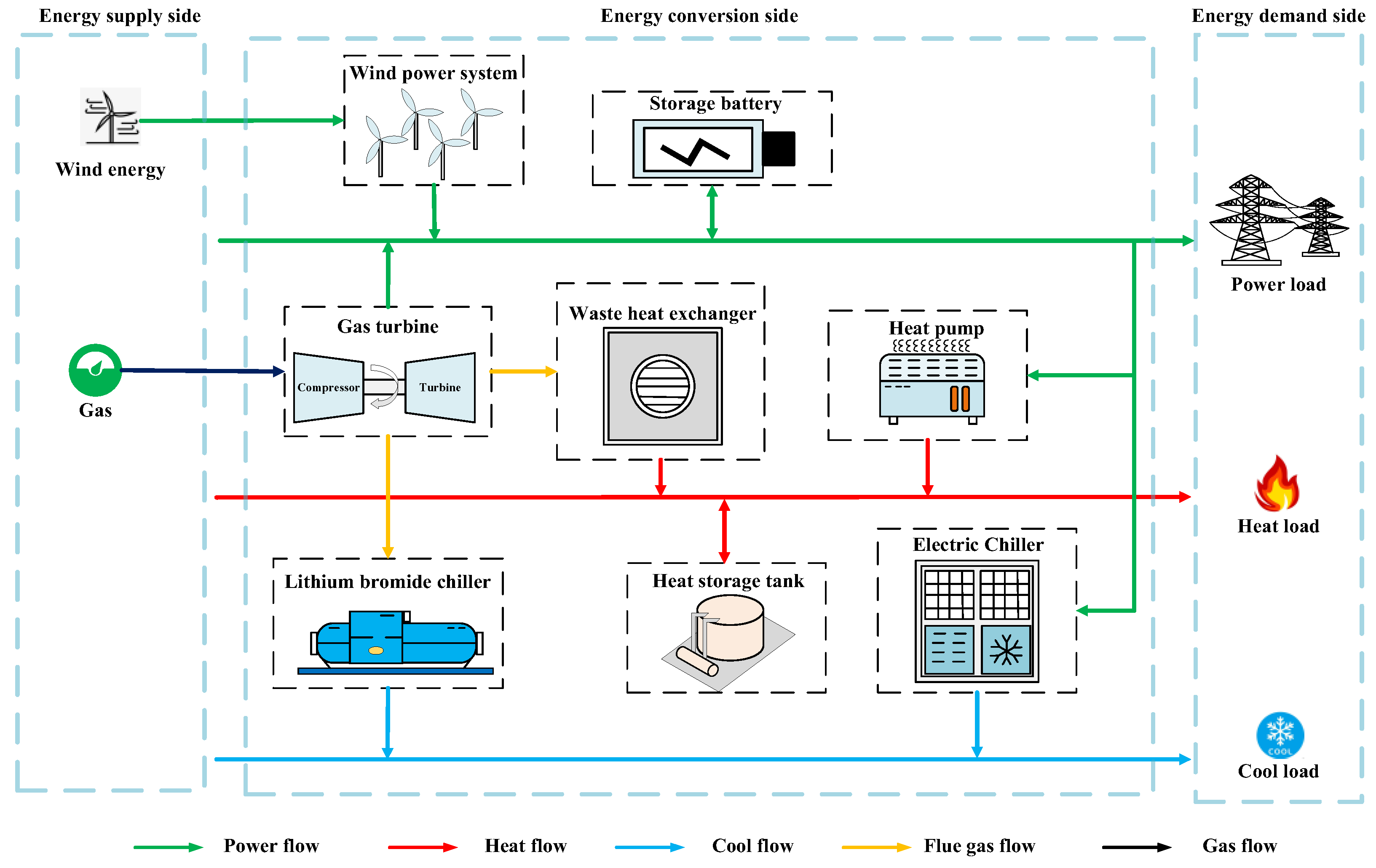
This paper focuses on a typical off-grid combined cooling, heating and power (CCHP) system, as illustrated in Figure 1. The power generation unit of this system consists of wind power units, micro gas turbines and batteries; the heating unit includes heat pumps, heat storage tanks and waste heat exchangers; the cooling unit comprises electric chillers and lithium bromide chillers. The energy flow relationship within the system is illustrated in Figure 1, where the energy coupling relationship is manifested as follows: flue gas can be used for cooling through the lithium bromide chiller and for heating through the waste heat exchanger; the electric chiller relies on electricity for cooling, while the heat pump consumes electricity for heating. Table 1 presents the capacity parameters of each device in this RES.
Based on the above system description, the distributed optimal scheduling model of the integrated energy system is formulated. The model consists of three components: device mathematical models, system constraints, and the objective function. The detailed formulation is presented in the following subsections.

2.1. Steady-State Characteristic Model of CCHP System

(1)
Gas turbine
P t M G T = q N G V t M G T η G T P
Q t M G T = q N G V t M G T η G T H
Equations (1) and (2) describe the electric and thermal outputs of the gas turbine. P t M G T   [kW] and Q t M G T   [kW] represent the electric and thermal outputs at time t; q N G is the calorific value of natural gas, taken as 9.75   kW h / m 3 [26]; V t M G T   [ m 3 ] denotes the natural gas consumption; η G T P , η G T H are the electric and thermal efficiencies, respectively.
(2)
Wind power
P t W T = 0                                                                                         V t V c u t , i n     o r     V t V c u t , o u t P r a t e d W T V t V c u t , i n V r a t e d V c u t , i n                       V c u t , i n V t V r a t e d   P r a t e d W T                                                                                 V r a t e d V t V c u t , o u t  
Equation (3) gives the output model of the wind turbine under different wind speed intervals. In this model, V c u t , i n ,   V r a t e d , V c u t , o u t are the cut-in, rated, and cut-out wind speeds, with their values being 3, 12, and 20 m/s, respectively [27]; V t   [m/s] refers to the actual wind speed at time t; P r a t e d W T   [kW] denotes the rated wind power capacity.
(3)
Heat pump
Q t H P = C O P H P P t H P
Equation (4) expresses the coupling between electric input and heat output of the heat pump. Q t H P   [kW], C O P H P and P t H P   [kW] the heat output, heating coefficient, and electric input, respectively.
(4)
Waste heat exchanger
Q t H E = C O P H E Q t H E , i n
Equation (5) describes the heat conversion relationship of the waste heat exchanger. Q t H E   [ k W ] is the output heat, C O P H E is the heat exchange coefficient of the waste heat exchanger; Q t H E , i n   [kW] is the input heat.
(5)
Lithium bromide chiller
C t A C = C O P A C × Q t A C , i n
Equation (6) describes the lithium bromide chiller. C t A C   [kW] denotes the cooling output of the lithium bromide refrigeration machine; C O P A C is the refrigeration coefficient of the lithium bromide refrigeration machine; Q t A C , i n   [kW] denotes the heat-flow input to the lithium bromide refrigeration machine.
(6)
Electric chiller
C t E C = C O P E C × P t E C
Equation (7) describes the electric chiller, where the cooling output is proportional to its electric input. Here, C t E C   [kW], P t E C   [ k W ] and C O P E C denote the cooling output, electric input, and coefficient of performance, respectively.
(7)
Storage battery
E t E S S = E t 1 E S S + η E S S , c h × P t E S S , c h × z t E S S , c h 1 η E S S , d i s × P t E S S , d i s × z t E S S , d i s
Equation (8) characterizes the energy evolution of the storage battery. E t E S S   [kWh] and E t 1 E S S   [kWh] are the battery energy at time t and time t − 1; η E S S , c h and η E S S , d i s are the charging and discharging efficiencies; P t E S S , c h   [kW] and P t E S S , d i s   [kW] denote the charging and discharging powers; z t E S S , c h and z t E S S , d i s indicate the charging state and discharging state of the battery at time t, which are 0–1 variables.
(8)
Heat storage tank
E t H S = E t 1 H S + η H S , c h × Q t H S , c h × z t H S , c h 1 η H S , d i s × Q t H S , d i s × z t H S , d i s
Equation (9) describes the charging and discharging process of the heat storage tank. E t H S   [kWh] and E t 1 H S   [kWh] represent the stored heat at time t and time t − 1; η H S , c h and η H S , d i s are the charging and discharging efficiencies; Q t H S , c h   [kW] and Q t H S , d i s   [kW] are the charging and discharging thermal powers; z t H S , c h and z t H S , d i s indicates the charging state and discharging state of the heat storage system at time t, which are 0–1 variables.

2.2. Construction of Objective Function and Constraints

According to the energy-flow structure shown in Figure 1, the CCHP system is decomposed into three subproblems, namely cooling, heating, and electricity. In this way, the original centralized scheduling problem is reformulated as a distributed optimization problem and solved by the BCD algorithm. The interactions among subsystems are caused by cross-energy coupling devices, such as the lithium bromide chiller, the electric chiller, and the heat pump.

2.2.1. Sub-Problem of Cold Energy Supply and Demand

(1)
Objective function
Since the cooling subsystem does not involve fuel consumption, its objective is to minimize the operation and maintenance cost of the related devices:
M t o t a l , c = M o m , c = t = 1 T k = 1 K C o m k , c C t k
In Equation (10), C o m k , c represents the operation and maintenance cost coefficient of the k-th device per unit output power in each dispatch interval; C t k is the output power of the k-th device at time t. Because the dispatch interval is 15 min, the original O&M coefficients are converted consistently with t = 0.25 h for cost calculation in each dispatch interval.
(2)
Constraints
The cooling balance constraint is written as:
C t A C + C t E C =   C l o a d t
Here, C l o a d t represents the cooling load demand.
The safety operation constraints of the cold energy sub-problem are as follows:
  γ t k β m i n k , c C r a t e d k C t k γ t k β m a x k , c C r a t e d k
Here, γ t k is the on/off state of device k, where 1 and 0 represent on and off, respectively; β m i n k , c and β m a x k , c are the lower and upper load rates of cold device k; C r a t e d k stands for the rated capacity of the refrigeration equipment, and C t k represents the k-th cold energy subsystem device.

2.2.2. Sub-Problem of Heat Energy Supply and Demand

(1)
Objective function
Similarly, the heating subsystem minimizes the operation and maintenance cost of the involved equipment:
M t o t a l , h = M o m , h = t = 1 T k = 1 K C o m k , h H t k
The symbols have the same meanings as those in the cooling subproblem.
(2)
Constraints
The heat balance constraint is expressed as:
Q t H P + Q t H E + Q t H S , d i s Q t H S , c h = Q l o a d t
Here, Q l o a d t denotes the heating load demand.
In the thermal energy subsystem, we assume that the waste heat flue gas can be discarded:
Q t H E , i n + Q t A C , i n Q t M G T
The safety operation constraints of the thermal energy subsystem are as follows:
γ t k β m i n k , h Q r a t e d k Q t k γ t k β m a x k , h Q r a t e d k
Here, Q r a t e d k represents the rated capacity of the heating equipment, and Q t k represents the k-th thermal energy subsystem equipment; β m i n k , h and β m a x k , h denote the lower and upper load rates of heat device k.
The operating constraints of the heat storage tank are:
β m i n k , h s E r a t e d H S E t H S β m a x k . h s E r a t e d H S 0 Q t H S , c h z t H S , c h Q m a x H S , c h 0 Q t H S , d i s z t H S , d i s Q m a x H S , d i s z t H S , d i s + z t H S , c h 1 E 0 H S = E T H S
Here, E r a t e d H S represents the rated capacity of the heat storage tank. β m i n k , h s represents the minimum state of the heat storage tank; β m a x k . h s represents the maximum state of the heat storage tank.

2.2.3. Sub-Problem of Electricity Supply and Demand

(1)
Objective function
In the short-term dispatching problem, the power subsystem takes fuel cost, equipment operation and maintenance cost, and wind power curtailment penalty as the main objective functions for optimization:
M t o t a l , p = M o m , p + M f u e l + M c u t = t = 1 T k = 1 K C o m k , p P t k + t = 1 T C f u e l V t M G T + t = 1 T C c u t P t W T c u t
In this objective, C o m k , p represents the operation and maintenance cost coefficient of the k-th device per unit output power in each dispatch interval; C f u e l represents fuel cost; C c u t represents wind power curtailment penalty.
(2)
Constraints
The electric power balance constraint is given by:
P t M G T + P t W T + P t E S S , d i s × z t E S S , d i s P t E S S , c h × z t E S S , c h = P t l o a d + P t H P + P t E C + P t W T c u t
The operating constraints of the electricity subsystem are:
γ t k β m i n k , e P r a t e d k P t k γ t k β m a x k , e P r a t e d k
β m i n k , e and β m a x k , e are, respectively, the minimum and maximum load rates of device k; P r a t e d k is the rated electric capacity. γ t k is the corresponding on/off state variable.
The battery operating constraints are written as:
β m i n k , e s s E r a t e d E S S E t E S S β m a x k , e s s E r a t e d E S S 0 P t E S S , c h z t E S S , c h P m a x E S S , c h 0 P t E S S , d i s z t E S S , d i s P m a x E S S , d i s z t E S S , d i s + z t E S S , c h 1 E 0 E E S = E T E E S
Here, E r a t e d E S S represents the rated capacity of the battery. β m i n k , e s s represents the minimum state of the battery; β m a x k . e s s represents the maximum state of the battery.

2.3. The Solution Process of the BCD Algorithm

The Block Coordinate Descent (BCD) method is an iterative algorithm used to solve multi-variable, decomposable optimization problems. Its core idea is to divide the variables in the original problem into several blocks (sub-problems), and in each iteration, fix the variables of other blocks and only optimize the current block’s variables, repeating this process until convergence.
Within the IES distributed optimization model proposed in this paper, the system is decomposed into three subsystems, namely cold, heat, and electricity, each corresponding to a MILP subproblem. After fixing the coupling variables from the other subsystems, each subproblem in the BCD framework still remains a MILP, and the binary variables are updated within each BCD iteration. Therefore, the BCD algorithm is used to decompose the original integrated scheduling problem into three smaller MILP subproblems and solve them iteratively through coupling-variable updates. The implementation steps are shown in Algorithm 1.
Algorithm 1: Block Coordinate Method
Step 1Initialization: Set the iteration count k = 0; set the convergence threshold ε; initialize the variables of each subsystem; cold system C 0 , heat system Q 0 , and power system P 0 .
Step 2Iterative loop (While for convergence): kk + 1
Step 3Fixing the heat and electricity variables, solve the cold energy sub-problem: C ( k ) = a r g m i n c M t o t a l , c   s . t . cold system constraints (update coupling variables: P t E C , Q t C , i n )
Step 4Fixing the cold and electricity variables and solve the thermal energy sub-problem: Q ( k ) = a r g m i n Q M t o t a l , h   s . t . thermal system constraints (update coupling variables: P t H P )
Step 5Fixing the cold and hot variables and solve the sub-problem of electrical energy: P ( k ) = a r g m i n P M t o t a l , P   s . t . the electrical system constraints (update the coupled variables: Q t M G T , Q t H E , i n )
Step 6Calculate the convergence error:
                                                = C k C k 1 + Q k Q k 1 + P ( k ) P ( k 1 )
Step 7Determine convergence:
If < ε , the optimal scheduling scheme is obtained; otherwise, return to step 2.

2.4. Coupling Variables and Privacy-Preserving Mechanism

In the distributed scheduling framework, the cold, heat, and electricity subsystems are coordinated through a limited exchange of coupling variables rather than full sharing of subsystem information. The specific coupling variables exchanged among subsystems are listed in Table 2. Specifically, the exchanged coupling variables include the power demand of the electric chiller and the heat pump, as well as the thermal interaction terms linked to the lithium bromide chiller and the waste heat exchanger. As boundary interaction terms among the three subsystems, they are updated iteratively within the BCD procedure.
It should be emphasized that only the coupling variables are exchanged during the distributed solution process, while the internal parameters of each subsystem, such as equipment capacity limits, operating cost coefficients, and local decision variables, are solved and retained locally. Therefore, the distributed scheduling framework can reduce the need for full information sharing and is more suitable for privacy-preserving coordinated optimization of integrated energy systems.
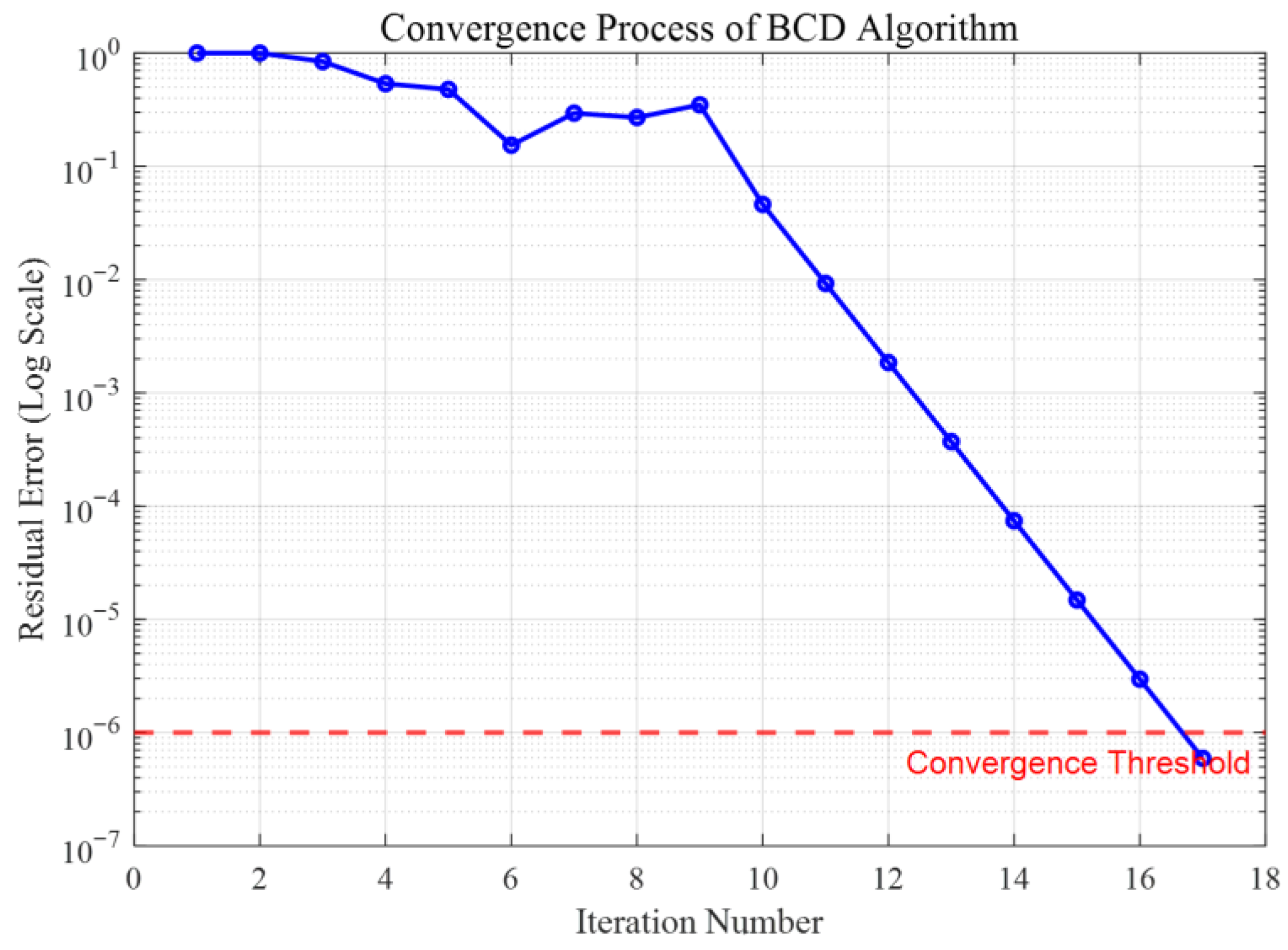
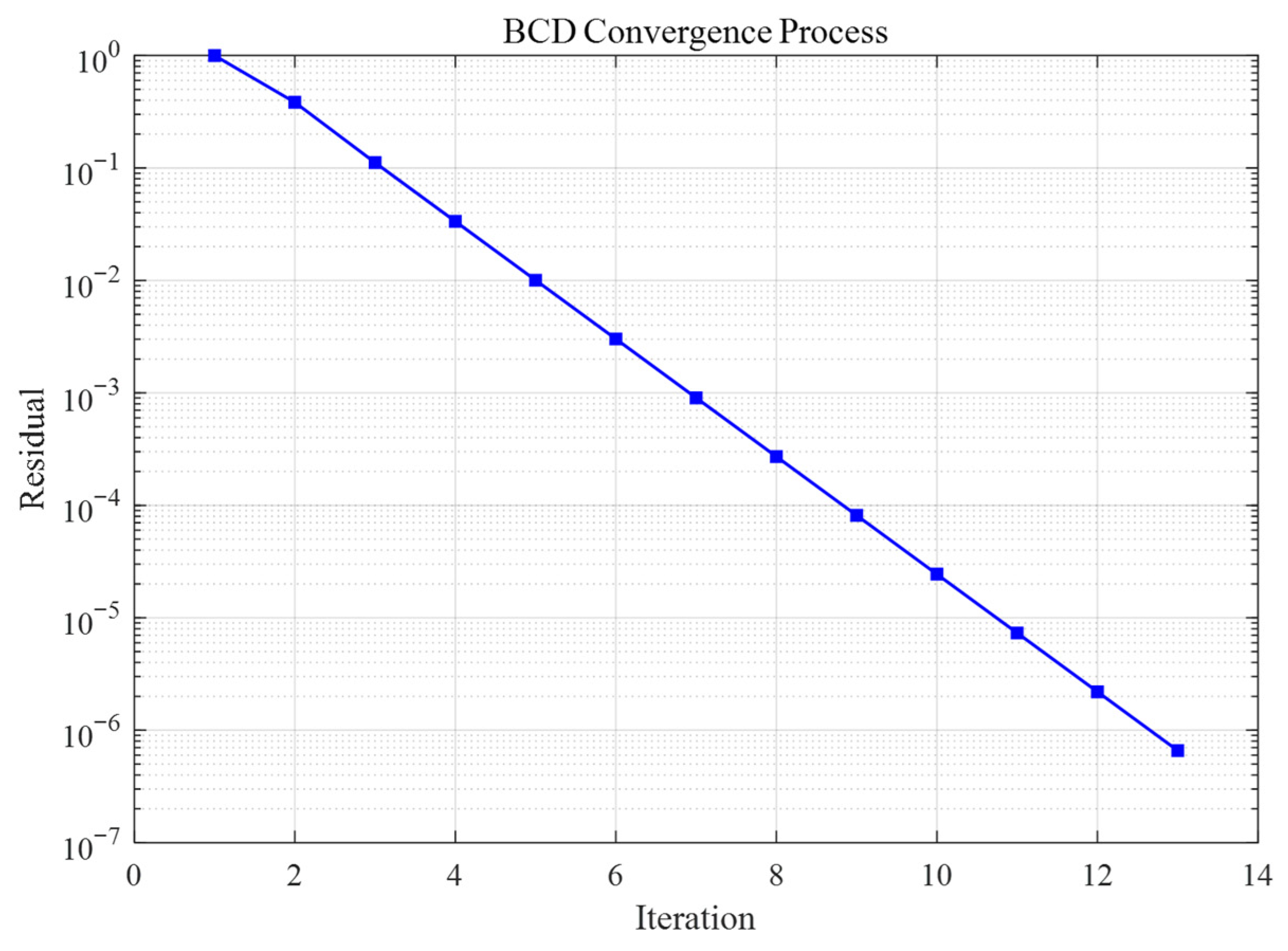
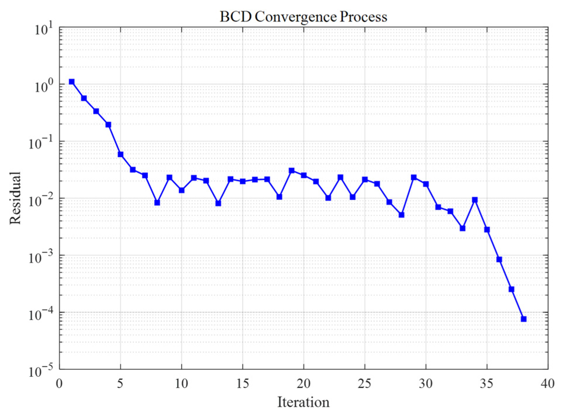
In addition, after fixing the coupling variables from the other subsystems, each subproblem still remains a MILP and is re-solved in each BCD iteration. The convergence curves in Figure 14, Figure 16 and Figure 22 show that the proposed BCD-based distributed framework can achieve stable iterative convergence under the reported problem scale. Together with the scheduling results reported in Section 5, they also provide empirical evidence of its effective coordination capability.

3. Wind Power Scenario Generation Based on the Diffusion-TS Model

3.1. Overview of the Diffusion-TS Model

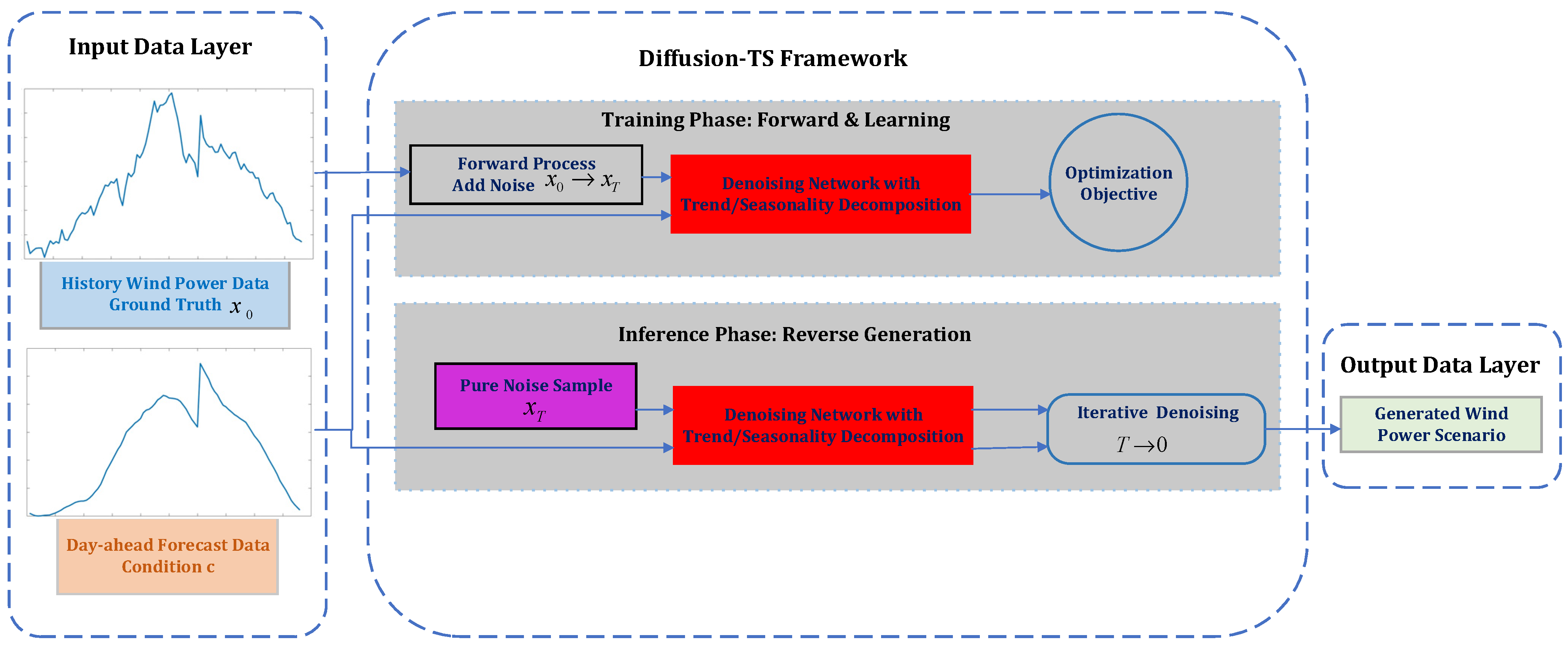
Considering that wind power time series simultaneously exhibit long-term trends and strong short-term random fluctuations, this study adopts the Diffusion-TS framework to generate wind power scenarios. Diffusion-TS is a diffusion-based time-series generation model that can produce diverse multivariate sequences with high fidelity while alleviating the mode collapse problem commonly encountered in generative models. This model is equipped with a built-in seasonal-trend decomposition block, which further separates the sequence into the trend and seasonal components and applies constraints respectively, enhancing model interpretability of generated scenarios. Meanwhile, it introduces a Fourier frequency-domain loss to ensure that its generated scenarios remain consistent with real data in terms of spectral characteristics and to prevent over-smoothing. In addition, the day-ahead forecast sequence is incorporated into the model as conditional information for guiding scenario generation. Through the conditional feature injection mechanism, the model captures the complex mapping from the forecast to the actual output, thereby generating high-confidence scenarios that conform with the historical fluctuation patterns in wind power. The framework of the proposed wind power scenario generation method is shown in Figure 2.

3.2. The Main Structure of the Diffusion-TS Model

3.2.1. The Fundamentals of the Generative Diffusion Framework

The diffusion generation framework consists of two stages, namely a forward noising stage and a reverse denoising stage.
(1)
Forward process
In the forward stage, the original time-series sample x 0 is progressively perturbed by Gaussian noise through a predefined Markov process until it approaches pure noise x T . The corresponding process can be written as follows:
q x t | x t 1 = N x t ; 1 β t x t 1 , β t Ι
Among them, β t 0,1 is the predefined noise scheduling parameter that controls the noise intensity at step t. By using a reparameterization trick and setting α t = 1 β t ,   α ¯ t = s = 1 t α s , any intermediate state x t can be directly sampled from x 0 :
x t = α ¯ t x 0 + 1 α ¯ t ϵ ,             ϵ ~ N 0 , Ι
When T , x T approximately follows a standard Gaussian distribution.
(2)
Reverse process
The reverse stage aims to gradually reconstruct the clean sequence from the noisy sample x T . Different from conventional diffusion models that estimate the added noise, Diffusion-TS is designed to predict the original signal x 0 directly during denoising. Each reverse step is parameterized as follows:
p θ x t 1 | x t = N x t 1 ; μ θ x t , t , Σ θ x t , t
Among them, the mean μ θ x t , t is calculated through the predicted x ^ 0 x t , t , θ (see Equation (8) in [20]), enabling the generation process to more directly utilize the learned data distribution.

3.2.2. Interpretable Decomposition Model Structure

To explicitly model and preserve the complex trend and seasonality patterns in time series, Diffusion-TS introduces a Transformer-based encoder-decoder architecture in the denoising network and integrates an interpretable decomposition layer in the decoder.
(1)
Trend synthesis module
The trend component describes the long-term, smooth changes in the data. Diffusion-TS employs a polynomial regressor to fit this low-frequency behavior:
V t = i = 1 D C · L i n e a r ω t r e n d i , t + X i , t
Here, C = 1 , c , , c p is a polynomial basis matrix composed of the powers of the time index vector c, used to capture the smooth changes in the trend. ω t r e n d i , t is the trend feature vector belonging to the i -th dimension, extracted from the noisy input by the Transformer encoder-decoder network.
(2)
Seasonality and error synthesis module
This module aims to separate periodic components and non-periodic residuals (noise and anomalies) from noisy inputs. Inspired by Fourier series, the model operates in the frequency domain: first, it performs a Discrete Fourier Transform (DFT) on the hidden state ω s e a s i , t representing seasonality. Then, it selects the K frequency components with the largest amplitudes and reconstructs the seasonal signal S i , t through an inverse transformation.
Ultimately, the decoder directly outputs an estimate of the original signal by fusing the trend, seasonal, and residual components:
x ^ 0 x t , t , θ = V t + i = 1 D S i , t + R
Here, R represents the output of the last decoder block, denoting the residual aperiodic component. This decomposition architecture endows each step of the generation process with a clear physical meaning, significantly enhancing the model’s interpretability.

3.2.3. Training Objective: Hybrid Loss Function

L θ = E t , x 0 ω t λ 1 x 0 x ^ 0 2 + λ 2 F F T x 0 F F T x ^ 0 2
Here, ω t represents the time-step related weight, and λ 1 and λ 2 are the coefficients for balancing the two losses. The time-domain loss ensures the accurate reconstruction of data points; the Fourier loss, on the other hand, constrains the generated sequence to maintain consistency with the real data in terms of frequency distribution, which is crucial for capturing the key periodic fluctuation patterns in data such as wind power.

3.2.4. Conditional Generation Mechanism

The original Diffusion-TS model was mainly designed for unconditional generation and interpolation tasks with partial observations. To apply it to wind power scenario generation based on day-ahead forecasts, this paper extends the model to a conditional diffusion model. During the reverse denoising process, the model takes not only the hidden state x t at the current time step and the diffusion step t , but also the day-ahead forecast sequence c as conditional information. The corresponding prediction process can be written as:
x ^ 0 = f θ x t , c , t
In the implemented model, the day-ahead forecast sequence is first encoded into a conditional embedding through a multilayer perceptron and then injected into the denoising Transformer via the adaptive normalization mechanism. In this way, the network can learn the mapping relationship between the day-ahead forecast and the actual wind power output, thereby generating wind power scenarios that better reflect the historical fluctuation characteristics under forecast guidance.

3.2.5. Random Sampling Based on the Temperature Regulation

To precisely adjust the randomness level of the generated scenarios, this paper introduces a temperature parameter τ in the sampling process of the diffusion model. This parameter achieves a trade-off control between the “determinism” and “diversity” of the generated scenarios by scaling the Gaussian noise added during the reverse diffusion process. The sampling step is modified as follows:
x t 1 = μ θ x t , t , c + σ t · τ · z ,             z ~ N 0 , I
Here, μ θ · denotes the denoised mean predicted by the model, σ t   is the theoretical noise standard deviation in the diffusion model at time step t, and τ is the temperature coefficient. When τ = 1, the sampling process strictly adheres to the stochastic definition of DDPM, with the noise amplitude remaining constant. When τ > 1, the effective noise variance increases, which is conducive to enhancing the diversity of the scene and capturing a broader range of possibilities. When τ < 1, the effective noise variance decreases, suppressing randomness and making the generation process more dependent on the conditional information. This may improve the average accuracy but at the expense of diversity.

3.3. Generate Scenario Evaluation Indicators

To evaluate the quality of the generated wind power scenarios, this study uses the Continuous Ranked Probability Score (CRPS) as the main metric and employs the Mean Absolute Error (MAE) as a reference index for deterministic forecasting performance. In addition, the normalized forms, namely nCRPS and nMAE, are introduced to remove the influence of scale and enable more direct comparison.

3.3.1. Continuous Ranked Probability Score

CRPS is used to measure the agreement between the predicted distribution F and the actual observed value y, and can simultaneously evaluate the accuracy of the prediction and the dispersion of the distribution. A smaller value indicates better predictive performance. For an empirical distribution constructed from N generated scenarios, the CRPS at a single time point t is computed as follows:
C R P S t = 1 N i = 1 N x t i y t 1 2 N 2 i = 1 N j = 1 N x t i x t j
Here, N is the number of generated scenarios, and y t is the actual wind power output at time t. x t i and x t j , respectively, denote the predicted output values at time t for the i-th and j-th generated scenarios. The first term in the equation reflects the average absolute error of the generated scenarios, while the second term characterizes the average difference within the scenario set, indicating the degree of dispersion (i.e., diversity) of the distribution. CRPS simultaneously penalizes both the prediction bias and over-dispersion, enabling a comprehensive evaluation of scenario accuracy and the rationality of the corresponding distribution.
As the value of CRPS is affected by the dimension and magnitude of variables, it is difficult to make direct comparisons between different datasets or stations. Therefore, this paper further adopts the normalized CRPS (nCRPS) to eliminate the influence of dimensions:
n C R P S = C R P S M e a n y
Here, Mean(y) represents the mean value of the actual wind power during the observation period.

3.3.2. Mean Absolute Error

To establish a performance benchmark between the generated scenarios and deterministic forecasts, this paper introduces MAE as an evaluation index for the accuracy of point predictions. MAE is defined as:
M A E =   1 T t = 1 T y ^ t y t
Among them, T represents the number of dispatching periods (taken as 96), and y ^ t is the deterministic forecast value at time t. The smaller the MAE, the more accurate the forecast.
Mathematically, when the probabilistic prediction degenerates into a deterministic point prediction, the value of CRPS is exactly equal to MAE. Therefore, comparing the CRPS of the generated scenario set with the MAE of the deterministic forecast has an inherent scale consistency. This comparison not only reflects the central prediction performance of the generated scenarios, but also highlights their ability to describe wind power uncertainty, thereby demonstrating the effectiveness of the proposed deep learning model in improving overall predictive performance.
Similarly, to eliminate the influence of dimensions and facilitate horizontal comparison, this paper normalizes the MAE to obtain the normalized mean absolute error (nMAE):
n M A E = M A E M e a n y × 100 %

4. IES Distributed Stochastic Optimization Scheduling Method Based on Scenario Sampling

Due to the fact that the thermal/cold load has a certain adjustable space, while the electrical load requires a rapid response, this paper only considers the situation where the output of wind power and the electrical load are uncertain. To ensure the operation of the energy system, chance-constrained programming is introduced to characterize the uncertainty of the output of wind power and electric load.

4.1. Chance-Constrained Formulation

In this study, wind power output and electric load are modeled as uncertain variables. Under such source–load uncertainty, it is generally difficult to enforce the electric power balance equality at every time period for all realizations. Therefore, a power imbalance tolerance rate ω is introduced to relax the equality constraint into an allowable interval:
A = P t M G T + P t W T + P t E S S , d i s × z t E S S , d i s B = P t l o a d + P t H P + P t E C + P t W T c u t + P t E S S , c h × z t E S S , c h A 1 ω × B A 1 + ω × B
where A and B denote the total electric power supply and the total actual electric load, respectively.
To further account for uncertainty, the above constraint is reformulated as a chance constraint:
P r A 1 ω × B β P r A 1 + ω × B β
where Pr{·} denotes probability and β is the prescribed confidence level. This formulation requires that the electric power balance remain within the allowable tolerance band with a probability no lower than β, thereby improving the robustness of the scheduling model under uncertain operating conditions.

4.2. Scenario-Based Deterministic Reformulation

Since the chance-constrained model cannot be solved directly by standard linear programming methods, a scenario-based deterministic reformulation is adopted [28]. In this paper, the uncertain wind power is represented by typical scenarios generated by the trained Diffusion-TS model, and the electric load uncertainty is incorporated into the stochastic scheduling framework simultaneously.
Based on the representative scenarios, the original chance constraints are approximated by a deterministic mixed-integer linear programming (MILP) counterpart using binary variables, as shown in Equation (36):
a n , t 0,1 b n , t 0,1 c n , t 0,1 d n , t 0,1   n 1 , N , t 1 , 96   A 1 ω × B L × a n , t 1 ω × B A L × 1 a n , t 1 + ω × B A L × b n , t A 1 + ω × B L × 1 b n , t c n , t = a n , t + b n , t 1 t = 1 96 c n , t 96 L × d n 96 t = 1 96 c n , t L × 1 d n n = 1 N Z n × d n β
Here, L is a very large number, and Z n is the probability of each scenario occurring, satisfying n = 1 N Z n = 1 . Binary variable a n , t is used to indicate whether the total electric power supply of the system in scenario n at time t is not lower than the lower bound of the actual electric load. Binary variable b n , t indicates whether the corresponding supply does not exceed the upper bound of the actual electric load. Accordingly, c n , t reflects whether the electric power balance condition is satisfied within the allowable interval at time t in scenario n. Furthermore, d n is used to represent whether scenario n satisfies the electric power balance requirement over the whole scheduling horizon. Therefore, the chance constraint in this study is imposed in a joint-horizon sense rather than independently at each time period. The last constraint in Equation (36) ensures that the probability of scenarios satisfying the power balance requirement over the entire dispatch horizon is no lower than β .
It should be noted that this reformulation is a finite-scenario approximation, and its effectiveness depends on the representativeness of the generated scenarios. Based on this reformulation, the complete distributed stochastic scheduling model can be solved by the BCD algorithm.

4.3. Overall Framework of the Proposed Stochastic Scheduling Method

The overall IES distributed stochastic optimization scheduling model consists of three main components:
(1) Device mathematical models, including the operational characteristics of generation units, conversion devices, and energy storage systems (Equations (1)–(9));
(2) Objective functions and constraints, including cost minimization, energy balance, and equipment operating limits (Equations (10)–(18), (20) and (21));
(3) Scenario-based deterministic reformulation of chance constraints to handle uncertainties in wind power and load (Equation (36)).
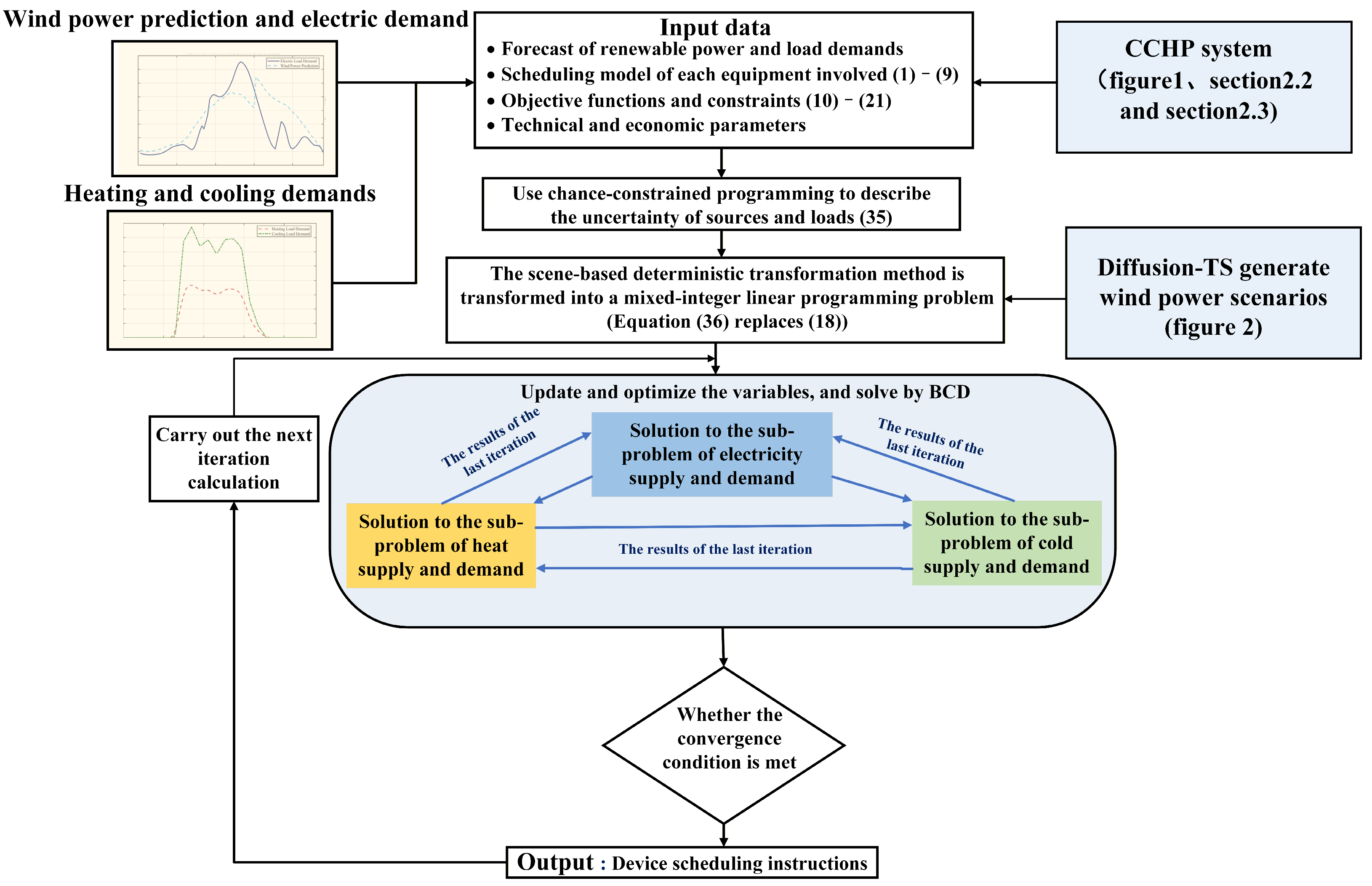
The resulting MILP problem is solved using the block coordinate descent (BCD) algorithm in a distributed manner, where the integrated energy system is decomposed into electricity, heating, and cooling subsystems, and coordination is achieved through iterative updates of coupling variables until convergence. The principle of the method proposed in this study is illustrated in Figure 3.
The Diffusion-TS framework and the optimization framework are coupled through a scenario-based deterministic transformation (see Section 4.2). The Diffusion-TS model generates wind power scenarios to represent the stochastic characteristics of renewable generation, which are then used as inputs to the stochastic optimization model. Based on these scenarios, the optimization framework determines the optimal scheduling strategy of the integrated energy system under uncertainty.
It should also be noted that this study focuses on the optimal scheduling layer of the integrated energy system. The control layer is not explicitly modeled. The obtained scheduling results can serve as reference setpoints or control commands for lower-level control systems.

5. Results and Discussion

5.1. Analysis of Scene Effects Generated by Diffusion-TS

5.1.1. Data Preparation

The case study in this paper is based on day-ahead wind power forecasts and measured wind power data from the Netherlands during 2023–2024. The dataset was collected from the Elia platform, with a sampling interval of 15 min, resulting in 70,176 data points in total. Each sample consists of 96 consecutive points, corresponding to one day. Among them, 584 daily samples are used for model training, and the remaining 147 samples are used for testing. The model is implemented in the PyTorch 2.0.1 environment and trained on an NVIDIA GeForce RTX 4070 Laptop GPU with 16 GB memory, manufactured by NVIDIA Corporation, Santa Clara, CA, USA.

5.1.2. Model Training

For model training, the diffusion process is configured with 500 denoising steps and a cosine noise schedule is adopted to smoothly control the addition and removal of noise. The backbone network is built on a Transformer architecture, where the input sequence length is 96, the hidden feature dimension is 64, and the multi-head attention module contains 4 heads. The encoder and decoder contain 1 and 2 stacked layers, respectively, so as to balance computational efficiency and generation performance. During optimization, the Adam optimizer is employed with an initial learning rate of 1 × 10⁻⁵, together with a warm-up strategy and learning-rate decay. The model is trained for 12,000 epochs, and the loss function is defined as a weighted combination of the L1 loss and a frequency-domain regularization term. Before training, all input data are normalized to the interval [−1, 1].
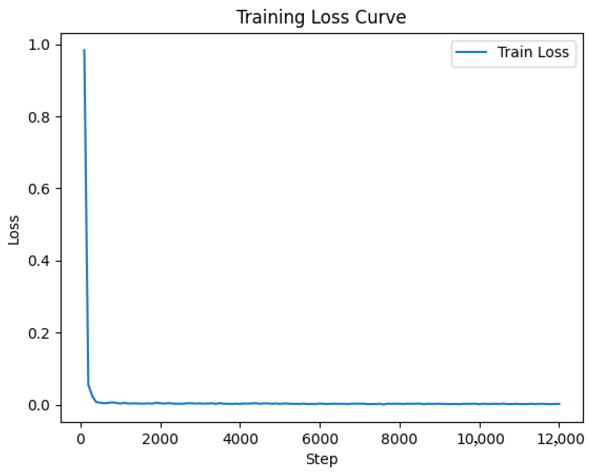
The variation of the training loss is shown in Figure 4. It can be observed that in the initial stage, the value of the loss function drops rapidly, indicating that the model can quickly capture the main trend features in the wind power time series. Subsequently, the curve enters a stable fine-tuning stage with slight fluctuations, during which the model focuses on learning the high-frequency seasonal patterns and random fluctuation details under the Fourier loss constraint. Eventually, the loss curve converges stably without obvious overfitting or oscillation phenomena, suggesting that the training process has good stability.

5.1.3. Analysis of Scenario Generation Effects on the Test Set

(1)
Sensitivity analysis of temperature parameters
The optimal value of τ is determined based on the CRPS metric, which comprehensively evaluates both predictive accuracy and dispersion of the generated scenario set. Specifically, a dedicated sensitivity analysis is conducted, and the τ corresponding to the minimum CRPS value is selected for subsequent scenario generation.
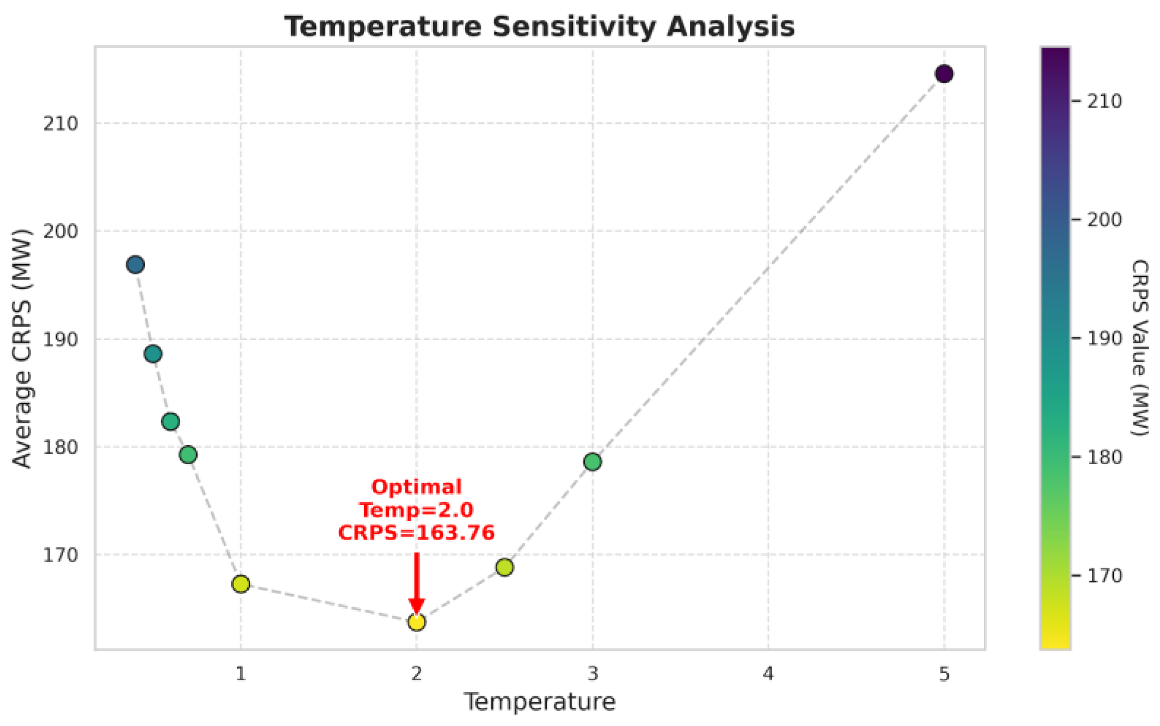
To determine the optimal temperature value τ, a sensitivity analysis was conducted in this paper for τ = 0.4 , 0.5 , 0.6 , 0.7 , 1 , 2 , 2.5 , 3 , 5 , and the results are shown in Figure 5.
Figure 5 shows the changes in the average CRPS evaluation index of the generated scenarios under different temperature parameters. It can be seen that the temperature parameter has a significant impact on the generation quality: both excessively low τ = 0.4 or excessively high τ = 5 temperature values will lead to an increase in the CRPS value. When τ = 2, the model achieves the optimal CRPS value of 163.76 MW, which is approximately 2.1% lower than the benchmark (τ = 1). This indicates that moderate noise injection can enhance the random fluctuations of the generation results, thereby generating a scenario set that is closer to the real wind power probability distribution.
(2)
Analysis of scenario generation results
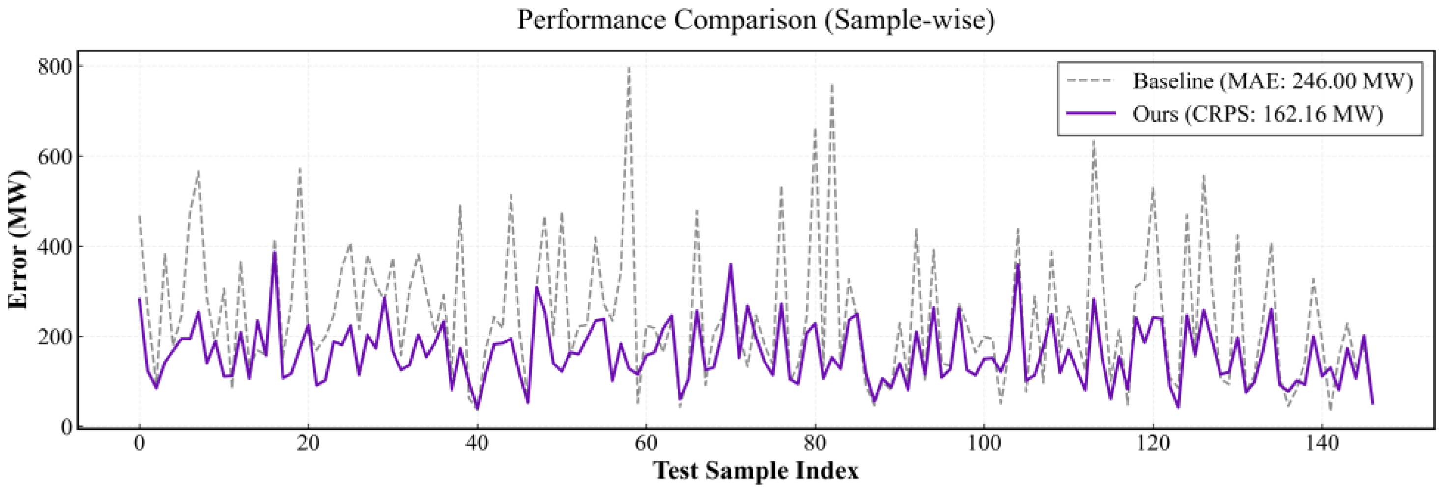
To verify the effectiveness of the Diffusion-TS scenario generation method proposed in this paper, the continuous ranked probability score (CRPS) metric was used to evaluate the generated probabilistic scenarios. As shown in Figure 6, the average CRPS of the model on the test set is 162.16 MW, which is significantly lower than the average absolute error (MAE, 246.00 MW) of the deterministic forecast baseline. Since the CRPS of the deterministic forecast is mathematically equivalent to its MAE, this comparison intuitively demonstrates that the scenario set generated in this study is closer to the actual output distribution than a single point prediction.
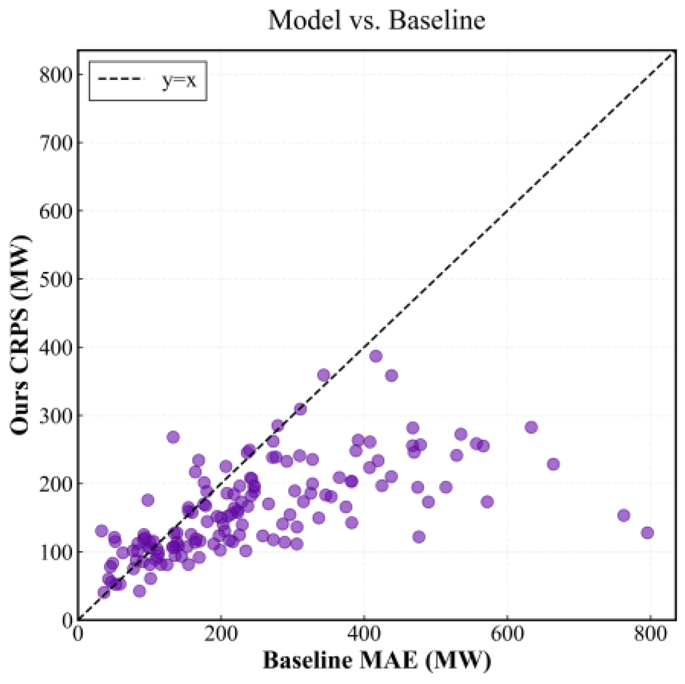
Figure 7 further illustrates the comparison of error distributions of each sample in the test set between the baseline forecast (horizontal axis, MAE) and the scenario generation of Diffusion-TS (vertical axis, CRPS). The dashed line in the figure represents the reference line of equal error, y = x. It can be seen that the vast majority of sample points are densely distributed in the lower right of the reference line (i.e., CRPS < MAE), which fully demonstrates the stable secondary correction ability of the conditional diffusion model for the initial forecast. Additionally, in the high-error range on the horizontal axis (i.e., under the adverse conditions where the baseline forecast has extreme deviations), the scattered points not only do not diverge upwards but also the vertical drop from the reference line further widens. This phenomenon indicates that when the wind power output fluctuates sharply, causing the traditional deterministic forecast to completely fail, the model proposed in this paper can still effectively suppress extreme errors, significantly enhancing the prediction robustness in high-uncertainty scenarios.
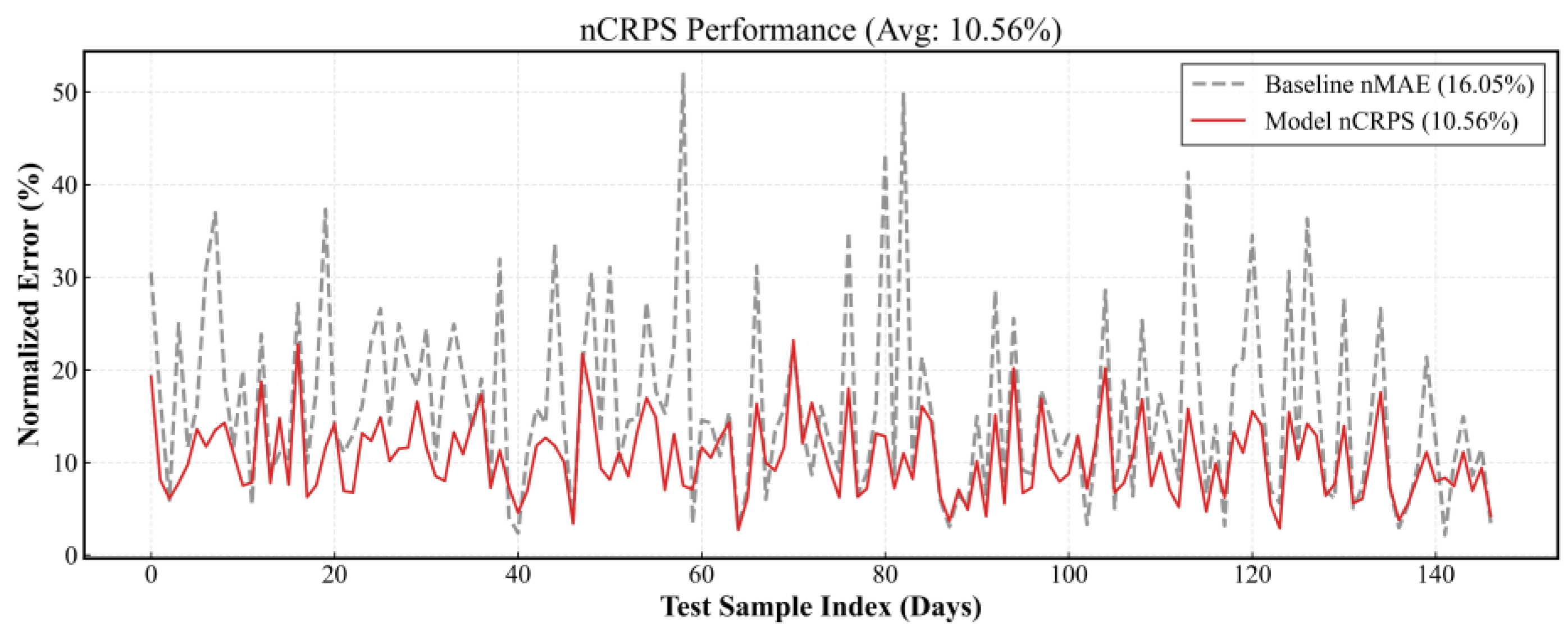
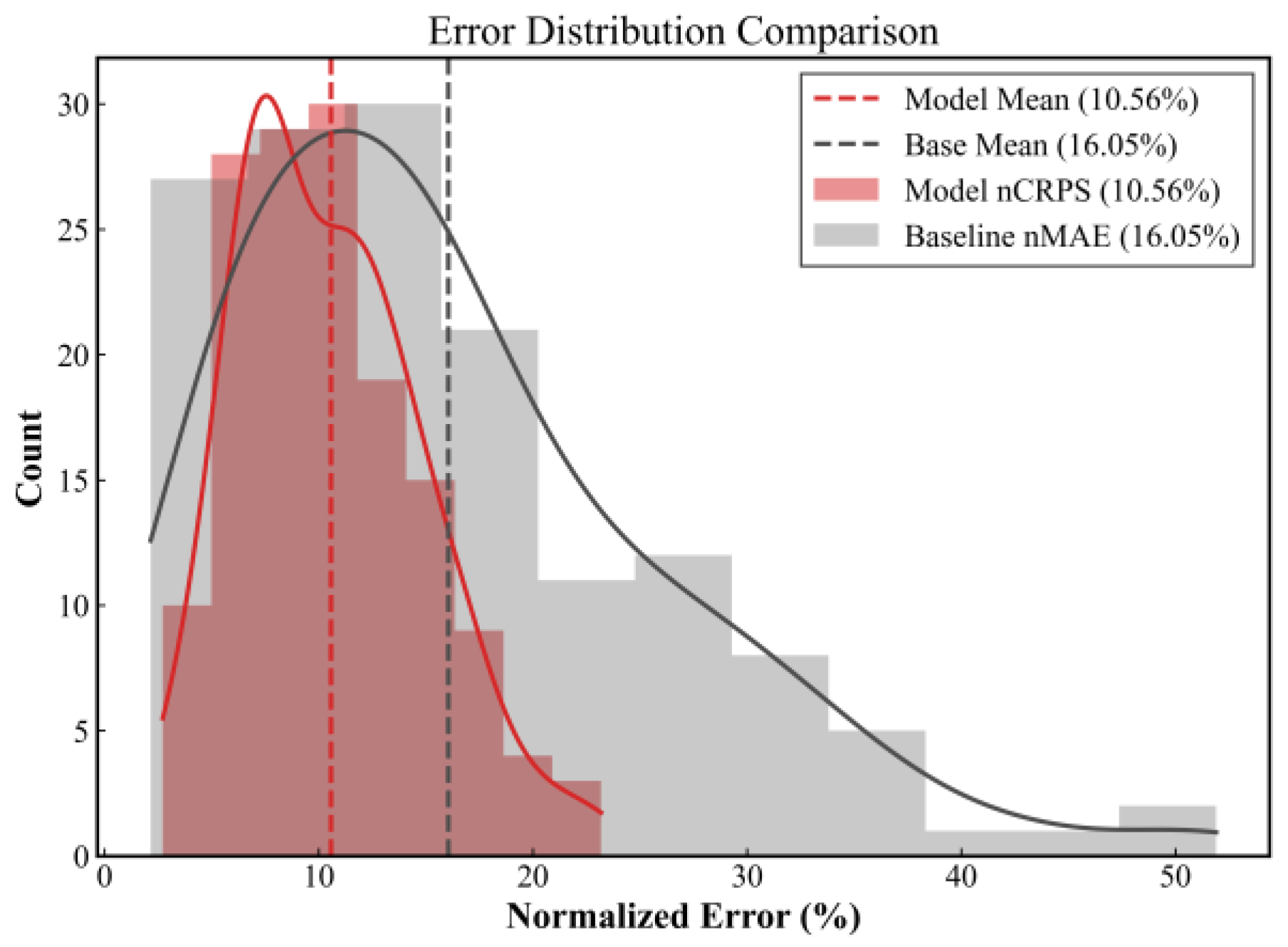
To further eliminate the influence of dimensions and achieve horizontal comparability among data of different scales, this paper adopts the normalized indicators nCRPS and nMAE for supplementary evaluation. As shown in Figure 8 and Figure 9, the average nCRPS obtained by the model is 10.56%, which is better than the 16.05% of the benchmark forecast. The error distribution graph indicates that, compared with the benchmark model, the error distribution of the model in this paper is more concentrated in the low-error range and has a smaller variance. This suggests that the Diffusion-TS model not only improves the prediction accuracy but also more reliably characterizes the randomness of wind power output, providing higher-quality data support for the subsequent distributed stochastic optimization scheduling of the integrated energy system.

5.2. Analysis of Results of BCD Optimization Scheduling Algorithm

5.2.1. Analysis of Scheduling Results

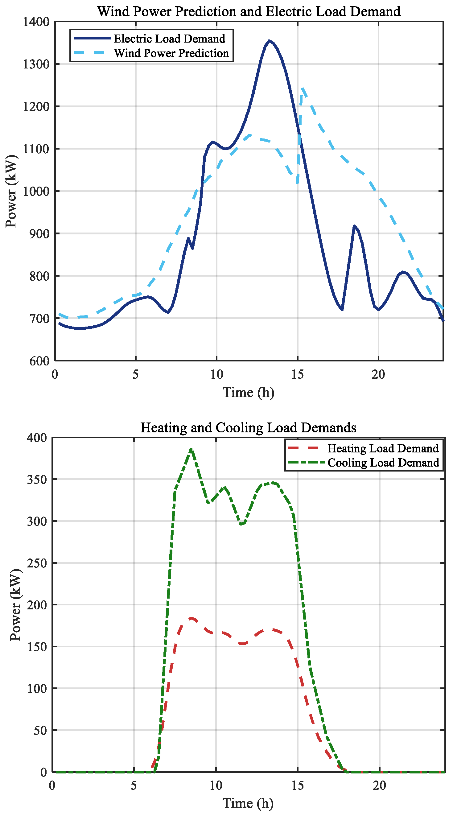
The wind power data is processed by proportional reduction during dispatching, and the variation trends of wind power and electricity, heating, and cooling loads are shown in Figure 10. The load data is obtained from a 30,000 m2 office building. Considering that the load characteristics in spring and autumn are similar, a representative typical day for the spring–autumn season is selected as the basis for dispatching analysis.The dispatching period is 24 h, with a time resolution of 15 min. The economic and technical parameters of the equipment involved in the dispatching are listed in Table 2 and Table 3.
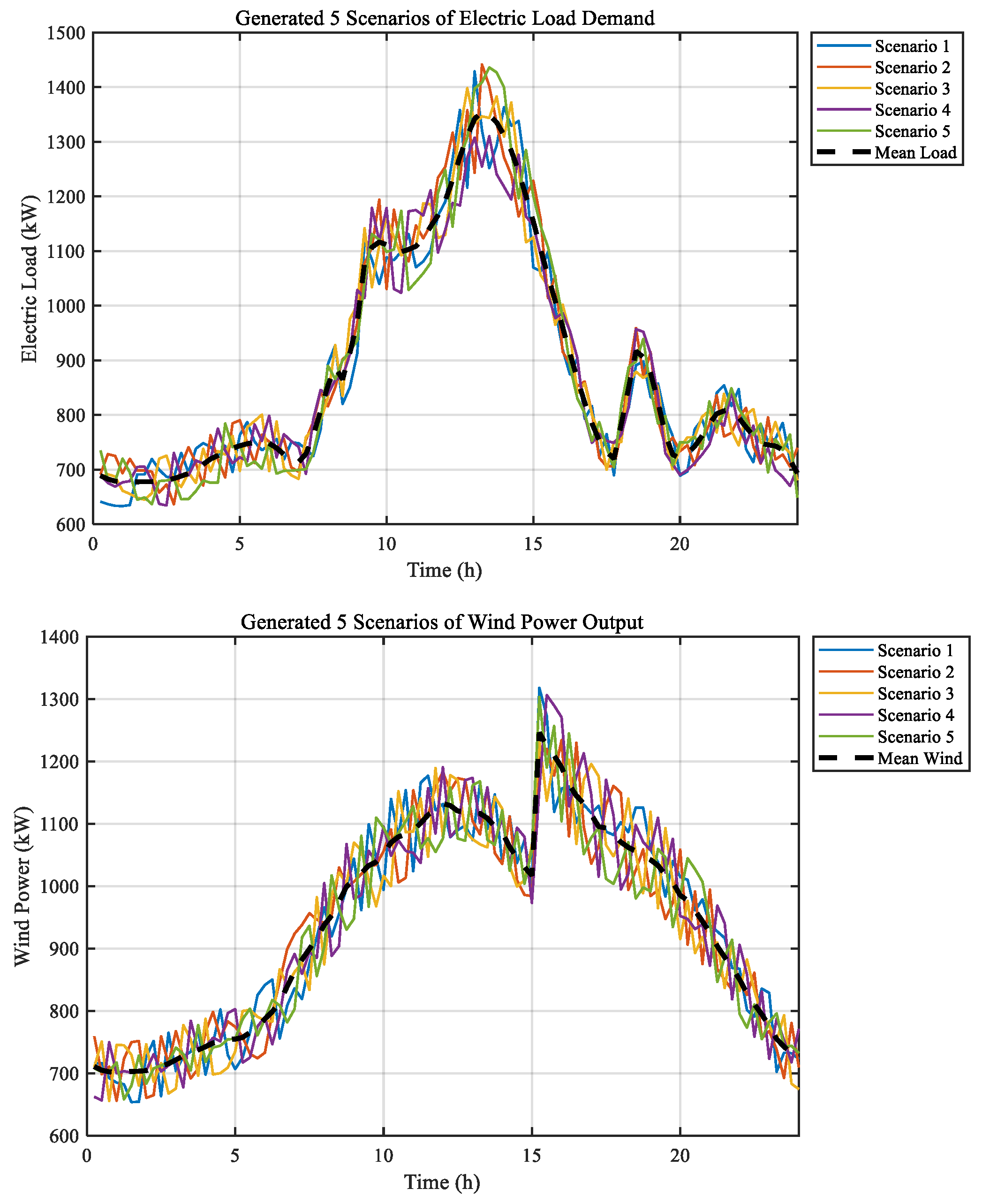
Three comparative cases were set up in the dispatching section: Case 1 is centralized deterministic optimization dispatching, Case 2 is distributed deterministic optimization dispatching, and Case 3 is distributed uncertain optimization dispatching. In Case 3, the number of representative scenarios was set to N = 5, the confidence level was set to β = 0.95, and the power imbalance rate was set to ω = 0. The electric load and wind power output scenario generation curves are shown in Figure 11.
It should be noted that the stochastic dispatch in Case 3 is based on the traditional LHS-Kmeans scenario generation method. Therefore, the economic comparison in this subsection mainly reflects the effects of distributed architecture and stochastic robustness. The impact of replacing the traditional scenarios with Diffusion-TS scenarios is further discussed in Section 5.3.
Table 2. Economic and technical parameters of energy storage equipment [28,29].
EquipmentCharge and Discharge EfficiencyMinimum StateMaximum StateCharge and Discharge Capacity
Power Limit
Initial StateMaintenance Cost Coefficient (¥)
Storage battery0.950.20.950.30.50.0018
Heat storage tank0.900.20.950.50.50.0016
Table 3. Technical and economic parameters of other equipment [28,29].
EquipmentElectrical EfficiencyThermal/Cold EfficiencyMinimum Load RateMaintenance Cost
Coefficient (¥)
Wind turbine0.08
Gas turbine0.340.540.30.0768
Waste heat exchanger0.750.007
Lithium bromide chiller1.20.10.008
Electric chiller4.00.10.0097
Heat pump4.00.10.0097
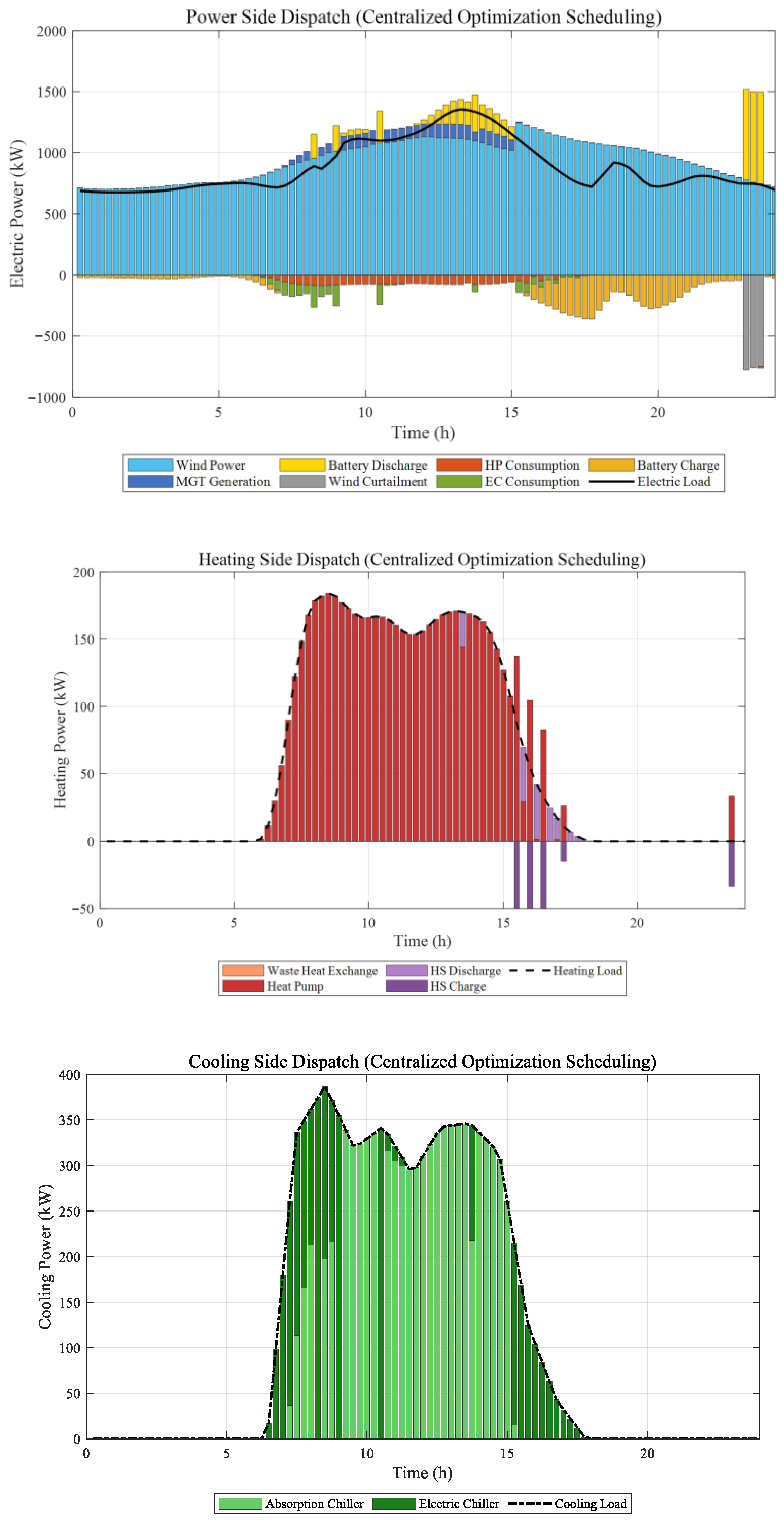
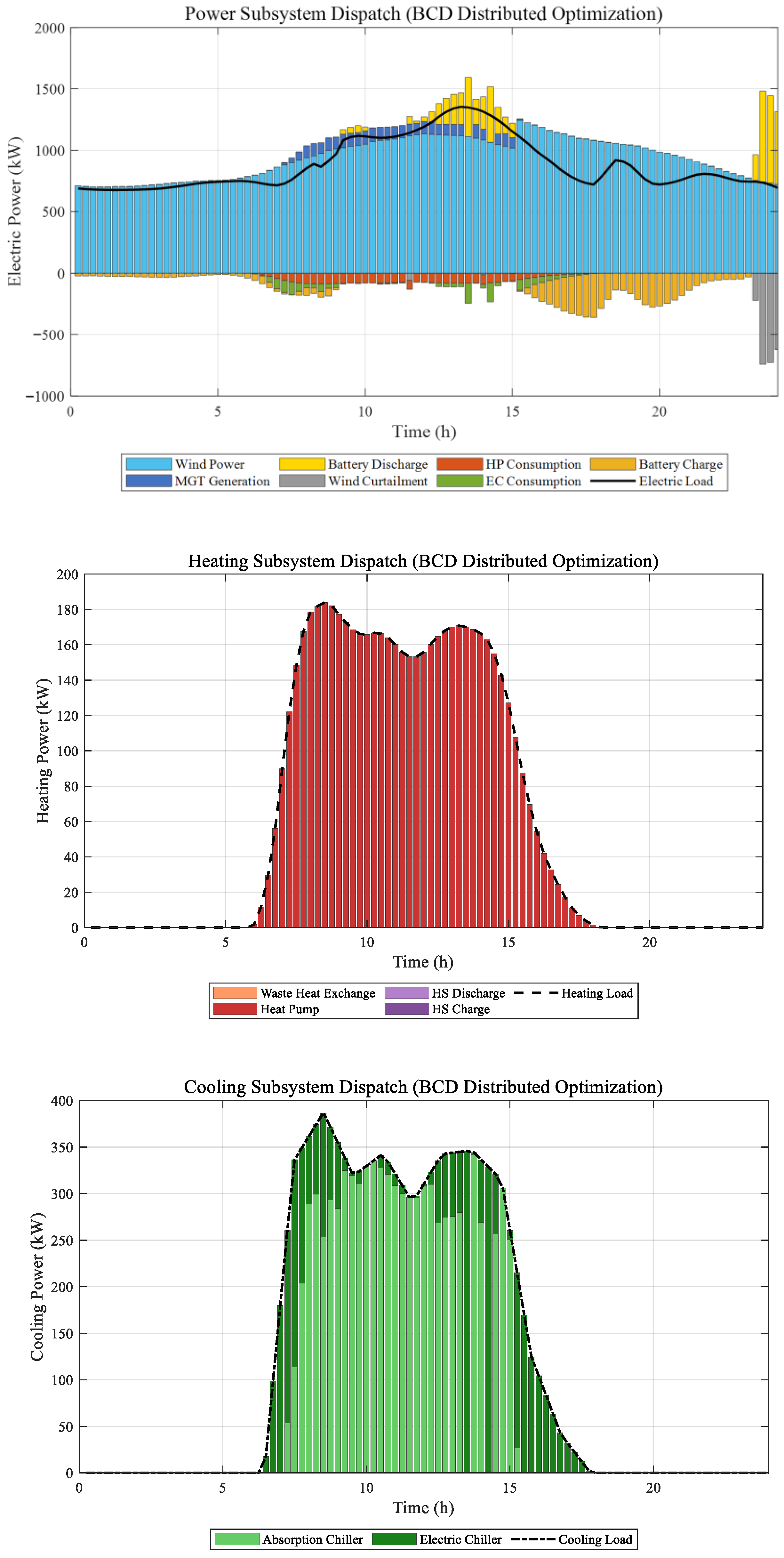
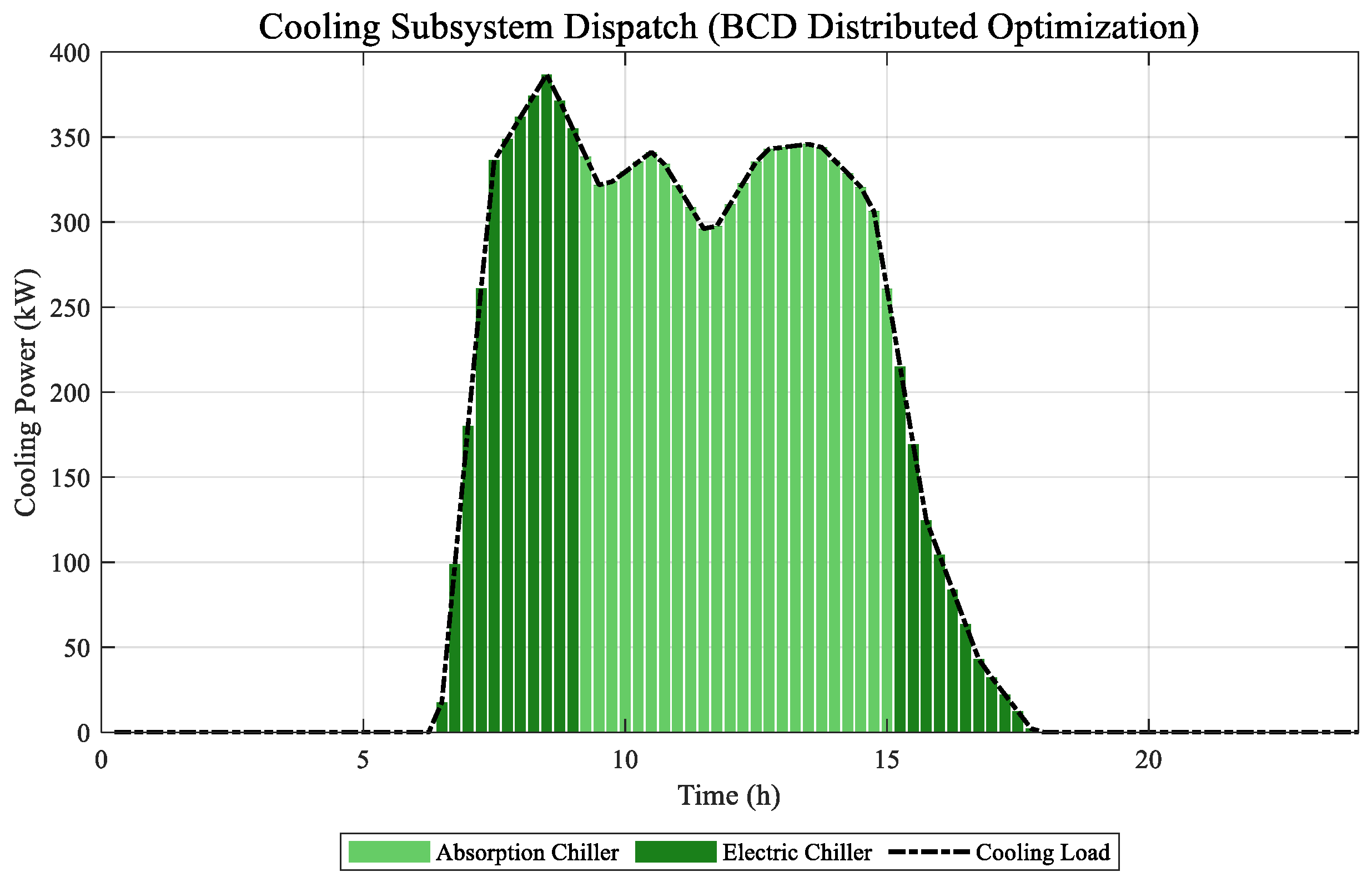
Figure 12, Figure 13, Figure 14, Figure 15 and Figure 16 illustrate the operating states of the main devices and their relationship with the corresponding loads under three scheduling strategies. In these cases, the electricity, heating, and cooling demands, together with the wind power input, are treated as known data, and the dispatch outputs of the energy supply units are obtained through optimization. It should be noted that the distributed stochastic scheduling case considers the uncertainties of both wind power and electric load, and five representative scenarios are constructed using a scenario-based approach. In these cases, the cooling demand is higher than the heating demand, and the lithium bromide chiller has a higher waste heat utilization efficiency than the waste heat exchanger. Therefore, the waste flue gas is preferentially allocated to the cooling side, and the waste heat exchanger is not used. In winter, when the heating demand is much greater than the cooling demand, the waste heat exchanger would be operated.
A comparison between Figure 12 and Figure 13 shows that the centralized deterministic and distributed deterministic schemes yield highly similar results for the electricity and cooling subsystems. The output trajectories and on/off states of major devices, such as the gas turbine and electric chiller, remain largely consistent in both cases, and both strategies can effectively follow the load demand while maintaining wind power utilization. The main differences lie in the scheduling strategies of the thermal energy subsystem: centralized scheduling pursues global economic optimization, resulting in relatively large fluctuations in the output of heat pumps and heat storage equipment, and more frequent switching of charging and discharging states; while in distributed scheduling, the BCD algorithm is used to decouple and alternately iterate among the subsystems, and the transmission of coupling variables to a certain extent plays a smoothing role, making the operation curves of thermal equipment relatively more stable. Although there are minor differences in the response characteristics of local thermal equipment between the two, they can both reliably meet the multi-energy load demands of the integrated energy system as a whole. Additionally, as shown in Figure 14, the BCD algorithm’s iterative curve rapidly descends below the convergence threshold within approximately 17 iterations, fully demonstrating the efficiency and effectiveness of this distributed coordination mechanism.
Figure 12. The centralized deterministic optimal dispatch results of CCHP.
Energies 19 01763 g012
Figure 13. The distributed deterministic optimization scheduling results of CCHP.
Energies 19 01763 g013
Figure 14. Convergence curve of the CCHP distributed deterministic optimization scheduling BCD algorithm.
Energies 19 01763 g014
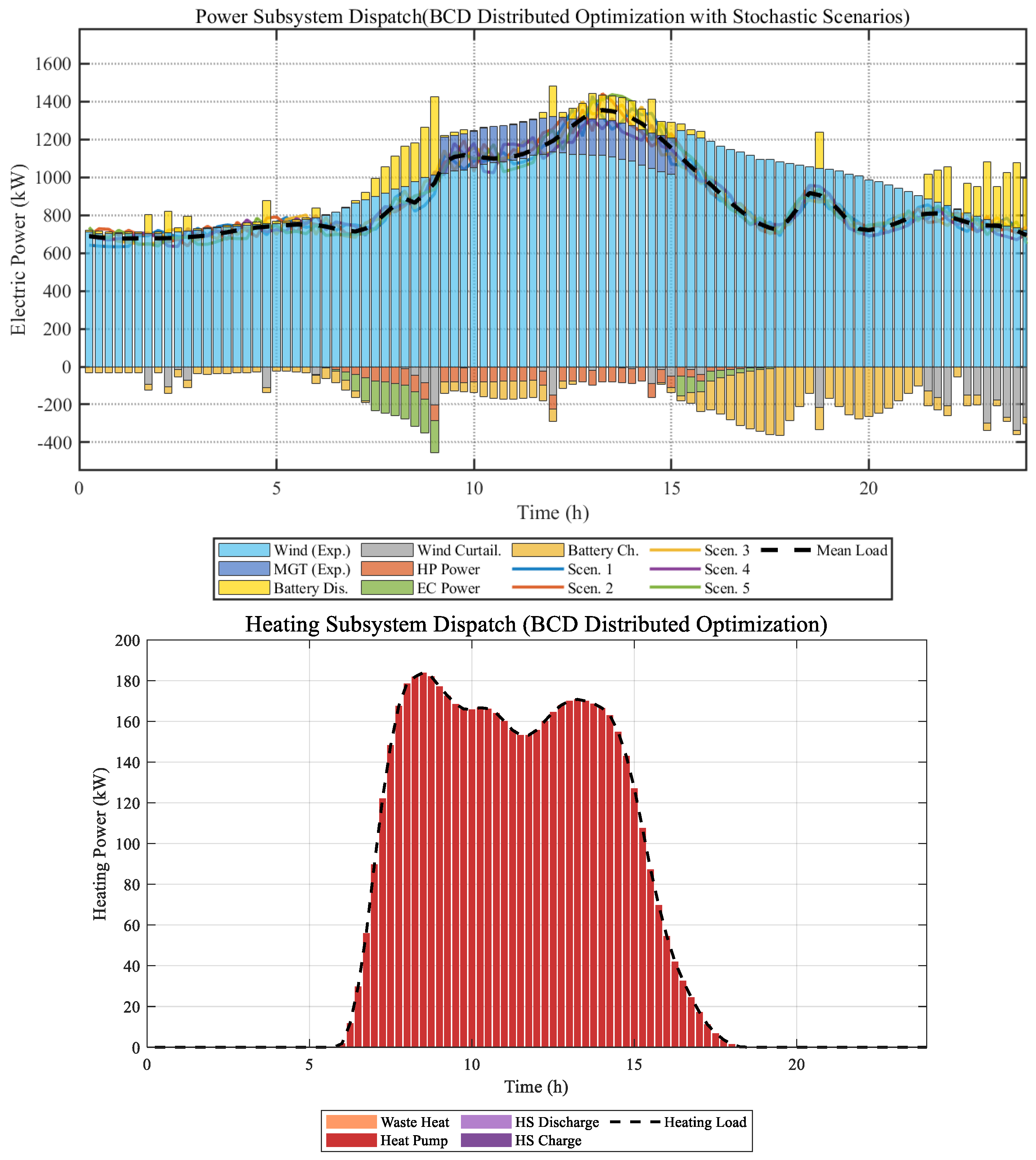
Figure 15. The results of distributed uncertainty optimization scheduling for CCHP.
Energies 19 01763 g015aEnergies 19 01763 g015b
Figure 16. Convergence curve of the CCHP distributed uncertainty optimization scheduling BCD algorithm.
Energies 19 01763 g016
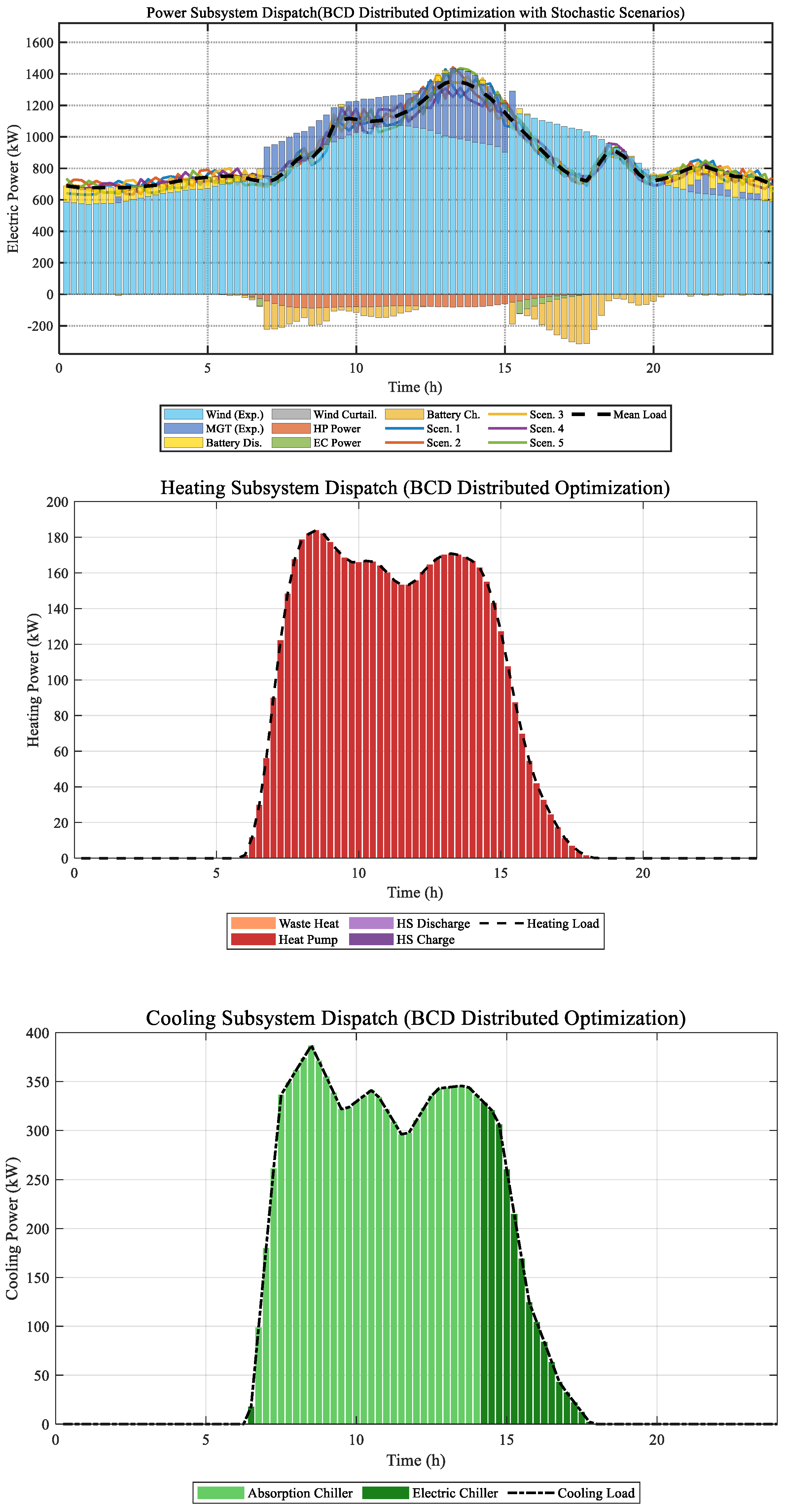
Figure 15 shows the results of distributed stochastic optimization scheduling considering uncertainties. Affected by multiple scenarios of wind power and electricity load, the system adopted a more conservative strategy: the output of gas turbines was generally increased to cope with possible insufficient wind power output; meanwhile, due to excess wind power in some scenarios and the limited system regulation capacity, obvious wind power curtailment occurred. Additionally, the output of electric refrigeration and waste heat utilization equipment also adjusted with the scenarios, and the overall operation curve was more complex than that of deterministic scheduling. The iteration curve in Figure 16 also converged well, indicating that the BCD algorithm can effectively handle distributed optimization problems with chance constraints. In summary, from deterministic to uncertain scheduling, the system paid the price of increased equipment output fluctuations and reduced wind power consumption rate to enhance robustness, but the flexibility of the distributed architecture was still maintained.
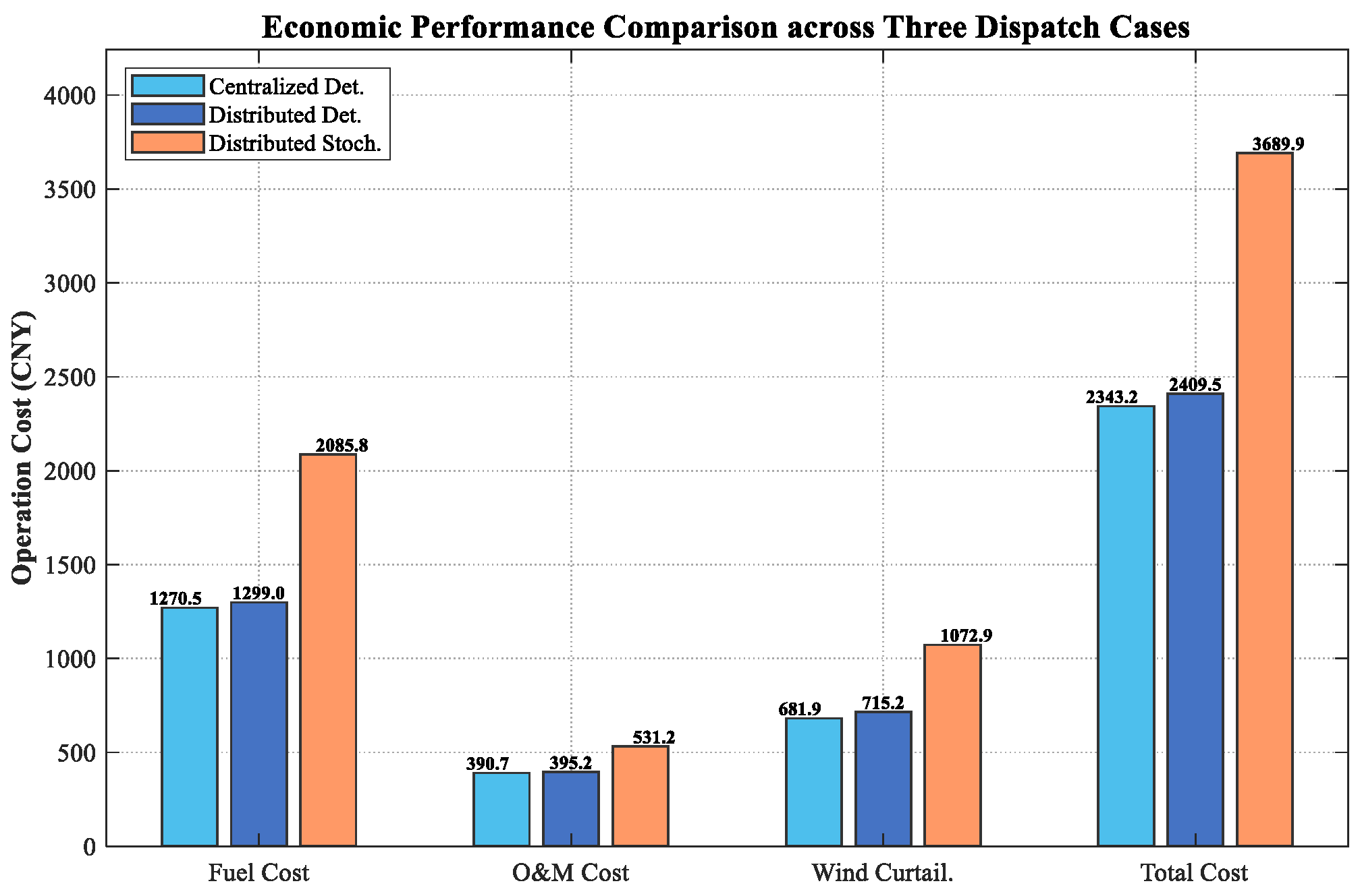
Figure 17 compares the various economic costs of the three scheduling cases, including fuel costs, equipment operation and maintenance costs, and penalty costs for wind curtailment. Overall, the total cost of Case 1 (centralized deterministic) is the lowest (2343.2 ¥), that of Case 2 (distributed deterministic) is slightly higher (2409.5 ¥), and that of Case 3 (distributed stochastic optimization) is the highest (3689.9 ¥).
Case 2 has a slightly higher cost than Case 1, mainly due to the difference in the dispatching architecture. Centralized dispatching has a global perspective and can break through the barriers of subsystems to seek the theoretical optimal solution; distributed dispatching uses the BCD algorithm to coordinate boundaries while preserving the privacy of each entity. This spatial decoupling, while enhancing privacy and autonomy, inevitably leads to a very small loss in global economic efficiency, resulting in a slight increase in fuel costs and wind curtailment costs.
Case 3 has a significantly higher total cost than Cases 1 and 2, with the total cost increasing from 2409.5 ¥ in Case 2 to 3689.9 ¥ in Case 3, i.e., by 53.1%. This increase is mainly caused by the more conservative dispatch strategy adopted under wind-power and electric-load uncertainty. Specifically, to maintain power balance across multiple scenarios, the system relies more on controllable units such as gas turbines, which increases the fuel cost from 1299.0 ¥ to 2085.8 ¥. At the same time, the higher output level and longer operating duration of controllable equipment raise the operation and maintenance cost from 395.2 ¥ to 531.2 ¥. In addition, due to the multi-scenario coordination constraints and limited regulation capability of the system, part of the wind power has to be curtailed in some scenarios, which further increases the wind curtailment penalty from 715.2 ¥ to 1072.9 ¥. Therefore, the 53.1% increase in total cost should be understood as the combined economic effect of additional fuel consumption, increased equipment operation, and higher wind curtailment under uncertainty-aware dispatch.
All optimization problems were solved using Gurobi 12.0.0 on a computer with an Intel Core i7-12800HX CPU, manufactured by Intel Corporation, Santa Clara, CA, USA. The centralized deterministic optimization required about 7.12 s, the distributed deterministic case required about 71 s, and the distributed stochastic optimization converged within 13 iterations and required about 102 s.
In conclusion, although the total cost of distributed stochastic scheduling is the highest, it reflects the transition from idealized deterministic dispatch to uncertainty-aware dispatch under realistic operating conditions. By considering source-side and load-side fluctuations, the proposed scheme can maintain energy balance under uncertainty and reduce the risk of insufficient supply caused by inadequate reserve capacity. Therefore, it provides a more practical basis for the operation of integrated energy systems with high reliability requirements.

5.2.2. Sensitivity Analysis of the Imbalance Tolerance Rate ω

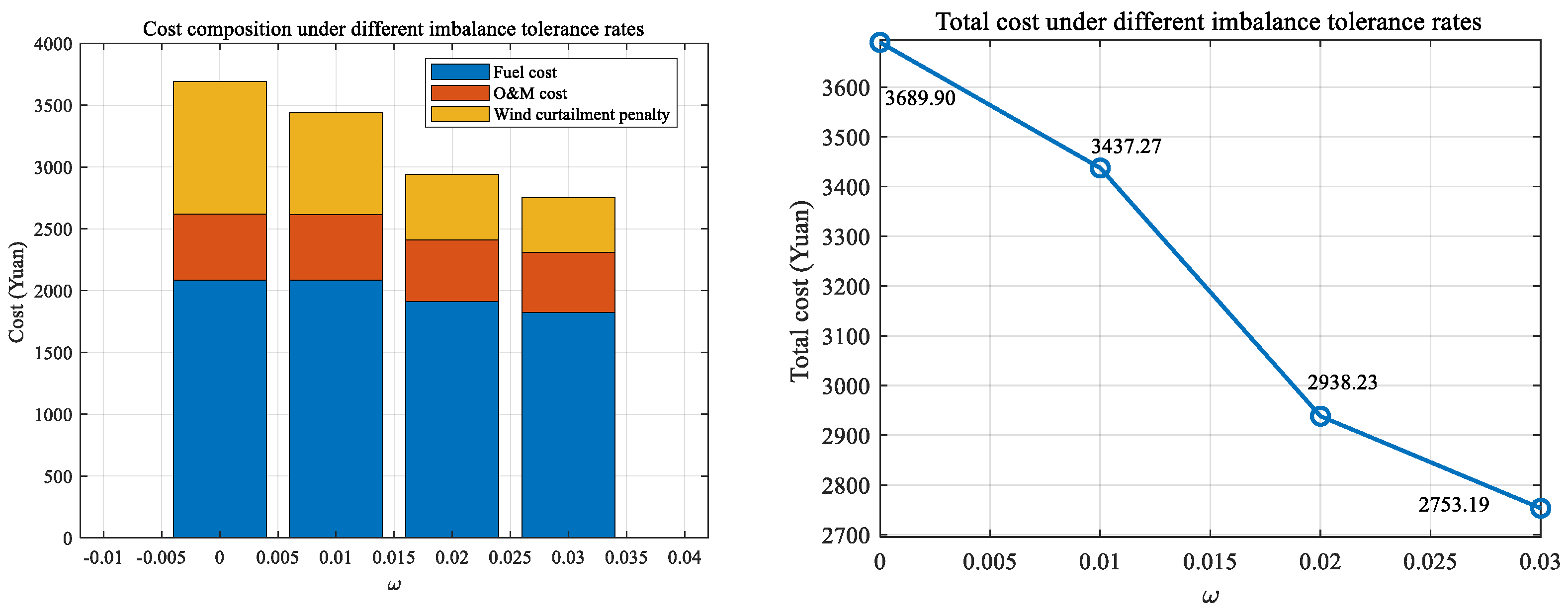
To further analyze the effect of the imbalance tolerance rate ω on stochastic dispatch results, a sensitivity study was conducted under four different ω values, namely ω = 0 ,   0.01 ,   0.02   a n d   0.03 , as shown in Figure 18. The results show that, as ω increases, the total operating cost gradually decreases. This is because a larger ω corresponds to a wider allowable power imbalance interval, which relaxes the power balance constraint under uncertainty and reduces the conservativeness of the dispatch strategy. As a result, the system can operate with greater flexibility, thereby lowering the overall dispatch cost.
In addition, the reduction in total cost mainly comes from the decrease in fuel cost and wind curtailment penalty, while the operation and maintenance cost changes only slightly. This indicates that, as the imbalance tolerance rate increases, the conservativeness of the stochastic dispatch strategy gradually decreases, thereby improving the economic performance of system operation. However, a larger ω also implies that the scheduling model accepts a wider allowable power imbalance interval. Therefore, in practical engineering applications, ω should be determined according to the required tradeoff between economy and operational robustness.

5.3. Analysis of Scheduling Results of Scenario Generation Based on Machine Learning and Traditional Scenario Generation

Based on the stochastic dispatch framework in Case 3, this subsection further compares the economic and operational impacts of two different scenario generation methods, namely the traditional LHS-K means method and the proposed Diffusion-TS method.
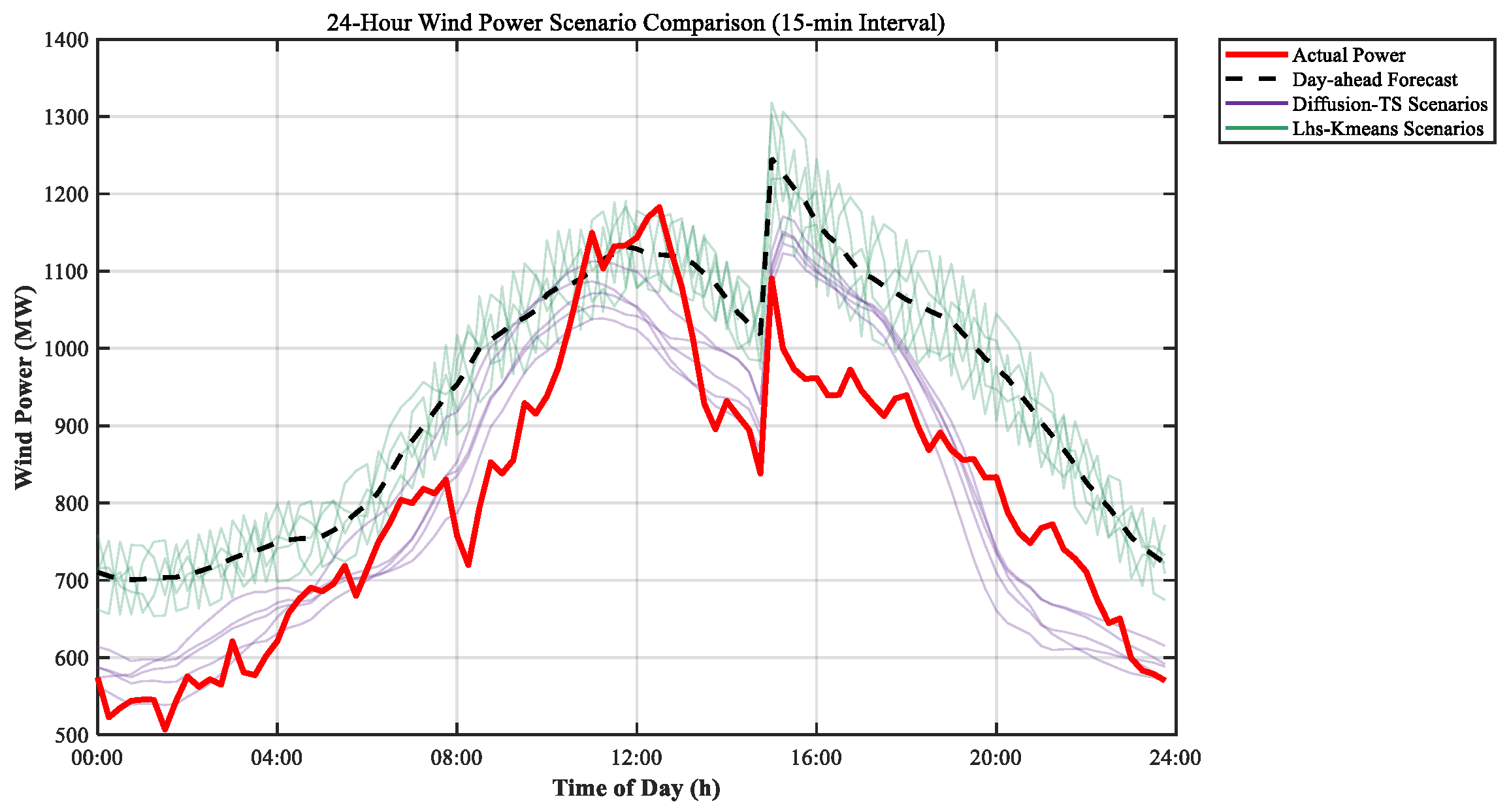
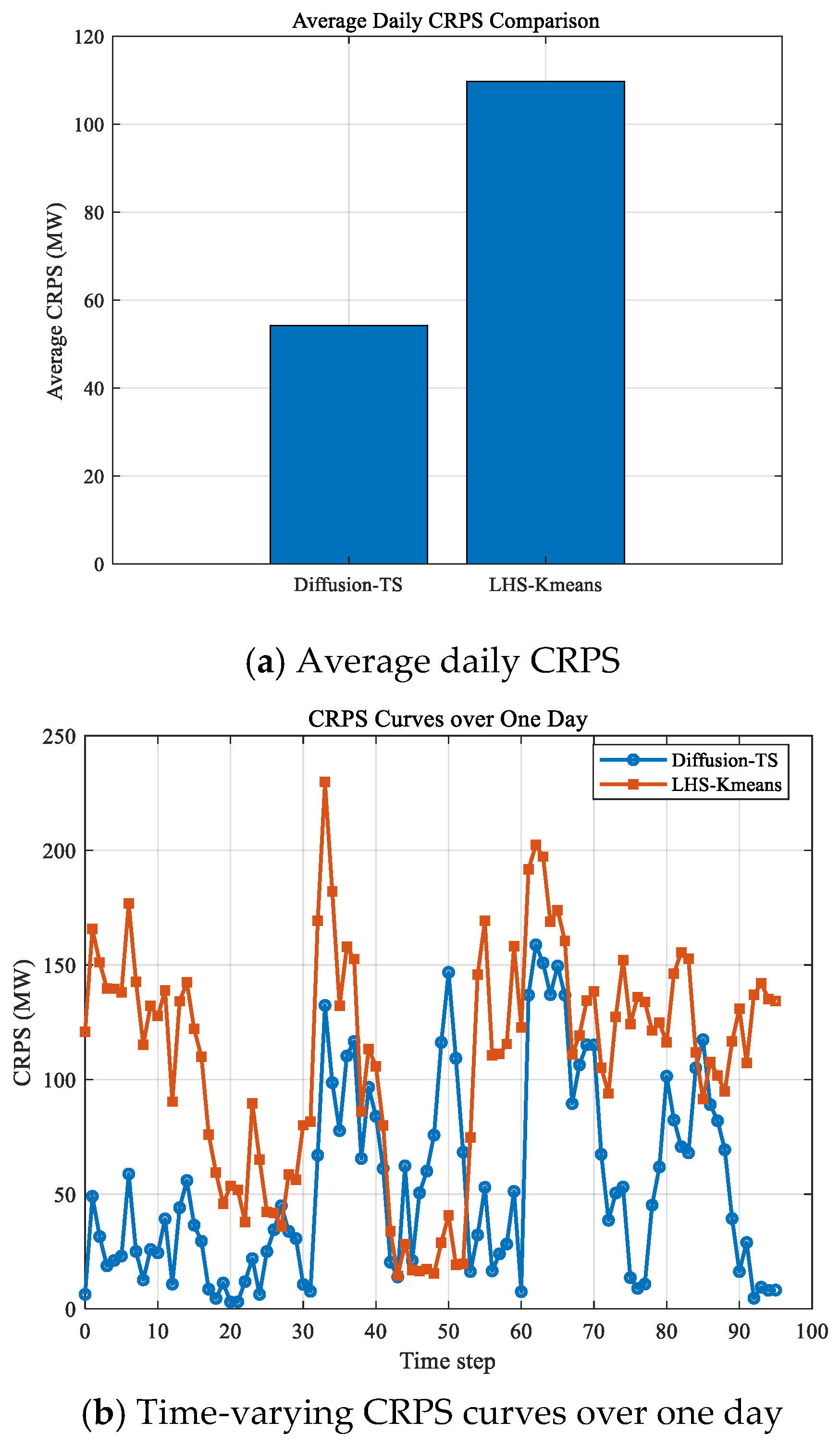
In the distributed uncertainty optimization scheduling of CCHP, the quality of wind power scenarios generation has a decisive impact on the reliability and economy of the scheduling results. Figure 19 shows the comparison of wind power scenarios generated by the two methods. To further quantify the difference in scenario quality, the Continuous Ranked Probability Score (CRPS) is calculated for the generated scenarios on one representative day. As shown in Figure 20a, the average daily CRPS of Diffusion-TS is 54.45 MW, whereas that of LHS-K means is 109.34 MW. Figure 20b further shows that the CRPS values of Diffusion-TS are lower than those of LHS-K means during most dispatch intervals. Because a lower CRPS indicates better agreement between the generated scenario distribution and the actual wind power output, these results quantitatively confirm the superiority of Diffusion-TS in scenario generation.
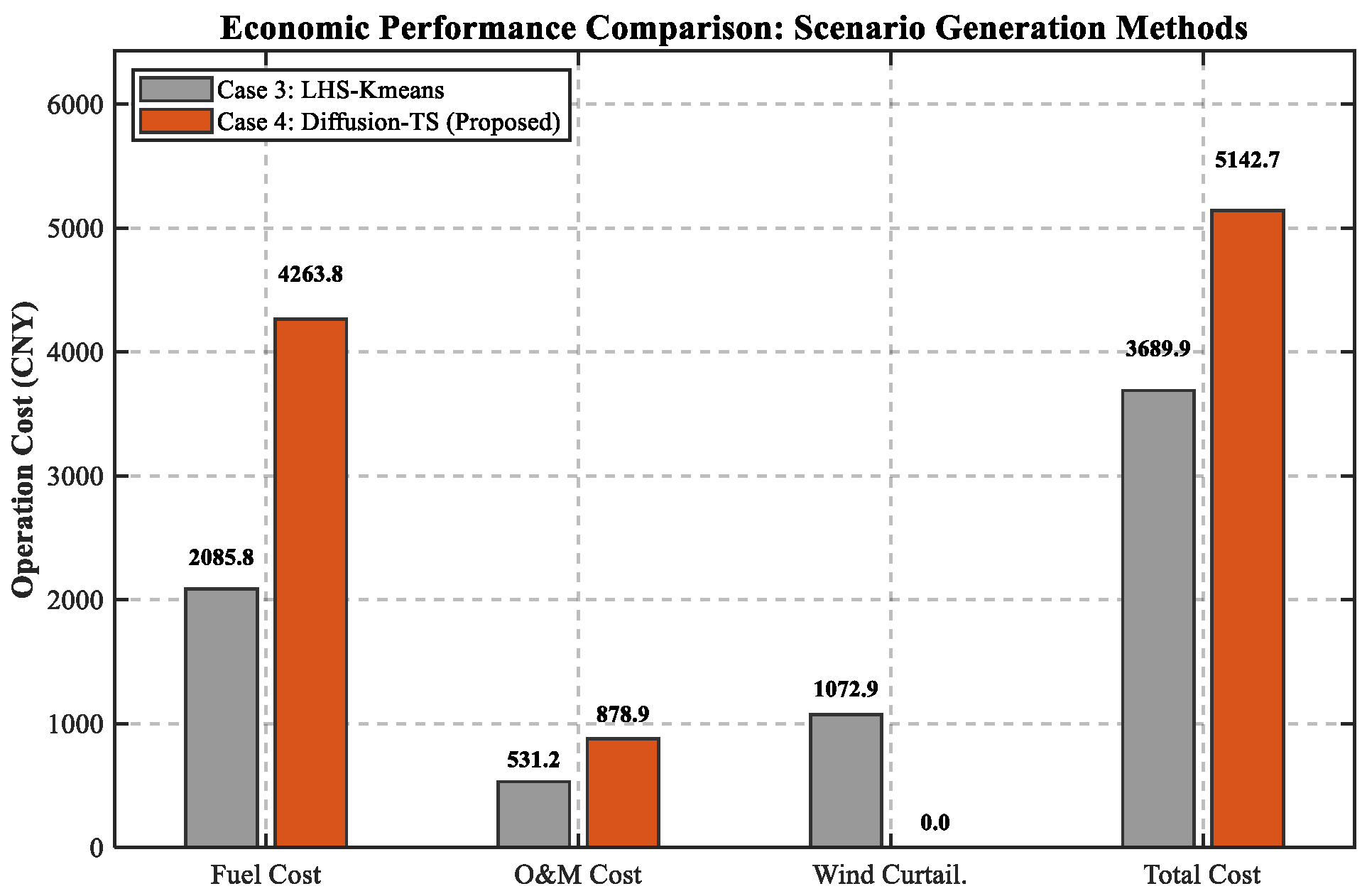
It can also be observed that the scenarios produced by the traditional method are distributed mainly around the day-ahead wind power forecast and generally exhibit a relatively high output level. By contrast, the Diffusion-TS-generated scenarios match the variation pattern and probability distribution of the actual wind power more closely, and they show better temporal smoothness and scenario diversity than those generated by the traditional method. Figure 15 corresponds to the stochastic dispatch result based on the traditional LHS-K means scenarios, whereas Figure 21 shows the stochastic dispatch result based on the Diffusion-TS scenarios. Compared with the traditional scenario generation approach, the wind power scenarios produced by Diffusion-TS are generally more consistent with the actual wind power trajectory and are usually lower than the forecast-centered traditional scenarios. As a result, the available wind power subject to curtailment is reduced, and the wind curtailment loss decreases accordingly. However, since the system receives less wind power support under the Diffusion-TS scenarios, the output of controllable units such as gas turbines must increase to satisfy the load demand, which leads to higher fuel cost and operation and maintenance cost.
Figure 19. Comparison of Diffusion-TS model and LHS-K means in scenario generation.
Energies 19 01763 g019
Figure 20. Quantitative CRPS comparison between Diffusion-TS and LHS-K means.
Energies 19 01763 g020
Figure 21. Distributed uncertainty optimization scheduling results (using Diffusion-TS to generate wind power scenarios).
Energies 19 01763 g021
Figure 22. Convergence curve of BCD algorithm for distributed uncertainty optimization scheduling of CCHP.
Energies 19 01763 g022
Figure 23 further compares the cost under the two stochastic dispatch schemes. Although the dispatch scheme based on Diffusion-TS scenarios leads to a higher total cost, it provides a scenario set that is more consistent with the actual wind power characteristics and therefore yields a more robust dispatch result. This result indicates that improving scenario fidelity may increase the operating cost, but it can provide a more reliable basis for stochastic scheduling under renewable uncertainty.

6. Conclusions

This paper investigates the optimal dispatch of integrated energy systems under source-load uncertainty from two perspectives: high-fidelity wind power scenario generation and distributed stochastic optimal dispatch. The main conclusions are summarized as follows:
(1)
A conditional Diffusion-TS-based wind power scenario generation method driven by day-ahead forecasts is proposed. By incorporating the day-ahead forecast as conditional information into the denoising network, the model learns the relationship between forecasted and actual wind power output and generates high-fidelity wind power scenarios. The test results show that the average CRPS of the generated scenarios is 162.16 MW, which is significantly lower than that of the deterministic forecast benchmark (MAE = 246.00 MW), indicating that the proposed method provides more accurate probabilistic characterization of wind power uncertainty.
(2)
A temperature-based strategy is introduced to balance scenario diversity and fidelity. By dynamically scaling the variance of Gaussian noise during the reverse sampling stage, the uncertainty range of the generated scenarios can be explicitly controlled. Sensitivity analysis shows that the model achieves the best performance at τ = 2, where moderate noise injection enables the generated scenarios to better match the probability distribution of actual wind power output.
(3)
A distributed stochastic optimization scheduling model based on chance constraints is developed. Under the distributed scheduling framework, the power balance constraint is reformulated as a probabilistic constraint and then converted into a tractable mixed-integer linear programming problem through scenario sampling. The proposed method can effectively address the dual uncertainties of wind power and electric load while preserving subsystem privacy and improving power supply reliability under adverse operating conditions.
(4)
A distributed solution framework based on the BCD algorithm is developed, and the impacts of different scenario generation methods on scheduling performance are compared. The case study results show that the BCD algorithm converges within 13 iterations, demonstrating the effectiveness of the distributed coordination mechanism. The total cost of distributed deterministic scheduling is 2.8% higher than that of centralized scheduling, reflecting the economic impact of distributed coordination. The total cost of distributed stochastic scheduling is 53.1% higher than that of distributed deterministic scheduling, mainly due to the increase in fuel cost and wind power curtailment penalty under uncertainty-aware dispatch. Compared with the traditional LHS-K means method, the Diffusion-TS-based scheduling scheme results in a higher total cost, but the generated wind power scenarios are closer to the actual output level, and the resulting dispatch decisions are more consistent with realistic wind power conditions.
In conclusion, the proposed method improves both the quality of wind power scenario generation and the effectiveness of distributed stochastic scheduling, and provides a useful technical framework for the safe and economic operation of integrated energy systems under uncertainty. Future work may further consider coupled uncertainties of multi-energy loads, the integration of demand response mechanisms, and the development of more efficient distributed solution algorithms. Moreover, since the present study mainly focuses on high-fidelity scenario generation and its application in stochastic scheduling, more comprehensive sensitivity analysis and quantitative reliability evaluation will be further carried out in future work to investigate the economic–reliability tradeoff of the dispatch framework.

Author Contributions

Conceptualization, L.S. and L.P.; methodology, L.S., L.P. and P.X.; software, P.X.; validation, P.X.; formal analysis, P.X.; investigation, C.C.; data curation, C.C. and P.X.; writing—original draft preparation, C.C. and P.X.; writing—review and editing, L.S. and L.P.; supervision, L.P. All authors have read and agreed to the published version of the manuscript.

Funding

This research received no external funding.

Data Availability Statement

The original contributions presented in this study are included in the article. Further inquiries can be directed to the corresponding author.

Conflicts of Interest

The authors declare no conflicts of interest.

References

  1. Song, D.; Meng, W.; Dong, M.; Yang, J.; Wang, J.; Chen, X.; Huang, L. A critical survey of integrated energy system: Summaries, methodologies and analysis. Energy Convers. Manag. 2022, 266, 115863. [Google Scholar] [CrossRef] [Scilit]
  2. Song, C.; Yuan, Y.; Dai, L. Distributionally robust optimization of virtual power plant bidding strategies considering discrete scenario-based uncertainties in day-ahead market prices and wind powers. Electr. Power Syst. Res. 2025, 248, 111977. [Google Scholar] [CrossRef] [Scilit]
  3. Wu, Q.; Li, C. Modeling and operation optimization of hydrogen-based integrated energy system with refined power-to-gas and carbon-capture-storage technologies under carbon trading. Energy 2023, 270, 126832. [Google Scholar] [CrossRef] [Scilit]
  4. Zhu, F.; Zhao, L.; Liu, W.; Zhu, O.; Hou, T.; Li, J.; Guo, X.; Zhong, P. A stochastic optimization framework for short-term peak shaving in hydro-wind-solar hybrid renewable energy systems under source-load dual uncertainties. Appl. Energy 2025, 400, 126597. [Google Scholar] [CrossRef] [Scilit]
  5. Li, F.; Wang, D.; Guo, H.; Zhang, J. Distributionally Robust Optimization for integrated energy system accounting for refinement utilization of hydrogen and ladder-type carbon trading mechanism. Appl. Energy 2024, 367, 123391. [Google Scholar] [CrossRef] [Scilit]
  6. Han, X.; Lv, F.; Li, J.; Zeng, F. Flexible interactive control method for multi-scenario sharing of hybrid pumped storage-wind-photovoltaic power generation. J. Energy Storage 2024, 100, 113590. [Google Scholar] [CrossRef] [Scilit]
  7. Munkhammar, J. Very short-term probabilistic and scenario-based forecasting of solar irradiance using Markov-chain mixture distribution modeling. Sol. Energy Adv. 2024, 4, 100057. [Google Scholar] [CrossRef] [Scilit]
  8. Wang, J.; Zhang, X.; Wang, Y.; Yang, S.; Wang, S.; Xie, Y.; Gong, J.; Lin, J. Power system source-load forecasting based on scene generation in extreme weather. Energy 2025, 330, 136991. [Google Scholar] [CrossRef] [Scilit]
  9. Liu, X.; Yu, J.; Gong, L.; Liu, M.; Xiang, X. A GCN-based adaptive generative adversarial network model for short-term wind speed scenario prediction. Energy 2024, 294, 130931. [Google Scholar] [CrossRef] [Scilit]
  10. Li, Z.; Peng, X.; Cui, W.; Xu, Y.; Liu, J.; Yuan, H.; Lai, C.; Lai, L. A novel scenario generation method of renewable energy using improved VAEGAN with controllable interpretable features. Appl. Energy 2024, 363, 122905. [Google Scholar] [CrossRef] [Scilit]
  11. Arjovsky, M.; Bottou, L. Towards Principled Methods for Training Generative Adversarial Networks. In Proceedings of the International Conference on Learning Representations (ICLR), Toulon, France, 24–26 April 2017. [Google Scholar]
  12. Xu, Y.; Zhang, J.; Lu, D.; Li, S.-T.; Li, Q.; Yu, X. An image expansion method based on Wasserstein generative adversarial network for surface defects of fair-faced concrete. Eng. Appl. Artif. Intell. 2026, 171, 114219. [Google Scholar] [CrossRef] [Scilit]
  13. Min, W.; Wu, W.; Zhang, G.; Zheng, L. FuncScene: Function-centric indoor scene synthesis via a variational autoencoder framework. Comput. Aided Geom. Des. 2024, 111, 102319. [Google Scholar] [CrossRef] [Scilit]
  14. Ho, J.; Jain, A.; Abbeel, P. Denoising Diffusion Probabilistic Models. Adv. Neural Inf. Process. Syst. 2020, 33, 6840–6851. [Google Scholar]
  15. Rombach, R.; Blattmann, A.; Lorenz, D.; Esser, P.; Ommer, B. High-Resolution Image Synthesis with Latent Diffusion Models. In Proceedings of the IEEE/CVF Conference on Computer Vision and Pattern Recognition (CVPR), New Orleans, LA, USA, 18–24 June 2022; pp. 10684–10695. [Google Scholar]
  16. Yang, L.; Zhang, Z.; Song, Y.; Hong, S.; Xu, R.; Zhao, Y.; Zhang, W.; Cui, B.; Yang, M. Diffusion Models: A Comprehensive Survey of Methods and Applications. ACM Comput. Surv. 2024, 56, 1–39. [Google Scholar]
  17. Vetter, J.; Macke, J.; Gao, R. Generating realistic neurophysiological time series with denoising diffusion probabilistic models. Patterns 2024, 5, 101047. [Google Scholar] [CrossRef] [Scilit]
  18. Lim, H.; Kim, M.; Park, S.; Park, N. Regular Time-series Generation using SGM. arXiv 2023, arXiv:2301.08518. [Google Scholar] [CrossRef] [Scilit]
  19. Liu, S.; Li, X.; Cong, G.; Chen, Y.; Jiang, Y. Multivariate time-series imputation with disentangled temporal representations. In Proceedings of the Eleventh International Conference on Learning Representations (ICLR), Kigali, Rwanda, 1–5 May 2022. [Google Scholar]
  20. Yuan, X.; Qiao, Y. Diffusion-TS: Interpretable Diffusion for General Time Series Generation. In Proceedings of the International Conference on Learning Representations (ICLR), Vienna, Austria, 7–11 May 2024. [Google Scholar]
  21. Lu, S.; Wu, D.; Ma, Y. Graph-EXTRA enabled distributed optimal dispatch for integrated energy system in steel industry under uncertainties. Case Stud. Therm. Eng. 2026, 78, 107684. [Google Scholar] [CrossRef] [Scilit]
  22. Chong, Z.; Yang, L.; Gao, Y.; Song, X. Optimal dispatch strategy for electricity-heat integrated energy system considering multiple flexibility-enhancing methods. Energy Convers. Manag. 2025, 337, 119901. [Google Scholar] [CrossRef] [Scilit]
  23. Chen, R.; Liao, L.; Song, D.; Wei, C.; Yang, J.; Talaat, M.; Elkholy, M. Two-stage optimization scheduling strategy for virtual power plants considering the correlated uncertainty of distributed energy storage in extreme scenarios. Appl. Energy 2026, 409, 127477. [Google Scholar] [CrossRef] [Scilit]
  24. Telle, J.-S.; Schönfeldt, P.; Schlüters, S.; Hanke, B.; von Maydell, K. Stochastic net load optimization in distributed integrated energy systems—A forecast based scheduling approach. Smart Energy 2026, 21, 100228. [Google Scholar] [CrossRef] [Scilit]
  25. Wu, S.; Wang, Y.; Liu, L.; Yang, Z.; Cao, Q.; He, H.; Cao, Y. Two-stage distributionally robust optimal operation of rural virtual power plants considering multi correlated uncertainties. Int. J. Electr. Power Energy Syst. 2024, 161, 110173. [Google Scholar] [CrossRef] [Scilit]
  26. Gu, W.; Wang, J.; Lu, S.; Luo, Z.; Wu, C. Optimal operation for integrated energy system considering thermal inertia of district heating network and buildings. Appl. Energy 2017, 199, 234–246. [Google Scholar] [CrossRef] [Scilit]
  27. Wang, R.; Wen, X.; Wang, X.; Fu, Y.; Zhang, Y. Low carbon optimal operation of integrated energy system based on carbon capture technology, LCA carbon emissions and ladder-type carbon trading. Appl. Energy 2022, 311, 118664. [Google Scholar] [CrossRef] [Scilit]
  28. Chen, X.; Wu, X. The roles of carbon capture, utilization and storage in the transition to a low-carbon energy system using a stochastic optimal scheduling approach. J. Clean. Prod. 2022, 366, 132860. [Google Scholar] [CrossRef] [Scilit]
  29. Chang, D.; Shen, J.; Zhang, J. Day-ahead and Intraday Optimal Dispatch Schedule for MGT-IES Considering the Dynamic Characteristics of Main Equipment. In Proceedings of the IEEE International Conference on Power Renewable Energy (ICPRE), Shanghai, China, 24–26 September 2021. [Google Scholar]
Figure 1. Schematic illustration of the combined cooling, heating and power system.
Energies 19 01763 g001
Figure 2. Framework diagram of wind power scenario generation method based on Diffusion-TS.
Energies 19 01763 g002
Figure 3. The framework diagram of the method proposed in the paper.
Energies 19 01763 g003
Figure 4. Training loss curve of the Diffusion-TS model.
Energies 19 01763 g004
Figure 5. Sensitivity analysis diagram of temperature parameter τ.
Energies 19 01763 g005
Figure 6. The error variation curves of the day-ahead forecast (MAE) and the Diffusion-TS scenario generation (CRPS).
Energies 19 01763 g006
Figure 7. The relationship between the scatter distribution of the day-ahead forecast (MAE) and the Diffusion-TS scenario generation (CRPS).
Energies 19 01763 g007
Figure 8. The error variation curves of the nowcasting (nMAE) and scenario generation (nCRPS).
Energies 19 01763 g008
Figure 9. Comparison of probability density distributions of prediction errors from different methods.
Energies 19 01763 g009
Figure 10. Trend chart of wind power and changes in electricity, heating and cooling loads.
Energies 19 01763 g010
Figure 11. Electric load and wind power output scenario generation curves.
Energies 19 01763 g011
Figure 17. Comparison of economic costs of CCHP systems under three scheduling strategies.
Energies 19 01763 g017
Figure 18. Cost analysis under different imbalance tolerance rates.
Energies 19 01763 g018
Figure 23. Comparison of uncertainty scheduling results between traditional scenario generation and Diffusion-TS scenario generation.
Energies 19 01763 g023
Table 1. Capacity of each device in the CCHP system.
EquipmentCapacityEquipmentCapacity
Storage battery6312 kWhGas turbine800 kW
Heat storage tank100 kWhLithium bromide chiller1871 kW
Waste heat exchanger725 kWHeat pump1224 kW
Electric chiller650 kW
Disclaimer/Publisher’s Note: The statements, opinions and data contained in all publications are solely those of the individual author(s) and contributor(s) and not of MDPI and/or the editor(s). MDPI and/or the editor(s) disclaim responsibility for any injury to people or property resulting from any ideas, methods, instructions or products referred to in the content.