Article

Dynamic Robust Generation and Transmission Expansion Planning Incorporating Novel Inter-Area Virtual Transmission Lines and Unit Commitment Ramping Constraints †

by
Flavio Arthur Leal Ferreira
* and
Clodomiro Unsihuay Vila
Department of Electrical Engineering, PPGEE, UFPR—Universidade Federal do Paraná, Curitiba 81530-900, Brazil
*
Author to whom correspondence should be addressed.
This paper is an extended version of our paper published in Energies2025, 18, 1602.
Energies 2026, 19(7), 1759; https://doi.org/10.3390/en19071759
Submission received: 1 March 2026 / Revised: 26 March 2026 / Accepted: 31 March 2026 / Published: 3 April 2026

Abstract

Generation and transmission expansion planning (GTEP) faces increasing challenges from variable renewable energy integration, inter-area transmission congestion, and the need for cost-effective flexibility. This study extends a prior data-driven distributionally robust optimization framework by introducing inter-area virtual transmission lines (VTL), enabled through strategic energy storage system (ESS) allocation within network areas, to optimize and potentially defer investments in trunk transmission lines, while adding a unit commitment (UC) level considering ramping constraints to address short-term net demand variability. The model incorporates flexibility from transmission and distribution system operators interconnection (TSO-DSO), quantified via a selected state-of-the-art metric integrated into ramping and flexibility constraints, with required levels derived from associated DSO planning. A linear AC optimal power flow is employed, and uncertainties in demand and variable renewable generation are handled using data-driven distributionally robust optimization within a three-level architecture: column-and-constraint generation with duality-free decomposition at the core, augmented by unit commitment. Case studies on the IEEE RTS-GMLC network demonstrate significant reductions in total system costs (operations, investments, and flexibility provisions), improved transmission efficiency, and enhanced flexibility metrics, confirming the value of localized ESS deployment and high-resolution ramping in modern low-carbon power systems.

1. Introduction

1.1. Background

In recent years, the increasing integration of renewable energy sources, evolving market structures, and heightened concerns over environmental impacts have significantly transformed the landscape of power system planning. The challenge of expanding generation and transmission infrastructure to accommodate these changes while maintaining reliability, efficiency, and economic viability has become more complex and urgent. Building on the foundational work presented in our previous publication [1], which proposed a comprehensive long-term expansion model accounting for storage and renewable integration, this article seeks to address the challenges related to operational flexibility and short-term variability, thereby enhancing the robustness of the planning framework for modern power systems.
Grid boosters, also known as virtual transmission lines (VTLs), use large-scale battery energy storage systems (BESSs) placed strategically in the grid to increase the capacity and stability of existing power lines, especially for integrating renewables. As an alternative to capital-intensive physical infrastructure expansion, these batteries quickly inject or absorb power (real and reactive) to manage congestion, allowing lines to run near full capacity safely, thereby increasing renewable energy transport from areas like northern Germany to industrial centers [2,3,4].
This work advances the original expansion planning model by incorporating an additional level of analysis to capture the system’s short-term operational constraints to ensure system flexibility and feasibility. Building upon the initial framework, which focused on long-term generation and transmission expansion considering a new “Booster and Stacker Inter-Area Virtual Transmission (BSIAVT)” concept, battery energy storage and variable renewable energy integration, the new model introduces a third, higher-resolution layer that explicitly accounts for unit commitment (UC) and generator ramping constraints. This new level addresses the short-term variability of intermittent renewable resources and the operational flexibility required for reliable system management.
The proposed BSIAVT concept is an innovative method in power systems that uses large-scale BESSs to increase the effective and profitable power transfer capacity of existing inter-area transmission lines. The term “Stacker” refers to revenue stacking, where the BESS provides multiple services, such as the above congestion relief, frequency response, and ancillary services, to maximize its economic return and contribution to grid flexibility. The term “Booster” refers to increasing transmission capacity because it reduces bottlenecks, thereby decreasing the need for high-cost redispatch and the curtailment of low-cost, renewable energy. Projects based on the “Grid Booster” concept are currently being implemented by TSOs in Germany and are a form of storage-as-transmission asset (SATA).
Both BSIAVT and the system’s short-term operational constraints via unit commitment are critically important across both the operation (short-term) and expansion planning (long-term) horizons of modern power systems, particularly those integrating high levels of renewable energy. Their importance stems from their ability to manage system flexibility, mitigate the risk of grid congestion, and optimize overall system costs.
The short-term operational model is integrated with the original planning framework through a soft-link methodology, enabling a cohesive decision-making process that considers both long-term investment strategies and short-term operational realities. By enhancing the model’s temporal resolution and operational detail, this evolution aims to provide more accurate insights into the system’s behavior under high renewable penetration and variability, supporting more robust and efficient expansion planning in modern power systems.
This study proposes a dynamic, multi-period robust GTEP model that co-optimizes generation, transmission, and strategic ESS-based inter-area virtual transmission lines over an extended planning horizon, while embedding detailed unit commitment and ramping constraints to ensure operational feasibility across investment periods. Unlike prior works focused on static/target-year planning, GEP-only models, or TEP with simplified one period UC checks, our framework captures sequential investment dynamics under uncertainty.

1.2. Literature Review

The expansion planning of generation and transmission infrastructure constitutes a complex, long-term optimization challenge that typically requires a multi-stage analysis across an extended planning horizon to account for evolving demand, technology costs, and policy constraints. Comprehensive overviews of the field and key methodological developments can be found in the literature, including the surveys by [5,6,7].
In the context of electrical power systems, long-term expansion planning for generation and transmission infrastructure plays a pivotal role in ensuring operational reliability and efficiency. This planning horizon, often spanning years or decades, anticipates future demand growth, technological advancements, and policy shifts, such as the integration of variable renewable energy (VRE) sources like wind and solar. By strategically expanding generation capacity and transmission networks, long-term planning can provide the resources, such as diverse generators, storage capacities, and grid interconnections, that enable daily operations to commit sufficient units effectively. Without adequate long-term provisions, short-term unit commitment processes could face resource shortages, leading to increased costs, reliability risks, or curtailed renewables, as highlighted in studies on generation expansion planning (GEP) models that incorporate UC constraints for realistic feasibility assessments [8,9,10].
The design of long-term GTEP models can be significantly enhanced by recognizing that the value of new infrastructure lies partly in the planned flexibility resources it provides for real-time grid management. As demonstrated by [11], the available capacity of transmission lines is a critical factor enabling short-term operational switching, allowing the grid to be dynamically reconfigured in response to renewable energy volatility and contingency events. Their framework highlights that optimal transmission switching (OTS) serves as a primary tool for leveraging grid-side flexibility; however, the effectiveness of these corrective actions is inherently limited by the physical topology and transmission line capacity decisions established through long-term GTEP models.
The article [12] highlights that traditional energy-based UC formulations used in GEP intrinsically overestimate flexibility and may lead to infeasible ramping constraints. It proposes a novel power-based UC model which precisely models flexibility capabilities and real-time flexibility requirements, including detailed ramping constraints, operating reserves, minimum up/down times, and network constraints.
The research [13] presents a generation expansion model that addresses the conflict between the temporal variability of variable renewables and limited system flexibility at the planning stage. The model determines investment decisions and full-year, hourly power balances in a single optimization framework. The formulation incorporates flexibility constraints, including ramping, and reserve.
The efficiency of electric power systems needs to be intrinsically tied to long-term energy system transmission expansion and generation expansion planning models, which are crucial for analyzing the system transition roadmap and optimizing investments in resources like flexible generators, intermittent renewable energy sources, transmission capacity, and storage resources. Traditionally, generation and transmission expansion planning (GTEP) models often neglected detailed operational constraints typically reserved for UC models due to computational limitations. However, it is critical that the long-term planned expansion provides the necessary flexible resources because neglecting operational constraints in planning models risks generating infeasible or suboptimal investment solutions, leading to outcomes such as reserve shortages and load, or generation shedding, in daily operation. Consequently, incorporating operational flexibility details ensures that daily UC has sufficient available resources to commit [14,15].
The UC problem, central to power system operations, has been fundamentally challenged by the large-scale integration of VRE, demanding advancements in modeling operational flexibility, particularly regarding generator ramping capabilities and volatile net demand.
The presence of intermittent and uncertain VRE requires power systems to become more flexible to accommodate the resulting variability and uncertainty in power outputs. This continuous uncertainty, originating from both renewable energy and demands, has driven the development of stochastic unit commitment (SUC) models, which are viewed as promising tools. SUC typically utilizes advanced techniques like two-stage stochastic programming or robust optimization to handle predictable uncertainties, allowing for better integration of renewable energy and non-generation resources.
The research [16] examines the importance of incorporating operational scenarios representing short-term stochasticity into long-term generation expansion models due to the high shares of VRE.
The increasing variability and unpredictability of VRE intensify the growth of variability and uncertainty in the system net demand (actual demand minus total renewable generation). Deviations from forecasted renewable outputs compel conventional flexible generators and storage resources to ramp up/down quickly to maintain power balance.
Generator ramping constraints (which govern ramp-up and ramp-down limits) are critical technical constraints in UC models. These constraints dictate how fast thermal units can adjust their power output. Ignoring these details in planning models can lead to suboptimal or infeasible investment solutions and an underestimation of operational costs. Ramping constraints must also respect specific limits when a generator is starting up or shutting down.
The research [17] investigates modeling choices, showing that omitting ramps and reserves degrades solutions significantly but reduces computation time; however, linear relaxations yield minor quality loss, especially when minimizing curtailment in VRE intensive scenarios.
GEP and GTEP models can be static or dynamic. Static expansion planning models typically focus on determining the optimal investment mix for a single target year or period of time. In contrast, dynamic or multi-period expansion planning models divide the overall time horizon into multiple periods to evaluate system expansion sequentially. Dynamic models consider several investment horizons in a dynamic manner, allowing for the co-optimization of investments across these various time periods.
The research presented in [18], using a DC power flow model, proposes a static GTEP, considering VRE uncertainties, UC constraints, flexibility, and reserves.
The article [19] proposes a GEP model, using a soft-linking methodology to consider UC constraints to support a short-term hydro-thermal model to schedule generation.
A proposal of a flexibility-oriented robust TEP model that incorporates UC constraints, modeling short-term flexibility requirements, is presented in [20]. The model includes constraints regarding minimum up-time and down-time requirements, minimum production outputs, ramping limits, and start-up/shut-down costs of generator units. It is considered a static expansion planning model that uses a single set of investment decisions.
To explicitly manage this intensified ramping need caused by net demand variability, transmission system operators (TSOs) have been introduced; they can utilize flexible ramping products (FRP) into day-ahead (DA) market models. FRP is distinct from traditional contingency reserves and regulation, serving as reserved ramp capability deployed continuously in real-time (RT) scheduling processes to address expected net demand changes between periods.
The research [21] proposes an enhanced FRP in day-ahead scheduling, designing ramp capabilities adaptive to 15 min net load variability and uncertainty, validated on IEEE test systems to reduce real-time imbalances. This addresses the pitfalls of ignoring intra-hour ramps, where VRE intermittency demands faster response times.
However, traditional FRP design based purely on hourly ramping requirements often fails to accommodate steep intra-hour (e.g., 15 min) net demand changes. This inadequacy, where hourly reserved ramp capabilities cannot meet the rapid dynamics of the subsequent short-term markets (such as the fifteen-minute market (FMM) of CAISO), is a key concern. Consequently, enhanced FRP designs have been proposed that incorporate the impacts of 15 min net load variability and uncertainty into the hourly DA FRP allocation. The goal is to improve efficiency and commit ramp-responsive resources, enhancing system reliability and reducing operating costs in the shorter scheduling granularity markets. The role of energy storage systems (ESSs) is crucial here, as they provide a complementary approach, offering upward ramping flexibility without having to generate long-term energy, thereby mitigating the impacts of intermittent renewable energy outputs and avoiding curtailment during high-VRE-instability periods.
The research [22] proposed a semi-empirical model for lithium-ion battery degradation, distinguishing between calendar and cycle aging effects. The model integrates solid electrolyte interphase (SEI) formation, temperature, state-of-charge (SoC), and depth-of-discharge (DoD) stress factors, using a rainflow cycle-counting algorithm for irregular profiles. This enables lifetime estimation under stochastic operations like frequency regulation and has been applied to evaluate degradation costs in battery energy storage systems for power applications.
ESS use for grid frequency control is considered in [23] with the introduction of a robust control scheme using a hidden Markov jump system (HMJS) with an asynchronous sliding mode observer (ASMO) and observer-based sliding mode control (OSMC) to stabilize inverter-fed power systems during contingencies like line faults. Validation on an IEEE 9-bus system showed effective post-contingency frequency and voltage support in renewable-rich grids.
Expansion capacity of ESS infrastructure is considered in [24]; an optimal ESS sizing method was developed for non-array wind farms, accounting for multi-directional wake (MDW) effects on frequency support. Using an MDW model with characteristic wind directions and fuzzy K-means clustering of wind turbines by frequency support margin (FSM), the approach maximizes FSM coherency via ESS allocation, with case studies demonstrating improved performance.
Table 1 and Table 2 compare the planning models and solution approaches reviewed in the literature with the methodology proposed in this article, highlighting key characteristics such as temporal resolution, technical detail, flexibility representation, and treatment of short-term variability.
While there are studies that incorporate UC in GEP or TEP, and some address coordinated GTEP with ramping considerations, these typically employ approaches without inter-area virtual transmission concepts like BSIAVT for deferring trunk investments and do not integrate high-resolution UC ramping within a dynamic multi-period GTEP framework augmented by TSO-DSO flexibility metrics. Our work fills this gap.

1.3. Contributions

Considering the foundational work presented in our previous publication [1], this work proposes a new dynamic multi-period model for planning the expansion of generation and transmission systems, taking into account energy storage systems, modeled BESSs and pumped storage hydroelectric, deployed at the transmission level implementing a new inter-area virtual transmission line concept. The model also considers a new optimization level to address unit commitment constraints.
The contributions of the paper are the following:
  • A novel model of booster inter-area virtual transmission lines is considered in order to support this concept applied to trunks of transmission lines interconnecting areas of a transmission system, enabling the expansion planning consideration of storage infrastructure deployed at nodes of the two interconnected areas, and the use of revenue stacking from other services provided by this storage investments.
  • Incorporation of flexibility metrics in generation and transmission dynamic expansion planning.
  • Implementation of a three-level dynamic multi-period GTEP model, with the levels related to a long-term, lower-resolution of time intervals, approach considering investments and operational costs, and a third level, considering unit commitment and generators ramp constraints, considering a higher resolution of time periods.
The three contributions outlined above represent not only incremental improvements over existing GTEP models, but, to the best of the authors’ knowledge, introduce entirely novel methodological elements that have not yet been considered or combined in the literature known to the authors. In particular, this work pioneers (i) the novel formulation of booster inter-area virtual transmission lines incorporating revenue stacking opportunities for multi-purpose storage deployment across trunk interconnections; (ii) the explicit incorporation of flexibility metrics as endogenous decision variables within dynamic GTEP; and (iii) a three-level hierarchical optimization structure that consistently couples long-term investment planning, medium-term operational cost minimization, and short-term unit commitment with ramping constraints.
The rest of the paper is organized as follows: Section 2 presents the problem formulation, proposed models formulations, algorithms, solution procedures and test systems; Case studies are presented in Section 3; and Section 4 concludes this paper. The paper concludes with a detailed nomenclature and reference list.

2. Materials and Methods

2.1. Net Demand

In the proposed model, we build upon the GTEP framework originally introduced in [1] and create a new one. That framework distinguishes between two distinct categories of electricity demand served through the same transmission infrastructure. The first category encompasses the centralized load that is planned and supplied by a coordinated portfolio of existing and candidate dispatchable and non-dispatchable generation units, whose investment and operational costs are internalized within the expansion optimization. The second category corresponds to the aggregated load served by VPPs that are contracted directly by consumers or aggregators. These VPPs provide a mix of dispatchable and variable generation resources, and the volume of this demand must remain consistent with the total energy and capacity offered by the contracted VPPs.
Following the approach in [1], both demand categories are represented using load–duration curves (LDC), which depict the cumulative load levels and their associated duration over the planning horizon. The model discretizes the LDC into representative time blocks (stages), each corresponding to a specific load range and duration. To better capture the integration challenges posed by large-scale variable renewable energy sources (VRESs), the concept of net demand is used. Net demand is defined as the original system load minus the instantaneous injection from non-dispatchable VRE, thereby reflecting the residual load that must be met by dispatchable resources and storage.

2.2. Flexibility Metrics and Models

Considering [52], power system flexibility is the ability of a power system to manage the variability and uncertainty that VRE generation inserts into the system. Flexibility can be addressed for short- and long-term operations planning issues and targets system security issues as well as avoiding curtailment of VRE generation and reliably supplying all required energy to customers.
Considering metrics for evaluating the flexibility of an energy system, there are multiple proposals, with different calculation complexities and computational resource requirements [53].
Some proposals of flexibility metrics manage time series to deterministically evaluate the flexibility needs of an energy system, such as [10,54], which allows obtaining indicators of how flexible a system is when subjected to a given situation.
In [55], future net demand profiles are examined under various scenarios, with a particular focus on ramping requirements as an indicator of the flexibility that power systems must provide. The authors argue that any variation in net demand must be counterbalanced by dispatchable generation, energy storage, or demand-side response to ensure stable system operation. Their analysis draws on time series data for load, wind, and solar PV across multiple European scenarios, allowing quantification of the flexibility needs associated with high VRE penetration. The evaluation concentrates on deterministic flexibility demands at different temporal scales.
The study further reveals that once the combined share of wind and solar in annual electricity consumption exceeds approximately 30%, flexibility requirements increase sharply. This effect becomes particularly pronounced when photovoltaic generation constitutes more than 20–30% of the total VRE mix. The research demonstrates that both the overall penetration level of wind and solar and the relative proportion of each technology have a substantial influence on future net demand patterns across most European countries.
The approach in [56] deals with evaluating the relevance of the temporal resolution used and its impact on the results of planning studies. It uses long-term European data considering the 2050 target. It demonstrates the importance of short-term variability data considering scenarios with high insertion of solar and wind power generation.
The assessment conducted in [57] deals with the impact on system inertia during high penetrations of wind power to a power system.
From the TSO’s viewpoint in electricity sector interactions involving TSOs, DSOs, and VPPs, upward and downward flexibility describe the capacity of DSOs and VPPs to modify their power demand based on TSO signals [58].
As proposed in [1], from the TSO perspective, upward flexibility involves DSOs and VPPs reducing electricity demand or boosting distributed generation (DG) injection amid supply shortages in the transmission network. These shortages may stem from VRE sources like wind or solar, generator failures, or other issues. By curtailing demand during such periods, DSOs and VPPs aid in grid balancing and stability. This paper models upward flexibility through demand reduction and VPP injections, without relying on increased dispatchable generation. Conversely, downward flexibility entails DSOs and VPPs increasing demand or reducing distributed DG injection during supply surpluses, often from low overall demand or VRE overproduction. This helps preserve grid stability while avoiding curtailments and congestion. The model here represents downward flexibility via demand increases, avoiding curtailment of renewables and non-dispatchable sources.
The ramp-up surplus, also known as flexible ramp-up surplus (FRUS), is a flexibility metric in electrical power systems that represents the excess upward ramping capability provided by a generator beyond the required forecasted net load movement and uncertainty needs in a given time period. Similarly, the ramp-down surplus, or flexible ramp-down surplus (FRDS), quantifies the excess downward ramping capability (expressed as a non-positive value). These metrics are part of frameworks like CAISO’s FRP, where they are calculated as the difference between the total flexible ramping award to the generator and the upward/downward forecasted movement requirement [59,60].
The minimum inertia is a flexibility metric in electrical power systems that defines the lowest required threshold of total system rotational kinetic energy to maintain frequency stability, limit the rate of change of frequency (RoCoF), and ensure resilience against disturbances in low-inertia grids with high renewable penetration. It considers necessary inertia by establishing an operational constraint that mandates sufficient synchronous or synthetic inertia to prevent excessive frequency deviations [61].
Table 3 summarizes the flexibility metrics that are considered in the proposed planning model.
After reviewing various flexibility indicators summarized in Table 3, the FRUS and FRDS were selected as the most appropriate metrics to quantify and enhance system ramping flexibility within the third level of the hierarchical expansion planning model.
In this third level, which embeds detailed UC simulations, FRUS and FRDS are computed at each time step t of the UC horizon by comparing the actual dispatch change (Δp) of each generator against its respective ramp-up and ramp-down capacity limits. The surplus is defined as the unused portion of the available ramping resource, typically non-negative and equal to zero whenever the generator fully exhausts its ramp limit in the corresponding direction. This formulation allows for a precise operational assessment of the margin available to accommodate net load variability or forecast uncertainties.
Upon completion of the third-level optimization, average FRUS and FRDS values are first calculated individually for each generator across the entire time horizon, offering a granular view of unit-level flexibility performance. Subsequently, system-wide averages are derived by aggregating across all generators, providing a comprehensive measure of the overall ramping capability of the expanded generation portfolio. These aggregate indicators serve as evaluation criteria and are used in the linking process to reassess investment decisions as per Section 2.5.

2.3. Virtual Transmission Lines

The concept of virtual transmission line (VTL) was modeled in [1]. In that proposal, VTL is used to avoid, or even defer, the expansion of transmission lines, providing flexibility, and control options over the flow of power in the transmission system. A storage capacity is deployed at each side of a transmission line and energy is transmitted and stored during low line demand stages and not transmitted and discharged during high line demand stages. By employing ESS in this manner, existing transmission infrastructure can be utilized more effectively, thereby reducing or postponing the need for new transmission lines or expansions thereof. In this work, the storage model proposed in [1] is extended, considering the possibility of parameterizing BESSs, reversible or pumped storage hydroelectric power plants (PSPPs) and demand response.

Virtual Transmission Lines—Revenue Stacking

Despite favorable trends in the CAPEX and OPEX of ESS infrastructure, the implementation of VTL underutilizes the dedicated BESS and PHES, as it only leverages the ESS and PHES during periods of low and high demand on the transmission line [62,63,64].
Revenue stacking can be a necessary strategy in the energy sector, particularly for ESSs and associated technologies like VTLs. It considers the practice of combining multiple revenue sources from a single asset by delivering various grid services simultaneously within a given timeframe. This approach maximizes the economic viability of storage investments, which often face high upfront costs and require diversified income to achieve profitability. In the context of VTL, revenue stacking can be essential because these systems may only be utilized intermittently for congestion management, leaving capacity available for other services. Without stacking, single-service operations can lead to underutilization, making projects financially infeasible in competitive markets.
In light of these factors, the model of VTL proposed in [1] is replaced by a novel model, where storage units can be located, not only at transmission lines connected nodes, but also at any node. Under this modeling framework, a storage unit investment can provide services to form a VTL, and also other ancillary services and energy arbitrage via wholesale markets, enabling revenue stacking for the storage infrastructure [65].
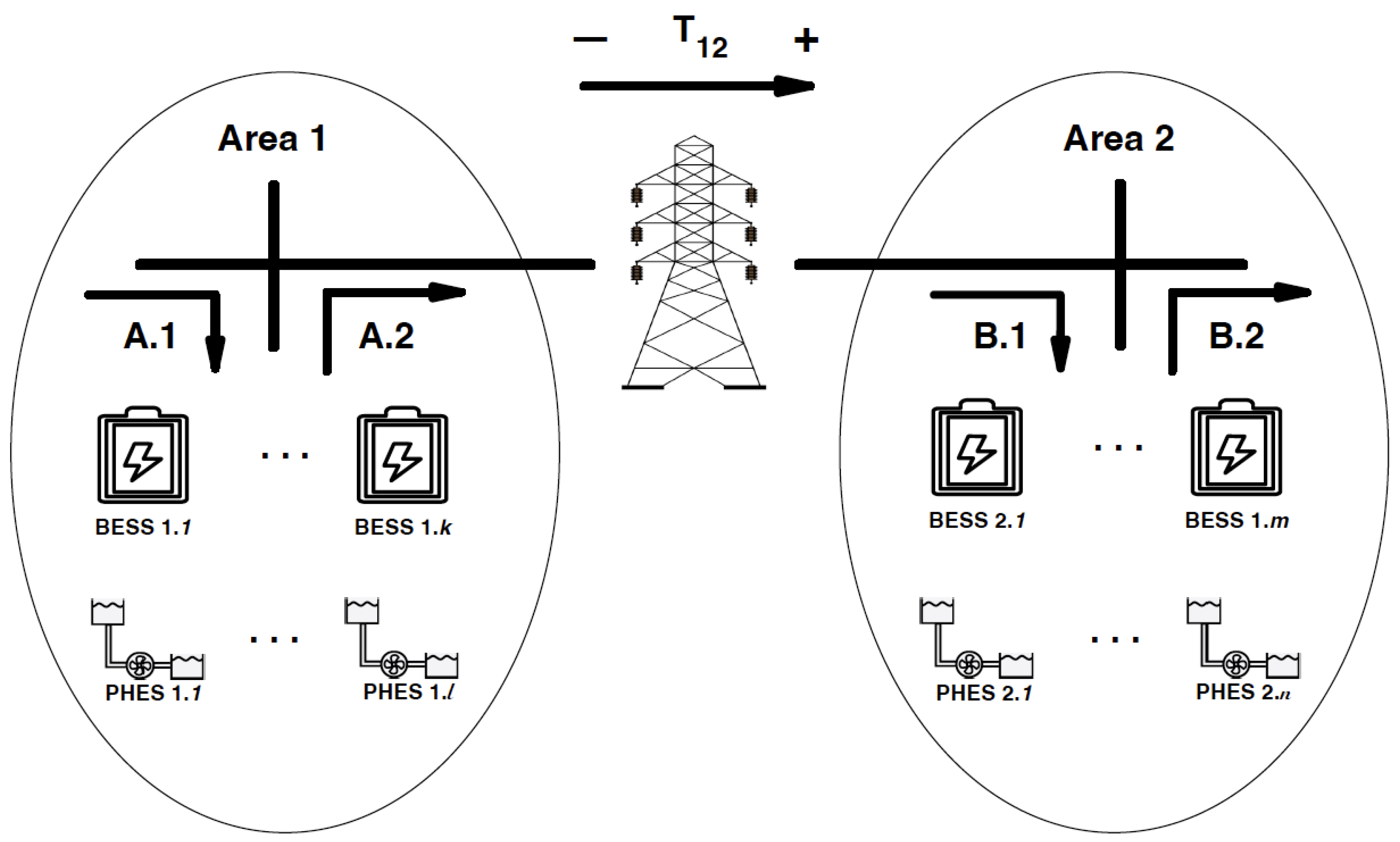
Figure 1 presents a diagram where the operation of a VTL can be illustrated, with the objective of describing the novel inter-area VTL model proposed in this work.
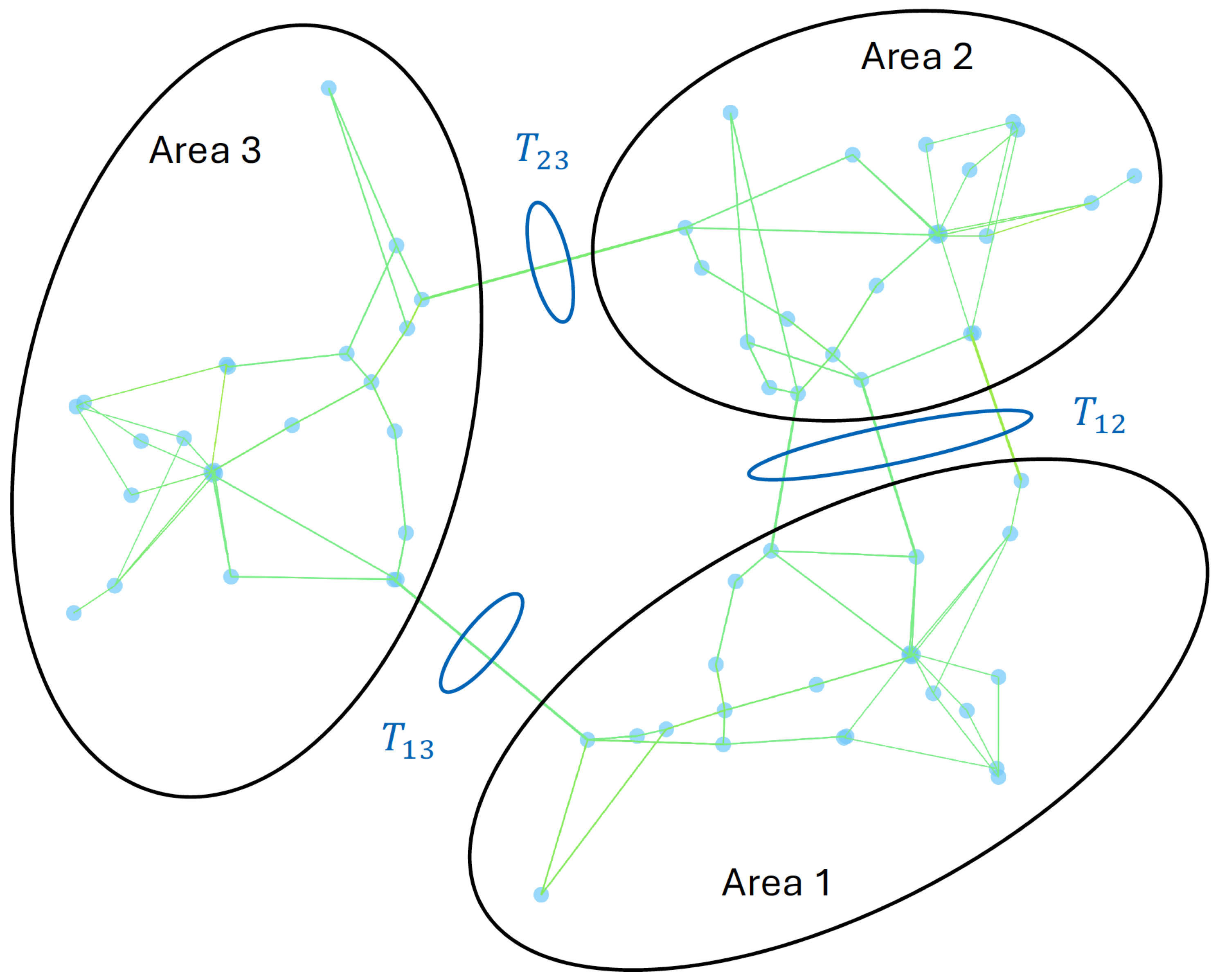
In large-scale power systems, the grid is often divided into distinct areas. An area is a geographic and operational subdivision of the whole power system. Each area can be operated by a specific operator, or areas and the whole system can be operated by a single TSO. The concept comes from the need to manage and operate large-scale interconnected grids efficiently. Transmission trunks, bundles of transmission lines linking these areas, form the backbone for inter-area power flows, effectively treating the grid as a collection of areas connected by these trunks.
Due to growing demand and VRE integration, transmission trunks can face congestion, as the distribution of regional growth among regions may, and often does, not keep pace with the distribution of regional growth in VRE use.
In the nodes of each area interconnected by a trunk, a VTL concept can be considered. In Figure 1, considering Area 1, a number of k BESSs and l PHESs are planned, and considering Area 2, a number of m BESSs and n PHESs are planned. The VTL concept can be implemented in trunk T 12 .
The operation of ESS units within the proposed VTL framework is governed by a binary logic: each group of units in a given area is either in charging mode or discharging mode at any time step, depending on the prevailing system conditions. As illustrated in Figure 2, the charging and discharging states for Area 1 storage are denoted as A.1 and A.2, respectively, while those for Area 2 are labeled B.1 and B.2.
The decision to charge or discharge the storage units in each area is driven by two primary system indicators: (i) the aggregate active power flowing through the main trunk lines at time step t during the optimization horizon, and (ii) the prevailing direction of power flow between the interconnected areas. These indicators together determine the net power transfer requirement and the required response from the storage assets.
The four possible operating states that emerge from the combination of net demand levels and trunk line power flow directions are systematically defined in Table 4, which specifies the corresponding charging or discharging action for the storage units in each situation. A detailed description of this switching logic and its implementation in the optimization model is provided in our previous work [1].
The switching logic presented in Table 4 is enforced by constraints linked to the optimization variables that govern the charging and discharging status of each ESS at every time step t during the optimization horizon. These constraints explicitly consider both the direction of power flow in the trunk and the amount of active power to be transferred at time t. The corresponding mathematical expressions that encapsulate this logic are given in Equations (8)–(18).

2.4. Virtual Power Plants

In this work, virtual power plants (VPPs) are modeled as aggregated clusters of DERs, distributed across multiple nodes of the transmission network, following the conceptual framework outlined in [66]. Each VPP is represented as a single equivalent entity with controllable power output, which is discretized into representative stages in a manner analogous to the load modeling approach described in Section 2.1.
The specific mathematical formulation, operational constraints, and integration of VPP into the GTEP model are adopted directly from our prior study [1]. There, VPPs are treated as dispatchable resources that interact with the centralized generation fleet through the shared transmission infrastructure, with their available capacity and energy provision explicitly constrained to match the contracted consumer demand. Readers are referred to that reference for the complete description of the VPP modeling approach, stage-based aggregation, and interaction with the overall expansion optimization.

2.5. Unit Commitment—Operational Flexibility Assessments

To enhance the robustness of the long-term generation expansion plan by incorporating operational flexibility assessments, a unit commitment based module is integrated into the planning model in order to evaluate the adequacy of a candidate expansion plan against key flexibility metrics, ensuring that the system can handle projected variability in net demand without excessive curtailment or flexibility deficits.
This unit-commitment-based module operates as a post-optimization validation step within the GTEP. After generating a candidate long-term expansion plan that defines new capacity additions over a multi-year horizon, the module simulates the plan’s performance under operational conditions.
The planner specifies a set of representative future daily net demand time series, selected to capture diverse scenarios such as high and low renewable penetration, seasonal variations, or forecast uncertainties. These time series can be derived from historical data or probabilistic forecasts with higher resolution to reflect real-time variability. It is important to note that this data is considered as input parameters and time series provided by the planner.
The candidate expansion plan is subjected to multiple UC simulations. For each selected net demand time series, with its relative weighting considered, flexibility metrics of the candidate GTEP are evaluated. The evaluated metrics are the following:
  • Average and maximum curtailment levels.
  • Average ramp-up surplus. The mean excess upward ramping capability (MW/h) beyond required net load ramps.
  • Average ramp-down surplus. The mean excess downward ramping capability (MW/h), to absorb drops in net load.
To address the challenges of integrating short-term operational dynamics with long-term energy planning, soft-linking emerges as a pivotal decomposition method that connects detailed power system models with comprehensive integrated energy system models. This approach facilitates the exchange of insights between high-resolution short-term simulations and broader long-term scenarios, enabling more accurate assessments of system flexibility and variability. The methodological review made in [67] provides an updated overview of such techniques, highlighting their strengths in overcoming computational limitations while preserving essential interactions across timescales.
Soft-linking refers to a decomposition approach where the subproblems are linked via relaxation or penalties applied to linking variables, rather than strict equality constraints. Subproblems can be solved independently with some control over consistency through iterative adjustments. The subproblems’ linking variables are not enforced to exactly match but are guided towards consistency via penalty functions or Lagrangian multipliers.
Consider two regions, each making investment and operational decisions, and they are connected via an interconnection with capacity (z). The goal is to coordinate their investments, but instead of hard-linking (z) (forcing both regions to have exactly the same value), we use soft-linking with a penalty ( ρ ).
min x 1 , y 1 , z 1 J 1 ( x 1 , y 1 ) + ρ ( z 1 z 2 ( k ) ) 2 ( Region 1 )
min x 2 , y 2 , z 2 J 2 ( x 2 , y 2 ) + ρ ( z 1 ( k ) z 2 ) 2 ( Region 2 )
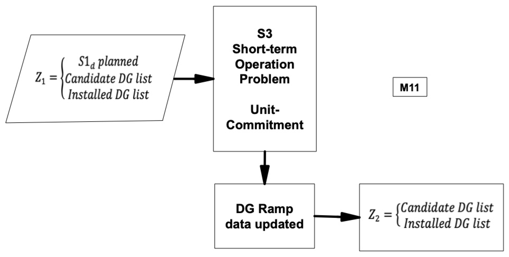
In the adopted linkage model, the interconnection variables (z) are the list of candidate and installed generators considered by the long-term level ( z 1 ), each day in which the unit commitment, the short-term level, will optimize the dispatch of generators ( z 2 ). Upon returning from the short-term level, the z 1 generators that were not considered receive an increase in their investment and operating costs proportional to the value of the current penalty; thus, these generators tend to lose investment and dispatch attractiveness. The penalty value is incremented throughout the interactions between the two levels.
From the expansion plan provided by the long-term layer, the z 1 list of candidate and installed generators related to the days that will be subject to unit commitment assessment is provided as input to the short-term layer. After processing of the unit commitment procedures, the FRUS and FRDS tables of ramp-up and ramp-down surplus are determined considering only the z 1 installed generators, and another including installed and candidate generators. An example is presented in of Section 3.
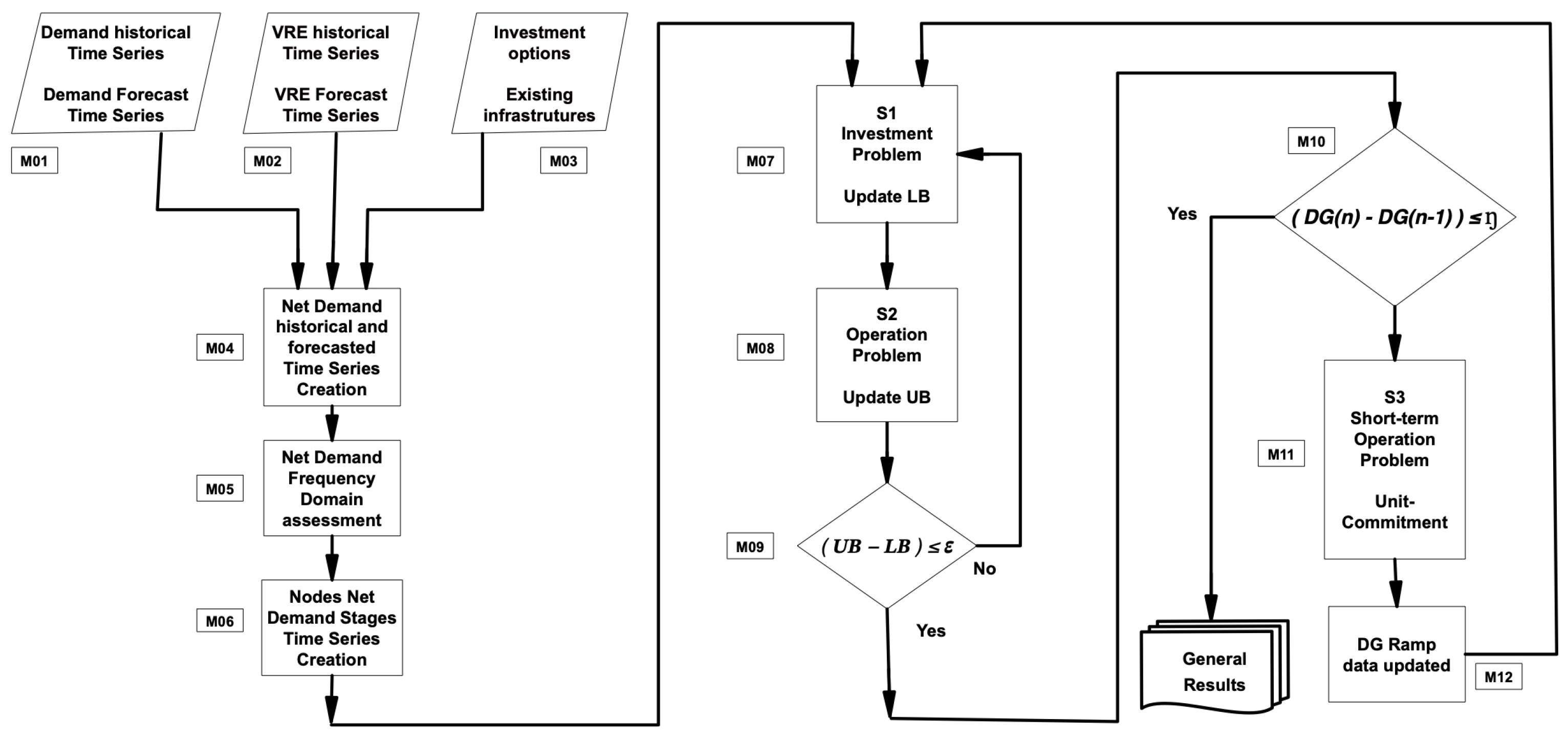
Considering the planner-defined minimum ramp-up/down surplus as a reference, the achievement of this target by the z 1 installed generator ends the planning process. If not, a penalty ρ is applied to the z 1 installed generator’s investment and operation costs, as a feedback to the long-term investment decision planning, reducing the competitiveness of these generators in relation to the candidate ones that were used for dispatch. This whole process is presented in Figure 3 and Figure 4. For each new execution of the long-term planning process, the penalty is increased. The increase rate needs to be adequately chosen considering the proportional cost difference existing between candidate generators with different flexibility indicators.

2.6. Objective Function—Investment and Operation

The objective of the proposed GTEP model is to determine the least-cost investment and operational strategy over the long-term planning horizon while satisfying demand, reliability, and flexibility constraints. In line with the deterministic optimization approach adopted in our earlier work [1], the model minimizes the present value of the total cost, which comprises annualized investment expenditures, operating costs across all time stages, load curtailment penalties, VRE curtailment costs, and additional expenses related to the unit commitment evaluation of the resulting expansion plan. The complete mathematical expression of this objective function, together with the definitions of each cost component and the discounting mechanism applied, is provided in [1]. The current study retains this formulation as the core economic criterion, extending it to incorporate the enhanced flexibility requirements and novel inter-area VTL mechanisms described herein.
The added unit commitment cost C u c is detailed in (3). It is related to higher time resolution assessment done to consider flexibility metrics related to ramp capabilities, described in Section 2.5.
C u c = n , t O C n S t B u n , t +           n , t O C n S t U s u n , t + n , t O C n S t D s d n , t + b , t O C b U L C p b , t ULC

2.7. Energy Storage System Constraints

These constraints are included to guarantee the electrical characteristics of a battery energy storage power and energy limits.
E S S h , t , w = s p h , t , s , w S T C p h , t , s , w S T D p D u r s + E S S h , t 1 , w h , t
E S S h , t , w E S S h , t , w C A P h , t
p h , t , s , w S T C s o c h , t , s , w · P h S T M a x h , t , s
p h , t , s , w S T D ( 1 s o c h , t , s , w ) · P h S T M a x h , t , s

2.8. Virtual Transmission Line Constraints

These constraints are intended to ensure coordination of energy storage systems to implement novel inter-area VTL functionality. The constraints related to ESSs are modeled according to the model proposed in [22].
f l , t , s , w S i g n 1 = f l , t , s , w
f l , t , s , w S i g n 1 V T L _ F i j 1 _ S t l , t , p , s , w · M
f l , t , s , w S i g n 1 M · 1 V T L _ F i j 1 _ S t l , t , p , s , w + V T L _ F i j 1 _ S t l , t , p , s , w · 0.001
f l , t , s , w S i g n 2 = f l , t , s , w
f l , t , s , w S i g n 2 V T L _ F i j 2 _ S t l , t , p , s , w · M
f l , t , s , w S i g n 1 M · 1 V T L _ F i j 2 _ S t l , t , p , s , w + V T L _ F i j 1 _ S t l , t , p , s , w · 0.001
V T L _ C a r g 1 _ S t l , t , s , w = P a t _ V T L _ I n d p + ( 1 V T L _ F i j 1 _ S t l , t , p ) · V T L _ F i j 2 _ S t l , t , p
V T L _ C a r g 1 _ S t l , t , s , w + P a t _ V T L _ I n d p 1 + V T L _ F i j 1 _ S t l , t , p
V T L _ C a r g 2 _ S t l , t , s , w = ( 1 V T L _ C a r g 1 _ S t l , t , s , w )
f l , t , s , w M
f l , t , s , w M
The switching logic, summarized in Table 4, is formally implemented through the constraints (8) to (18). These constraints utilize a formulation to link the binary state of the energy storage systems (ESSs)—specifically charging or discharging—to the active power flow rate stage and its direction. Flow direction is considered in constraints (8) to (13), using indicators f l , t , s , w S i g n 1 , f l , t , s , w S i g n 1 , V T L _ F i j 1 _ S t l , t , p and V T L _ F i j 2 _ S t l , t , p to capture the direction of the power flow across the trunk transmission lines. Active power flow rate is considered in constraints (14) to (16), using indicators P a t _ V T L _ I n d p , V T L _ C a r g 1 _ S t l , t , s , w ) and V T L _ C a r g 1 _ S t l , t , s , w ) to capture the active power flow rate stage.
The switching threshold is not an optimization variable. The switching logic is a function of the current power flow direction and active power flow rate stage of the transmission line as informed by the system planner. As presented in [22], which models this VPL logic, the planner defines the active power flow rate stages that are considered high transmission line usage or not. The P a t _ V T L _ I n d p parameter provides this information to constraints (14) and (15).

2.9. Flexibility Constraints

These constraints are intended to guarantee the availability of energy supply and consumption services within the limits contracted as flexibility.
P b , t , s F x D i F x D b , t . p _ m a x b FxD b , t , s
P b , t , s F x U i F x U b , t . p _ m a x b FxU b , t , s

2.10. Unit Commitment Constraints

Constraints based in [18,68] .
Status Variables
For committable generators, a binary status variable is defined:
u n , t { 0 , 1 }
where u = 1 indicates the unit is running in period t.
The power output is bounded by the status and per-unit limits
g n , t u n , t · g ̲ n , t · g ^ n
g n , t u n , t · g ¯ n , t · g ^ n
g ̲ n , t , g ¯ n , t are min/max per-unit limits, and g ^ n is nominal capacity.
Minimum Up-Time and Down-Time
t = t t + t _ m i n u p n u n , t t _ m i n u p n · ( u n , t u n , t 1 )
t = t t + t _ m i n d w n ( 1 u n , t ) t _ m i n d w n · ( u n , t 1 u n , t )
Start-Up and Shut-Down Transition Variables
Binary variables for transitions:
s u n , t { 0 , 1 } , s d n , t { 0 , 1 }
Linked to status changes:
s u n , t u n , t u n , t 1
s d n , t u n , t 1 u n , t
Ramping Constraints
For non-committable units
g n , t g n , t 1 r d n , t · g ^ n
g n , t g n , t 1 r u n , t · g ^ n
For committable units
g n , t g n , , t 1 r d n , t · u n , t r p s d n · ( u n , t 1 u n , t ) g ^ n
g n , t g n , t 1 r u n , t · u n , t 1 + r p s u n · ( u n , t u n , t 1 ) g ^ n

2.11. Inherited Model Components from Prior Work

This section outlines the foundational elements of the expansion planning model that have been retained from our prior work in [1]. These inherited components, including key variables, constraints, and assumptions, form the core framework upon which the proposed extensions are built. For comprehensive details on their formulation and rationale, readers are referred to the original publication, as they remain unmodified in the current model to ensure consistency and comparability.
The inherited components are the following constraints: power balance, demand response, reference bar and voltage, transmission line circuits, VPP and power limit constraints.

2.12. Modeling Uncertainties

The uncertainty modeling in this new expansion planning framework is inherited from our prior work [1], employing the data-driven distributionally robust optimization (DDDRO) method to identify the worst-case probability distribution across a range of ambiguities, thereby integrating elements of stochastic programming (SP) and robust optimization (RO) [35]. This approach leverages historical data to generate various scenarios, assigning worst-case probabilities supported by a moment-based ambiguity set to define the probability distribution. It formulates a two-stage robust optimization problem to ascertain the maximum cost within an uncertainty set; however, as scenario numbers increase and non-linearity emerges, computational complexity escalates, which is mitigated through a duality-free decomposition method that converts the bi-level (max–min) problem into two independent subproblems [69,70]. For a comprehensive exposition of the formulation, rationale, and implementation details, readers are directed to the original publication, as these aspects remain unaltered to maintain consistency with the foundational model.

2.13. Solution Procedure

The solution procedure for solving the proposed GTEP model with novel inter-area VTLs and enhanced flexibility constraints builds directly on the decomposition and iterative approach originally presented in our previous work [1]. While the long-term algorithmic framework is being leveraged, this new version incorporates additional steps to handle the new ramp surplus requirements, inter-area VTL coordination, and revenue stacking opportunities. The complete updated procedure, including the refined flowchart and detailed description of each stage, is presented in Figure 3 and Figure 4.
The initial steps of the solution procedure (M01–M03) focus on collecting and configuring all input parameters and network data required for determining the optimal expansion plan.
Subsequent activities (M04–M06) are devoted to constructing the lower-resolution time series that serve as inputs to the optimization phase. Load duration curves are generated, data are clustered, and representative scenarios are produced using the DDDRO approach. This method yields typical demand profiles accompanied by statistically robust uncertainty sets. Historical hourly records of load and VRE injections covering one full year are sourced from [71]. To enable a more robust application of the data-driven technique, a longer nine-year period with 15 min resolution measurements is drawn from the ENTSO-E Transparency Platform [72]. Following the partitioning strategy recommended in [73], the sample space is divided into six bins to discretize the stochastic net demand realizations and derive empirically sound probability distributions. A comprehensive account of this time series preprocessing methodology is provided in our earlier publication [1].
Step M07 performs a mixed-integer linear programming optimization to identify the binary investment decisions. Step M08 decomposes the operational optimization under uncertainty into a bi-level structure. An upper-level problem identifies the worst-case (maximum) cost within the defined uncertainty set, while the lower-level problem minimizes the expected operating cost across the individual scenarios contained in that set. To represent the uncertainty in net demand and candidate VRE injections, historical time series are discretized into data bins, from which an empirical probability distribution is derived. This empirical distribution then serves to construct a true probability distribution lying within a specified ambiguity set (tolerance band), following the DDDRO framework. The bi-level max–min problem is subsequently transformed into two decoupled single-level subproblems through the duality-free decomposition technique [69,70]. A complete description of the uncertainty modeling, binning strategy, ambiguity set construction, and duality-free reformulation is provided in our previous publication [1], where these elements were originally developed and remain unchanged in the present extension.
Finally, activities M10–M12 evaluate the expansion plan obtained from M08 by subjecting it to a detailed unit commitment assessment at higher temporal resolution. This stage quantifies the flexibility performance with respect to net demand ramps. A thorough description of these post-optimization verification steps is given in Section 2.5.

3. Results

This study evaluates the performance of the proposed GTEP model through a set of three scenarios designed to test its ability to incorporate inter-area VTLs, VPPs, distributed renewable injections, and demand-side flexibility. The model was implemented in Python 3.13.5 using the Spyder 6.0.7 IDE, Pyomo 6.9.5, and Gurobi 12.0.1 as the solver. All computations were performed on an Apple Studio M1, sourced from Apple Inc., Cupertino, CA, USA, with 64 GB RAM. Historical load and VRE generation data were obtained from the ENTSO-E Transparency Platform [72], covering the period 2015–2023 for Spain and converted to per-unit values for compatibility with the RTS-GMLC-based cases described in Section 3.1. The complete dataset of investment costs, operating parameters, and demand profiles used in this analysis is available in the public repository [74]. The case study is based on the IEEE RTS-GMLC test system [71], a well-established medium- to large-scale benchmark widely used in the literature for validating expansion planning models. Three main scenarios are analyzed to assess the model’s behavior and added value:
Scenario S1.1 (Section 3.1.1): Serves as the reference (base) case, replicating a conventional GTEP formulation with only dispatchable generation, transmission lines, and loads, as in standard literature benchmarks [71]. It provides a direct point of comparison with existing methods.
Scenario S1.2 (Section 3.1.2): Introduces candidate VTL infrastructure, utilizing realistic BESS investment and operating costs sourced from [75,76] and adjusted for PHES where applicable.
Scenario S1.3 (Section 3.1.3): Enforces a planner-defined minimum ramp-up/down surplus target to quantify the cost of explicit flexibility requirements.
All scenarios adopt a 10-year planning horizon with an assumed annual load and VRE growth rate of 4.5%. For each scenario, the resulting optimal expansion plan is summarized in dedicated tables that report the key investment and operational cost components (annualized and discounted to present value) of the minimized objective function. These summary tables allow straightforward comparison of financial outcomes and flexibility performance across cases. The decision variables optimized during the procedure form a vector of network operation and investment quantities (as listed in the Nomenclature section). These variables enter the system constraints related to power balance, equipment limits, and resource availability, and most contribute directly to the evaluation of the total cost objective that the solver minimizes to identify the economically optimal expansion solution.

3.1. IEEE RTS-GMLC

The IEEE RTS-GMLC test system is composed of 104 substation interconnections, 36 at 138 kV and 68 at 230 kV, and 16 power transformers. The RTS-GMLC also includes time series that quantify VRE injection and demands, using a one-hour time resolution for day-ahead data. For real-time data, a fifteen-minute resolution is adopted. This data is available at [71]. The Table 5 can be used to obtain a summary of the IEEE RTS-GMLC data.
The candidate ESS considered is a BESS with a maximum charge and discharge capacity of 50 MW, an efficiency of 85%, and energy storage nominal capacity of up to 75 MWh.
The IEEE RTS-GMLC is a test system dataset designed for various power system analyses, including generation and transmission expansion planning studies. The dataset provides details on the existing network topology, including buses, generators, transmission lines, transformers, reserves, storage, and time series data for loads and renewables. It does not include predefined information or data on candidate transmission lines for network expansion. In expansion planning applications using RTS-GMLC, candidate lines are typically proposed and defined separately by researchers based on their specific scenarios. Considering that in the area of transmission expansion, the focus of this research is the use of VTL applied to power flow between areas, the duplication of all trunk circuits between areas was considered as a candidate investment for transmission line expansion.
Computational performance was evaluated across the case study scenarios. On average, obtaining a solution required approximately 40 min of processing time. The most demanding instances, those involving the highest number of binary investment decisions for lines, VTL infrastructure, storage facilities, and candidate generators, took up to about 90 min to converge. These runtimes indicate that the model’s computational burden remains manageable even for medium- to large-scale networks, suggesting good scalability for practical planning applications. The IEEE RTS-GMLC system is partitioned into three generation dispatch areas, which can be leveraged to parallelize the execution of the optimization. Even without exploiting this area-based decomposition, the solution times achieved were acceptable and demonstrated robust performance on standard hardware.

3.1.1. IEEE RTS-GMLC—Scenario S1.1

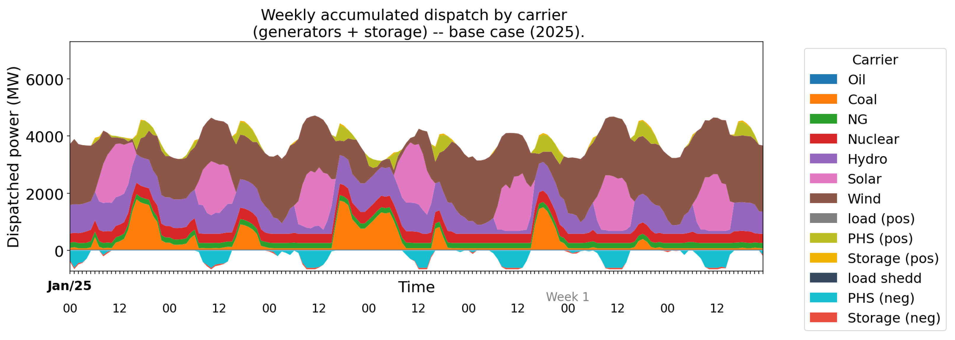
This scenario, S1.1, has the objective to be a base case for comparisons. It is considered the IEEE RTS-GMLC network with the characteristics specified and summarized in Table 5. This infrastructure, when submitted to the provided demand, provides adequate response and requires neither generation nor transmission expansion. A summary, considering a week of high demand, considering data of the defined IEEE-RTS-GMLC is presented in Figure 5.
Considering this initial infrastructure, a ten-year expansion plan was developed, projecting an annual demand growth of 4.5%.
With regard to transmission lines, the possibility of an additional circuit being considered for expansion to all existing circuits in the existing basic network was specified. Considering generation candidate expansion projects, Table 6 presents a summary of information used. Complete information can be obtained in [74].
For the results from Scenario S1.1 expansion planning, Table 7 presents candidate corridors and commissioning years. The year listed in each cell indicates the commissioning year for that line (empty cells mean no investment in that year). Table 8 presents a summary of the Scenario S1.1 expansion planning’s investment and operational costs.
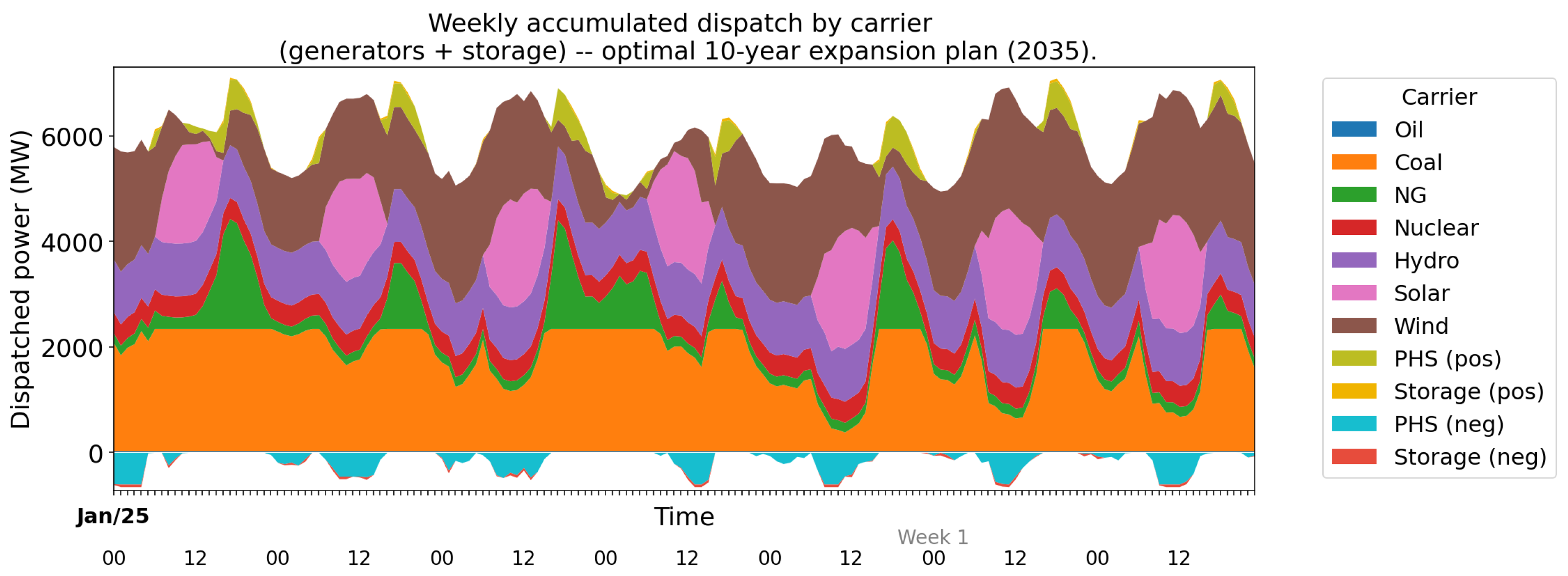
To facilitate direct comparison with established benchmarks in the literature, the base case scenario (S1.1) adopts the same modeling assumptions and objective as those employed in the reference study [71]. The resulting optimal expansion plan is fully consistent with the solutions reported in that work. A representative weekly dispatch profile during a high-demand period, extracted from the ten-year optimal plan, is illustrated in Figure 6, highlighting the alignment of generation scheduling and resource utilization with previously published results for the IEEE RTS-GMLC system.

3.1.2. IEEE RTS-GMLC—Scenario S1.2

Scenario S1.2 aims to evaluate the impact of part of the installed storage capacity and candidate storage, using a coordinated operation process to apply the VTL concept in transmission line trunks that interconnect areas of a larger transmission system. For this, the trunk of lines between Areas 3 and 2 presented in Section Virtual Transmission Lines—Revenue Stacking was chosen. Using the base scenario considered in S1.1, a 40% increase in demand in Area 2 and an equivalent increase in generation capacity installed in Area 3 were considered for S1.2. With this modification in the demand and installed generation information, expansion planning was carried out with and without the use of storage configured for VTL at the trunk of Areas 3 and 2.
For the results from Scenario S1.2 expansion planning, without VTL investments, Table 9 presents candidate corridors and commissioning years. The year listed in each cell indicates the commissioning year for that line (empty cells mean no investment in that year). Table 10 presents a summary of the scenario S1.2 expansion planning’s investment and operational costs.
For the results from Scenario S1.2 expansion planning, considering VTL investments, Table 11 presents candidate corridors and commissioning years. The year listed in each cell indicates the commissioning year for that line (empty cells mean no investment in that year). Table 12 presents a summary of the Scenario S1.2 expansion planning’s investment and operational costs.
The results obtained show the positive impact on the quality of the expansion plan achieved through optimized investment in storage allocation in the two areas involved. It was possible to reduce investments in transmission line expansion and achieve more optimized use, which can be seen in generation expenses.
As shown in the comparison between the expansion plans in Section 3.1.2 (specifically comparing Table 10 and Table 12), the annual saving of approximately 2.5% stems from three primary areas:
  • Generation investment reduction (35.11 MUSD/year): This constitutes the largest portion of the savings. The strategic allocation of the ESS for VTL services allows the system to optimize the generation portfolio more efficiently, reducing the overall requirement for new candidate generation capacity.
  • Network investment reduction/transmission deferral (2.03 MUSD/year): By utilizing the inter-area VTL to increase the effective power transfer capacity of existing trunks, the model successfully reduces the need for capital-intensive physical transmission line expansions. The trunk of lines between Areas 3 and 2 that was chosen (N_318 N_223), without candidate VTL ESS, needed expansion in 2026 for two circuits, as shown in Table 9. Considering the investment in VTL in this trunk line, expansion was postponed to 2030 (first circuit) and 2031 (second circuit), as shown in Table 11.
  • Operation cost reduction (4.71 MUSD/year): The VTL logic improves operational efficiency by mitigating inter-area congestion. This leads to reduced redispatch and minimizes the curtailment of low-cost renewable energy, thereby lowering daily generation operating expenses.
These results demonstrate that the inter-area VTL not only defers conventional grid and generation investments but also optimizes the utilization of the entire system, providing a robust economic justification for localized storage deployment.

3.1.3. IEEE RTS-GMLC—Scenario S1.3

Different technologies and generations of power generation technologies have their own parameter ranges related to ramp-up and ramp-down flexibility indicators. Table 13 presents a summary considering the various values used in published case studies that reference the IEEE RTS-GMLC network. The ratio represents the time in hours to reach nominal power, calculated as 100/(60×ramp rate %/min). The values are approximated based on typical ranges for each technology. For gas, an average between open-cycle gas turbines (OCGTs) (around 10–12%) and combined-cycle gas turbines (CCGTs) (around 4–8%) is used, but with a tendency towards OCGTs at the former value. For nuclear power, the values are based on modern PWR capacities. For oil, the approximation is similar to that of flexible thermal power plants.
Scenario S1.3 considers a projected increase in ramp-up/down surplus flexibility metric, as a parameter provided by the planner. Initially, the expansion plan generated from the base case was used, without using the third step in which, based on the planner’s parameter, a minimum ramp-up and down surplus is defined. The results of the expansion plan obtained, without considering the minimum ramp-up and down surplus flexibility metric, are presented in Table 14.
Similarly to the results presented for the ramp-up surplus metric, the result for the ramp-down surplus metric is an average equal to 0.354 MW/h.
The ramp-up surplus and ramp-down surplus flexibility indicator of a power generation and transmission system is useful for assessing how flexible a system is for withstanding uncertainties in net demand ramps during operation. With the data used and projected for 10 years of the IEEE RTS-GMLC system, the value of the average net demand ramp met per generator in the worst case reaches 12.1 MW/h. With generator utilization considering only the optimal power flow, the system has an average ramp-up surplus indicator per generator of 0.354 MW/h. Using the proposed expansion model, expansion plans were proposed indicating, as planner specified, three possibilities of minimum ramp-up and ramp-down surplus targets of 0.5, 1.5, and 2 MW/h. The 2 MW/h target with the installed and candidate generators was infeasible given the current candidate generator set. Table 15 and Table 16 summarize the results of the expansion plan with the 1.5 MW/h target.
To validate the functionality of the model’s third level, an example target of a minimum average value of 1.5 MW/h for ramp-up or ramp-down was defined, using the initial baseline scenario. The results of the expansion plan obtained, considering the flexibility metric of the minimum ramp-up and ramp-down surplus, are presented in Table 15.
Similarly to the results presented for the ramp-up surplus metric, the result for the ramp-down surplus metric is an average equal to 1.547 MW/h.
The evaluation of Scenario S1.3, Table 16 demonstrates that imposing a minimum average ramp-up (and symmetrically ramp-down) surplus requirement of 1.5 MW/h significantly enhances system flexibility, increasing the average ramp-up surplus from 0.354 MW/h (base case without constraint) to 1.547 MW/h (constrained case). This flexibility gain comes at a moderate economic cost: the total annual expansion cost rises from 1663.95 M US$/year to 1680.35 M US$/year, corresponding to an increase of approximately 16.4 M US$/year (+0.99%). The additional cost is primarily driven by higher generation investment (increase of 5.94 M US$/year) and network investment (increase of 1.28 M US$/year), along with elevated generation operation costs (increase of 9.17 M US$/year), while energy not supplied (ENS) remains zero in both cases. These results highlight a clear trade-off between improved operational flexibility, particularly valuable under high variable renewable energy penetration, and modest increases in long-term planning costs, underscoring the value of explicitly incorporating ramping adequacy constraints in generation-transmission expansion models.

4. Conclusions

This article has introduced a novel optimization model for dynamic multi-period GTEP that builds upon our prior work by introducing a novel inter-area VTL framework through strategic allocation of ESS across multiple network areas. This new model enables the optimization of trunk transmission lines connecting these areas, facilitating potential postponements or reductions in expansion investments while maintaining system reliability and efficiency. Additionally, the model incorporates a third optimization level employing UC procedures to achieve finer temporal resolution, thereby better accommodating ramping resources required to address the uncertainties and variabilities in net demand driven by VRE integration.
In summary, the proposed model advances the state of the art in integrated generation-transmission-storage expansion planning by introducing three original contributions that, to the authors’ knowledge, have not been previously addressed in the literature: the new booster inter-area virtual transmission line concept with revenue stacking, the endogenous treatment of flexibility metrics in dynamic planning, and a consistent three-level optimization framework bridging investment, operation, and unit commitment. These developments provide a more comprehensive and flexible tool for planning future power systems with high shares of variable renewables and storage.
The proposed formulation retains core elements from the original model, including a linear AC optimal power flow (AC-OPF) with reactive power considerations, flexibility provisioning from TSO-DSO interconnections via aggregated VPPs, and a DDDRO approach to handle demand and VRE uncertainties. To ensure computational tractability for medium to large systems, the model employs a two-level architecture based on the column-and-constraint generation (CCG) algorithm and duality-free decomposition, now augmented by the UC level for enhanced ramping and flexibility constraints. Flexibility metrics are carefully selected to quantify short-term operational resources, with required levels derived from distribution system operator (DSO) planning and supplied to the transmission network.
The new model was validated through case studies on the IEEE RTS-GMLC test system, demonstrating its effectiveness in real-world scenarios. Results indicate significant benefits. The introduction of the inter-area VTL yields clear economic advantages, as evidenced by the comparison between the two solutions. When the inter-area VTL is employed, the total annual cost decreases from 1805.80 M US$ (without VTL) to 1763.95 M US$, representing a reduction of approximately 41.85 M US$ per year (≈2.5%). This overall saving stems from lower investment costs in both generation (reduction of 35.11 M US$) and network infrastructure (reduction of 2.03 M US$), combined with decreased generation operating costs (saving of 4.71 M US$), while maintaining zero energy not supplied (ENS) cost in both cases. These results demonstrate that the inter-area VTL not only defers or reduces conventional grid and generation investments but also improves operational efficiency, delivering substantial cost savings without compromising system reliability. Furthermore, the approach yields enhanced transmission system utilization efficiency and improved congestion indicators, underscoring the value of localized ESS deployment and high-resolution UC in mitigating expansion needs.
Beyond the direct cost reductions observed in the planning model, the adoption of inter-area virtual transmission lines offers additional financial upside through revenue stacking opportunities. Because the energy storage systems deployed for VTL operation exhibit dynamic duty cycles, with significant periods of partial or zero utilization for congestion relief, their remaining capacity can be actively marketed in ancillary services markets (e.g., frequency regulation, spinning reserves, voltage support) and energy arbitrage. These secondary revenue streams, not yet quantified in the present GTEP results, would further improve the overall return on investment of the storage assets and accelerate the economic justification for deferring conventional network and generation expansions. Preliminary industry benchmarks suggest that well-coordinated multi-service operation can increase the net present value of utility-scale BESS, depending on market conditions, thereby enhancing the attractiveness of the proposed VTL approach in expansion planning studies.
Overall, this work advances the design of modern, low-carbon power systems by promoting the integration of advanced storage technologies and flexible resources, offering a robust framework for planners to balance economic, operational, and environmental objectives in an era of increasing renewable penetration. Future research could explore integrated models that couple GTEP with expansion planning of other energy infrastructures, such as natural gas networks and hydrogen systems, to optimize cross-sector synergies and support broader energy transition goals.

Author Contributions

Conceptualization, F.A.L.F.; Methodology, F.A.L.F. and C.U.V.; Software, F.A.L.F.; Validation, F.A.L.F. and C.U.V.; Formal analysis, F.A.L.F. and C.U.V.; Investigation, F.A.L.F.; Resources, F.A.L.F.; Writing—original draft, F.A.L.F.; Writing—review & editing, F.A.L.F. and C.U.V.; Visualization, F.A.L.F.; Supervision, C.U.V.; Project administration, F.A.L.F.; Funding acquisition, F.A.L.F. All authors have read and agreed to the published version of the manuscript.

Funding

This research received no external funding.

Data Availability Statement

The original data presented in the study are openly available in [74].

Conflicts of Interest

The authors declare no conflicts of interest.

Nomenclature

The nomenclature (sets, indices, parameters, and variables) used in this work largely follows that introduced in our previous publication [1]. For the complete list of symbols and definitions common to both papers, the reader is referred to [1]. Only the new or significantly modified items introduced in this extension (primarily related to unit commitment, ramping constraints, and inter-area virtual transmission elements) are listed below.
Unit Commitment—Input Data—Parameters
r u n , t Ramp-up capacity of generator
r d n , t Ramp-down capacity of generator
r p s u n Ramp limit start up of generator
r p s d n Ramp limit shut down of generator
g ̲ n , s , t Min per-unit limit of generator
g ¯ n , s , t Max per-unit limit of generator
g ^ n , s Nominal capacity of generator
t _ m i n u p n Min time up of generator
t _ m i n d w n Min time down of generator
g ̲ n , t Min per-unit limit of generator
g ¯ n , t Max per-unit limit of generator
g ^ n Min nominal capacity of generator
O C n S t B Stand-by cost of generator n in time period t [$/ h ]
O C n S t U Start-up cost of generator n in time period t [$/event ]
O C n S t D Start-down cost of generator n in time period t [$/event]
O C b U L C Variable cost of UC load curtailment at node b [$/ M W h ]
Unit Commitment—Decision Variables
u n , t Binary variable indicating if generator is dispatched
s u n , t Binary variable indicating if generator is start up
s d n , t Binary variable indicating if generator is shut down
g n , t Dispatch power of generator
p b , t ULC          Active power of UC curtailed demand, bus b, time period t

References

  1. Ferreira, F.A.L.; Unsihuay-Vila, C.; Núñez-Rodríguez, R.A. Transmission and Generation Expansion Planning Considering Virtual Power Lines/Plants, Distributed Energy Injection and Demand Response Flexibility from TSO-DSO Interface. Energies 2025, 18, 1602. [Google Scholar] [CrossRef]
  2. Lindner, M.; Peper, J.; Offermann, N.; Biele, C.; Teodosic, M.; Pohl, O.; Menne, J.; Häger, U. Operation strategies of battery energy storage systems for preventive and curative congestion management in transmission grids. IET Gener. Transm. Distrib. 2023, 17, 589–603. [Google Scholar] [CrossRef]
  3. Agüero, M.; Peralta, J.; Quintana, E.; Velar, V.; Stepanov, A.; Ashourian, H.; Mahseredjian, J.; Cárdenas, R. Virtual Transmission Solution Based on Battery Energy Storage Systems to Boost Transmission Capacity. J. Mod. Power Syst. Clean Energy 2024, 12, 466–474. [Google Scholar] [CrossRef]
  4. Wang, Q.; Li, X. Evaluation of battery energy storage system to provide virtual transmission service. Electr. Power Syst. Res. 2025, 244, 111570. [Google Scholar] [CrossRef]
  5. Latorre, G.; Cruz, R.D.; Areiza, J.M.; Villegas, A. Classification of publications and models on transmission expansion planning. IEEE Trans. Power Syst. 2003, 18, 938–946. [Google Scholar] [CrossRef]
  6. Hemmati, R.; Hooshmand, R.; Khodabakhshian, A. Comprehensive review of generation and transmission expansion planning. IET Gener. Transm. Distrib. 2013, 7, 955–964. [Google Scholar] [CrossRef]
  7. Mahdavi, M.; Sabillon Antunez, C.; Ajalli, M.; Romero, R. Transmission Expansion Planning: Literature Review and Classification. IEEE Syst. J. 2019, 13, 3129–3140. [Google Scholar] [CrossRef]
  8. Muralikrishnan, N.; Jebaraj, L.; Rajan, C.C.A. A Comprehensive Review on Evolutionary Optimization Techniques Applied for Unit Commitment Problem. IEEE Access 2020, 8, 132980–133014. [Google Scholar] [CrossRef]
  9. Ali, A.; Shah, A.; Keerio, M.U.; Mugheri, N.H.; Abbas, G.; Touti, E.; Hatatah, M.; Yousef, A.; Bouzguenda, M. Multi-Objective Security Constrained Unit Commitment via Hybrid Evolutionary Algorithms. IEEE Access 2024, 12, 6698–6718. [Google Scholar] [CrossRef]
  10. Tejada-Arango, D.A.; Morales-España, G.; Wogrin, S.; Centeno, E. Power-Based Generation Expansion Planning for Flexibility Requirements. IEEE Trans. Power Syst. 2020, 35, 2012–2023. [Google Scholar] [CrossRef]
  11. Han, T.; Hill, D.J.; Song, Y. Optimal Transmission Switching With Uncertainties From Both Renewable Energy and N-K Contingencies. IEEE Trans. Sustain. Energy 2023, 14, 1964–1978. [Google Scholar] [CrossRef]
  12. Palmintier, B.S.; Webster, M.D. Impact of Operational Flexibility on Electricity Generation Planning With Renewable and Carbon Targets. IEEE Trans. Sustain. Energy 2016, 7, 672–684. [Google Scholar] [CrossRef]
  13. Chen, X.; Lv, J.; McElroy, M.B.; Han, X.; Nielsen, C.P.; Wen, J. Power System Capacity Expansion Under Higher Penetration of Renewables Considering Flexibility Constraints and Low Carbon Policies. IEEE Trans. Power Syst. 2018, 33, 6240–6253. [Google Scholar] [CrossRef]
  14. Liu, X.; Fang, X.; Gao, N.; Yuan, H.; Hoke, A.; Wu, H.; Tan, J. Frequency Nadir Constrained Unit Commitment for High Renewable Penetration Island Power Systems. IEEE Open Access J. Power Energy 2024, 11, 141–153. [Google Scholar] [CrossRef]
  15. Chen, X.; Liu, Y.; Wu, L. Towards Improving Unit Commitment Economics: An Add-On Tailor for Renewable Energy and Reserve Predictions. IEEE Trans. Sustain. Energy 2024, 15, 2547–2566. [Google Scholar] [CrossRef]
  16. Backe, S.; Ahang, M.; Tomasgard, A. Stable stochastic capacity expansion with variable renewables: Comparing moment matching and stratified scenario generation sampling. Appl. Energy 2021, 302, 117538. [Google Scholar] [CrossRef]
  17. Wuijts, R.H.; van den Akker, M.; van den Broek, M. Effect of modelling choices in the unit commitment problem. Energy Syst. 2024, 15, 1–63. [Google Scholar] [CrossRef]
  18. Ramos, A.; Alvarez, E.F.; Lumbreras, S. OpenTEPES: Open-source Transmission and Generation Expansion Planning. SoftwareX 2022, 18, 101070. [Google Scholar] [CrossRef]
  19. Curty, M.G.; Borges, C.L.; Saboia, C.H.; Lisboa, M.L.; Berizzi, A. A soft-linking approach to include hourly scheduling of intermittent resources into hydrothermal generation expansion planning. Renew. Sustain. Energy Rev. 2023, 188, 113838. [Google Scholar] [CrossRef]
  20. Yin, X.; Chen, H.; Liang, Z.; Zhu, Y. A Flexibility-oriented robust transmission expansion planning approach under high renewable energy resource penetration. Appl. Energy 2023, 351, 121786. [Google Scholar] [CrossRef]
  21. Ghaljehei, M.; Khorsand, M. Day-Ahead Operational Scheduling with Enhanced Flexible Ramping Product: Design and Analysis. IEEE Trans. Power Syst. 2022, 37, 1842–1856. [Google Scholar] [CrossRef]
  22. Xu, B.; Oudalov, A.; Ulbig, A.; Andersson, G.; Kirschen, D.S. Modeling of Lithium-Ion Battery Degradation for Cell Life Assessment. IEEE Trans. Smart Grid 2018, 9, 1131–1140. [Google Scholar] [CrossRef]
  23. Xiong, L.; Huang, S.; Li, P.; Wang, Z.; Khan, M.W.; Niu, T. Hidden Markov Jump System Based Robust Control of Inverter-Fed Power Systems With Asynchronous Sliding Mode Observer. IEEE Trans. Ind. Electron. 2025, 72, 13287–13299. [Google Scholar] [CrossRef]
  24. Xiong, L.; Li, T.; Huang, S.; Li, P.; Wang, Z.; Sun, Z.; Niu, T. Optimized Sizing of ESSs in Non-Array Formed Wind Farm for Frequency Support Considering Multi-Directional Wake Effect. IEEE Trans. Sustain. Energy 2025, 17, 1878–1893. [Google Scholar] [CrossRef]
  25. Dehghan, S.; Amjady, N.; Conejo, A.J. A Multistage Robust Transmission Expansion Planning Model Based on Mixed Binary Linear Decision Rules—Part I. IEEE Trans. Power Syst. 2018, 33, 5341–5350. [Google Scholar] [CrossRef]
  26. Zhang, H.; Heydt, G.T.; Vittal, V.; Quintero, J. An Improved Network Model for Transmission Expansion Planning Considering Reactive Power and Network Losses. IEEE Trans. Power Syst. 2013, 28, 3471–3479. [Google Scholar] [CrossRef]
  27. Ghaddar, B.; Jabr, R.A. Power transmission network expansion planning: A semidefinite programming branch-and-bound approach. Eur. J. Oper. Res. 2019, 274, 837–844. [Google Scholar] [CrossRef]
  28. Mehrtash, M.; Cao, Y. A New Global Solver for Transmission Expansion Planning with AC Network Model. IEEE Trans. Power Syst. 2022, 37, 282–293. [Google Scholar] [CrossRef]
  29. Mehrtash, M.; Hobbs, B.F.; Mahroo, R.; Cao, Y. Does Choice of Power Flow Representation Matter in Transmission Expansion Optimization? A Quantitative Comparison for a Large-Scale Test System. IEEE Trans. Ind. Appl. 2024, 60, 1433–1441. [Google Scholar] [CrossRef]
  30. Wendelborg, M.A.; Backe, S.; del Granado, P.C.; Seifert, P.E. Consequences of Uncertainty from Intraday Operations to a Capacity Expansion Model of the European Power System. In Proceedings of the 2023 19th International Conference on the European Energy Market (EEM); IEEE: New York, NY, USA, 2023; pp. 1–8. [Google Scholar] [CrossRef]
  31. Domínguez, R.; Conejo, A.J.; Carrión, M. Toward Fully Renewable Electric Energy Systems. IEEE Trans. Power Syst. 2015, 30, 316–326. [Google Scholar] [CrossRef]
  32. Baringo, L.; Baringo, A. A Stochastic Adaptive Robust Optimization Approach for the Generation and Transmission Expansion Planning. IEEE Trans. Power Syst. 2018, 33, 792–802. [Google Scholar] [CrossRef]
  33. Moreira, A.; Pozo, D.; Street, A.; Sauma, E. Reliable Renewable Generation and Transmission Expansion Planning: Co-Optimizing System’s Resources for Meeting Renewable Targets. IEEE Trans. Power Syst. 2017, 32, 3246–3257. [Google Scholar] [CrossRef]
  34. Ranjbar, H.; Hosseini, S.H.; Zareipour, H. A robust optimization method for co-planning of transmission systems and merchant distributed energy resources. Int. J. Electr. Power Energy Syst. 2020, 118, 105845. [Google Scholar] [CrossRef]
  35. Zhang, C.; Liu, L.; Cheng, H.; Liu, D.; Zhang, J.; Li, G. Data-driven distributionally robust transmission expansion planning considering contingency-constrained generation reserve optimization. Int. J. Electr. Power Energy Syst. 2021, 131, 106973. [Google Scholar] [CrossRef]
  36. Ranjbar, H.; Hosseini, S.H.; Zareipour, H. Resiliency-Oriented Planning of Transmission Systems and Distributed Energy Resources. IEEE Trans. Power Syst. 2021, 36, 4114–4125. [Google Scholar] [CrossRef]
  37. Abushamah, H.A.S.; Haghifam, M.; Bolandi, T.G. A novel approach for distributed generation expansion planning considering its added value compared with centralized generation expansion. Sustain. Energy, Grids Netw. 2021, 25, 100417. [Google Scholar] [CrossRef]
  38. Ahmadi, S.; Mavalizadeh, H.; Ghadimi, A.A.; Miveh, M.R.; Ahmadi, A. Dynamic robust generation–transmission expansion planning in the presence of wind farms under long- and short-term uncertainties. IET Gener. Transm. Distrib. 2020, 14, 5418–5427. [Google Scholar] [CrossRef]
  39. Moreira, A.; Pozo, D.; Street, A.; Sauma, E.; Strbac, G. Climate-aware generation and transmission expansion planning: A three-stage robust optimization approach. Eur. J. Oper. Res. 2021, 295, 1099–1118. [Google Scholar] [CrossRef]
  40. El-Meligy, M.A.; Sharaf, M.; Soliman, A.T. A coordinated scheme for transmission and distribution expansion planning: A Tri-level approach. Electr. Power Syst. Res. 2021, 196, 107274. [Google Scholar] [CrossRef]
  41. Toolabi Moghadam, A.; Bahramian, B.; Shahbaazy, F.; Paeizi, A.; Senjyu, T. Stochastic Flexible Power System Expansion Planning, Based on the Demand Response Considering Consumption and Generation Uncertainties. Sustainability 2023, 15, 1099. [Google Scholar] [CrossRef]
  42. García-Bertrand, R.; Mínguez, R. Dynamic Robust Transmission Expansion Planning. IEEE Trans. Power Syst. 2017, 32, 2618–2628. [Google Scholar] [CrossRef]
  43. Roldán, C.; Mínguez, R.; García-Bertrand, R.; Arroyo, J.M. Robust Transmission Network Expansion Planning Under Correlated Uncertainty. IEEE Trans. Power Syst. 2019, 34, 2071–2082. [Google Scholar] [CrossRef]
  44. Liang, Z.; Chen, H.; Chen, S.; Wang, Y.; Zhang, C.; Kang, C. Robust Transmission Expansion Planning Based on Adaptive Uncertainty Set Optimization Under High-Penetration Wind Power Generation. IEEE Trans. Power Syst. 2021, 36, 2798–2814. [Google Scholar] [CrossRef]
  45. Liang, Z.; Chen, H.; Chen, S.; Lin, Z.; Kang, C. Probability-driven transmission expansion planning with high-penetration renewable power generation: A case study in northwestern China. Appl. Energy 2019, 255, 113610. [Google Scholar] [CrossRef]
  46. Yin, X.; Chen, H.; Liang, Z.; Zeng, X.; Zhu, Y.; Chen, J. Robust transmission network expansion planning based on a data-driven uncertainty set considering spatio-temporal correlation. Sustain. Energy, Grids Netw. 2023, 33, 100965. [Google Scholar] [CrossRef]
  47. Garcia-Cerezo, A.; Baringo, L.; Garcia-Bertrand, R. Dynamic Robust Transmission Network Expansion Planning in Renewable Dominated Power Systems Considering Inter-Temporal and Non-Convex Operational Constraints. In Proceedings of the 2022 International Conference on Smart Energy Systems and Technologies (SEST); IEEE: New York, NY, USA, 2022; pp. 1–6. [Google Scholar] [CrossRef]
  48. Garcia-Cerezo, A.; Baringo, L.; Garcia-Bertrand, R. Expansion planning of the transmission network with high penetration of renewable generation: A multi-year two-stage adaptive robust optimization approach. Appl. Energy 2023, 349, 121653. [Google Scholar] [CrossRef]
  49. Zhang, X.; Conejo, A.J. Coordinated Investment in Transmission and Storage Systems Representing Long- and Short-Term Uncertainty. IEEE Trans. Power Syst. 2018, 33, 7143–7151. [Google Scholar] [CrossRef]
  50. Verastegui, F.; Lorca, A.; Olivares, D.E.; Negrete-Pincetic, M.; Gazmuri, P. An Adaptive Robust Optimization Model for Power Systems Planning With Operational Uncertainty. IEEE Trans. Power Syst. 2019, 34, 4606–4616. [Google Scholar] [CrossRef]
  51. Li, J.; Li, Z.; Liu, F.; Ye, H.; Zhang, X.; Mei, S.; Chang, N. Robust Coordinated Transmission and Generation Expansion Planning Considering Ramping Requirements and Construction Periods. IEEE Trans. Power Syst. 2018, 33, 268–280. [Google Scholar] [CrossRef]
  52. Taibi, E.; Nikolakakis, T.; Gutierrez, L.; Fernandez del Valle, C.; Kiviluoma, J.; Lindroos, T.; Rissanen, S. Power System Flexibility for the Energy Transition; IRENA Flextool Methodology; IRENA International Renewable Energy: Masdar, United Arab Emirates, 2018. [Google Scholar] [CrossRef]
  53. Cochran, J.; Miller, M.; Zinaman, O.; Milligan, M.; Arent, D.; Palmintier, B.; O’Malley, M.; Mueller, S.; Lannoye, E.; Tuohy, A.; et al. Flexibility in 21st Century Power Systems; Technical Report; National Renewable Energy Lab. (NREL): Golden, CO, USA, 2014. [Google Scholar]
  54. Cañas-Carretón, M.; Carrión, M. Generation Capacity Expansion Considering Reserve Provision by Wind Power Units. IEEE Trans. Power Syst. 2020, 35, 4564–4573. [Google Scholar] [CrossRef]
  55. Huber, M.; Dimkova, D.; Hamacher, T. Integration of wind and solar power in Europe: Assessment of flexibility requirements. Energy 2014, 69, 236–246. [Google Scholar] [CrossRef]
  56. Ringkjøb, H.K.; Haugan, P.M.; Seljom, P.; Lind, A.; Wagner, F.; Mesfun, S. Short-term solar and wind variability in long-term energy system models—A European case study. Energy 2020, 209, 118377. [Google Scholar] [CrossRef]
  57. O’Sullivan, J.; Rogers, A.; Flynn, D.; Smith, P.; Mullane, A.; O’Malley, M. Studying the Maximum Instantaneous Non-Synchronous Generation in an Island System—Frequency Stability Challenges in Ireland. IEEE Trans. Power Syst. 2014, 29, 2943–2951. [Google Scholar] [CrossRef]
  58. Fonseca, N.; Neyestani, N.; Soares, F.; Iria, J.; Lopes, M.; Antunes, C.H.; Pinto, D.; Jorge, H. Bottom-up approach to compute der flexibility in the transmission-distribution networks boundary. In Proceedings of the Mediterranean Conference on Power Generation, Transmission, Distribution and Energy Conversion (MEDPOWER 2018); IET: Stevenage, UK, 2018; pp. 1–7. [Google Scholar] [CrossRef]
  59. Rahman, M.M.; Dadon, S.H.; He, M.; Giesselmann, M.; Hasan, M.M. An Overview of Power System Flexibility: High Renewable Energy Penetration Scenarios. Energies 2024, 17, 6393. [Google Scholar] [CrossRef]
  60. Yurdakul, O.; Ela, E.; Billimoria, F. Flexible Ramping Product Procurement in Day-Ahead Markets. IEEE Trans. Energy Mark. Policy Regul. 2025, 3, 13–31. [Google Scholar] [CrossRef]
  61. Hurtado, M.; Jafarian, M.; Kërçi, T.; Tweed, S.; Escudero, M.V.; Kennedy, E.; Milano, F. Stability Assessment of Low-Inertia Power Systems: A System Operator Perspective. In Proceedings of the 2024 IEEE Power & Energy Society General Meeting (PESGM); IEEE: New York, NY, USA, 2024; pp. 1–5. [Google Scholar] [CrossRef]
  62. Mohamed, A.A.R.; Best, R.J.; Liu, X.; Morrow, D.J.; Pollock, J.; Cupples, A. Stacking Battery Energy Storage Revenues in Future Distribution Networks. IEEE Access 2022, 10, 35026–35039. [Google Scholar] [CrossRef]
  63. Nguyen, T.A.; Copp, D.A.; Byrne, R.H. Stacking Revenue from Energy Storage Providing Resilience, T & D Deferral and Arbitrage. In Proceedings of the 2019 IEEE Power & Energy Society General Meeting (PESGM); IEEE: New York, NY, USA, 2019; pp. 1–5. [Google Scholar] [CrossRef]
  64. Steriotis, K.; Šepetanc, K.; Smpoukis, K.; Efthymiopoulos, N.; Makris, P.; Varvarigos, E.; Pandžić, H. Stacked Revenues Maximization of Distributed Battery Storage Units Via Emerging Flexibility Markets. IEEE Trans. Sustain. Energy 2022, 13, 464–478. [Google Scholar] [CrossRef]
  65. Pocola, T.O.; Robu, V.; Rietveld, J.; Norbu, S.; Couraud, B.; Andoni, M.; Flynn, D.; Poor, H. Optimal sizing and control of a grid-connected battery in a stacked revenue model including an energy community. Appl. Energy 2025, 397, 126122. [Google Scholar] [CrossRef]
  66. Baringo, A.; Baringo, L.; Arroyo, J.M. Holistic planning of a virtual power plant with a nonconvex operational model: A risk-constrained stochastic approach. Int. J. Electr. Power Energy Syst. 2021, 132, 107081. [Google Scholar] [CrossRef]
  67. Collins, S.; Deane, J.P.; Poncelet, K.; Panos, E.; Pietzcker, R.C.; Delarue, E.; Ó Gallachóir, B. Integrating short term variations of the power system into integrated energy system models: A methodological review. Renew. Sustain. Energy Rev. 2017, 76, 839–856. [Google Scholar] [CrossRef]
  68. Hua, B.; Baldick, R.; Wang, J. Representing Operational Flexibility in Generation Expansion Planning Through Convex Relaxation of Unit Commitment. IEEE Trans. Power Syst. 2018, 33, 2272–2281. [Google Scholar] [CrossRef]
  69. Ding, T.; Yang, Q.; Liu, X.; Huang, C.; Yang, Y.; Wang, M.; Blaabjerg, F. Duality-Free Decomposition Based Data-Driven Stochastic Security-Constrained Unit Commitment. IEEE Trans. Sustain. Energy 2019, 10, 82–93. [Google Scholar] [CrossRef]
  70. Wang, L.; Jiang, C.; Gong, K.; Si, R.; Shao, H.; Liu, W. Data-driven distributionally robust economic dispatch for distribution network with multiple microgrids. IET Gener. Transm. Distrib. 2020, 14, 5712–5719. [Google Scholar] [CrossRef]
  71. Barrows, C.; Bloom, A.; Ehlen, A.; Ikäheimo, J.; Jorgenson, J.; Krishnamurthy, D.; Lau, J.; McBennett, B.; O’Connell, M.; Preston, E.; et al. The IEEE Reliability Test System: A Proposed 2019 Update. IEEE Trans. Power Syst. 2020, 35, 119–127. [Google Scholar] [CrossRef]
  72. ENTSOE. Electricity Generation, Transportation and Consumption Data and Information for the Pan-European Market. 2024. Available online: https://transparency.entsoe.eu/dashboard/show (accessed on 18 October 2025).
  73. Goerigk, M.; Khosravi, M. Optimal scenario reduction for one- and two-stage robust optimization with discrete uncertainty in the objective. Eur. J. Oper. Res. 2023, 310, 529–551. [Google Scholar] [CrossRef]
  74. Ferreira, F. UFPR—Data Repository. 2022. Available online: https://github.com/Falferreira/Phd_Files.git (accessed on 10 October 2025).
  75. Ayres, D.; Zamora, L. Renewable Power Generation Costs in 2023; IRENA: Masdar, United Arab Emirates, 2024; p. 211. [Google Scholar]
  76. Zobaa, A.F.; Ribeiro, P.F.; Aleem, S.H.A.; Afifi, S.N. Energy Storage at Different Voltage Levels: Technology, Integration, and Market Aspects; IET: Stevenage, UK, 2018; Volume 111. [Google Scholar]
Figure 1. Virtual transmission line—areas transmission corridors.
Energies 19 01759 g001
Figure 2. Virtual transmission line—steps.
Energies 19 01759 g002
Figure 3. Expansion planning —proposed methodology.
Energies 19 01759 g003
Figure 4. Expansion planning—proposed methodology—short-term operation problem.
Energies 19 01759 g004
Figure 5. Scenario S1.1—week—high demand—base case—generators dispatch.
Energies 19 01759 g005
Figure 6. Scenario S1.1—week—high demand—10-year optimal expansion plan—generators dispatch.
Energies 19 01759 g006
Table 1. Reviewed research compared to the proposed method (Part A—columns 1–9).
Ref. 1GEP 2TEP 3UC 4VPP 5VTL 6Flx 7Gen Flx 8DR E Flx 9DR C Flx 10
[10]
[12]
[13]
[14]
[15]
[16]
[17]
[18]
[19]
[20]
[21]
[25]
[26]
[27]
[28]
[29]
[30]
[31]
[32]
[33]
[34]
[35]
[36]
[37]
[38]
[39]
[40]
[41]
[42]
[43]
[44]
[45]
[46]
[47]
[48]
[49]
[50]
[51]
Proposed
1 Ref ID, 2 GEP, 3 TEP, 4 Short-term unit commitment, 5 VPP, 6 VTL, 7 Flexibility TSO-DSO, 8 Generation flexibility, 9 DR energy flexibility, 10 DR capacity flexibility.
Table 2. Reviewed research compared to the proposed method (Part B—columns 10–17).
Ref. 1T Scale 11VRE 12Cong 13AC 14DC 15Static 16Dynamic 17
[10]
[12]
[13]
[14]
[15]
[16]
[17]
[18]
[19]
[20]
[21]
[25]
[26]
[27]
[28]
[29]
[30]
[31]
[32]
[33]
[34]
[35]
[36]
[37]
[38]
[39]
[40]
[41]
[42]
[43]
[44]
[45]
[46]
[47]
[48]
[49]
[50]
[51]
Proposed
1 Ref ID, 11 Multi-timescale, 12 VRE, 13 Transmission line congestion, 14 AC-PF model, 15 DC power flow model, 16 Static, 17 Dynamic.
Table 3. Electrical power system flexibility metrics considered.
MetricBrief Description
Ramp-up/down rateMeasures the speed (MW/min or %/min) at which a generator can increase or decrease output to handle variability.
Flexible ramp-up surplus (FRUS)Excess upward ramping capability provided by a generator beyond the required net load up movement in a given time period.
Flexible ramp-down surplus (FRDS)Excess downward ramping capability provided by a generator beyond the required net load down movement in a given time period.
Ramp range/flexibility rangeThe difference between maximum and minimum stable output levels of a generator.
Start-up timeTime required for a generator to go from offline to full load.
Minimum up/down timeConstraints on the minimum duration a generator must run or stay offline after starting or stopping.
Insufficient ramping resource expectation (IRRE)Probabilistic metric estimating expected hours per year when ramping resources are insufficient.
Minimum inertiaThe lowest required threshold of total system rotational kinetic energy to maintain frequency stability.
Table 4. Virtual transmission line—BESS/PHE status.
Demand SideSupply Side
T ij ( + ) T ij ( )
High grid usageDischargeCharge
Low grid usageChargeDischarge
Table 5. IEEE RTS-GMLC parameters.
ParameterValue
Number of buses73
Number of lines (branches)120
Total generators158
Generators per technology
  • Coal: 12
  • Oil: 17
  • Natural gas: 36
  • Nuclear: 5
  • Hydro: 5
  • Wind: 34
  • Solar PV: 29
  • Rooftop PV (RTPV): 12
  • Concentrated solar power (CSP): 3
  • Synchronous condensers: 5
Number of load buses43
Total average system demand4481 MW
Average demand per load busApproximately 104 MW (total average demand divided by number of load buses)
Table 6. Candidate generators and storage units considered in Scenario S1.1.
TechnologyQuantityTotal Power (GW)
Battery734.38
Hydro205.50
Gas-CCGT248.40
Gas-OCGT246.00
Onshore Wind123.80
Solar PV164.10
Table 7. Transmission expansion results for Scenario S1.1.
CorridorAC/DC2026202720282029203020312032203320342035
N_116N_117AC 2035
N_116N_117AC 2035
N_206N_208AC 203320342035
N_206N_210AC 20342035
N_207N_208AC 2029203020312032203320342035
N_208N_209AC 203020312032203320342035
N_303N_324AC 20312032203320342035
N_309N_311AC 2032203320342035
N_309N_312AC 2035
N_309N_312AC 20342035
N_317N_318AC 2035
N_317N_318AC 2035
Table 8. Summary of costs for Scenario S1.1.
Cost ComponentM US$/year
Investment cost—generation1066.63
Investment cost—network29.84
Operation cost—generation219.35
ENS Cost0.00
Total1315.82
Table 9. Transmission line investments in Scenario S1.2 without inter-area VTL.
CorridorAC/DC2026202720282029203020312032203320342035
N_103N_124AC         2035
N_114N_116AC        20342035
N_115N_116AC         2035
N_115N_121AC         2035
N_116N_117AC 202720272027202720272027202720272027
 202720272027202720272027202720272027
N_116N_119AC      2032203220322032
      2032203220322032
N_117N_118AC     20312031203120312031
N_203N_224AC       203220322032
       203220322032
N_206N_208AC2026202620262026202620262026202620262026
2026202620262026202620262026202620262026
N_206N_210AC    203020302030203020302030
    203020302030203020302030
N_207N_208AC2026202620262026202620262026202620262026
2026202620262026202620262026202620262026
N_209N_212AC     20312031203120312031
N_210N_211AC       203220322032
N_216N_219AC       203220322032
N_303N_324AC2026202620262026202620262026202620262026
2026202620262026202620262026202620262026
N_309N_311AC   2029202920292029202920292029
   2029202920292029202920292029
N_317N_318AC     20312031203120312031
N_318N_223AC2026202620262026202620262026202620262026
2026202620262026202620262026202620262026
N_323N_325AC    203020302030203020302030
    203020302030203020302030
N_325N_121AC2026202620262026202620262026202620262026
2026202620262026202620262026202620262026
Table 10. Summary of costs for Scenario S1.2 without inter-area VTL.
Cost ComponentM US$/Year
Investment cost—generation1335.51
Investment cost—network43.92
Operation cost—generation426.37
ENS Cost0.00
Total1805.80
Table 11. Transmission line investments in Scenario S1.2 with inter-area VTL.
CorridorAC/DC2026202720282029203020312032203320342035
N_103N_124AC         2035
N_107N_108AC         2035
N_114N_116AC        20342035
N_115N_116AC         2035
N_115N_121AC         2035
N_116N_117AC 202720272027202720272027202720272027
 202720272027202720272027202720272027
N_116N_119AC      2032203220322032
      2032203220322032
N_117N_118AC     20312031203120312031
N_203N_224AC       203220322032
       203220322032
N_206N_208AC2026202620262026202620262026202620262026
2026202620262026202620262026202620262026
N_206N_210AC      2032203220322032
      2032203220322032
N_207N_208AC  20282028202820282028202820282028
  20282028202820282028202820282028
N_209N_212AC      2032203220322032
N_210N_212AC         2035
N_216N_219AC       203220322032
N_303N_324AC 202720272027202720272027202720272027
 202720272027202720272027202720272027
N_309N_311AC     20312031203120312031
     20312031203120312031
N_317N_318AC     20312031203120312031
N_318N_223AC     20312031203120312031
     20312031203120312031
N_323N_325AC    203020302030203020302030
    203020302030203020302030
N_325N_121AC     20312031203120312031
     20312031203120312031
Table 12. Summary of costs for Scenario S1.2 with inter-area VTL.
Cost ComponentM US$/Year
Investment cost—generation1300.40
Investment cost—network41.89
Operation cost—generation421.66
ENS Cost0.00
Total1763.95
Table 13. Typical ramp rates and corresponding ratio (hours) for different generation technologies in Scenario S1.3.
TechnologyTypical Ramp Rate (%/min)Ratio (h)
Oil50.33
Coal30.56
Gas100.17
Hydro200.08
Nuclear50.33
Table 14. Ramp-up surplus values for generators in Scenario S1.3—without ramp surplus requirement.
GeneratorRamp-Up Surplus (MW/h) GeneratorRamp-Up Surplus (MW/h) GeneratorRamp-Up Surplus (MW/h) GeneratorRamp-Up Surplus (MW/h)
101_STEAM_30.018 123_CT_40.152 223_STEAM_10.031 313_CC_10.377
101_STEAM_40.018 123_CT_50.161 223_STEAM_20.028 315_CT_60.238
102_STEAM_30.014 203_CC_10.241 301_CC_10.135 315_CT_70.232
102_STEAM_40.012 207_CT_10.040 301_CT_30.037 315_CT_80.235
104_CC_11.724 207_CT_20.040 301_CT_40.038 318_CC_10.629
105_CC_11.263 213_CC_30.486 302_CT_30.026 321_CC_11.165
107_CC_11.973 213_CT_10.110 302_CT_40.026 322_CT_50.176
113_CT_10.118 213_CT_20.109 304_CC_10.097 322_CT_60.177
113_CT_20.118 215_CT_40.047 306_CC_10.037 323_CC_11.575
113_CT_30.121 215_CT_50.052 307_CC_10.005 323_CC_21.556
113_CT_40.116 216_STEAM_10.005 307_CT_10.076
118_CC_11.765 218_CC_10.190 307_CT_20.071
123_CT_10.156 221_CC_11.057 308_CC_10.260
Average Ramp-up Surplus 0.354
Table 15. Ramp-up surplus values for generators in Scenario S1.3 with ramp surplus requirement.
GeneratorRamp-Up Surplus (MW/h) GeneratorRamp-Up Surplus (MW/h) GeneratorRamp-Up Surplus (MW/h) GeneratorRamp-Up Surplus (MW/h)
118_CC_18.346 315_CT_70.925 213_CT_20.333 302_CT_40.073
221_CC_17.211 315_CT_60.912 308_CC_10.272 101_STEAM_40.073
107_CC_16.983 301_CC_10.644 307_CT_10.222 216_STEAM_10.071
101_CC_16.747 322_CT_50.537 307_CT_20.218 306_CC_10.062
323_CC_16.617 322_CT_60.525 215_CT_50.179 102_STEAM_30.056
321_CC_16.406 123_CT_50.470 215_CT_40.161 116_STEAM_10.053
323_CC_26.382 123_CT_40.457 223_STEAM_10.156 102_STEAM_40.048
318_CC_15.647 113_CT_10.449 223_STEAM_20.131 115_STEAM_30.036
104_CC_15.530 113_CT_40.449 207_CT_20.117 304_CC_10.020
213_CC_35.389 123_CT_10.444 207_CT_10.113 223_CT_40.015
313_CC_14.276 113_CT_30.435 301_CT_30.090 223_CT_50.015
203_CC_12.917 113_CT_20.434 301_CT_40.088 201_STEAM_30.001
218_CC_11.567 307_CC_10.380 101_STEAM_30.077 223_CT_60.000
315_CT_80.933 213_CT_10.336 302_CT_30.073
Average Ramp-up Surplus 1.547
Table 16. Summary of costs for Scenario S1.3 with and without ramp surplus requirement (M US$/year).
Cost ComponentNo Requirement1.5% Surplus
Investment cost—generation1200.401206.34
Investment cost—network41.8943.17
Operation cost—generation421.66430.83
ENS Cost0.000.00
Total1663.951680.35
Disclaimer/Publisher’s Note: The statements, opinions and data contained in all publications are solely those of the individual author(s) and contributor(s) and not of MDPI and/or the editor(s). MDPI and/or the editor(s) disclaim responsibility for any injury to people or property resulting from any ideas, methods, instructions or products referred to in the content.