Accurate and Efficient Harmonic Estimation for LCC-HVDC Systems

Abstract

Modern grids’ dual-high characteristics elevate the role of wideband impedance measurement in operational risk assessment. In thyristor-based line-commutated converter-based high-voltage direct-current (LCC-HVDC) systems, where severe waveform distortion and high harmonic content prevail, nonintrusive wideband techniques rely on precise spectral estimation. Accurate identification of harmonic parameters (frequency, amplitude, and phase) is therefore essential. This work presents a Hann-window-based three-point interpolated discrete Fourier transform (I3pDFT) for precise harmonic parameter estimation. The method suppresses long-range spectral leakage, enhances frequency resolution, and employs robust amplitude and phase estimators that are resilient to noise and negative-frequency interference. Extensive simulations across frequency deviations, noise levels, sampling rates, and record lengths show that the proposed approach outperforms two classical I3pDFT variants in accuracy while maintaining low computational loads suitable for embedded implementation. These results confirm the effectiveness and practicality of the proposed I3pDFT-Hann method for real-world harmonic measurements in LCC-HVDC systems.

1. Introduction

The extensive integration of power electronic devices and variable renewable energy sources into line-commutated converter-based high-voltage direct-current (LCC-HVDC) systems often leads to waveform distortion and increased harmonics [1,2]. These harmonics not only lead to voltage and current waveform distortion, resulting in unstable and complex grid signals, but also greatly affect the safe and stable operation of power electronic equipment [3,4]. Finding suitable harmonic detection methods and achieving fast and accurate estimation are prerequisites for mitigating harmonic pollution [5,6]. Therefore, developing harmonic parameter estimation methods that combine high accuracy with low computational resource consumption is of great significance.

To achieve accurate estimation of harmonic frequency, amplitude, and phase parameters, extensive research has been carried out in this field. Depending on the estimation principles, existing algorithms can be broadly classified into Taylor–Fourier transform methods [7,8,9], wavelet transform methods [10,11,12], compressed sensing methods [13,14,15], Kalman filtering methods [16,17,18], singular value decomposition methods [19,20,21,22,23], machine learning methods [24,25,26], and discrete Fourier transform (DFT) methods [27,28,29,30]. Among these, the DFT-based methods stand out for their distinctive advantages. Their computation can be accelerated by employing the Fast Fourier Transform (FFT). In addition, they offer robustness against interference, and ease of implementation. As a result, DFT-based methods have become the preferred choice for harmonic measurement.

Due to fluctuations or noise in the fundamental frequency of the power grid, when the sampling frequency is not synchronized with the grid’s fundamental frequency, the signal is truncated in the time domain, resulting in sidelobes in the frequency domain [31]. Energy leakage from these sidelobes gives rise to the spectral leakage effect, causing mutual interference between the fundamental and harmonic components in the discrete spectrum [32]. In addition, since the discrete spectrum only contains a finite number of frequency bins, there is a deviation between the true signal frequency and the peak spectral line, which leads to the picket-fence effect and results in biased parameter estimation at the true frequency point [33]. To mitigate the impacts of spectral leakage and the picket-fence effect, a variety of improved approaches have been proposed by scholars worldwide, among which the windowed interpolation algorithm is the most widely adopted.

To suppress spectral leakage, researchers have designed a variety of window functions with different characteristics, such as the rectangular window, triangular window, cosine-combined window [34], optimized windows [35], and rectangular convolution window [36]. On the other hand, to address the picket-fence effect, a series of interpolation algorithms have been proposed. Since the application of windowing followed by DFT causes the harmonic frequency to deviate from the true spectral line position, researchers have introduced windowed interpolation methods, i.e., IpDFT methods, which accurately estimate harmonic parameters by interpolating around the peak spectral lines near the true frequency [37]. Specifically, to mitigate frequency leakage, interpolation Fast Fourier Transform (FFT) algorithms based on the rectangular window, Hanning window, Rife–Vincent window, and Nuttall window have been proposed in [38,39,40,41], respectively. Furthermore, to further reduce the picket-fence effect, research has extended from two-point interpolation to three-point and multi-point interpolation algorithms [42,43,44,45,46].

Although existing research has made significant progress in harmonic parameter estimation based on IpDFT, there remains room for theoretical improvement in such methods. The main reasons include: First, different spectral line combinations and interpolation formulas exhibit varying performance in harmonic frequency estimation. Second, most existing amplitude and phase angle estimation formulas do not fully account for the interference from the negative frequency component. Third, the impact of different combinations of window functions, frequency estimation formulas, and amplitude and phase angle estimation formulas on the accuracy of harmonic parameter estimation have not been systematically optimized.

To address these issues, this paper proposes a novel three-point interpolated DFT method based on the Hanning window (referred to as I3pDFT). First, the Hanning window is selected for its balanced mainlobe width and sidelobe attenuation capability to suppress long-range spectral leakage between harmonics. Then, a highly accurate and computationally efficient three-point interpolation formula is introduced to achieve precise estimation of harmonic frequencies. Furthermore, an amplitude and phase angle estimation formula with strong noise immunity and insensitivity to negative frequency interference is proposed. Finally, a series of experiments are conducted to validate the effectiveness of the proposed harmonic estimation method.

The remainder of this paper is organized as follows. Section 2 introduces the harmonic signal model in LCC-HVDC systems and derives the estimation methods for harmonic frequency, amplitude, and phase angle. Section 3 presents simulation studies that evaluate the impact of frequency deviation, noise, sampling rate, and sampling length on the proposed estimation method, along with an assessment of its computational burden and a comparison with other methods. The results demonstrate that the proposed method achieves higher estimation accuracy compared with two classical I3pDFT methods. Finally, Section 4 provides the concluding remarks.

2. Proposed Harmonic Estimation Method

In this section, a power signal model containing harmonics is first introduced. Subsequently, analytical expressions for estimating the frequency, amplitude, and phase of the harmonic components are introduced. The section concludes with a detailed presentation of the procedure of the proposed method.

2.1. Signal Model of Harmonic Signals

In power systems, voltage or current signals contaminated with harmonics are typically modeled as periodic functions that vary over time t, which can be expressed as follows:

$$x(t)={\displaystyle \sum _{h=1}^H{A}_h}\cos (2\mathsf{\pi }{f}_{h}t+{\varphi }_h),$$

(1)

where h and H denote the harmonic order and the total number of components (including both harmonics and the fundamental component), respectively; A_h, f_h and ϕ_h represent the amplitude, frequency, and phase angle of the hth harmonic component, respectively. When harmonic signals represent voltage and current, the unit of A_h is V or A, f_h is Hz, and ϕ_h is typically rad. h = 1 corresponds to the fundamental, while h > 1 corresponds to the harmonic components. When the periodic signal x(t) is sampled at a fixed frequency f_s (corresponding to a sampling time interval of T_s = 1/f_s), the discrete signal can be expressed as

$$x(i)=x(t){|}_{i=n{T}_{\mathrm{s}}}={\displaystyle \sum _{h=1}^H{A}_h}\cos (2\mathsf{\pi }{f}_{h}i{T}_{\mathrm{s}}+{\varphi }_h),$$

(2)

where i = −∞, …, −1, 0, 1, …, +∞, and the frequency the hth component can also be written in normalized form as follows:

$$v_h={\displaystyle \frac{f_{h}N}{f_{\mathrm{s}}}}=l_h+{\delta }_h, \mathrm{for}-0.5\le {\delta }_h<0.5,$$

(3)

where v_h is the normalized frequency (in Hz/Hz) of the hth harmonic component, N is the number of points in the sampling sequence, l_h and δ_h are the integer and fractional parts of v_h, respectively.

To reduce the interference caused by spectral leakage between components under asynchronous sampling, spectral correction algorithms typically apply windowing to the discrete time-domain sampled signal to achieve higher parameter estimation accuracy. Here, the N-point Hanning window w_H(n) is used for weighting the sampled signal, and its time-domain expression is

$$w_{\mathrm{H}}(n)=0.5\left(1-\cos \left({\displaystyle \frac{2\mathsf{\pi }n}{N}}\right)\right),\hspace{1em}\mathrm{for} n=0,1,\cdots ,N-1.$$

(4)

Weighting the sampled signal x(i) with w_H(n), one gets x_H(n) = x(i)w_H(n). The expression for the discrete-time Fourier transform (DTFT) of the weighted sequence x_H(n) is

$$\begin{array}{l}{X}_{\mathrm{w}}(k)={\displaystyle \sum _{h=1}^H\left(\frac{A_h}{2}\left[W(k-v_h)e^{j{\varphi }_h}+W(k+v_h)e^{-j{\varphi }_h}\right]\right),}\\ \mathrm{for} k=0,1,\cdots ,N-1\end{array}$$

(5)

where k is the index of the DFT spectral lines, and W(·) denotes to the DTFT of the Hanning window w_H(n). For N >> 1, W(·) can be approximated as [47]

$$W(\lambda )={\displaystyle \frac{N\sin (\mathsf{\pi }\lambda )}{2\mathsf{\pi }\lambda \left(1-{\lambda }^2\right)}}{e}^{-j\mathsf{\pi }\lambda },\hspace{0.33em}\hspace{0.33em}\hspace{0.33em}\lambda \in [0,N),$$

(6)

where λ is the normalized frequency expressed in DFT bin.

2.2. Harmonic Frequency Estimation

If the observation length is appropriately chosen, each harmonic will manifest as a distinct spectral peak in the frequency spectrum. For a given harmonic, provided that the interference from its own image part and the spectral leakage from other components can be neglected (a condition typically achieved by selecting an appropriate window function and ensuring a sufficient observation length), the kth DFT bin can be simplified as

$$\left|X_{\mathrm{w}}(k)\right|={\displaystyle \frac{A_h}{2}}\left|W(k-v_h)\right|.$$

(7)

Assume that the three consecutive largest spectral lines corresponding to the hth harmonic in the spectrum are located at positions $k_m^h-1$, $k_m^h$, and $k_m^h+1$ (i.e., $l_h=k_m^h$). Then, ${\delta }_h$ can be obtained through interpolation of these three DFT bins. In order to achieve this, η_h is evaluated [48]:

$${\eta }_h={\displaystyle \frac{\left|X_{\mathrm{w}}\left(k_m^h+1\right)\right|-\left|X_{\mathrm{w}}\left(k_m^h-1\right)\right|}{\left|X_{\mathrm{w}}\left(k_m^h\right)\right|}}.$$

(8)

Substitute Equations (6) and (7) into (8) and simplifying yields

$${\eta }_h=2{\displaystyle \frac{4{\delta }_h-{\delta }_h}{4-{{\delta }_h}^2}}.$$

(9)

Thus, ${\delta }_h$, v_h, and f_h can be calculated using the following formulas, respectively:

$${\delta }_h={\displaystyle \frac{\sqrt{9+4{\eta }_h^2}-3}{{\eta }_h}}$$

(10)

$$v_h=l_h+{\delta }_h=k_2^h+{\displaystyle \frac{\sqrt{9+4{\eta }_h^2}-3}{{\eta }_h}}$$

(11)

$$f_h=\left(k_2^h+{\displaystyle \frac{\sqrt{9+4{\eta }_h^2}-3}{{\eta }_h}}\right){\displaystyle \frac{f_{\mathrm{s}}}{N}}$$

(12)

2.3. Amplitude and Phase Estimation

After obtaining the normalized frequency of the hth harmonic component (i.e., v_h), the amplitude and phase angle of hth the harmonic can be estimated based on v_h. Ignoring the spectral leakage interference from other components, the DFT bin of the maximum spectral line corresponding to the hth harmonic can be simplified as

$$X_{\mathrm{w}}(k_m^h)=W(k_m^h-v_h)P_h+W(k_m^h+v_h)P_h^{*}$$

(13)

where

$$P_h={\displaystyle \frac{1}{2}}{A}_h{e}^{j{\varphi }_h}.$$

(14)

According to Euler’s formula [49], the DTFT expression of the Hanning window, i.e., Equation (6), can be rewritten as

$$W(\lambda )=D(\lambda )\cos (\mathsf{\pi }\lambda )-jD(\lambda )\sin (\mathsf{\pi }\lambda ),$$

(15)

where

$$D(\lambda )={\displaystyle \frac{N\sin (\mathsf{\pi }\lambda )}{2\mathsf{\pi }\lambda \left(1-{\lambda }^2\right)}}.$$

(16)

$X_{\mathrm{w}}(k_m^h)$, $P_h$, and $P_h^{*}$ can be expressed in complex form as follows:

$$X_{\mathrm{w}}(k_m^h)=X_{\mathrm{r}}^h + j{X}_{\mathrm{i}}^h,$$

(17)

$$P_h=P_{h-\mathrm{r}}+j{P}_{h-\mathrm{i}},$$

(18)

$$P_h^{*}=P_{h-\mathrm{r}}-j{P}_{h-\mathrm{i}}.$$

(19)

Substituting (15)–(19) into (13), one obtains

$$\begin{array}{c}{X}_{\mathrm{r}}^h+j{X}_{\mathrm{i}}^h=\left(D_1^h-j{D}_2^h\right)\left(P_{h-\mathrm{r}}+j{P}_{h-\mathrm{i}}\right)+\left(D_3^h-j{D}_4^h\right)\left(P_{h-\mathrm{r}}-j{P}_{h-\mathrm{i}}\right)\\ ={\left(\begin{array}{l}{D}_1^h+D_3^h\\ D_2^h-D_4^h\end{array}\right)}^{\mathrm{T}}\left(\begin{array}{l}{P}_{h-\mathrm{r}}\\ P_{h-\mathrm{i}}\end{array}\right)+j{\left(\begin{array}{l}-D_4^h-D_2^h\\ D_1^h-D_3^h\end{array}\right)}^{\mathrm{T}}\left(\begin{array}{l}{P}_{h-\mathrm{r}}\\ P_{h-\mathrm{i}}\end{array}\right)\end{array},$$

(20)

where (·)^T is the transpose operator and

$$D_1^h=D(k_m^h-v_h)\cos (\mathsf{\pi }(k_m^h-v_h)),$$

(21)

$$D_2^h=D(k_m^h-v_h)\sin (\mathsf{\pi }(k_m^h-v_h)),$$

(22)

$$D_3^h=D(k_m^h+v_h)\cos (\mathsf{\pi }(k_m^h+v_h)),$$

(23)

$$D_4^h=D(k_m^h+v_h)\sin (\mathsf{\pi }(k_m^h+v_h)).$$

(24)

Given that the real and imaginary parts on both sides of Equation (20) are separately equal, the equation can be decomposed as follows [47]:

$$\left(\begin{array}{l}{X}_{\mathrm{r}}^h\\ X_{\mathrm{i}}^h\end{array}\right)=\left(\begin{array}{cc}{D}_1^h+D_3^h& D_2^h-D_4^h\\ -D_4^h-D_2^h& D_1^h-D_3^h\end{array}\right)\left(\begin{array}{l}{P}_{h-\mathrm{r}}\\ P_{h-\mathrm{i}}\end{array}\right).$$

(25)

Solving for the two unknowns in the above linear equation yields the real and imaginary parts of $P_h$ from the following expressions:

$$P_{h-\mathrm{r}}={\displaystyle \frac{X_{\mathrm{r}}^h\left(D_1^h-D_3^h\right)-X_{\mathrm{i}}^h\left(D_2^h-D_4^h\right)}{\left(D_1^h+D_3^h\right)\left(D_1^h-D_3^h\right)+\left(D_2^h-D_4^h\right)\left(D_4^h+D_2^h\right)}},$$

(26)

$$P_{h-\mathrm{i}}={\displaystyle \frac{X_{\mathrm{r}}^h\left(D_4^h+D_2^h\right)+X_{\mathrm{i}}^h\left(D_1^h+D_3^h\right)}{\left(D_1^h+D_3^h\right)\left(D_1^h-D_3^h\right)+\left(D_2^h-D_4^h\right)\left(D_4^h+D_2^h\right)}}.$$

(27)

Finally, the amplitude and phase angle of the hth harmonic can be determined as follows:

$$A_h=2\sqrt{{\left(P_{h-\mathrm{r}}\right)}^2+{\left(P_{h-\mathrm{i}}\right)}^2}$$

(28)

$${\varphi }_h=\arctan \left({\displaystyle \frac{P_{h-\mathrm{i}}}{P_{h-\mathrm{r}}}}\right)$$

(29)

2.4. Procedure of the Proposed Method

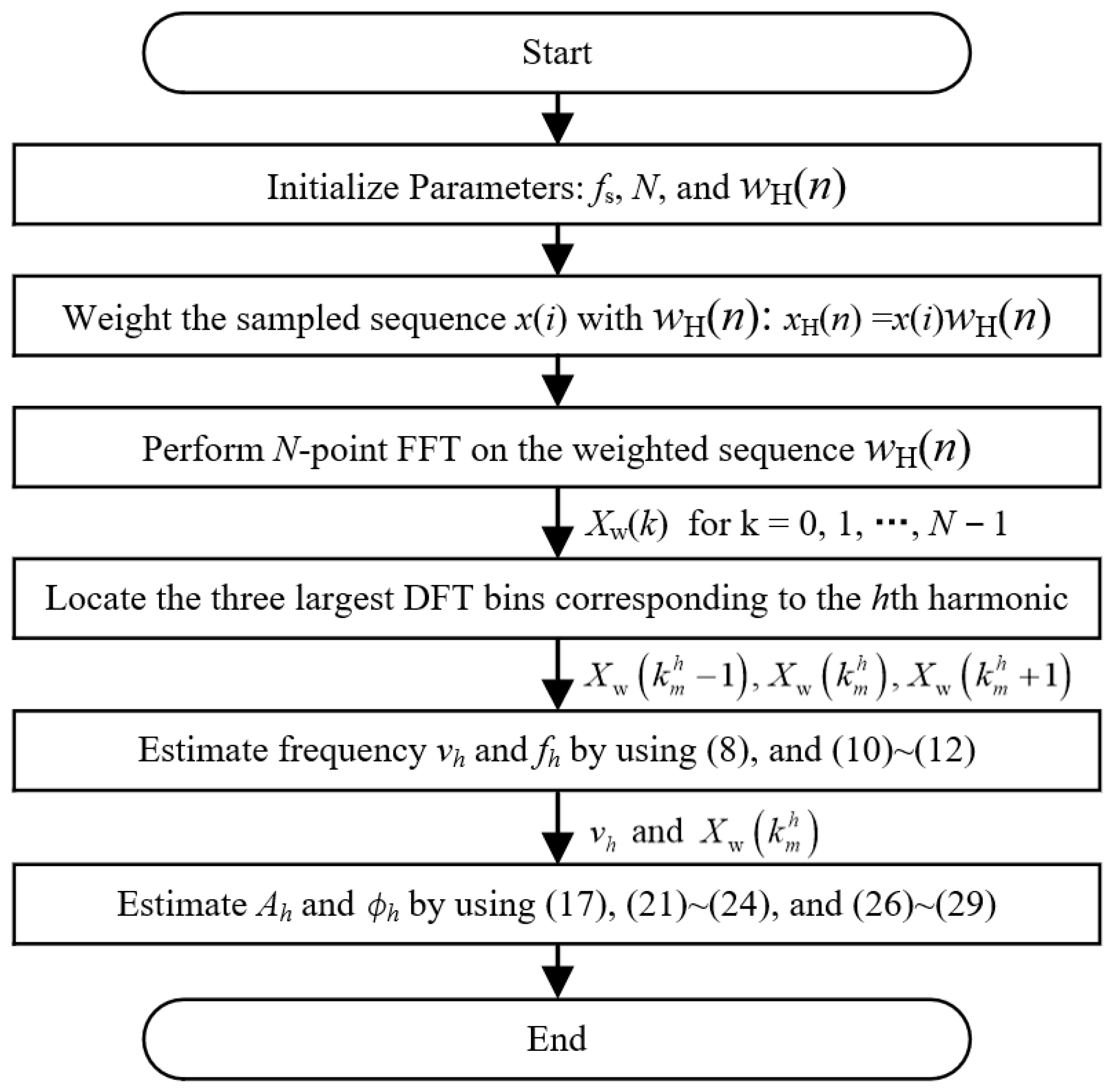
The procedure of the proposed harmonic estimation method is shown in Figure 1. It begins by initializing key parameters, including the sampling frequency f_s, the number of points N, and the weighted sequence corresponding to Hanning window (i.e., w_H(n)). The sampled sequence x(i) is then weighted using N-point Hanning window w_H(n) to produce the windowed sequence x_H(n). An N-point FFT is applied to x_H(n), resulting in the complex spectrum $X_{\mathrm{w}}\left(k\right)$ for k = 0, 1, …, N−1. From this spectrum, the three largest DFT bins—specifically, $X_{\mathrm{w}}\left(k_m^h-1\right)$, $X_{\mathrm{w}}\left(k_m^h\right)$, and $X_{\mathrm{w}}\left(k_m^h+1\right)$—corresponding to the hth harmonic are identified. Using Equations (8) and (10)–(12), the normalized frequency v_h and the actual frequency f_h of the harmonic are accurately estimated. Finally, the amplitude A_h and phase ϕ_h of the harmonic are derived by applying Equations (17), (21)–(24) and (26)–(29), incorporating both $X_{\mathrm{w}}\left(k_m^h\right)$ and the estimated frequency v_h.

3. Simulation Results

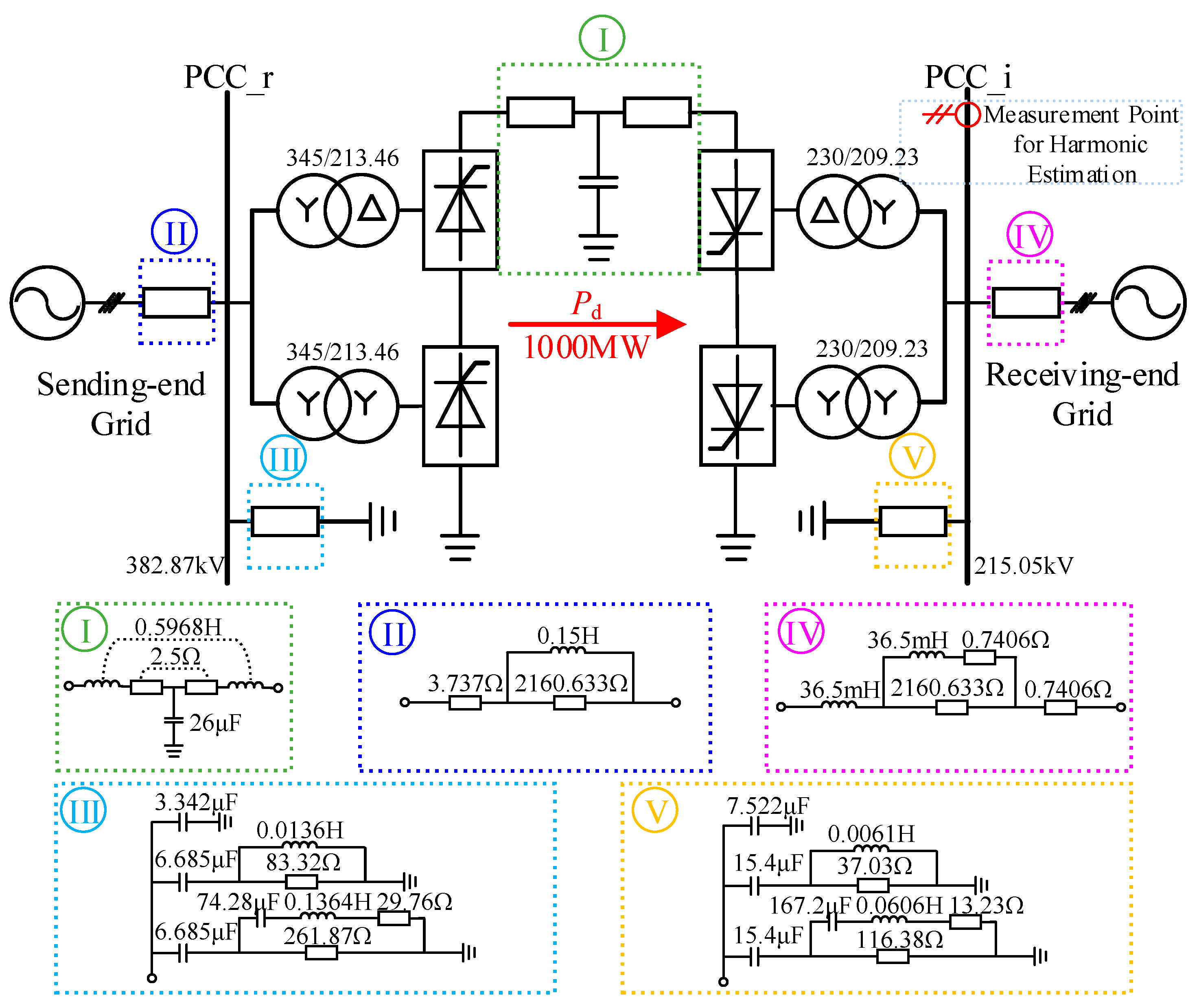
In this section, the Conseil International des Grands Réseaux Électriques (CIGRE) standard model shown in Figure 2 is adopted as the base case. Measurement data collected from the common connection point of the receiving-end system of the LCC-HVDC is used to conduct system simulation tests, with the aim of evaluating the performance of the proposed method. The tests cover frequency deviation interference, noise interference, the effects of sampling frequency and sampling length, a comparative study with state-of-the-art I3pDFT methods, and an evaluation of computational burden. The test signal model for LCC-HVDC system simulations is given in (30), while the signal amplitudes, obtained from the operating system, are provided in

Table 1. Amplitudes of the Harmonic Currents (in Amperes).

h	1	2	3	4	5	6	7
Ah	3968	0.3968	10.317	0.3968	6.7456	0.7936	5.952
h	8	9	10	11	12	13	14
Ah	0.397	4.3648	0.3968	132.13	0	76.582	0
h	15	16	17	18	19	20	21
Ah	0.794	0	0.7936	0	1.984	0	1.984
h	22	23	24	25	26	27	28
Ah	0.397	36.109	0	29.363	0	1.1904	0
h	29	30	31	32	33	34	35
Ah	0.794	0	0.7936	0	0.7936	0	14.682
h	36	37	38	39	-	-	-
Ah	0	14.285	0	1.1904	-	-	-

The bold formatting is used to highlight the harmonic components with relatively large energy proportions in the current waveform of the LCC-HVDC system.

. The estimators were tested using MATLAB R2023b on a computer with 32 GB RAM and a 3.6 GHz processor. In all tests, the phase angle of each frequency component was randomly generated between −π and π for each run. Unless otherwise specified, the fundamental frequency f1 was set to 50.1 Hz, the harmonic frequencies were set as integer multiples of the fundamental frequency, the sampling frequency was 50 kHz, and the sampling length was 10 nominal cycles, corresponding to a total of N = 10,000 samples. For all simulations, the maximum absolute estimation error (MAE) or the mean squared error (MSE) from 2000 independent trials was used as the evaluation metric. Specifically, tests with noise report the MSE, while tests without noise report the MAE. Moreover, since the 12k ± 1 harmonics in LCC-HVDC systems exhibit relatively high magnitudes (as shown in Table 1), the parameter estimation accuracy is reported only for the 11th, 13th, 25th, 27th, 35th, and 37th harmonics in the subsequent experiments.

$$x(t)={\displaystyle \sum _{h=1}^{39}{A}_h}\cos (2\mathsf{\pi }{f}_{1}ht+{\varphi }_h)$$

(30)

3.1. Effect of Frequency Deviation

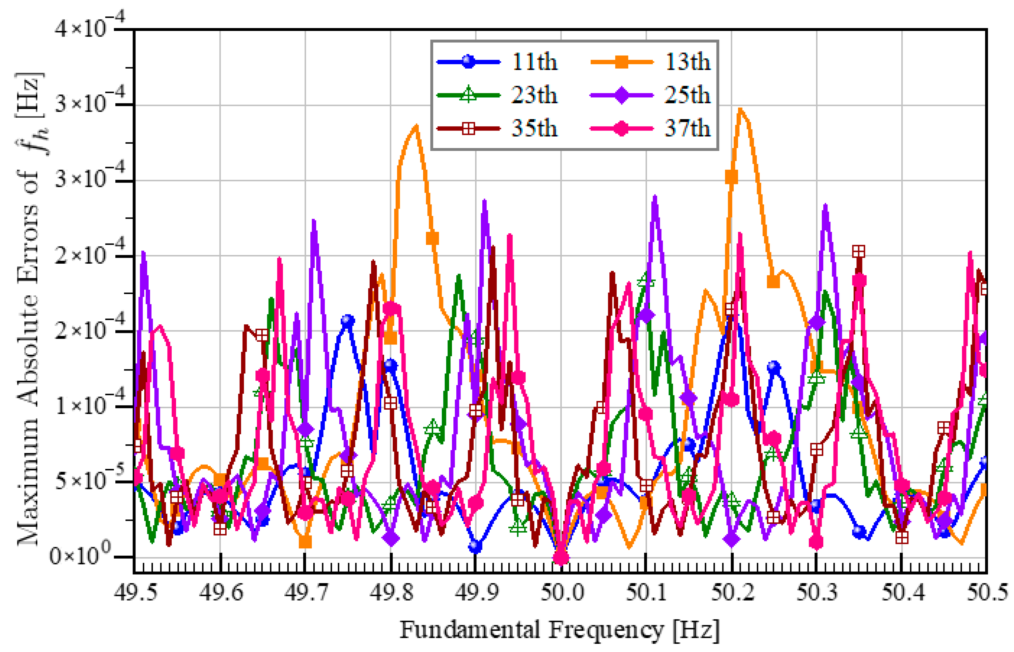
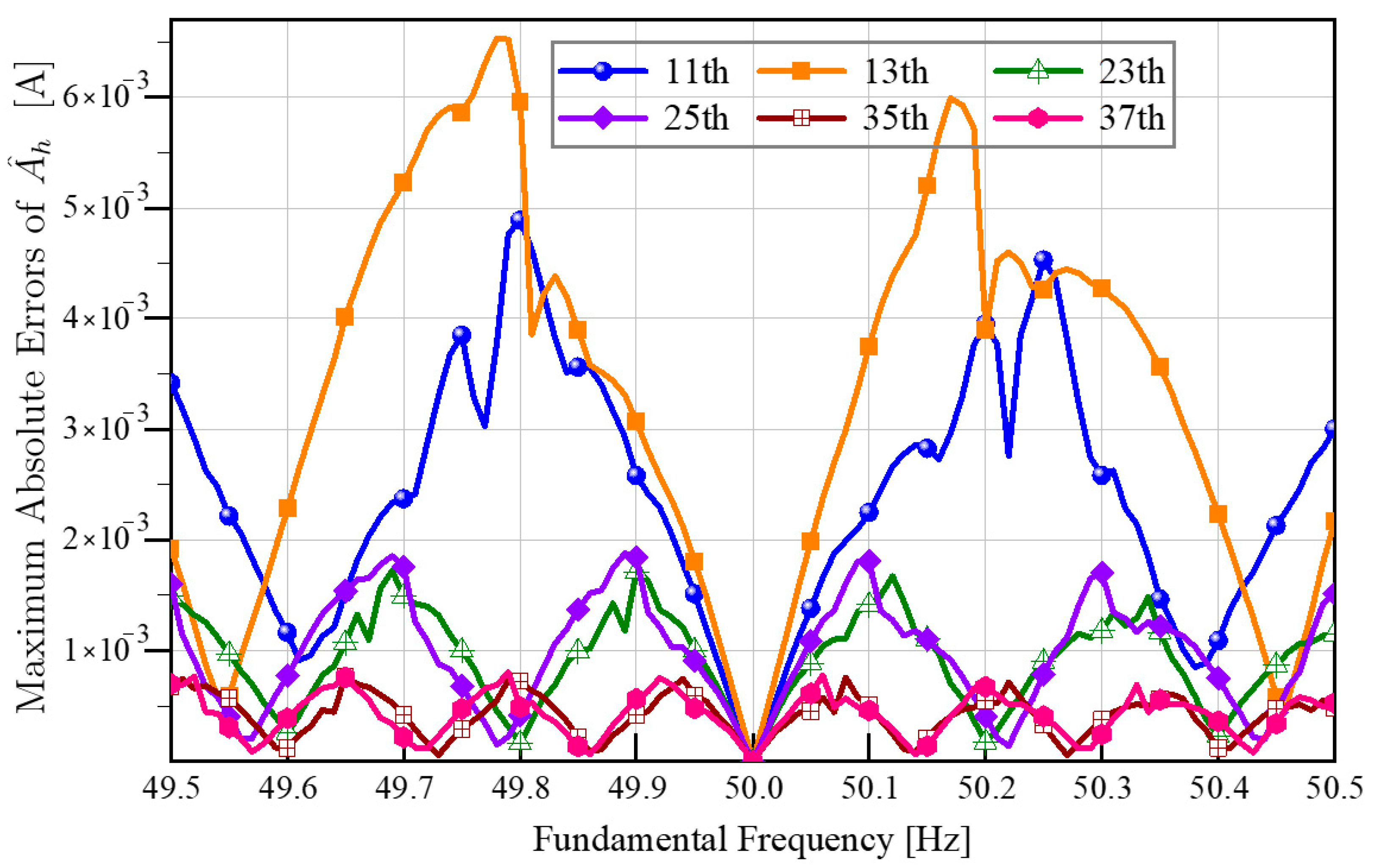
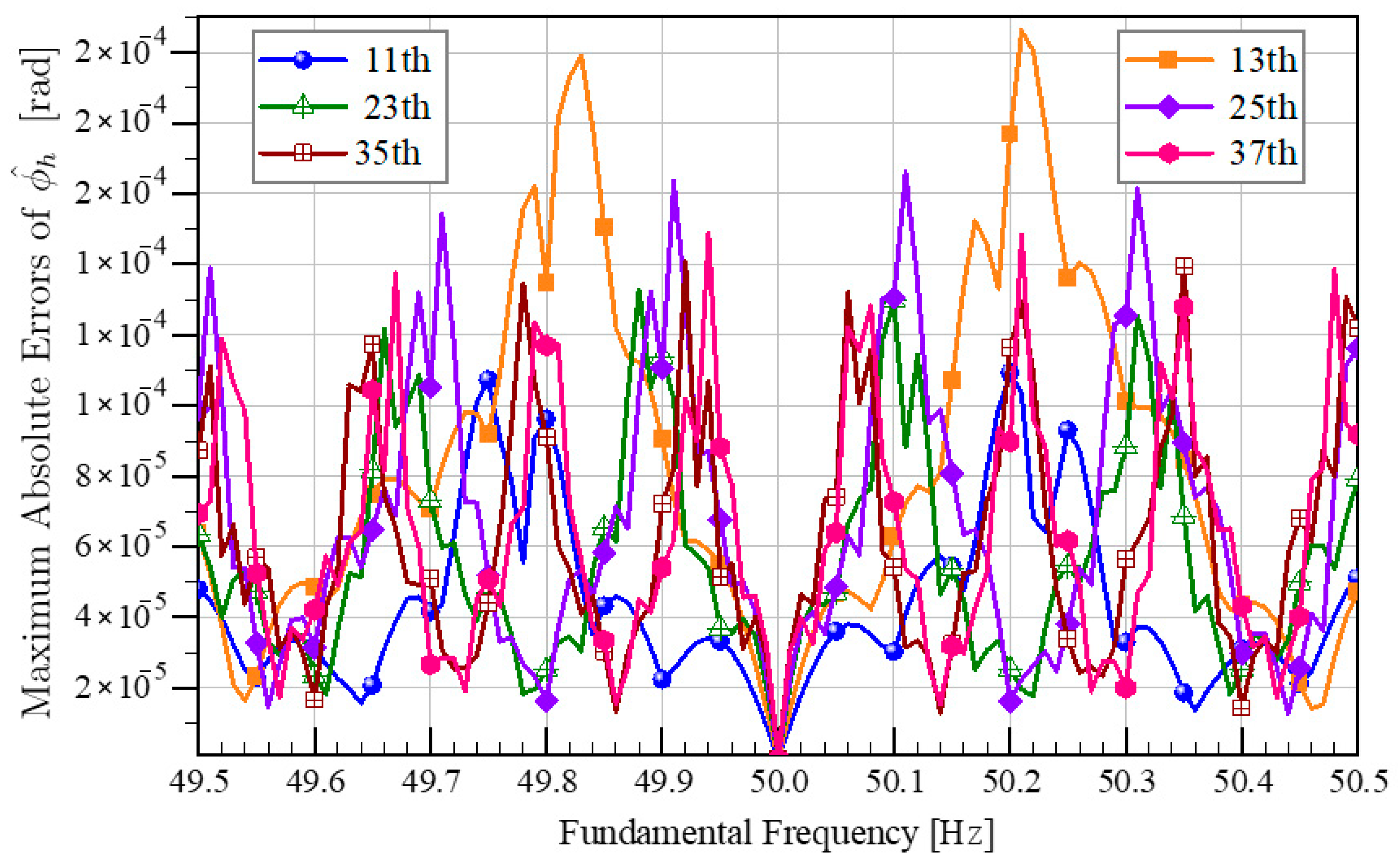
The frequency of an actual system typically fluctuates around its nominal value. For a system with a nominal frequency of 50 Hz, relevant standards specify that the frequency deviation must not exceed ±0.5 Hz. Therefore, in this test, the frequency was varied from 49.5 Hz to 50.5 Hz in steps of 0.01 Hz. At each frequency point, the MAEs of frequency, amplitude, and phase angle were obtained from 2000 independent experiments and are reported. The MAEs of the proposed method for harmonic frequency, amplitude, and phase angle under frequency deviation conditions are presented in Figure 3, Figure 4 and Figure 5.

As shown in Figure 3, when the fundamental frequency fluctuates within the range of 49.5–50.5 Hz, the proposed method achieves relatively low MAEs in frequency estimating the 11th, 13th, 23rd, 25th, 35th, and 37th harmonics. The overall error level remains within 10⁻⁵~10⁻⁴ Hz, with only minor variations as the fundamental frequency changes. Specifically, the maximum estimation errors occur at different frequencies for different harmonic orders, and the error distribution exhibits approximate symmetry around 50 Hz. Among them, the 13th harmonic shows the largest estimation errors, reaching 0.286 mHz and 0.298 mHz at 49.83 Hz and 50.21 Hz, respectively. Figure 4 shows that the amplitude estimation errors of all harmonics under frequency deviation interference remain below 6.6 × 10⁻³ A. The 23rd, 25th, 35th, and 37th harmonics exhibit relatively small errors, all within 2 × 10⁻³ A. In contrast, the 11th and 13th harmonics show comparatively larger errors, reaching maximum values of 4.886 × 10⁻³ A at 49.8 Hz and 6.533 × 10⁻³ A at 49.78 Hz, respectively. As illustrated in Figure 5, the MAEs of the phase estimation for each harmonic component show a trend similar to the frequency estimation results. Specifically, the 13th harmonic exhibits the highest MAEs, which occur at fundamental frequencies of 49.83 Hz and 50.21 Hz, with corresponding values of 1.990 × 10⁻⁴ A and 2.062 × 10⁻⁴ A, respectively. Overall, the results demonstrate that the proposed method achieves robust and stable performance under frequency deviation.

3.2. Effect of Noise Interference

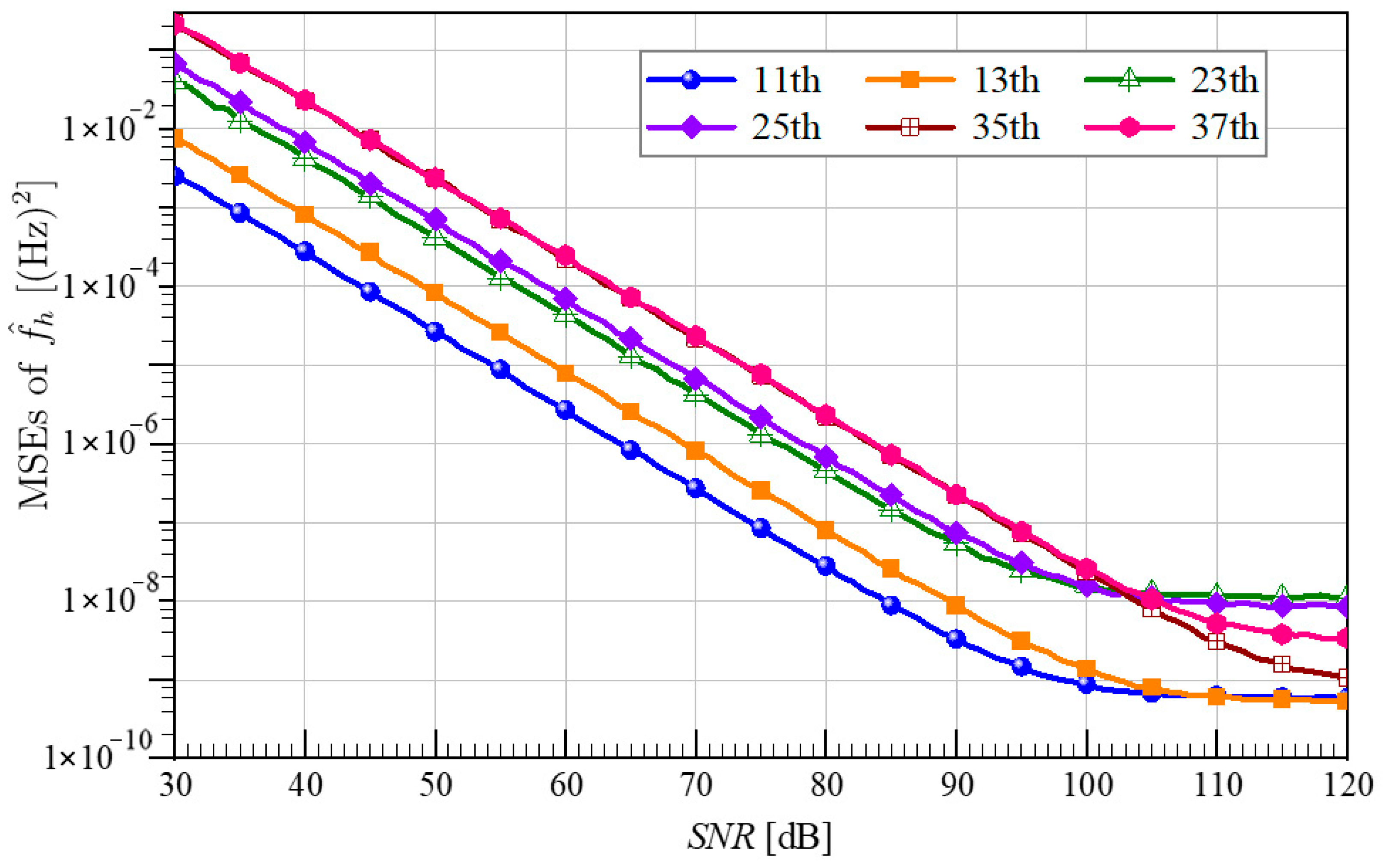
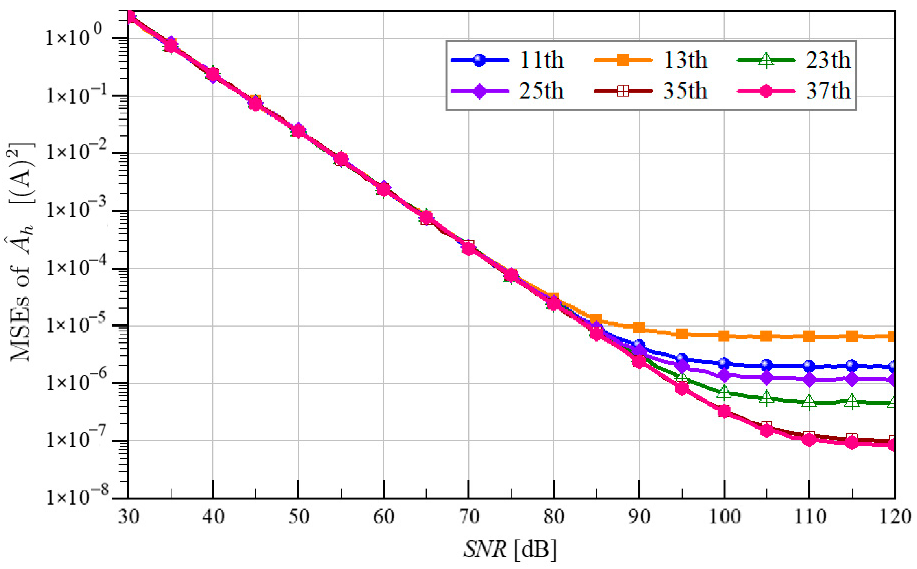
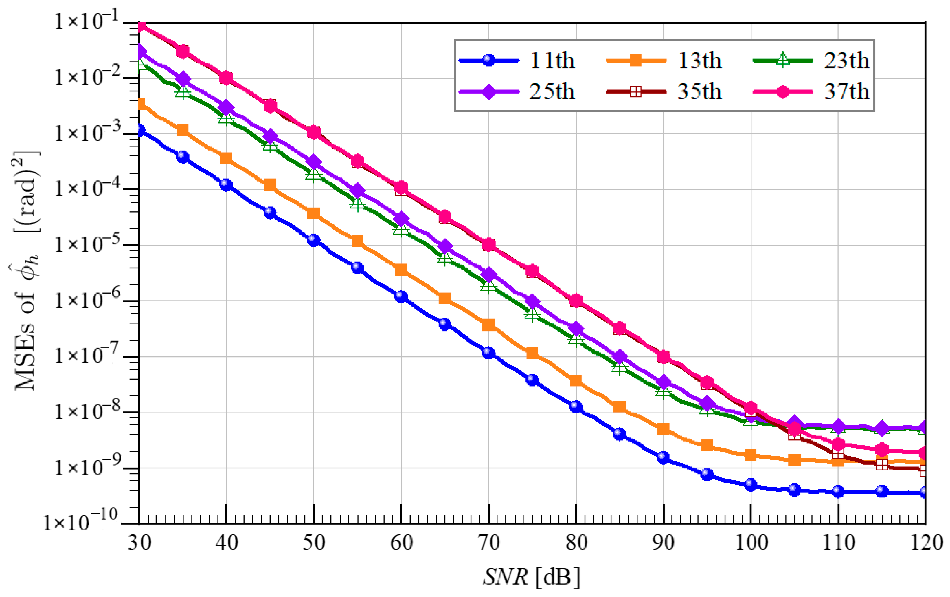
Noise is unavoidable in practical measurements. In this subsection, the performance of the proposed method is evaluated through simulations under different Signal-to-Noise Ratios (SNRs). For the noise interference test, the SNR was varied from 30 dB to 120 dB in steps of 1 dB. In each independent run, the phase angles of the harmonics were initialized independently and randomly following a uniform distribution over [−π, π]. At a given SNR, the MSE was computed from an ensemble of 2000 Monte Carlo simulations and is reported in Figure 6, Figure 7 and Figure 8.

The harmonic frequency estimation performance is illustrated in Figure 6. The estimation error of the harmonic frequency increases as the harmonic order rises. This occurs because, when additive white Gaussian noise is introduced into the signal, the SNR is calculated with respect to the fundamental component, while the amplitudes of higher-order harmonics decrease with increasing order. Consequently, at a fixed SNR, higher-order harmonics exhibit larger estimation errors. Furthermore, when the SNR is below 90 dB, the estimation error is primarily dominated by noise interference, and the MSEs of the harmonic frequency estimates decrease approximately linearly with increasing SNR. However, once the SNR exceeds 90 dB, the estimation variance of the harmonic frequencies no longer decreases significantly, as the dominant error source shifts from noise to interference between adjacent harmonics.

The performance of harmonic amplitude estimation is illustrated in Figure 7. When the SNR ranges from 30 dB to 80 dB, the MSE of the amplitude estimates decreases approximately linearly with increasing SNR. Notably, the estimation performance remains nearly consistent across different harmonics and is largely independent of their actual amplitudes. Once the SNR exceeds 80 dB, spectral leakage gradually becomes the dominant source of error, and further improvements in SNR no longer enhance estimation accuracy. At sufficiently high SNR levels, where noise has negligible influence, the accuracy of harmonic amplitude estimation depends mainly on the harmonic position in frequency domain. The performance of harmonic phase angle estimation is presented in Figure 8, exhibiting a similar trend to that of harmonic frequency estimation and thus is not discussed in detail here.

3.3. Effect of Variable Sampling Rates

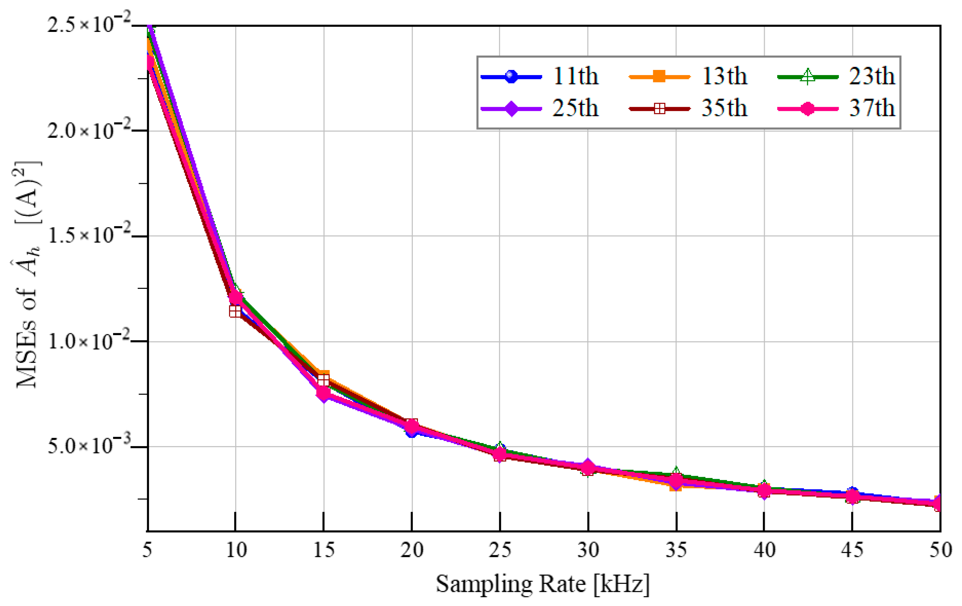
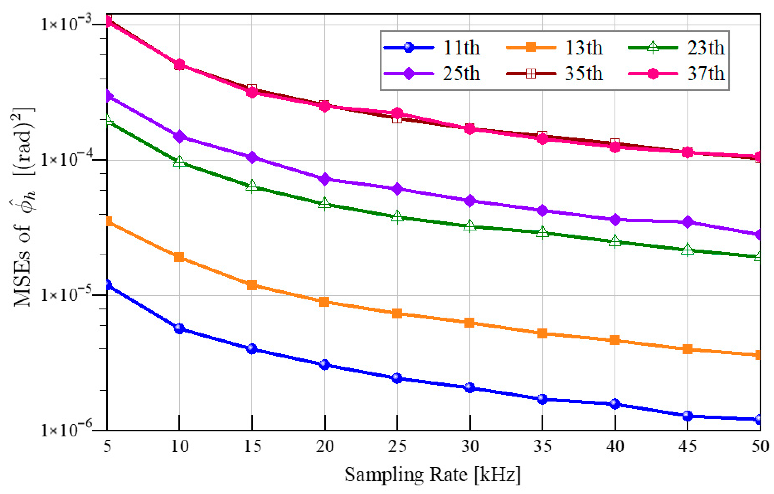
In this subsection, simulations are performed to evaluate the impact of sampling frequency on the estimation accuracy of the proposed method. The sampling frequency is varied from 5 kHz to 50 kHz in increments of 5 kHz, while the sampling window length is fixed at 10 nominal cycles. Accordingly, the number of sampling points N ranges from 1000 to 10,000 in steps of 1000 points. To clearly demonstrate the influence of sampling frequency, both noiseless signals and signals corrupted by 60 dB additive noise are considered. For the noiseless case, the MAE is adopted to assess the estimation accuracy of odd-harmonic frequencies, amplitudes, and phase angles. For the noisy case with 60 dB SNR, the MSE is used to evaluate the accuracy of the same harmonic parameters.

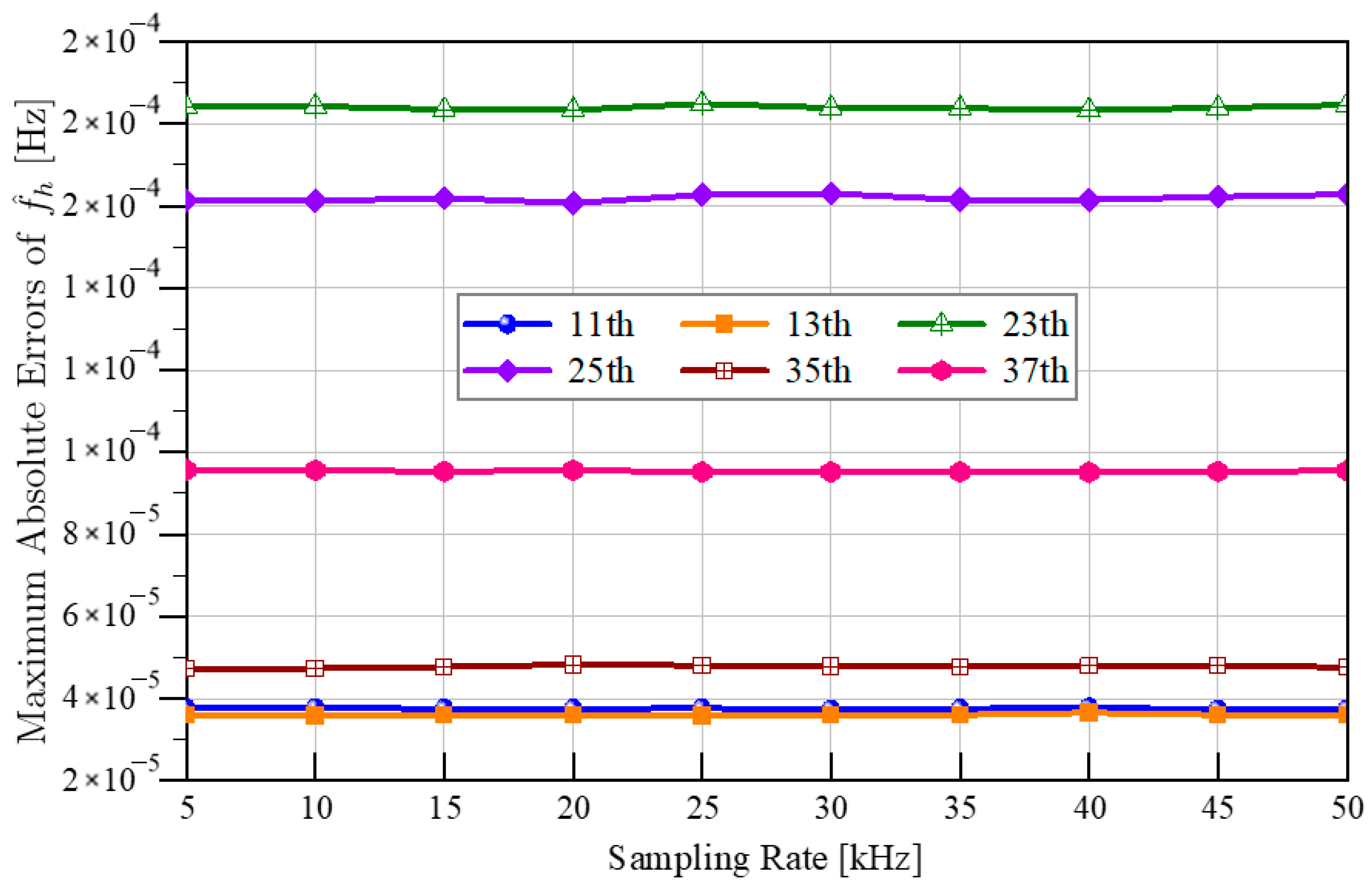
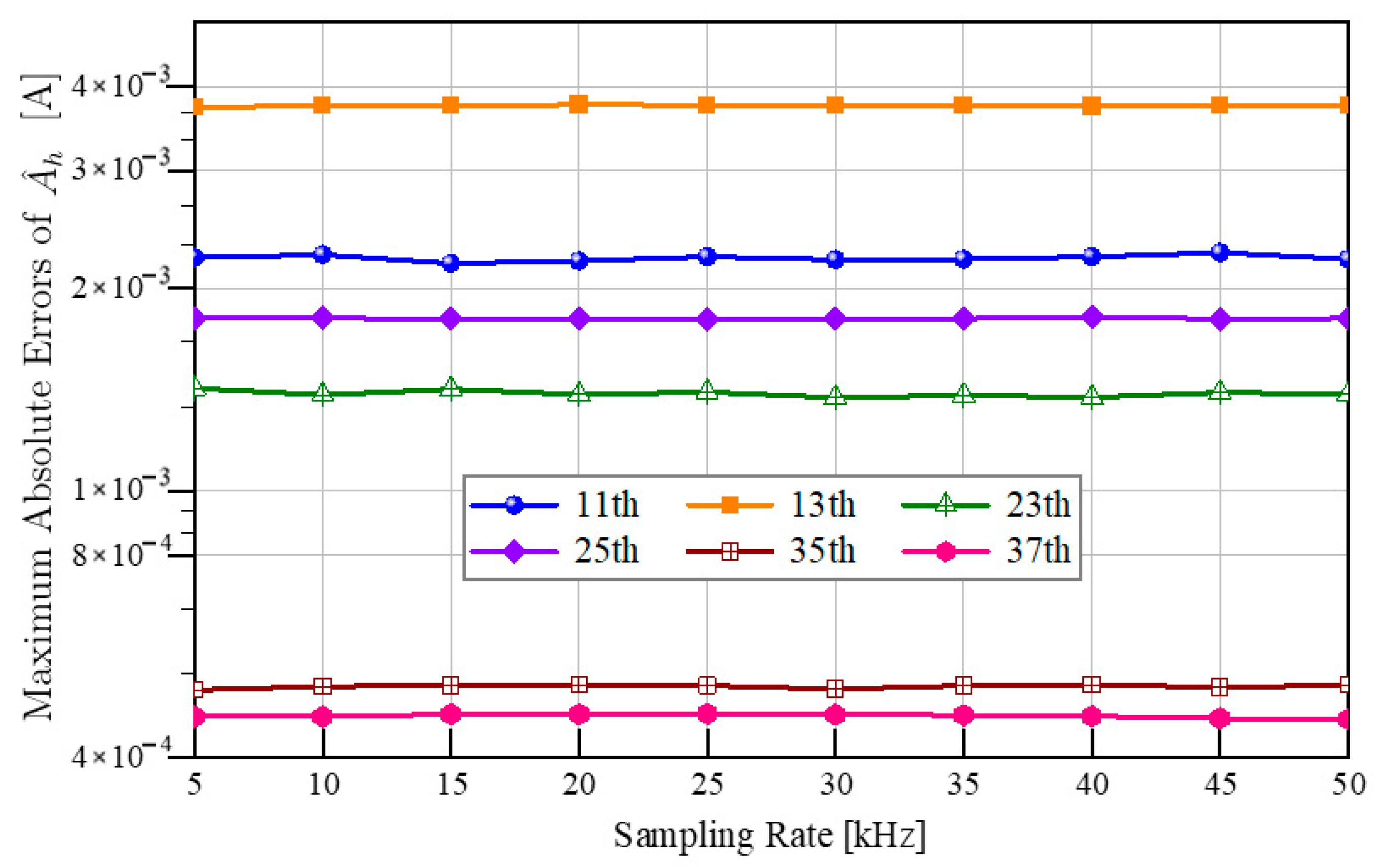
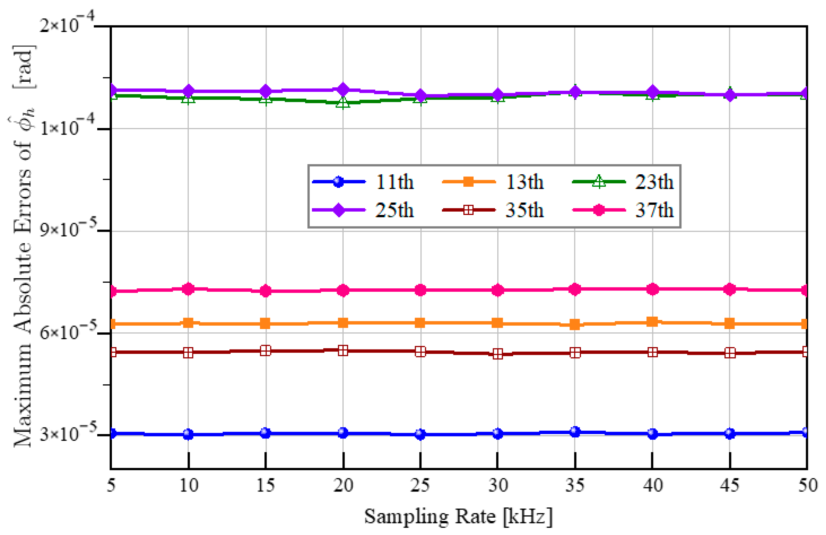
Under noise-free conditions, the estimation errors of harmonic frequency, amplitude, and phase angle using the proposed method at different sampling frequencies are shown in Figure 9, Figure 10, and Figure 11, respectively. It can be observed that, when the sampling window length is kept constant, increasing the sampling frequency does not improve the estimation accuracy of harmonic parameters. This is because, with a fixed sampling window length, the frequency resolution of the DFT spectrum is also fixed; in the absence of other interference sources, the estimation error of the proposed method remains constant. Specifically, the maximum absolute estimation errors of the harmonic frequency, amplitude, and phase angle do not exceed 0.2 mHz, 4 mA, and 0.0002 rad, respectively.

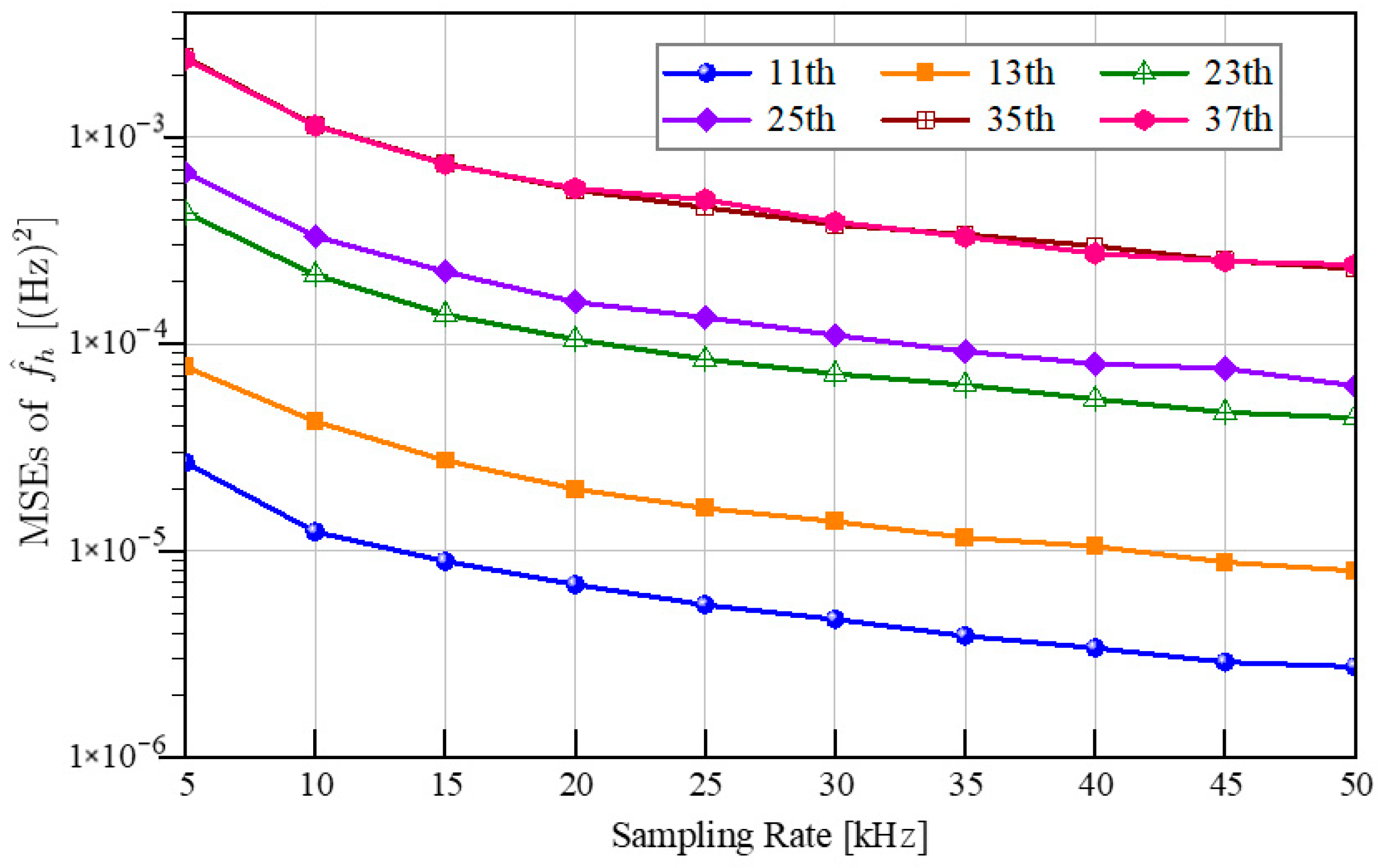
Under 60 dB noise conditions, the estimation errors of harmonic frequency, amplitude, and phase angle using the proposed method at different sampling frequencies are shown in Figure 12, Figure 13 and Figure 14, respectively. It can be observed that, when the sampling window length is kept constant, the estimation accuracy of harmonic parameters improves as the sampling frequency increases. This behavior differs from the noise-free case because, with a fixed window length, the number of sampling points increases with the sampling frequency, thereby enhancing the noise robustness of the proposed method. However, this improvement comes at the cost of reduced computational efficiency. Therefore, in practical applications, an appropriate sampling frequency can be chosen according to the desired trade-off between noise robustness and computational efficiency. Moreover, under noise interference, the estimation performance of harmonic frequency and phase deteriorates as the harmonic order increases (Figure 12 and Figure 14). This is due to the decreasing amplitudes of higher-order harmonics. In contrast, Figure 12 shows that the proposed method’s performance in estimating harmonic amplitudes is minimally affected by the harmonic amplitude itself.

3.4. Effect of Sampling Window Length

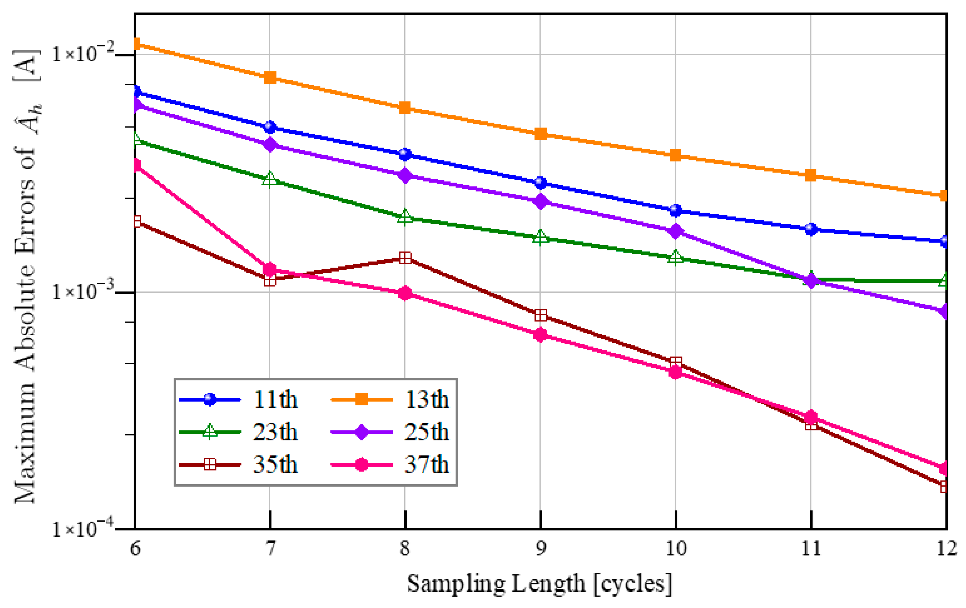
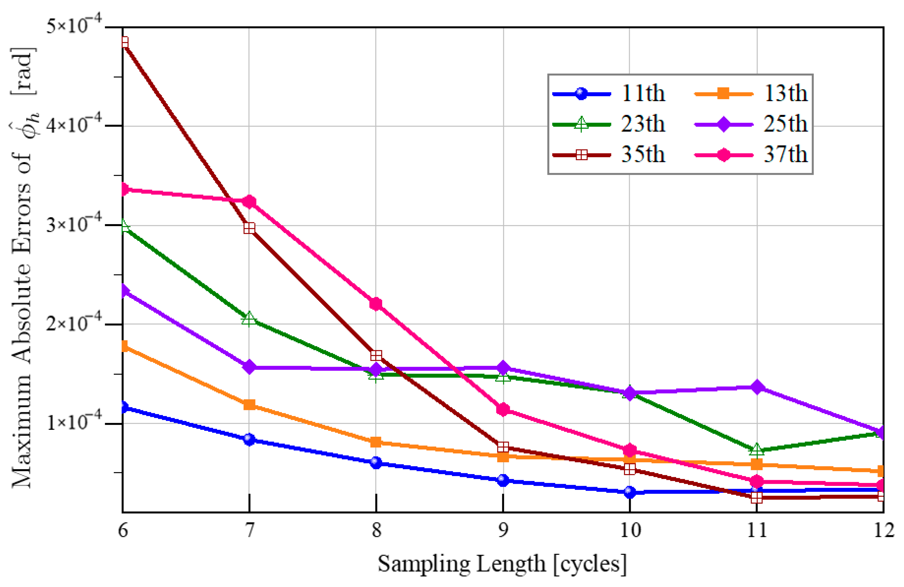
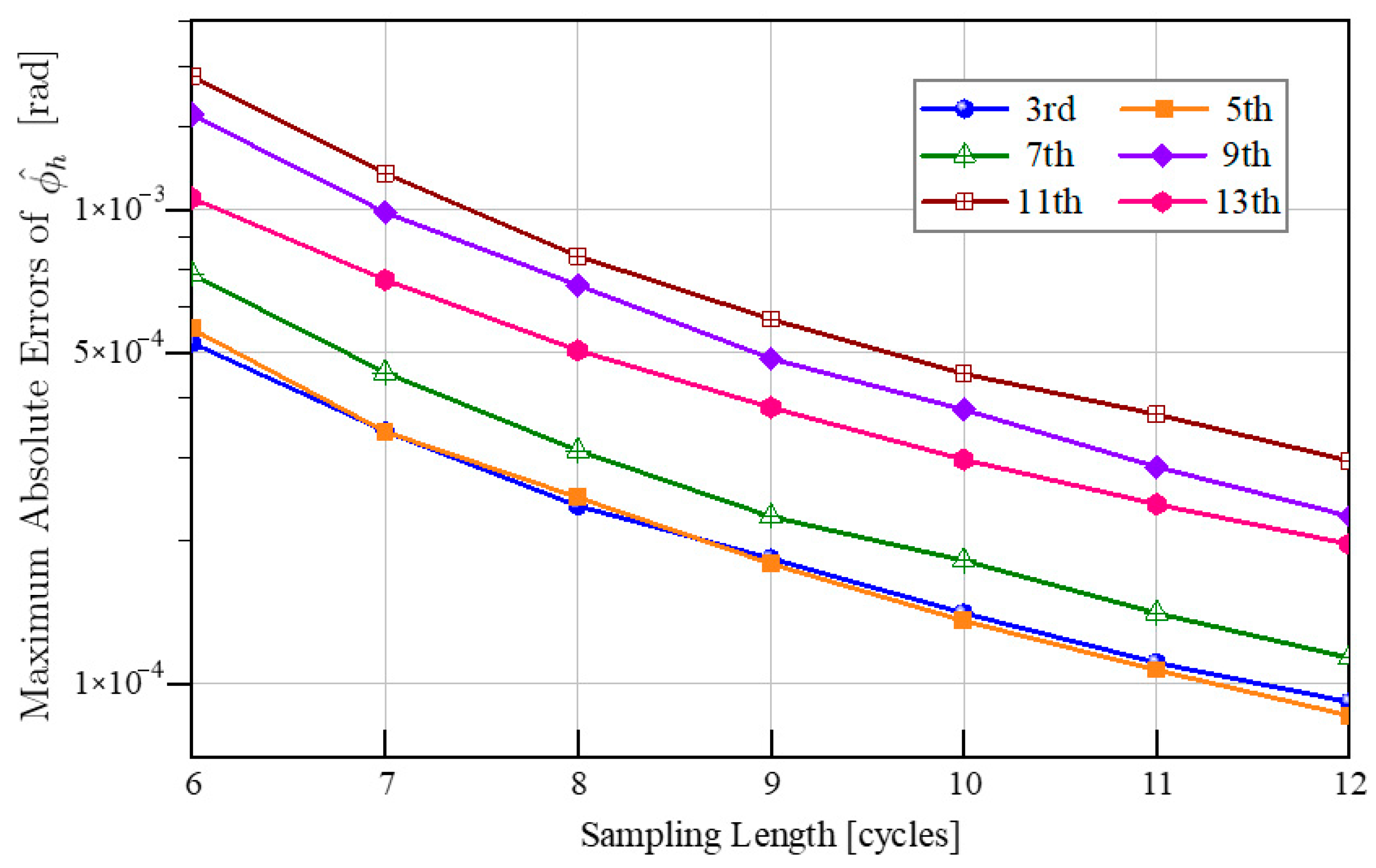
In this subsection, simulations are performed to evaluate the impact of sampling length on the estimation accuracy of the proposed method. The sampling length is varied from 6 cycles to 12 cycles in increments of 1 cycle, while the sampling rate is fixed at 50 kHz. Accordingly, the number of sampling points N ranges from 6000 to 12,000 in steps of 1000 points. The results are presented in Figure 15, Figure 16 and Figure 17.

As shown in Figure 15, Figure 16 and Figure 17, as the sampling length increases from 6 to 12 cycles, the MAEs of harmonic frequency, amplitude, and phase angle decrease accordingly, indicating that the estimation accuracy of harmonic parameters improves with longer sampling windows. This is because, with a fixed sampling rate, increasing the sampling length essentially enhances the frequency resolution of the DFT spectrum. The improved frequency resolution reduces the effects of the spectral leakage between harmonics, thereby improving the estimation accuracy of the proposed method. However, a longer sampling length also results in a longer measurement response time, which is unfavorable for real-time harmonic parameter measurement. Therefore, in practical applications, the sampling length can be adjusted to achieve a balance between estimation accuracy and response speed. From the estimation performance of each harmonic, the estimation errors for magnitude and phase exhibit an inverse trend. Overall, higher-order harmonics correspond to smaller magnitude errors but increasingly larger phase errors.

3.5. Comparison with Other Methods

To evaluate the performance of the proposed harmonic parameter estimation method based on I3pDFT with a Hanning window, two classical or advanced peer methods, namely Method 1 [47] and Method 2 [44], are selected for comparison. Both the comparative algorithms and the proposed method employ the Hanning window to suppress spectral leakage and estimate harmonic parameters from the three largest DFT spectral lines. However, their estimation formulas for frequency, amplitude, and phase differ from those of the proposed method, which constitutes the key distinction of this work from other DFT-based approaches. In the test, the fundamental frequency is set to 50.1 Hz, the sampling frequency to 50 kHz, and the sampling lengths to 6 and 10 nominal cycles, respectively. Two conditions are considered: noise-free and with 60 dB noise interference.

The test results for the noise-free signal are presented in

Table 2. Harmonic Estimation Results of Different Methods under Noise-Free Condition with 6 Cycles.

Harmonic Order	MAEs of Frequency (mHz)			MAEs of Amplitude (V)			MAEs of Phase Angle (Rad)
	Proposed	Method 1	Method 2	Proposed	Method 1	Method 2	Proposed	Method 1	Method 2
11	1.241 × 10−5	1.267 × 10−5	1.260 × 10−5	4.132 × 10−3	4.114 × 10−3	4.119 × 10−3	2.061 × 10−6	2.096 × 10−6	2.087 × 10−6
13	3.612 × 10−5	3.741 × 10−5	3.718 × 10−5	4.141 × 10−3	4.120 × 10−3	4.123 × 10−3	5.808 × 10−6	5.989 × 10−6	5.957 × 10−6
23	1.730 × 10−4	1.906 × 10−4	1.895 × 10−4	3.933 × 10−3	3.863 × 10−3	3.866 × 10−3	2.781 × 10−5	3.033 × 10−5	3.018 × 10−5
25	2.453 × 10−4	2.757 × 10−4	2.741 × 10−4	3.703 × 10−3	3.635 × 10−3	3.638 × 10−3	3.995 × 10−5	4.435 × 10−5	4.412 × 10−5
35	1.087 × 10−3	1.341 × 10−3	1.336 × 10−3	3.966 × 10−3	3.907 × 10−3	3.909 × 10−3	1.793 × 10−4	2.157 × 10−4	2.149 × 10−4
37	1.321 × 10−3	1.657 × 10−3	1.648 × 10−3	3.872 × 10−3	3.827 × 10−3	3.827 × 10−3	2.201 × 10−4	2.676 × 10−4	2.665 × 10−4

The bold formatting is used to indicate the minimum error obtained by the three methods.

and

Table 3. Harmonic Estimation Results of Different Methods under Noise-Free Condition with 10 Cycles.

Harmonic Order	MAEs of Frequency (mHz)			MAEs of Amplitude (V)			MAEs of Phase Angle (Rad)
	Proposed	Method 1	Method 2	Proposed	Method 1	Method 2	Proposed	Method 1	Method 2
11	2.641 × 10−6	2.841 × 10−6	2.823 × 10−6	2.368 × 10−3	2.339 × 10−3	2.341 × 10−3	1.197 × 10−6	1.279 × 10−6	1.272 × 10−6
13	7.959 × 10−6	8.695 × 10−6	8.647 × 10−6	2.466 × 10−3	2.423 × 10−3	2.426 × 10−3	3.573 × 10−6	3.869 × 10−6	3.849 × 10−6
23	4.395 × 10−5	5.668 × 10−5	5.641 × 10−5	2.446 × 10−3	2.392 × 10−3	2.392 × 10−3	1.915 × 10−5	2.398 × 10−5	2.388 × 10−5
25	6.945 × 10−5	9.277 × 10−5	9.183 × 10−5	2.479 × 10−3	2.536 × 10−3	2.526 × 10−3	3.161 × 10−5	4.073 × 10−5	4.043 × 10−5
35	2.226 × 10−4	2.527 × 10−4	2.533 × 10−4	2.343 × 10−3	2.299 × 10−3	2.298 × 10−3	1.005 × 10−4	1.127 × 10−4	1.129 × 10−4
37	2.285 × 10−4	2.494 × 10−4	2.500 × 10−4	2.360 × 10−3	2.326 × 10−3	2.325 × 10−3	1.034 × 10−4	1.114 × 10−4	1.117 × 10−4

The bold formatting is used to indicate the minimum error obtained by the three methods.

. With a sampling length of 6 nominal cycles, the proposed method yields smaller maximum amplitude estimation errors than the two reference methods. In terms of frequency and phase estimation, it achieves smaller errors for the 13th, 25th, and 37th harmonics. Although it does not outperform the others for the 11th, 23rd, and 35th harmonics, the differences among the three methods are negligible. When the sampling length is increased to 10 nominal cycles, the proposed method also attains smaller maximum amplitude estimation errors. While it does not exhibit the smallest errors in frequency and phase estimation, the differences among the three methods remain minimal. Moreover, the maximum absolute estimation error of the proposed method is consistently below 1 mHz, 0.02 A, and 0.001 rad. Compared with the 6-cycle sampling, the estimation errors are significantly reduced with 10-cycle sampling, as the longer sampling length improves frequency resolution, alleviates spectral leakage between adjacent harmonics, and enhances the accuracy of harmonic parameter estimation.

The test results for the 60 dB noise signals are presented in

Table 4. Harmonic Estimation Results of Different Methods under 50 dB Noise with 6 Cycles.

Harmonic Order	MSEs of Frequency [(Hz/Hz)2]			MSEs of Amplitude [V2]			MAEs of Phase Angle [Rad2]
	Proposed	Method 1	Method 2	Proposed	Method 1	Method 2	Proposed	Method 1	Method 2
11	1.241 × 10−5	1.267 × 10−5	1.260 × 10−5	4.132 × 10−3	4.114 × 10−3	4.119 × 10−3	2.061 × 10−6	2.096 × 10−6	2.087 × 10−6
13	3.612 × 10−5	3.741 × 10−5	3.718 × 10−5	4.141 × 10−3	4.120 × 10−3	4.123 × 10−3	5.808 × 10−6	5.989 × 10−6	5.957 × 10−6
23	1.730 × 10−4	1.906 × 10−4	1.895 × 10−4	3.933 × 10−3	3.863 × 10−3	3.866 × 10−3	2.781 × 10−5	3.033 × 10−5	3.018 × 10−5
25	2.453 × 10−4	2.757 × 10−4	2.741 × 10−4	3.703 × 10−3	3.635 × 10−3	3.638 × 10−3	3.995 × 10−5	4.435 × 10−5	4.412 × 10−5
35	1.087 × 10−3	1.341 × 10−3	1.336 × 10−3	3.966 × 10−3	3.907 × 10−3	3.909 × 10−3	1.793 × 10−4	2.157 × 10−4	2.149 × 10−4
37	1.321 × 10−3	1.657 × 10−3	1.648 × 10−3	3.872 × 10−3	3.827 × 10−3	3.827 × 10−3	2.201 × 10−4	2.676 × 10−4	2.665 × 10−4

The bold formatting is used to indicate the minimum error obtained by the three methods.

and

Table 5. Harmonic Estimation Results of Different Methods under 50 dB Noise with 10 Cycles.

Harmonic Order	MSE of Amplitude			MSE of Frequency			MSE of Phase
	Proposed	Method 1	Method 2	Proposed	Method 1	Method 2	Proposed	Method 1	Method 2
11	2.641 × 10−6	2.841 × 10−6	2.823 × 10−6	2.368 × 10−3	2.339 × 10−3	2.341 × 10−3	1.197 × 10−6	1.279 × 10−6	1.272 × 10−6
13	7.959 × 10−6	8.695 × 10−6	8.647 × 10−6	2.466 × 10−3	2.423 × 10−3	2.426 × 10−3	3.573 × 10−6	3.869 × 10−6	3.849 × 10−6
23	4.395 × 10−5	5.668 × 10−5	5.641 × 10−5	2.446 × 10−3	2.392 × 10−3	2.392 × 10−3	1.915 × 10−5	2.398 × 10−5	2.388 × 10−5
25	6.945 × 10−5	9.277 × 10−5	9.183 × 10−5	2.479 × 10−3	2.536 × 10−3	2.526 × 10−3	3.161 × 10−5	4.073 × 10−5	4.043 × 10−5
35	2.226 × 10−4	2.527 × 10−4	2.533 × 10−4	2.343 × 10−3	2.299 × 10−3	2.298 × 10−3	1.005 × 10−4	1.127 × 10−4	1.129 × 10−4
37	2.285 × 10−4	2.494 × 10−4	2.500 × 10−4	2.360 × 10−3	2.326 × 10−3	2.325 × 10−3	1.034 × 10−4	1.114 × 10−4	1.117 × 10−4

The bold formatting is used to indicate the minimum error obtained by the three methods.

. With a sampling length of 6 nominal cycles, the proposed method achieves lower MSEs in frequency and phase angle estimation for all considered harmonics compared with the two reference methods. Although its amplitude estimation MSEs are not superior to those of the reference methods, the differences are negligible. When the sampling length is increased to 10 nominal cycles, the performance trend between the proposed and reference methods remains similar to that observed with 6 cycles, while all MSEs are significantly reduced. This improvement is attributed to the larger number of sampling points provided by the longer sampling length, which enhances the noise immunity of the proposed method. Overall, compared with the reference methods, the proposed method demonstrates superior performance in harmonic frequency and phase angle estimation under noisy conditions. Regarding amplitude estimation, the error differences relative to the reference methods are minimal and can be practically neglected. These results confirm that the novel combination of frequency, amplitude, and phase estimation formulas employed in the proposed method provides distinct advantages in harmonic frequency and phase angle estimation.

3.6. Analysis of Computational Burden

In this subsection, the computational efficiency of the proposed method is evaluated. The simulations were conducted using MATLAB R2024a on a hardware platform consisting of a laptop computer equipped with a 2.3 GHz processor and 16 GB of RAM. The sampling frequency in this test was set to 50 kHz, and the sampling lengths corresponding to 6, 8, 10, and 12 nominal cycles were considered. Each scenario was executed 2000 times, and the average time per run was reported. To visually demonstrate the computational efficiency of the proposed method, two of the most advanced or classical I3pDFT methods (namely, Method 1 [47] and Method 2 [44]) were selected as references for comparison.

The test results for the computational overhead of the proposed method are shown in

Table 6. Average Runtime per Execution of Different Methods.

Methods	6 Cycles	8 Cycles	10 Cycles	12 Cycles
Method 1	0.666 ms	0.753 ms	0.792 ms	0.841 ms
Method 2	0.604 ms	0.677 ms	0.701ms	0.762 ms
Proposed	0.791 ms	0.854 ms	0.928 ms	0.988 ms

. Although the computational overhead of the proposed method is higher than that of the other two methods, its absolute computational cost remains small. Taking 12 nominal cycles (i.e., 12,000 sampling points) as an example, the average execution time of the proposed algorithm remains below 1 ms. In fact, the computational load of all three methods primarily comes from two parts: first, the execution of the FFT procedure, which constitutes the major portion of the computational overhead, and second, the subsequent frequency, amplitude, and phase calculations, which account for a relatively small share of the total computational cost. Differences in the formulae used by each method lead to variations in computational expense. Therefore, although the computational load of the parameter estimation formulae in the proposed method is slightly higher than that of the other two I3pDFT-based harmonic parameter estimation methods, it remains a suitable candidate for resource-constrained embedded platforms.

In LCC-HVDC systems, the characteristic harmonics are predominantly of the order 12k ± 1 (k = 1, 2, …), which correspond to the 11th, 13th, 25th, 27th, 35th, and 37th harmonics. These harmonics exhibit relatively high magnitudes and their adverse effects on the power system are well recognized. Specifically, the 11th and 13th harmonics can cause significant distortion in the voltage and current waveforms at the converter bus, increasing the stress on converter valves and leading to additional losses in transformers and filters. The 25th and 27th harmonics, although smaller in amplitude, may interact with the AC network resonance points and cause amplification of harmonic distortion, potentially affecting the stability of nearby protection devices. The 35th and 37th harmonics, being of higher frequency, are more susceptible to propagation through the AC filters and can introduce high-frequency oscillations, which may interfere with control and communication equipment. Therefore, accurate estimation of these harmonics is not only essential for harmonic mitigation but also crucial for assessing the overall system reliability and equipment lifetime. The simulation results in this paper demonstrate that the proposed method achieves high estimation accuracy for these critical harmonics under various operating conditions, thereby providing a reliable basis for subsequent harmonic control and filter design.

4. Conclusions

This paper presented a novel three-point interpolated DFT method based on the Hanning window (I3pDFT) for harmonic parameter estimation in LCC-HVDC systems. By leveraging the balanced characteristics of the Hanning window and an improved interpolation formula, the proposed method effectively suppresses spectral leakage and achieves high-precision estimation of the harmonic frequency, amplitude, and phase angle. Simulation results under diverse conditions—including frequency deviation, noise interference, varying sampling rates, and different observation lengths—validated its superior performance compared to two widely used I3pDFT algorithms. In particular, the method consistently reduced estimation errors of higher-order harmonics and showed strong robustness against noise, even at low SNR levels. Although the computational cost of the proposed algorithm is slightly higher than that of reference methods, the runtime remains below 1 ms for practical sampling lengths, ensuring feasibility for real-time and embedded applications. Overall, the proposed I3pDFT-Hanning method offers clear advantages in accuracy, robustness, and practical applicability. Future work may extend this framework by optimizing window selection and interpolation strategies for non-stationary signals, further enhancing its adaptability to complex power quality environments. The findings highlight the method’s potential as a reliable tool for next-generation harmonic measurement and wideband impedance monitoring in LCC-HVDC systems.

References

1. Zhang, J.; Hu, X.; Zhang, C.; Song, J.; Shi, G.; Xu, X.; Wen, H. High Precision Parameter Estimator for Calibrating the Sine Wave Signals in Industrial Inspection. IEEE Trans. Ind. Inform. 2025. [Google Scholar] [CrossRef]
2. Zhang, J.; Li, Y.; Lin, J.; Hu, S.; Cao, Y.; He, L.; Yang, X.; Xu, Y.; Zeng, L.; Xie, L. A bi-layer coordinated power regulation strategy considering system dynamics and economics for isolated hybrid AC/DC multi-energy microgrid. Sci. China Technol. Sci. 2024, 68, 1121001. [Google Scholar] [CrossRef]
3. Zhu, K.; Teng, Z.; Qiu, W.; Mingotti, A.; Tang, Q.; Yao, W. Aiming to Complex Power Quality Disturbances: A Novel Decomposition and Detection Framework. IEEE Trans. Ind. Inform. 2024, 20, 4317–4326. [Google Scholar] [CrossRef]
4. He, M.; Ma, J.; Mingotti, A.; Tang, Q.; Peretto, L.; Teng, Z. An Advanced Diagnose Framework for Complex Power Quality Disturbances Using Adaptive KS-Transform and JetLeaf Synth Network. IEEE Trans. Ind. Electron. 2025, 72, 1617–1627. [Google Scholar] [CrossRef]
5. Li, J.; Cao, Y.; Zhang, X.; Lin, H.; Dai, H.; Xu, Y. An accurate harmonic parameter estimation method based on Slepian and Nuttall mutual convolution window. Measurement 2021, 174, 109027. [Google Scholar] [CrossRef]
6. Wang, K.; Zhong, F.; Song, J.; Yu, Z.; Tang, L.; Tang, X.; Yao, Q. Power System Frequency Estimation with Zero Response Time Under Abrupt Transients. IEEE Trans. Circuits Syst. I Regul. Pap. 2025, 72, 467–480. [Google Scholar] [CrossRef]
7. Platas-Garza, M.A.; Serna, J.A.D. Dynamic Harmonic Analysis Through Taylor-Fourier Transform. IEEE Trans. Instrum. Meas. 2011, 60, 804–813. [Google Scholar] [CrossRef]
8. Singh, A.; Al Jaafari, K.; Parida, S.K.; Al-Durra, A.; Zeineldin, H.H.; El-Saadany, E.F. Dynamic Synchrophasor Estimation Algorithm Using Taylor Weighted Least Square Method with Harmonic Input Model. IEEE Trans. Ind. Appl. 2023, 59, 7417–7427. [Google Scholar] [CrossRef]
9. Jin, Z.; Zhang, H.; Terzija, V. An Embedded Estimator for Online Harmonic Monitoring in Power-Electronic Grids. IEEE Trans. Smart Grid 2022, 13, 4677–4689. [Google Scholar] [CrossRef]
10. Liu, T.; Teng, Z.; Long, B.; Tang, Q.; Lin, H.; Yang, Y.; Sun, B. A Novel Dynamic Weighing Method for Checkweighers Based on IWOA-SWFTD-SSI. IEEE Sens. J. 2025, 25, 24784–24795. [Google Scholar] [CrossRef]
11. Man, W.; Wang, J.; Kang, Q. Harmonic and inter-harmonic detection based on synchrosqueezed wavelet transform. In Proceedings of the 2016 IEEE Information Technology, Networking, Electronic and Automation Control Conference, Chongqing, China, 20–22 May 2016; pp. 428–432. [Google Scholar]
12. Huang, X.; Mingotti, A.; Tang, Q.; Yang, K.; Teng, Z. Extraction and Filtering of Electric Network Frequency Using Improved Matrix Pencil and Quadratic Box Plot-Empirical Wavelet Transform. IEEE Trans. Ind. Inform. 2024, 21, 60–69. [Google Scholar] [CrossRef]
13. Bertocco, M.; Frigo, G.; Narduzzi, C.; Muscas, C.; Pegoraro, P.A. Compressive Sensing of a Taylor-Fourier Multifrequency Model for Synchrophasor Estimation. IEEE Trans. Instrum. Meas. 2015, 64, 3274–3283. [Google Scholar] [CrossRef]
14. Palczynska, B.; Masnicki, R.; Mindykowski, J. Compressive Sensing Approach to Harmonics Detection in the Ship Electrical Network. Sensors 2020, 20, 2744. [Google Scholar] [CrossRef]
15. Amaya, L.; Inga, E. Compressed Sensing Technique for the Localization of Harmonic Distortions in Electrical Power Systems. Sensors 2022, 22, 6434. [Google Scholar] [CrossRef]
16. Serna, J.A.D.; Rodriguez-Maldonado, J. Taylor-Kalman-Fourier Filters for Instantaneous Oscillating Phasor and Harmonic Estimates. IEEE Trans. Instrum. Meas. 2012, 61, 941–951. [Google Scholar] [CrossRef]
17. Yu, P.; Sun, J. Improved Sage–Husa Unscented Kalman Filter for Harmonic State Estimation in Distribution Grid. Electronics 2025, 14, 376. [Google Scholar] [CrossRef]
18. Kennedy, K.; Lightbody, G.; Yacamini, R. Power system harmonic analysis using the Kalman filter. In Proceedings of the 2003 IEEE Power Engineering Society General Meeting (IEEE Cat. No.03CH37491), Toronto, ON, Canada, 13–17 July 2003; pp. 752–757. [Google Scholar]
19. Khodaparast, J.; Khederzadeh, M. Dynamic Synchrophasor Estimation by Taylor-Prony Method in Harmonic and Non-Harmonic Conditions. Iet. Gener. Transm. Dis. 2017, 11, 4406–4413. [Google Scholar] [CrossRef]
20. Li, K.; Zhao, W.; Li, S.; Huang, S. Performance Analysis of Matrix Pencil Method Applied to High-Resolution Measurement of Supraharmonics. Energies 2023, 16, 6136. [Google Scholar] [CrossRef]
21. Zhao, D.; Li, S.; Wang, F.; Zhao, W.; Huang, S.; Wang, Q. A SVD-Based Dynamic Harmonic Phasor Estimator with Improved Suppression of Out-of-Band Interference. IEEE Trans. Power Deliv. 2023, 38, 1826–1836. [Google Scholar] [CrossRef]
22. Sheshyekani, K.; Fallahi, G.; Hamzeh, M.; Kheradmandi, M. A General Noise-Resilient Technique Based on the Matrix Pencil Method for the Assessment of Harmonics and Interharmonics in Power Systems. IEEE Trans. Power Deliv. 2017, 32, 2179–2188. [Google Scholar] [CrossRef]
23. Song, J.; Zhang, J.; Wen, H. Accurate Dynamic Phasor Estimation by Matrix Pencil and Taylor Weighted Least Squares Method. IEEE Trans. Instrum. Meas. 2021, 70, 9002211. [Google Scholar] [CrossRef]
24. Panoiu, M.; Panoiu, C.; Mezinescu, S.; Militaru, G.; Baciu, I. Machine Learning Techniques Applied to the Harmonic Analysis of Railway Power Supply. Mathematics 2023, 11, 1381. [Google Scholar] [CrossRef]
25. Abed, A.M.; El-Sehiemy, R.A.; Bentouati, B.; El-Arwash, H.M. Accurate Identification of Harmonic Distortion for Micro-Grids Using Artificial Intelligence-Based Predictive Models. IEEE Access 2024, 12, 83740–83763. [Google Scholar] [CrossRef]
26. Ge, C.; Oliveira, R.A.D.; Gu, I.Y.H.; Bollen, M.H.J. Unsupervised deep learning and analysis of harmonic variation patterns using big data from multiple locations. Electr. Power Syst. Res. 2021, 194, 107042. [Google Scholar] [CrossRef]
27. Wen, H.; Teng, Z.; Wang, Y.; Hu, X. Spectral Correction Approach Based on Desirable Sidelobe Window for Harmonic Analysis of Industrial Power System. IEEE Trans. Ind. Electron. 2013, 60, 1001–1010. [Google Scholar] [CrossRef]
28. Reza, M.S.; Hossain, M.M. Recursive DFT-Based Method for Fast and Accurate Estimation of Three-Phase Grid Frequency. IEEE Trans. Power Electron. 2022, 37, 49–54. [Google Scholar] [CrossRef]
29. Song, J.; Mingotti, A.; Zhang, J.; Peretto, L.; Wen, H. Accurate Damping Factor and Frequency Estimation for Damped Real-Valued Sinusoidal Signals. IEEE Trans. Instrum. Meas. 2022, 71, 6503504. [Google Scholar] [CrossRef]
30. Zhang, J.; Wen, H.; Tang, L. Improved Smoothing Frequency Shifting and Filtering Algorithm for Harmonic Analysis with Systematic Error Compensation. IEEE Trans. Ind. Electron. 2019, 66, 9500–9509. [Google Scholar] [CrossRef]
31. Wen, H.; Teng, Z.; Wang, Y.; Zeng, B.; Hu, X. Simple Interpolated FFT Algorithm Based on Minimize Sidelobe Windows for Power-Harmonic Analysis. IEEE Trans. Power Electron. 2011, 26, 2570–2579. [Google Scholar] [CrossRef]
32. Wen, H.; Teng, Z.; Wang, Y.; Yang, Y. Optimized Trapezoid Convolution Windows for Harmonic Analysis. IEEE Trans. Instrum. Meas. 2013, 62, 2609–2612. [Google Scholar] [CrossRef]
33. Li, Y.F.; Chen, K.F. Eliminating the picket fence effect of the fast Fourier transform. Comput. Phys. Commun. 2008, 178, 486–491. [Google Scholar] [CrossRef]
34. Harris, F.J. On the use of windows for harmonic analysis with the discrete Fourier transform. Proc. IEEE 1978, 66, 51–83. [Google Scholar] [CrossRef]
35. Adams, J.W. A new optimal window (signal processing). IEEE Trans. Signal Process. 1991, 39, 1753–1769. [Google Scholar] [CrossRef] [PubMed]
36. Dai, X.; Gretsch, R. Quasi-synchronous sampling algorithm and its applications. IEEE Trans. Instrum. Meas. 1994, 43, 204–209. [Google Scholar] [CrossRef]
37. Zhang, F.; Geng, Z.; Yuan, W. The algorithm of interpolating windowed FFT for harmonic analysis of electric power system. IEEE Trans. Power Deliv. 2001, 16, 160–164. [Google Scholar] [CrossRef]
38. Jain, V.K.; Collins, W.L.; Davis, D.C. High-Accuracy Analog Measurements via Interpolated FFT. IEEE Trans. Instrum. Meas. 1979, 28, 113–122. [Google Scholar] [CrossRef]
39. Grandke, T. Interpolation Algorithms for Discrete Fourier Transforms of Weighted Signals. IEEE Trans. Instrum. Meas. 1983, 32, 350–355. [Google Scholar] [CrossRef]
40. Rife, D.; Boorstyn, R. Single tone parameter estimation from discrete-time observations. IEEE Trans. Inf. Theory 1974, 20, 591–598. [Google Scholar] [CrossRef]
41. Nuttall, A. Some windows with very good sidelobe behavior. IEEE Trans. Acoust. Speech Signal Process. 1981, 29, 84–91. [Google Scholar] [CrossRef]
42. Shan, X.; Macii, D.; Petri, D.; Wen, H. Enhanced IpD2FT-based synchrophasor estimation for M class PMUs through adaptive narrowband interferers detection and compensation. IEEE Trans. Instrum. Meas. 2024, 73, 9001314. [Google Scholar] [CrossRef]
43. Wang, K.; Wen, H.; Li, G. Accurate Frequency Estimation by Using Three-Point Interpolated Discrete Fourier Transform Based on Rectangular Window. IEEE Trans. Ind. Inform. 2021, 17, 73–81. [Google Scholar] [CrossRef]
44. Agrez, D. Weighted Multipoint Interpolated DFT to Improve Amplitude Estimation of Multifrequency Signal. IEEE Trans. Instrum. Meas. 2002, 51, 287–292. [Google Scholar] [CrossRef]
45. Belega, D.; Dallet, D.; Petri, D. Accuracy of Sine Wave Frequency Estimation by Multipoint Interpolated DFT Approach. IEEE Trans. Instrum. Meas. 2010, 59, 2808–2815. [Google Scholar] [CrossRef]
46. Borkowski, J.; Mroczka, J.; Matusiak, A.; Kania, D. Frequency Estimation in Interpolated Discrete Fourier Transform with Generalized Maximum Sidelobe Decay Windows for the Control of Power. IEEE Trans. Ind. Inform. 2021, 17, 1614–1624. [Google Scholar] [CrossRef]
47. Song, J.; Mingotti, A.; Zhang, J.; Peretto, L.; Wen, H. Fast Iterative-Interpolated DFT Phasor Estimator Considering Out-of-Band Interference. IEEE Trans. Instrum. Meas. 2022, 71, 9005814. [Google Scholar] [CrossRef]
48. Wen, H.; Li, C.C.; Tang, L. Novel Three-Point Interpolation DFT Method for Frequency Measurement of Sine-Wave. IEEE Trans. Ind. Inform. 2017, 13, 2333–2338. [Google Scholar] [CrossRef]
49. Wen, H.; Zhang, J.; Meng, Z.; Guo, S.; Li, F.; Yang, Y. Harmonic Estimation Using Symmetrical Interpolation FFT Based on Triangular Self-Convolution Window. IEEE Trans. Ind. Inform. 2015, 11, 16–26. [Google Scholar] [CrossRef]
Figure 1. Flow chart of the proposed harmonic estimation method.
Energies 19 01758 g001
Figure 2. Topology and parameters of the Standard calculation model in CIGRE.
Energies 19 01758 g002
Figure 3. MAEs of frequency estimation under frequency deviations.
Energies 19 01758 g003
Figure 4. MAEs of amplitude estimation under frequency deviations.
Energies 19 01758 g004
Figure 5. MAEs of phase angle estimation under frequency deviations.
Energies 19 01758 g005
Figure 6. MSEs of frequency estimation at different noise levels.
Energies 19 01758 g006
Figure 7. MSEs of amplitude estimation at different noise levels.
Energies 19 01758 g007
Figure 8. MSEs of phase angle estimation at different noise levels.
Energies 19 01758 g008
Figure 9. MAEs of frequency estimation at different sampling rates (noise-free).
Energies 19 01758 g009
Figure 10. MAEs of amplitude estimation at different sampling rates (noise-free).
Energies 19 01758 g010
Figure 11. MAEs of phase angle estimation at different sampling rates (noise-free).
Energies 19 01758 g011
Figure 12. MSEs of frequency estimation at different sampling rates (60 dB).
Energies 19 01758 g012
Figure 13. MSEs of amplitude estimation at different sampling rates (60 dB).
Energies 19 01758 g013
Figure 14. MSEs of phase angle estimation at different sampling rates (60 dB).
Energies 19 01758 g014
Figure 15. MAEs of frequency estimation at different sampling lengths.
Energies 19 01758 g015
Figure 16. MAEs of amplitude estimation at different sampling lengths.
Energies 19 01758 g016
Figure 17. MAEs of phase angle estimation at different sampling lengths.
Energies 19 01758 g017