Heat Transfer and Pressure Drop in a Shell-and-Tube Heat Exchanger with Segmental Baffles

Abstract

This paper presents the results of calculations of the shell-side heat transfer coefficient and pressure drop for a shell-and-tube heat exchanger with an inner shell diameter of 200.2 mm and an effective tube length of 518 mm. The exchanger contained 85 copper tubes (12/10 mm), arranged in a staggered layout with a pitch ratio of 1.5. It was equipped with nine segmental baffles, with a 25% baffle cut and a baffle spacing of 48 mm. The inlet temperature of the hot water flowing through the shell, and the mass flow rate, were varied in the ranges of 35–79 °C and 1–3 kg/s, respectively. The calculations were performed using the extended Bell–Delaware method, the VDI (Gaddis–Gnielinski) method, and the Aspen Exchanger Design and Rating. CFD simulations were performed using the OpenFOAM and Ansys Fluent software packages. The calculated results were then compared with the available experimental data. The findings showed that the VDI method generated the greatest overestimation of the heat transfer coefficient and underestimated the pressure drop, whereas the extended Bell–Delaware method demonstrated the highest agreement with the experimental data.

1. Introduction

Shell-and-tube heat exchangers (STHEx) are the most common devices for transferring thermal energy in many areas of technology [1]. This is due to the possibility of using this type of heat exchanger in a very wide range of pressures and temperatures. Hence, for almost a century, work has been underway on the development of methods for calculating both heat transfer coefficients (HTCs) and pressure drops. The most accurate calculation methods are of fundamental importance due to the savings of energy and materials used to build heat exchangers, as well as their operating costs.

In practice, a very large number of techniques are used to intensify heat transfer in STHEx, e.g., [2,3,4]. In modern STHEx, the standard solution is to use baffles, which are intended to increase the turbulence of the fluid movement inside the shell and avoid dead zones, thus intensifying heat transfer, but also to support the tubes, for example, to avoid harmful vibrations, e.g., [5,6,7,8,9]. However, the use of baffles, as well as other methods of intensifying heat transfer, is associated with an increase in flow resistance and, consequently, an increase in pumping power. Therefore, methods that allow for the precise determination of both HTCs and flow resistance are necessary.

Virtually all modern methods for calculating both the HTC and pressure drop in STHEx are based on Tinker’s model [10,11], which proposed dividing the shell-side flow into the main effective crossflow stream, which can be related to flow across ideal tube banks; the leakage stream in the orifice formed by the clearance between the baffle hole and tube wall; the tube bundle bypass stream in the gap between the bundle and the shell wall; and the leakage stream between the baffle edge and the shell wall. This idea underlines, among others, the widely accepted and commonly used extended Bell–Delaware method [12,13], and Gaddis–Gnielinski method, also known as the VDI method [14,15]. The development of computer technology enables calculations of heat transfer and flow resistances in such complex geometries as STHEx, e.g., [16,17,18,19,20]. However, studies comparing methods for calculating the HTC and pressure drop remain scarce. Prithiviraj and Andrews [21] also examined how well the Kern, Donohue, and Bell–Delaware methods reproduce experimental data. Their results showed that the Kern and Donohue methods overpredicted the experimental values by 5% to 59% and 97% to 160%, respectively, whereas the Bell–Delaware method underpredicted them by 5% to 42%. Kapale and Chand [22] also assessed how accurately the Kern, Bell–Delaware, and Gaddis–Gnielinski [14] methods reproduced the same experimental data. Their analysis showed that all three methods overpredicted the experimental results, with deviations ranging from 5% to 84% for the Kern method, 2% to 54% for the Bell–Delaware method, and 9% to 67% for the Gaddis–Gnielinski method. Parikshit et al. [23] also carried out extensive comparative studies of methods for calculating shell-side pressure drop. Their results indicated that the Kapale and Chand method [22] provided the best agreement with the experimental results data, with deviations ranging from −4% to +2.4%. By comparison, the Kern method showed deviations from −5% to +59%, the Bell–Delaware method from +1.5% to 20%, and the Gaddis–Gnielinski [14] method from +15% to 28%. In addition, simulations performed using the HEATX code proposed by Prithiviraj and Andrews [21] differed from the experimental results by no more than +2.8% to −7.4%. Kücük et al. [24] showed that the Donohue, Bell–Delaware, and Kern methods underestimated the experimental data by about 30%, 41%, and 141%, respectively. However, it should be noted that their experimental study was conducted on a mini-channel STHEx. Abdelkader and Zubair [25] investigated the ability of three methods, namely the Kern method, the Bell–Delaware method, and the stream method, to predict shell-side pressure drop as a function of the number of baffles. Their results showed that for a configuration with a single baffle, the Bell–Delaware method reproduced the experimental data within ±5%, whereas the Kern method underestimated the results, and the stream method considerably overestimated them. However, when the number of baffles exceeded 10, the Kern method produced significantly higher predictions than the other two methods. Alperen et al. [26] carried out a detailed comparative study of shell-side pressure drop calculations and reported mean deviations of +64%, −25%, and −32% for the Kern method, the Bell–Delaware method, and the HTRI Xchanger program, respectively. Di Bono et al. [27] compared the Kern method and the Bell–Delaware method and demonstrated that the use of a greater number of sealing strips is more beneficial for increasing the HTC than increasing the number of baffles since it also contributes to pressure drop being minimized.

This paper presents the results of calculations of the HTC and pressure drop on the shell side for an STHEx with segmental baffles with a 25% baffle cut. In particular, the case of a quasi-ideal STHEx was considered, in which there are no gaps between the baffles and the tubes and no gaps between the shell and the baffles. Moreover, the effects of six combinations of baffle-to-tube clearances and shell-to-baffle clearances on flow resistance and the HTC were investigated. The novelty of the current work is through the use of two analytical methods (the extended Bell–Delaware and VDI methods), two CFD simulations (ANSYS Fluent and OpenFOAM), and empirical-based simulation software (Aspen Exchanger Design and Rating), as well as in comparing the results with the available experimental data, an approach for which no equivalent has been found in the literature.

2. Tested Shell-and-Tube Heat Exchanger

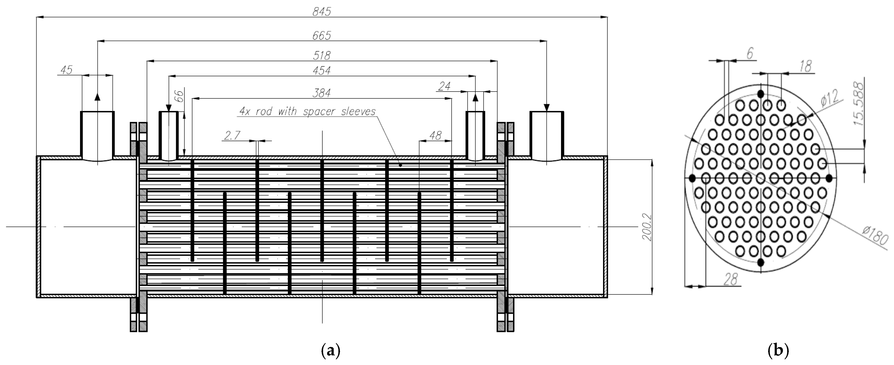
Figure 1 shows the details of the STHEx, which were examined in [28] and served as the database for the present study. The shell and the baffles were fabricated from stainless steel, while the tubes forming the bundle were made of copper.

Table 1. Geometry and operating conditions of the tested STHEx.

Item	Value/Type
Shell inner diameter	200.2 mm
Length of shell	518 mm
Total tube number	85
OD/ID tube diameter	12/10 mm
Tube layout	Triangular (30°)
Tube pitch	1.5
Total number of baffles	9
Baffle cut	25%
Central baffle spacing	48 mm
Inlet and outlet sections	67 mm
Hot fluid mass flow rate	1–3 kg/s
Cold fluid mass flow rate	3 kg/s
Inlet hot fluid temperature	35–79 °C
Cold fluid inlet temperature	7.5–11 °C

presents the geometric parameters of the tested STHEx and the operating conditions.

Table 2. The diameters of the holes in the baffles and the diameters of the baffles.

Run	${\mathit{\delta }}_{\mathit{d}} = \frac{{\mathit{d}}_{\mathit{B}}-{\mathit{d}}_{\mathit{o}}}{2}$	${\mathit{d}}_{\mathit{B}}$	${\mathit{\delta }}_{\mathit{D}} = \frac{{\mathit{D}}_{\mathit{s}}-{\mathit{D}}_1}{2}$	${\mathit{D}}_1$	Flow Configuration
A	0.0	0.0120	0.0	0.2002	No baffle-to-tube and shell-to-baffle leakages.
B	0.00012	0.01224	0.0	0.2002	No shell-to-baffle leakage; only baffle-to-tube leakage occurred.
C1	0.00012	0.01224	0.0001	0.2000	Both shell-to-baffle and baffle-to-tube leakages were present.
C2	0.00012	0.01224	0.0007	0.1988	Both shell-to-baffle and baffle-to-tube leakages were present.
C3	0.00025	0.01250	0.0007	0.1988	Both shell-to-baffle and baffle-to-tube leakages were present.
C4	0.00025	0.01250	0.0012	0.1978	Both shell-to-baffle and baffle-to-tube leakages were present.
C5	0.00050	0.0130	0.0012	0.1978	Both shell-to-baffle and baffle-to-tube leakages were present.
C6	0.00050	0.0130	0.0025	0.1952	Both shell-to-baffle and baffle-to-tube leakages were present.

presents the clearance configurations that were investigated experimentally in [21] and for which the present calculations were performed.

The maximum overall experimental uncertainties were ±5.5% for the total pressure drop and ±10.7% for the average heat transfer coefficient.

3. Materials and Methods

3.1. The Bell–Delaware Extended Model

In the extended Bell–Delaware method, the shell-side HTC is determined using the following equation [29,30]:

$${\alpha }_s=J_C{J}_L{J}_B{J}_S{J_R\alpha }_{s,id}$$

(1)

where

α_s,id is the HTC for an ideal tube bundle.

J_C is the correction factor for baffle window flow.

J_L is the correction factor for baffle leakage effects.

J_B is the correction factor for bundle bypass effects.

J_S is the correction factor for unequal baffle spacing.

J_R is the laminar flow correction factor.

Detailed step-by-step information on how to calculate the individual components is provided in [29,30].

In the extended Bell–Delaware method, the shell-side total pressure drop in an STHEx is determined using the following equation:

$$∆P_s=∆P_F+∆P_W+∆P_E+∆P_N$$

(2)

where

$∆P_F$ is the pressure drop in all central baffle spaces.

$∆P_W$ is the pressure drop in all baffle windows.

$∆P_E$ is the pressure drop in the entrance and exit baffle spaces.

$∆P_N$ is the pressure drop in nozzles.

Detailed step-by-step information on how to calculate the individual components is provided in [29].

3.2. The VDI Model

In the VDI method, shell-side HTC is determined using the following equation [31]:

$${Nu}_s=f_w{f}_N{f}_P{f}_A{Nu}_{l,o}$$

(3)

where

${Nu}_{l,o}$ is the Nusselt number for a single tube.

$f_w$ is the correction factor for the shell-side flow configuration.

$$f_w=f_G{f}_L{f}_B$$

(4)

$f_G$ is the geometry correction factor.

$f_L$ is the leakage correction factor.

$f_B$ is the bypass correction factor.

$f_N$ is the correction factor for the number of tube rows.

$f_P$ is the correction factor for the change in physical properties in the boundary layer.

$f_A$ is the tube arrangement factor.

Detailed step-by-step information on how to calculate the individual components is provided in [31].

In the VDI method, the pressure drop in the shell side of an STHEx is determined using formula [32]:

$$∆P_s=\left(n_b-1\right)∆P_Q+2∆P_{QE}+n_b∆P_W+∆P_N$$

(5)

where

$n_b$ is the number of baffles.

$∆P_Q$ is the pressure drop in a central crossflow section between two adjacent baffles.

$∆P_{QE}$ is the pressure drop in an end crossflow section.

$∆P_W$ is the pressure drop in a window section.

$∆P_N$ is the pressure drop in both inlet and outlet nozzles.

Detailed step-by-step information on how to calculate the individual components is provided in [32].

3.3. Open Foam Formulation

Water flow in each region (the shell and the tubes) is solved using equations for variable density. In this case, the mass conservation equation takes the form:

$${\displaystyle \frac{\partial \rho }{\partial \tau }}+\mathsf{\nabla }·\left(\rho \mathit{u}\right)=0$$

(6)

where ρ is the density, and u is the velocity vector. Furthermore, a variable density version of the Navier–Stokes equation can be written as

$${\displaystyle \frac{\partial }{\partial \tau }}\left(\rho \mathit{u}\right)+\mathsf{\nabla }·\left(\rho \mathit{u}\mathit{u}\right)=\rho \mathit{g}-\mathsf{\nabla }P+\mathsf{\nabla }·\left(\mu \mathsf{\nabla }\mathit{u}\right)+\mathsf{\nabla }·\left(\mu {\mathrm{d}\mathrm{e}\mathrm{v}}_2{\left(\mathsf{\nabla }\mathit{u}\right)}^T\right)$$

(7)

where P is the pressure, µ is the dynamic viscosity, g is the acceleration vector due to gravity, dev₂ T = T − 2/3 δ trT, and δ is the unity tensor. The energy equation is written as

$${\displaystyle \frac{\partial }{\partial \tau }}\left(\rho \left(K+h\right)\right)+\mathsf{\nabla }·\left(\rho \mathit{u}\left(K+h\right)\right)={\displaystyle \frac{\partial P}{\partial \tau }}+\rho \mathit{g}·\mathit{u}+\mathsf{\nabla }·\left(\lambda \mathsf{\nabla }h\right)$$

(8)

The kinetic energy is in the form K = 1/2 ‖u‖², h is the specific enthalpy, and λ is the thermal conductivity.

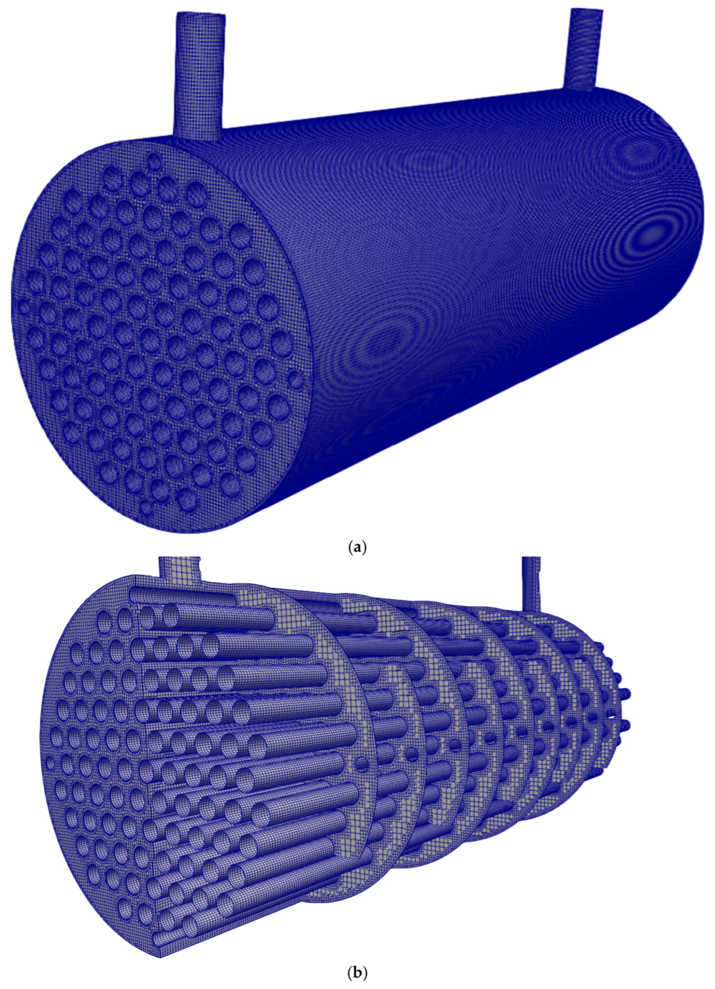
The system of Equations (6)–(8), after averaging by the RAS method, is solved for P, T, and u using the k-ω SST turbulence model [33]. The system of equations was discretized using the finite volume method, and the resulting system of algebraic equations was solved using the open-source software OpenFOAM v2312 [34]. The problem was steady-state. Convection terms are interpolated by means of limited linear schemes, and the discretized Laplacian terms take advantage of the corrected schemes. Gradients take advantage of Gaussian integration together with linear interpolation. All fluxes utilize linear interpolation. The system of equations is solved using the SIMPLE algorithm with an active momentum predictor. What is more, the pressure equation is solved by means of the GAMG solver with the DIC smoother. Furthermore, the smooth solvers with the Gauss–Seidel smoother are utilized for the velocity u components, enthalpy h, and turbulence quantities such as k and ω. Finally, the geometry of the heat exchanger was discretized using a Cartesian mesh (Figure 2a,b), resulting in a total of 9.92 million nodes.

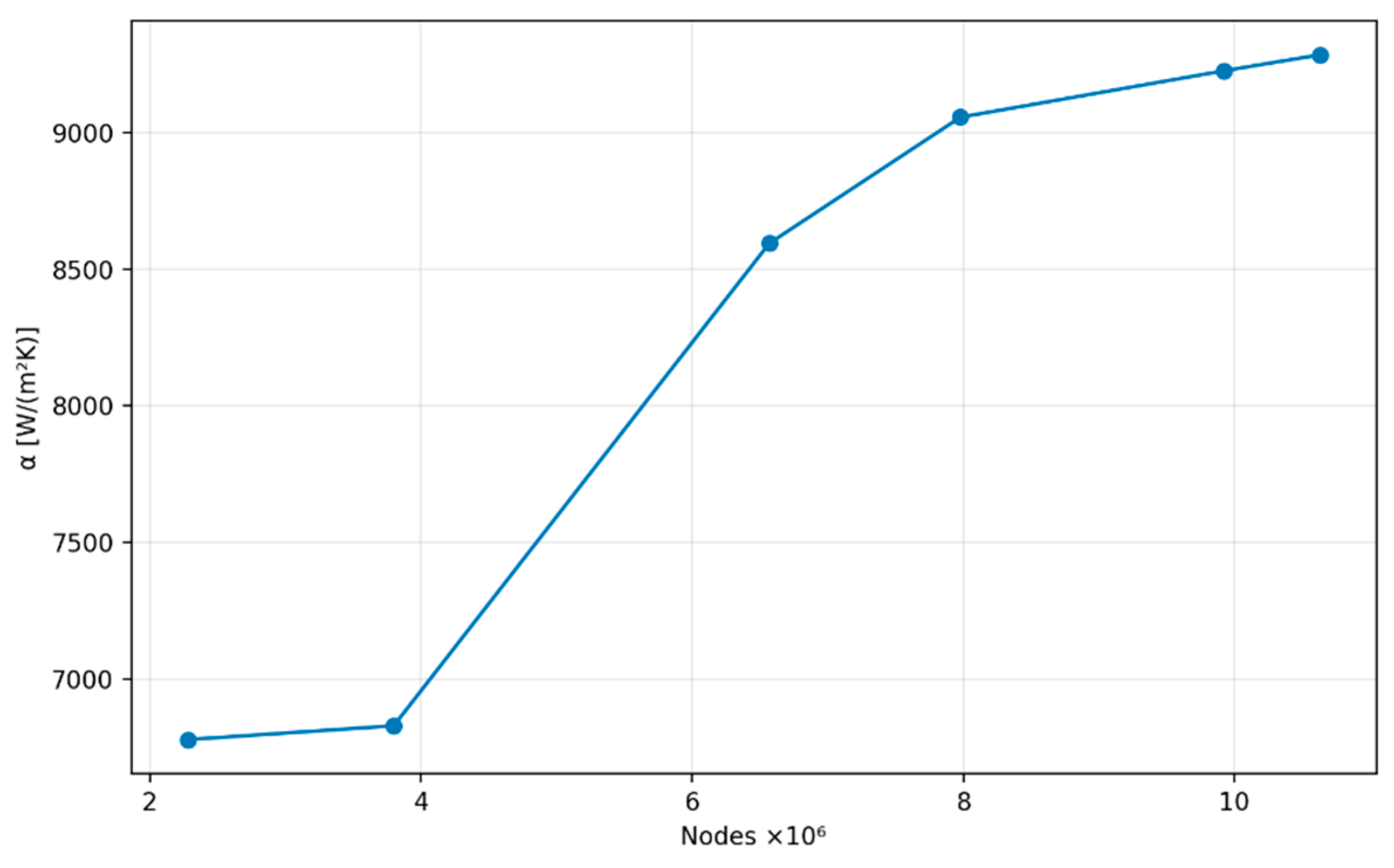
Figure 3 shows the effect of the computational mesh on the HTC. Six cases were considered, ranging from the smallest mesh with 2.2 million nodes to the largest, which has 10.6 million nodes.

As shown in Figure 3, the HTC changes significantly as the mesh size increases up to approximately 8 million nodes. Further refinement to about 9 million nodes does not lead to significant changes, and beyond 10 million nodes, the changes become negligible. Therefore, a mesh with 9.9 million nodes was selected for further calculations. The effect was studied for a mass flow rate in the shell of ${\dot{m}}_H$ = 2.707 kg/s and an inlet temperature of t_H,in = 77.82 °C.

The HTC, α, was calculated using the following equation:

$$\alpha ={\displaystyle \frac{\dot{Q}}{A_o\left(T_w-T_r\right)}}$$

(9)

where $\dot{Q}$ is the heat flow rate obtained from the CFD calculations, $A_o$ is the external surface of the tube bundle, T_w is the average surface temperature of the tubes from the CFD calculations, and T_r is the reference temperature. This temperature is the arithmetic mean of the inlet and outlet temperatures. The inlet temperature is a boundary condition, while the outlet temperature is derived from CFD calculations and is understood as the mass average of the temperature field at the outlet surface

3.4. Ansys Fluent Formulation

The numerical simulations were performed using ANSYS Fluent 19.3 [35]. The flow field was described by the Reynolds-Averaged Navier–Stokes (RANS) equations, obtained through time-averaging of the instantaneous conservation equations. The continuity equation for incompressible, steady-state flow is:

$$\mathsf{\nabla }·\mathit{u}=0$$

(10)

where $\mathit{u}$ is the velocity vector

The momentum equation is given by:

$$\rho \left(\mathit{u}·\mathsf{\nabla }\mathit{u}\right)=-\mathsf{\nabla }P+\mathsf{\nabla }·\mathit{\tau }$$

(11)

where $\rho$ is the density, P is the static pressure, and $\mathit{\tau }$ is the stress tensor (incorporating both molecular and turbulent viscosities).

The energy equation is formulated as:

$$\rho c_p\left(\mathit{u}·\mathsf{\nabla }T\right)=\mathsf{\nabla }·\left({\lambda }_{eff}\mathsf{\nabla }T\right)$$

(12)

where T is the temperature and λ_eff denotes the effective thermal conductivity (material conductivity and turbulent thermal conductivity). For steady-state conditions of simulations, the transient terms are neglected.

The inlet boundary conditions were defined by specifying the mass flow rate and temperature for both the shell and tube sides:

$$\dot{m}=const, T=T_{in}$$

(13)

A mass flow rate boundary condition was imposed at the outlet to enhance numerical stability. A no-slip boundary condition was applied at all solid walls, with the velocity set to zero (u = 0). The standard k–ε turbulence model, combined with enhanced wall treatment, was employed to improve near-wall accuracy.

The governing equations were discretized using the finite volume method. Second-order spatial discretization schemes were adopted to improve numerical accuracy. Pressure–velocity coupling was resolved using the SIMPLE algorithm. Convergence was considered achieved when the residuals dropped below 10⁻⁶ for the energy equation and 10⁻⁵ for all other equations, and when monitored integral parameters, namely the pressure drop and heat transfer rate, reached stable values.

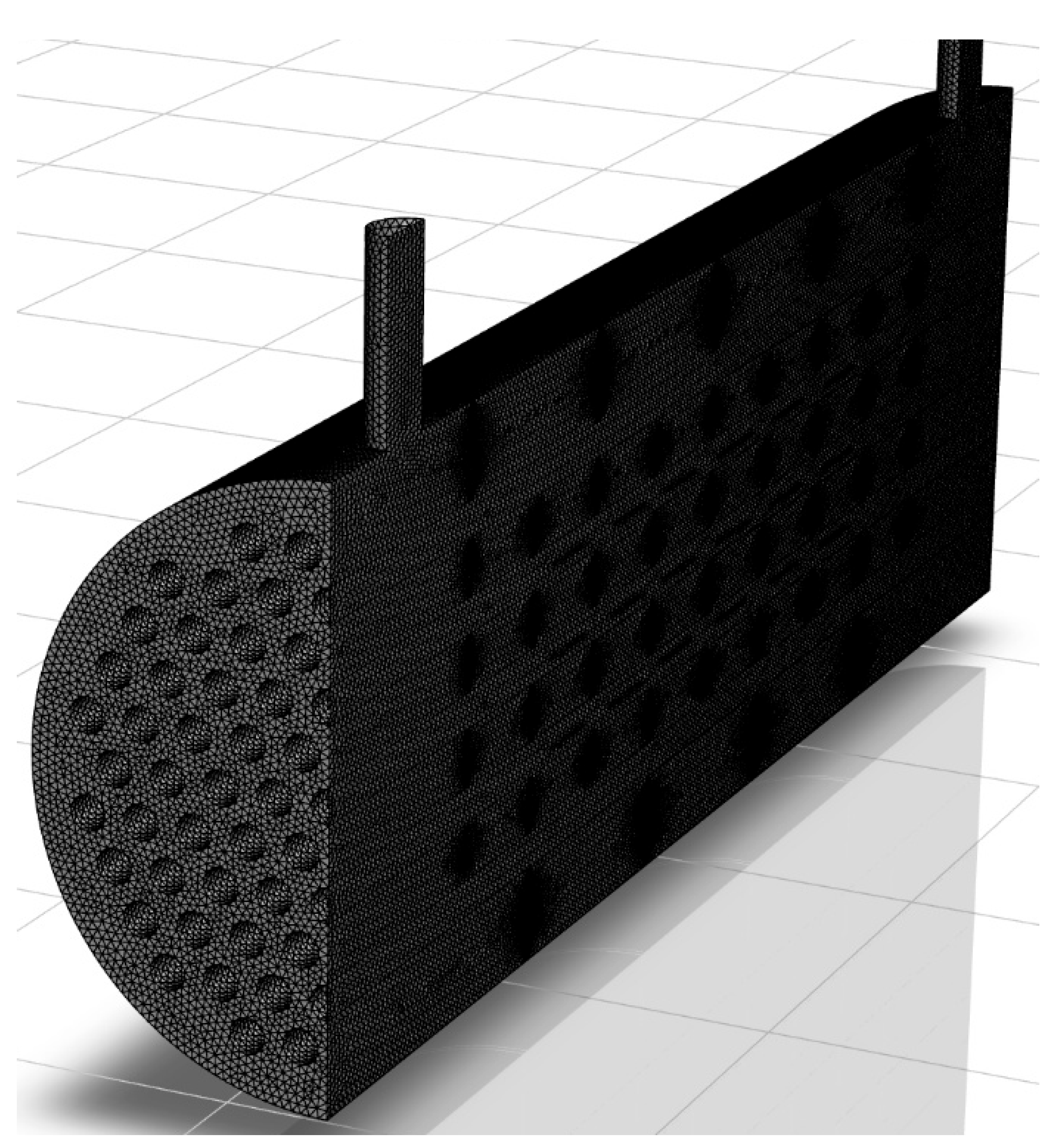
The computational model of the STHEx was developed in the Ansys Gambit 2.4.6 preprocessor, as shown in Figure 4. An unstructured mesh consisting of tetrahedral volumes was generated to accurately capture the complex geometry of the heat exchanger and the baffle configuration. Owing to the symmetry of the computational domain, only half of the exchanger volume was considered in the simulations. The resulting mesh for this half-domain contained 4.388 million finite volumes.

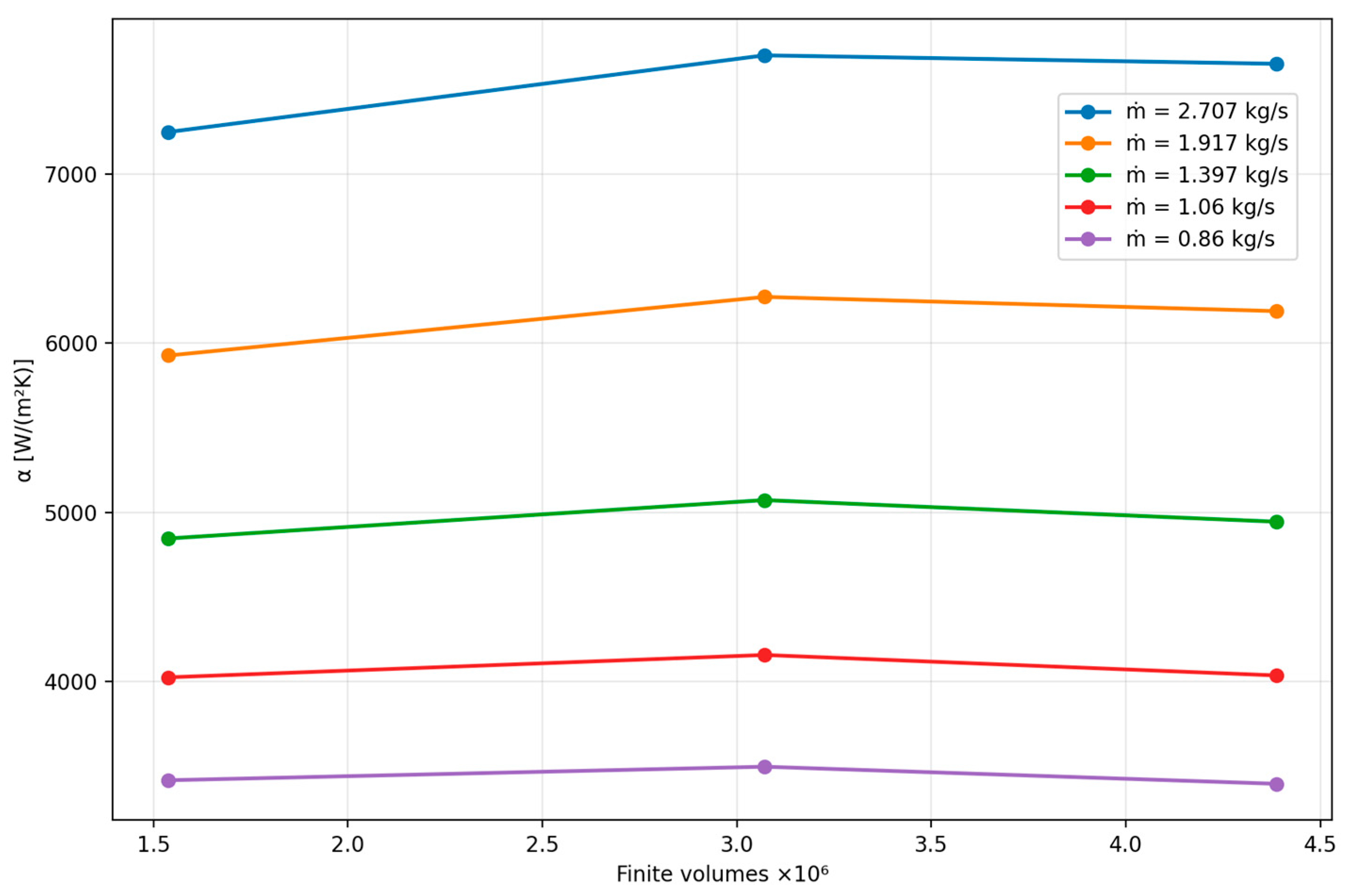
Figure 5 illustrates the effect of the number of finite volumes on the average HTC. Three meshes were considered for mass flow rates, ranging from the minimum to the maximum value. For each mass flow rate, the number of finite volumes ranged from 1.538 million to 4.388 million.

As shown in Figure 5, the HTC increased slightly as the number of finite volumes was raised from 1.538 million to 3.071 million, with the increase being more pronounced at higher mass flow rates. The difference in HTC values between the meshes with 4.388 million and 3.071 million finite volumes did not exceed 3% for any of the investigated mass flow rates. Therefore, the mesh with 4.388 million finite volumes was selected for the calculations, as it did not result in a significant increase in computational time.

3.5. Aspen Exchanger Design and Rating

Aspen Exchanger Design and Rating (Aspen EDR) V15.0 is proprietary software, in which the specific correlations are not available in the open literature [36]. The shell-side thermohydraulic analysis is based on the Stream Analysis Method, originally proposed by Tinker [11,12] and further developed by Palen and Taborek [37]. The heat transfer coefficients are computed at each baffle space from proprietary Nusselt number and friction factor correlations [36]. The total pressure drop on each side comprises frictional, gravitational, and acceleration (momentum) contributions. On the shell side, the frictional component is further decomposed into nozzle, bundle entrance and exit, crossflow, and baffle window terms [36].

3.6. Properties of the Tested Fluids

The thermophysical properties of water used as the working fluid were determined using correlations developed based on [38]. The following equations were used to calculate the individual properties:

-

Dynamic viscosity

$$\mu =2.2551418931-3.3948447154\times {10}^{-2}T+2.0532435429\times {10}^{-4}{T}^2-6.2294811154\times {10}^{-7}{T}^3+9.4740755112\times {10}^{-10}{T}^4-5.7750953816\times {10}^{-13}{T}^5$$

(14)

-

Thermal conductivity

$$\lambda =2.7689426052\times 10-4.1570211623\times {10}^{-1}T+2.4968651122\times {10}^{-3}{T}^2-7.3889761073\times {10}^{-6}{T}^3+1.0839020278\times {10}^{-8}{T}^4-6.3292341999\times {10}^{-12}{T}^5$$

(15)

-

Density

$$\rho =-5.8593636805\times {10}^3+9.8968557714\times 10T-5.7474749375\times {10}^{-1}{T}^2+1.6856053180\times {10}^{-3}{T}^3-2.4989340377\times {10}^{-6}{T}^4+1.4908022754\times {10}^{-9}{T}^5$$

(16)

-

Specific heat

$$c_p=1.8561445426\times {10}^5-2.7374285462\times {10}^{3}T+1.6544683581\times 10T^2-5.0060497615\times {10}^{-2}{T}^3+7.5807970466\times {10}^{-5}{T}^4-4.5941525532\times {10}^{-8}{\mathrm{T}}^5$$

(17)

-

Prandtl number

$$\mathit{pr}=1130.643576-10.068594T+0.030127T^2-3\times {10}^{-5}{T}^3$$

(18)

The applicability range of Equations (14)–(18) is 10 ≤ t ≤ 80 °C. Within this temperature interval, the coefficient of determination, R², is equal to 1.00000 for dynamic viscosity, thermal conductivity, and density, while for specific heat it is 0.99987. To ensure accurate evaluation of the thermophysical properties, all terms in the equations, as well as the specified number of significant figures, must be retained.

4. Results

4.1. A Quasi-Ideal Heat Exchanger

In a quasi-ideal STHEx, it is assumed that there is no fluid leakage either between the baffles and the tubes or between the baffles and the shell. However, a gap remains between the tube bundle and the shell, allowing part of the fluid to bypass the tube bundle and, consequently, not participate in heat transfer.

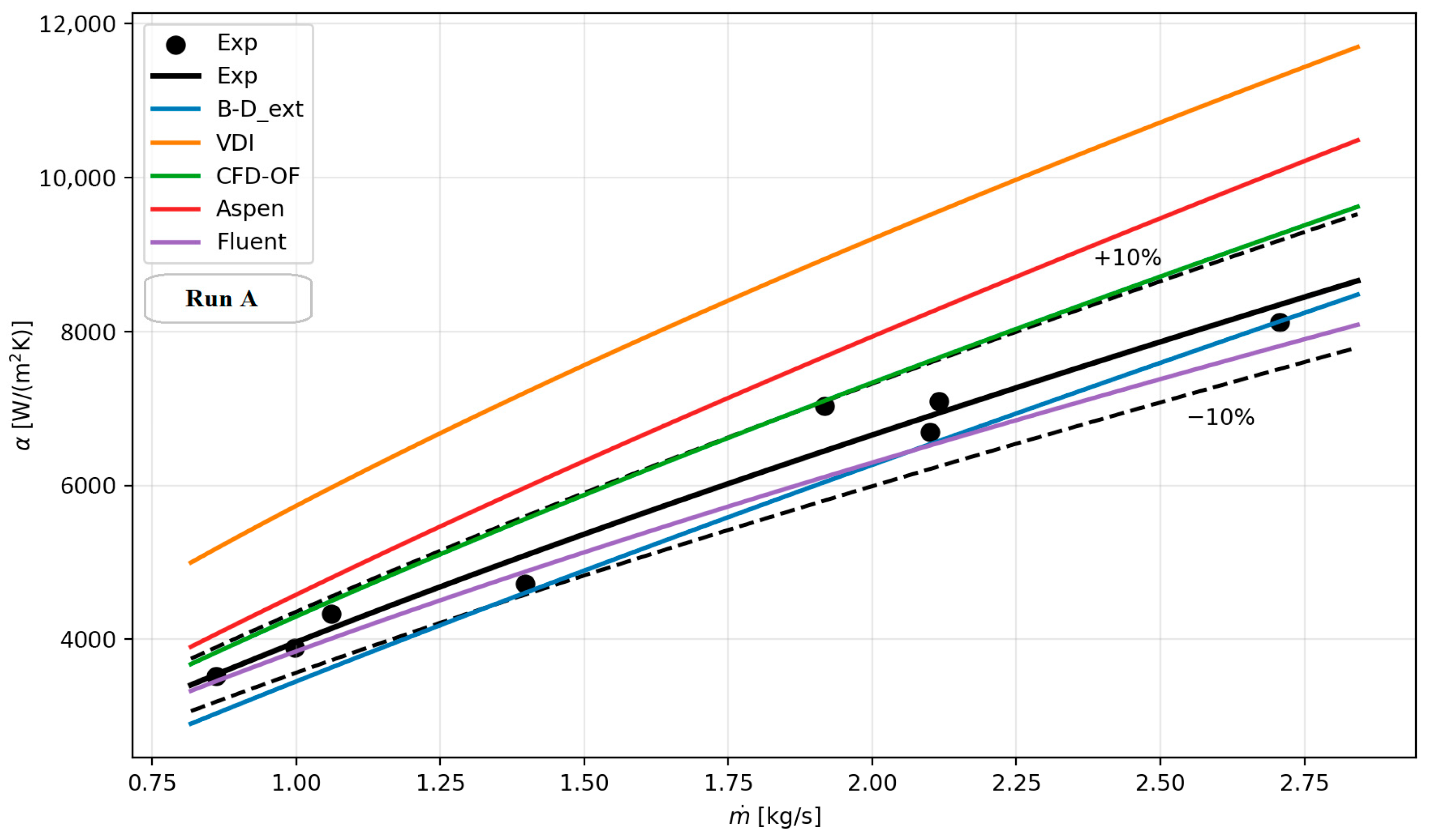
Figure 6 shows a comparison of the shell-side HTC calculated using the presented methods with the available experimental data [28] for run A (Table 2).

As shown in Figure 6, all experimental points (black dots) lie within ±10% of the mean value represented by the solid black line. The experimental results are reproduced accurately by the Bell–Delaware extended method and by calculations performed using Ansys Fluent software. The OpenFOAM CFD simulations, Aspen EDR package, and the VDI method overpredict the mean experimental HTC by about 10%, 18%, and 33%, respectively.

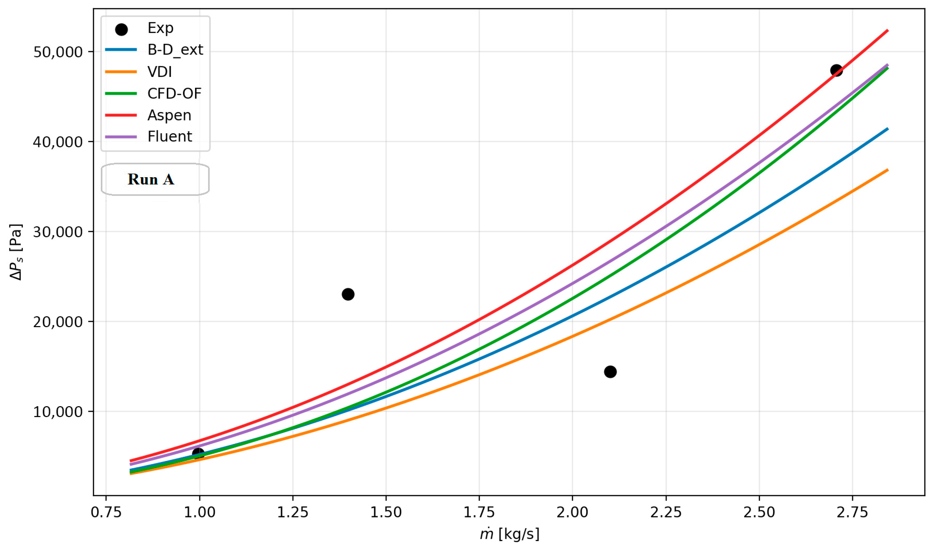
Figure 7 shows a comparison of the total pressure drop (ΔP_s) calculated using the presented methods with the available experimental data [28] for run A (Table 2).

As shown in Figure 7, Aspen EDR predicts the highest shell-side pressure drop (ΔP_s), whereas the VDI method gives the lowest. Aspen EDR—except for one point at ${\dot{m}}_H=2.1 \mathrm{k}\mathrm{g}/\mathrm{s}$—most accurately reproduces the experimental data. The simulation results obtained with both CFD methods (the green line—OpenFOAM; the purple line—Ansys Fluent, in Figure 7) are similar to each other and lie between the predictions made using the Aspen EDR package and the Bell–Delaware method.

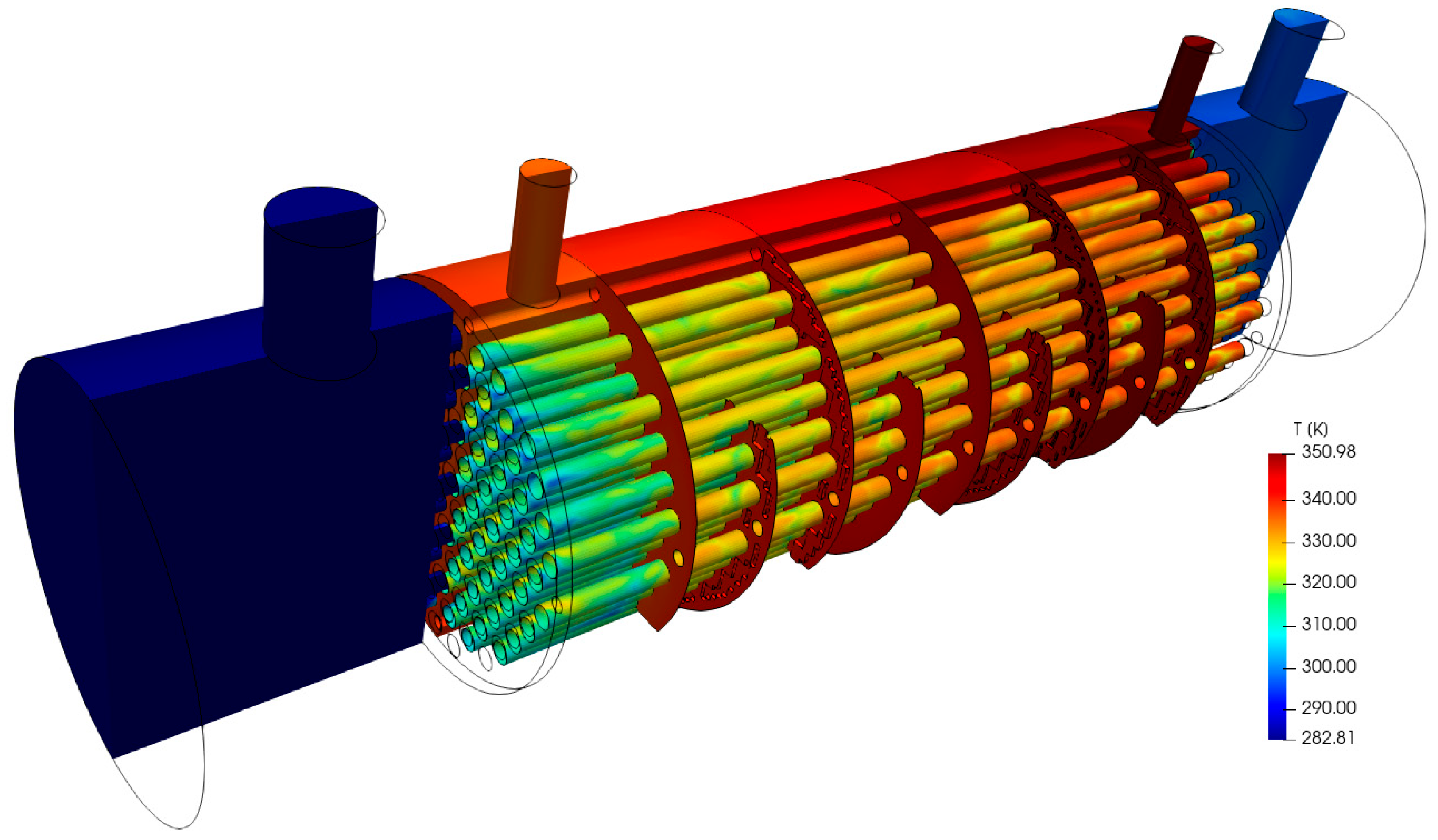
Figure 8 shows the temperature distribution within the shell and along the outer surfaces of the tubes for hot and cold water mass flow rates of ${\dot{m}}_H$ = 2.707 kg/s and ${\dot{m}}_C=$ 3.173 kg/s, respectively. The corresponding inlet temperatures were t_H,in = 77.82 °C for the hot water and t_C,in = 9.81 °C for the cold water. The shell’s outer surface was removed to allow visualization of the temperature distribution on the tubes.

As shown in Figure 8, the temperature distribution on the surface of the tubes is highly non-uniform along the entire length of the shell. Additional non-uniformity in the distribution is also visible near the hot water inlet.

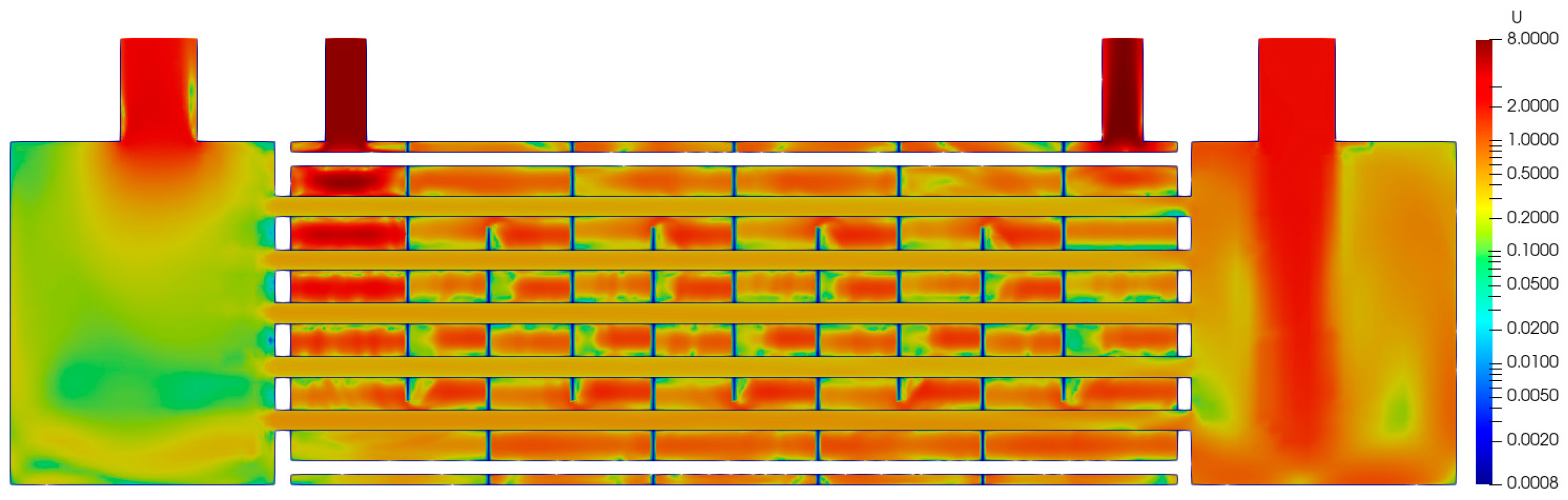
Figure 9 presents the velocity distribution in the longitudinal section for both the shell and the tubes, using the same parameter set as for the temperature field, i.e., for hot and cold water mass flow rates of ${\dot{m}}_H=$ 2.707 kg/s and ${\dot{m}}_C=$3.173 kg/s, respectively, and the corresponding inlet temperatures of t_H,in = 77.82 °C for the hot water and t_C,in = 9.81 °C for the cold water.

The velocity distribution in Figure 9 is presented on a logarithmic scale to highlight variations across the full velocity range. On the shell side, the velocity field is highly non-uniform due to the presence of the baffles and the tube bundle. The inlet jet decelerates rapidly as it impinges on the bundle. As expected, the highest velocities occur in the inlet and outlet nozzles. In the velocity map (Figure 9), the blue region, corresponding to near-zero velocities, is absent, indicating that no dead zones are present in the tested heat exchanger.

4.2. Heat Exchanger with Clearances

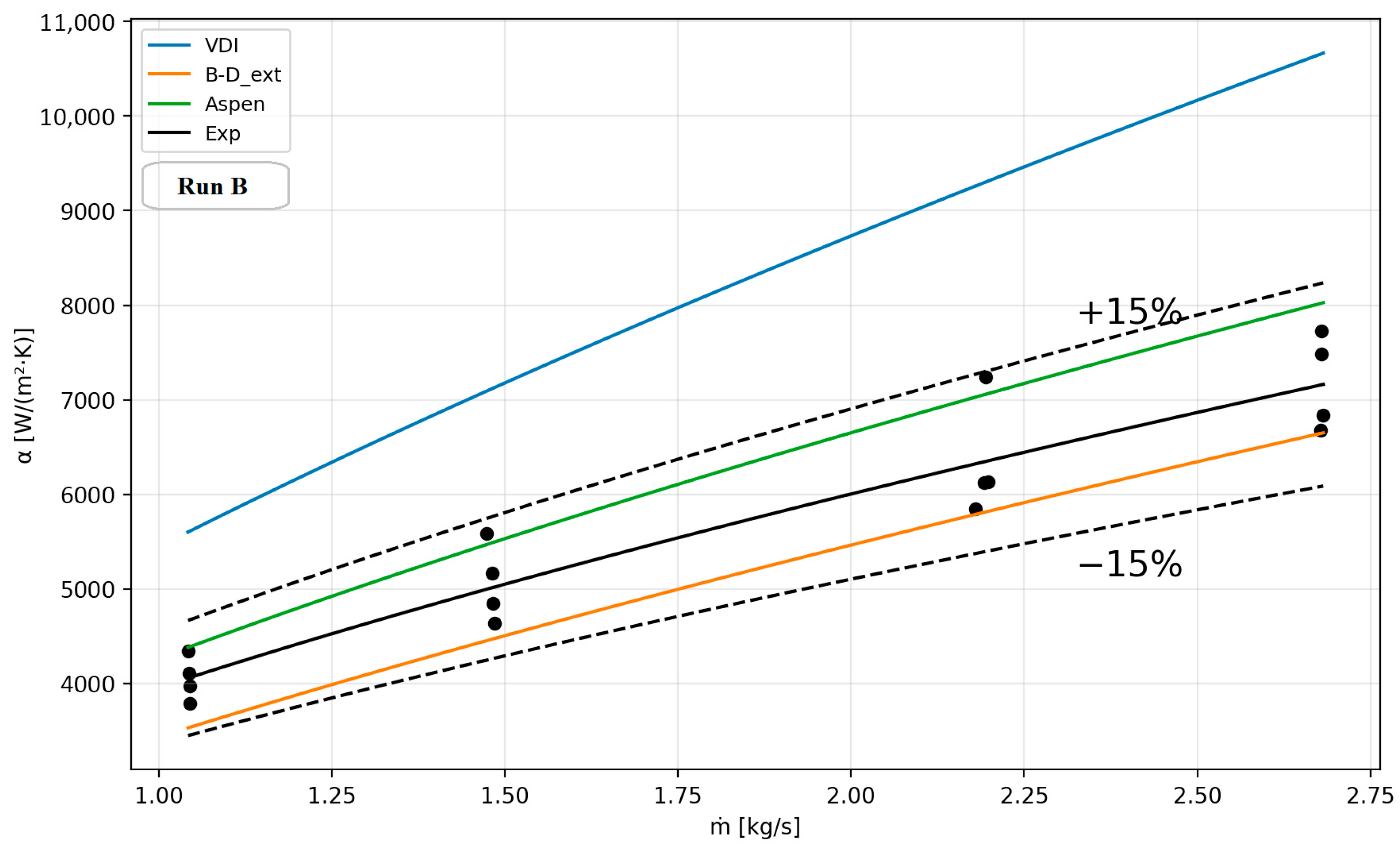
Figure 10 shows a comparison of the shell-side HTC calculated using the presented methods with the available experimental data [28] for run B (Table 2).

As shown in Figure 10, the experimental points deviate by no more than ±15% from the approximation line obtained using the least-squares method. The Bell–Delaware extended method underpredicts the experimental data by no more than about 7%, whereas Aspen EDR overpredicts it by no more than about 8%. The VDI method significantly overpredicts the experimental data, with a maximum of 37% at higher mass flow rates.

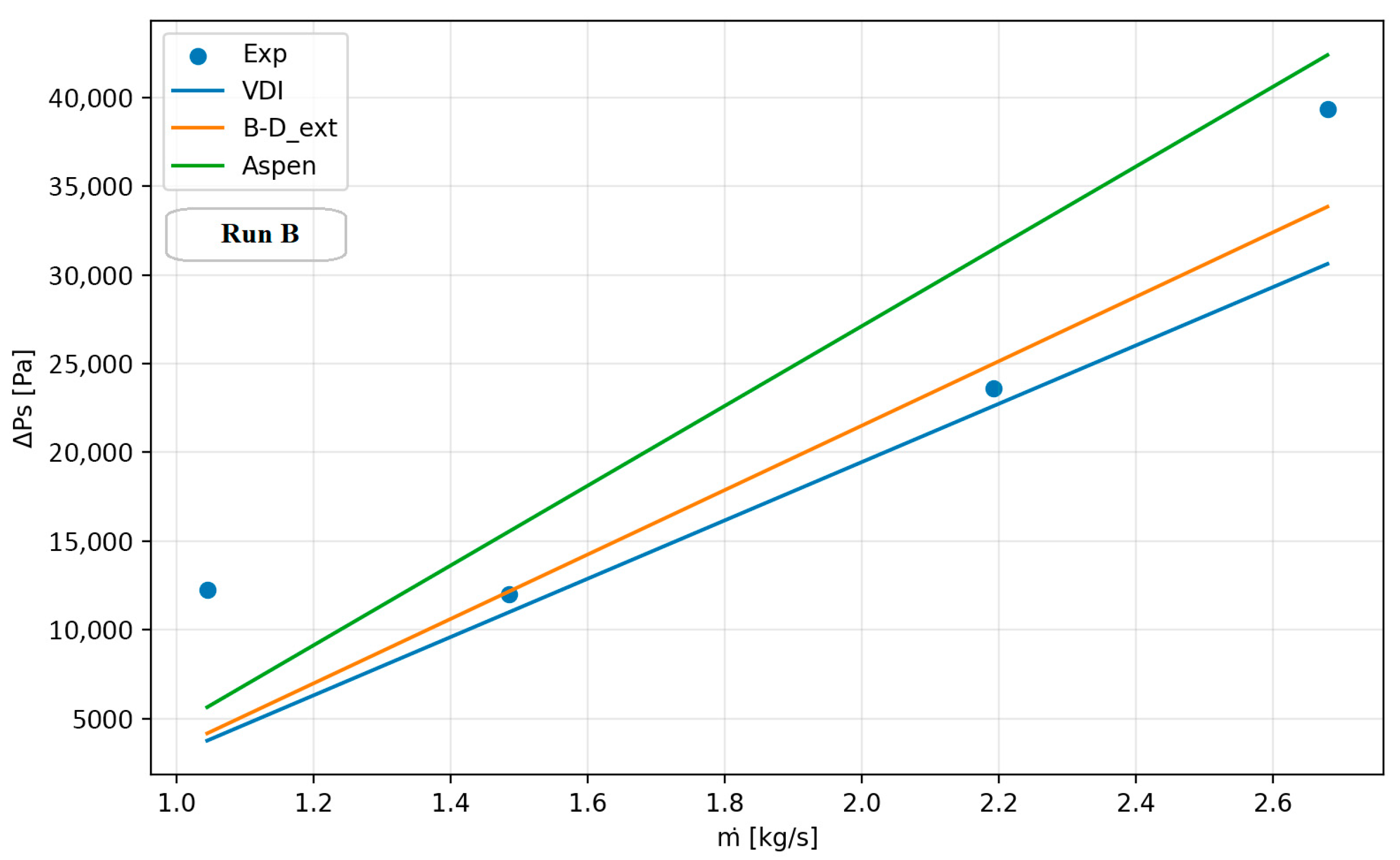
Figure 11 shows a comparison of the total pressure drop (ΔP_s) calculated using the presented methods with the available experimental data [28] for run B (Table 2).

As shown in Figure 11, similarly to the ideal STHEx case (Figure 7), the difference in the predicted ΔP_s values between the Bell–Delaware extended method and the VDI method is below 10%, with the Bell–Delaware extended method showing better agreement with the experimental data.

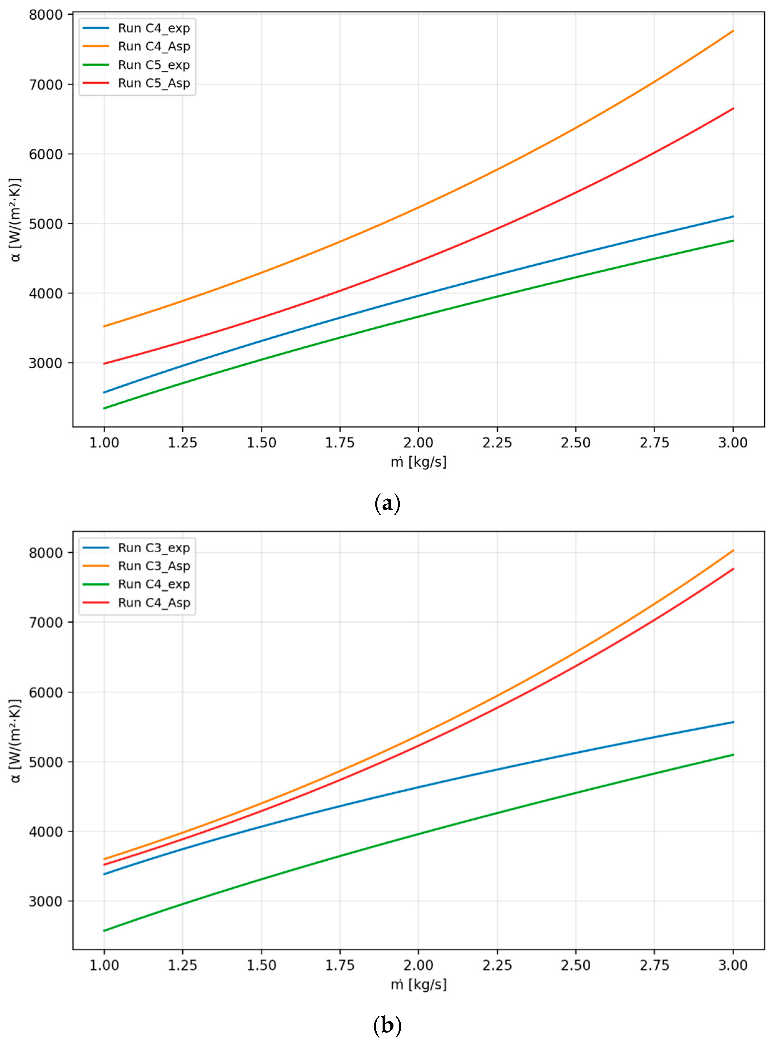
Figure 12 shows the impact of the baffle-to-tube (Figure 12a) and shell-to-baffle clearance (Figure 12b) on the shell-side HTC.

As shown in Figure 12a, for the same shell-to-baffle clearance (δ_D = 1.2 mm), the experimental data indicate that increasing the baffle-to-tube clearance from δ_d = 0.25 mm to δ_d = 0.5 mm, that is, by 100%, reduces the shell-side HTC by only about 6.8%. Conversely, for the same baffle-to-tube clearance (δ_d = 0.25 mm), increasing the shell-to-baffle clearance from δ_D = 0.7 mm to δ_D = 1.2 mm (i.e., by 71%) resulted in a decrease in the shell-side HTC by about 24%; Figure 12b. The calculations performed using Aspen EDR, although they predict a much higher shell-side HTC than the experimental data—especially at a higher mass flow rate—also indicate a lower sensitivity to an increase in the shell-to-baffle clearance (Figure 12b) than to an increase in the baffle-to-tube clearance (Figure 12a). The corresponding reductions in the shell-side HTC were about 17% and 4%, respectively.

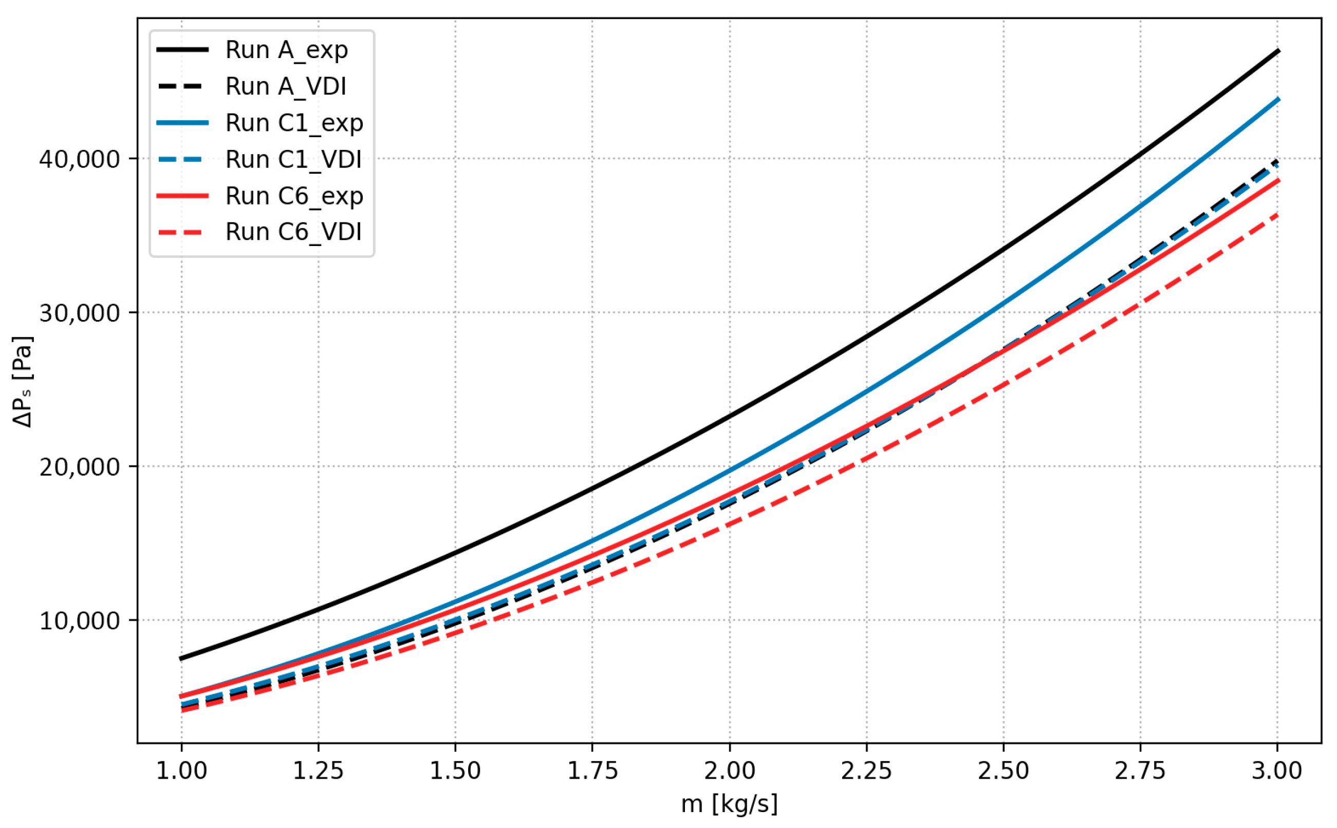
Figure 13 shows the combined effect of the baffle-to-tube and shell-to-baffle clearances (from minimum to maximum; Runs A, C1, and C6 in Table 2) on the total pressure drop determined experimentally (solid lines) and calculated using the VDI method (dashed lines).

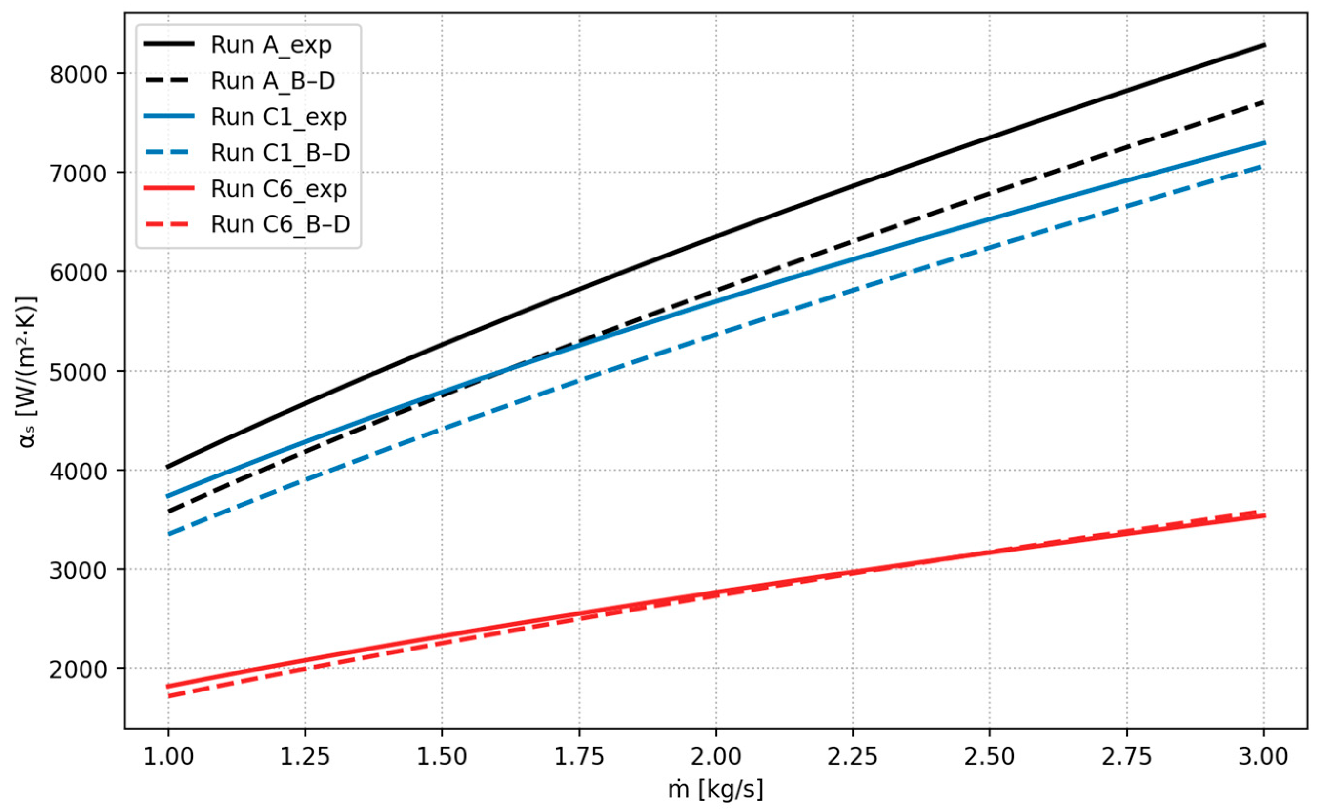
As shown in Figure 13, the total pressure drop for the case with the maximum baffle-to-tube and shell-to-baffle clearances is about 12% lower than that for the minimum-clearance case C1. This is beneficial in terms of lower pumping power; however, leakage through these clearances deteriorates heat transfer, because a smaller portion of the fluid is directed perpendicular to the tube bundle. This is shown in Figure 14, which illustrates the combined effect of the baffle-to-tube and shell-to-baffle clearances (from minimum to maximum; Runs A, C1, and C6 in Table 2) on the shell-side HTC, determined experimentally (solid lines) and calculated using the extended Bell–Delaware method (dashed lines).

As shown in Figure 14, the shell-side HTC for the case with the maximum baffle-to-tube and shell-to-baffle clearances is about 52% lower than that for the ideal case. It is important to note that as the clearances increase, the discrepancy between the measured and calculated values decreases significantly. While for the ideal STHEx, the difference between the measured and calculated shell-side HTC (black solid and dashed lines in Figure 14) was about 10%, for the maximum clearances (orange solid and dashed lines in Figure 14), it was negligibly small.

5. Conclusions

The research conducted allows us to draw the following conclusions:

• The VDI method gives the highest shell-side HTC compared to the other tested methods. Characteristically, it overestimates the shell-side HTC the smaller the clearances are. The VDI method overestimates the heat transfer coefficient by approximately 33% and underestimates the pressure drop by about 20%, relative to the experimental data.
• The extended Bell–Delaware method reproduces the experimental data accurately for both shell-side HTC and pressure drop, although it most often slightly underestimates them. The extended Bell–Delaware method shows the highest agreement with the experimental results, reproducing the data within a ±10% band.
• Aspen EDR accurately reproduces both the experimental shell-side HTC and the pressure drop over the entire range of tested clearances, with a discrepancy not exceeding ±17%.
• CFD simulations (using both OpenFOAM and Ansys Fluent), conducted only for a quasi-ideal STHEx (without leakages), showed good agreement with the experimental data. The OpenFOAM and Ansys Fluent simulations reproduced a mean HTC within a ±10% range. Regarding the shell-side pressure drop, the OpenFOAM and Ansys Fluent calculations yielded values approximately 4% lower than those predicted by Aspen EDR, which provided the most accurate agreement with the experimental data. However, the computation time for a single set of input data exceeded 12 h (Xeon 8173m processor, 13/28 cores involved); therefore, this approach is better suited to optimizing STHEx designs rather than being used during the design stage, especially in the preliminary design stage.
• The experiments and calculations confirmed both a reduction in flow resistance (pressure drop) and the shell-side HTC as the clearances’ cross-sectional area increased. However, while the maximum pressure drop decreased by about 12%, the shell-side HTC decreased by as much as 52% compared to the quasi-ideal STHEx. Such a small reduction in pressure drop results from the fact that the main contribution to the total pressure drop comes from the nozzle pressure drop due to expansion at the inlet nozzle and contraction at the outlet nozzle, which is practically independent of the clearance size. Increasing the cross-sectional area of the baffle-to-tube and shell-to-baffle clearances reduces the fraction of fluid flowing perpendicular (which is desirable) to the tubes and increases the fraction of fluid flowing parallel to the tubes, which leads to a significant decrease in shell-side HTC.
• From a practical point of view, the reduction in pressure drop, resulting from the increase in the clearances’ cross-sectional area, leads to a decrease in pumping power and, consequently, to lower heat-exchanger operating costs. On the other hand, a decrease in the HTC (in the analyzed case, even exceeding 50%) may mean that the heat exchanger must have a larger heat transfer area, which results in greater material consumption and higher energy use during its manufacturing. Therefore, both the long-term operating costs and capital costs of the heat exchanger should be evaluated very carefully, while also taking into account the significantly higher manufacturing costs of a heat exchanger with small clearances, especially in the case of a large number of baffles and tubes in the bundle.

Future work will focus on thermal and hydrodynamic studies of a water/EG mixture in shell-and-tube heat exchangers with segmental baffles, while considering a wider range of mass flow rates and examining in more detail the effects of the tube bundle diameter and nozzle diameter on pressure drop and shell-side HTC.

References

1. Master, B.I.; Chunangad, K.S.; Boxma, A.J.; Kral, D.; Stehlík, P. Most Frequently Used Heat Exchangers from Pioneering Research to Worldwide Applications. Heat Transf. Eng. 2006, 27, 4–11. [Google Scholar] [CrossRef]
2. Sagar, J.P.; Ankith, B.; Rao, P.S.; Reddy, P.R.; Elipey, M.K. A review on heat transfer enhancement methods for a heat exchanger. AIP Conf. Proc. 2022, 2648, 040005. [Google Scholar] [CrossRef]
3. Marzouk, S.A.; Abou Al-Sood, M.M.; El-Said, E.M.S.; Younes, M.M.; El-Fakharany, M.K. A comprehensive review of methods of heat transfer enhancement in shell and tube heat exchangers. J. Therm. Anal. Calorim. 2023, 148, 7539–7578. [Google Scholar] [CrossRef]
4. Gobinathan, S.N.; Aziz, A.A.; Oumer, A.N.; Taib, M.Y.; Alias, A.B.S. A Review on Heat Transfer Enhancement in a Heat Exchanger. J. Adv. Res. Fluid Mech. Therm. Sci. 2024, 122, 130–145. [Google Scholar] [CrossRef]
5. Bichkar, P.; Dandgaval, O.; Dalvi, P.; Godase, R.; Dey, T. Study of Shell and Tube Heat Exchanger with the Effect of Types of Baffles. Procedia Manuf. 2018, 20, 195–200. [Google Scholar] [CrossRef]
6. Arani, A.A.A.; Moradi, R. Shell and tube heat exchanger optimization using new baffle and tube configuration. Appl. Therm. Eng. 2019, 157, 113736. [Google Scholar] [CrossRef]
7. Omar, H.; Alfaraw, S.; El-sawi1, A.; Alobeidy, H. Study the Effect of Baffle Spacing on Heat Transfer and Pressure Drop in Shell and Tube Heat Exchanger. J. Adv. Res. Numer. Heat Transf. 2021, 6, 22–30. [Google Scholar]
8. Marzouk, S.A.; Abou Al-Sood, M.M.; El-Fakharany, M.K.; El-Said, E.M.S. A comparative numerical study of shell and multi-tube heat exchanger performance with different baffles configurations. Int. J. Therm. Sci. 2023, 179, 107655. [Google Scholar] [CrossRef]
9. Mohammadzadeh, A.M.; Jafari, B.; Hosseinzadeh, K. Comprehensive numerical investigation of the effect of various baffle design and baffle spacing on a shell and tube heat exchanger. Appl. Therm. Eng. 2024, 249, 123305. [Google Scholar] [CrossRef]
10. Tinker, T. Shell Side Characteristics of Shell and Tube Heat Exchanger, Parts I-III, General Discussion of Heat Transfer; Institution of Mechanical Engineers: London, UK; ASME: New York, NY, USA, 1951; pp. 84–110. [Google Scholar]
11. Tinker, T. Shell-Side Characteristics of Shell and Tube Heat Exchanger. J. Heat Transf. 1958, 80, 36–52. [Google Scholar]
12. Bell, K.J. Exchanger Design—Based on the Delaware Research Program. Petro/Chem Eng. 1960, 32, C-26–C-40c. [Google Scholar]
13. Bell, K.J. Final Report of the Cooperative Research Program on Shell and Tube Heat Exchangers; Bulletin No. 5; University of Delaware Engineering Experimental Station: Newark, DE, USA, 1963. [Google Scholar]
14. Gaddis, E.S.; Gnielinski, V. Pressure drop on the shell side of shell-and-tube heat exchangers with segmental baffles. Chem. Eng. Process 1977, 36, 149–159. [Google Scholar] [CrossRef]
15. Gnielinski, V.; Gaddis, E.S. Berechnung des mittlerenWärmeübergangskoeffizienten im Außenraum von Rohrbündelwärmeaustauschern mit Segment-Umlenkblechen. Vt Verfahrenstechnik 1978, 12, 211–217. [Google Scholar]
16. Estupiñan-Campos, J.; Quitiaquez, W.; Nieto-Londono, C.; Quitiaquez, P. Numerical simulation of the heat transfer inside a shell and tube heat exchanger considering different variations in the geometric parameters of the design. Energies 2024, 17, 691. [Google Scholar] [CrossRef]
17. Khan, A.; Shah, I.; Gul, W.; Khan, T.A.; Ali, Y.; Masood, S.A. Numerical and experimental analysis of shell and tube heat exchanger with round and hexagonal tubes. Energies 2023, 16, 880. [Google Scholar] [CrossRef]
18. Hoang, H.M.K.; Cao, H.-L.; Pham, P.M.Q.; Hajjar, A.; Nguyen, V.L. A novel shell-and-tube heat exchanger design with alternative inclined baffles. Case Stud. Therm. Eng. 2025, 65, 105542. [Google Scholar] [CrossRef]
19. Waleed, M.; Naqvi, S.M.A.; Mustafa, H.; Al Mesfer, M.K.; Danish, M.; Irshad, K.; Shahzad, H. Numerical analysis of shell and tube heat exchanger with combination of different baffles. Case Stud. Therm. Eng. 2025, 65, 105658. [Google Scholar] [CrossRef]
20. Adebayo, J.K.; Dare, A.A.; Petinrin, M.O. Performance characteristics of shell and tube heat exchanger using sectoral baffle. J. Eng. Appl. Sci. 2025, 72, 13. [Google Scholar] [CrossRef]
21. Prithiviraj, M.; Andrews, M.J. Comparison of a Three-Dimensional Numerical Model with Existing Methods for Prediction of Flow in Shell-and-Tube Heat Exchangers. Heat Transf. Eng. 1999, 20, 15–19. [Google Scholar]
22. Kapale, U.C.; Satish Chand, S. Modeling for shell-side pressure drop for liquid flow in shell-and-tube heat exchanger. Int. J. Heat Mass Transf. 2006, 49, 601–610. [Google Scholar] [CrossRef]
23. Parikshit, B.; Spandana, K.R.; Krishna, V.; Seetharam, T.R.; Seetharamu, K.N. A simple method to calculate shell side fluid pressure drop in a shell and tube heat exchanger. Int. J. Heat Mass Transf. 2015, 84, 700–712. [Google Scholar] [CrossRef]
24. Kücük, H.; Ünverdi, M.; Yılmaz, M.S. Experimental investigation of shell side heat transfer and pressure drop in a mini-channel shell and tube heat exchanger. Int. J. Heat Mass Transf. 2019, 143, 118493. [Google Scholar] [CrossRef]
25. Abdelkader, B.A.; Zubair, S.M. The Effect of a Number of Baffles on the Performance of Shell-and-Tube Heat Exchangers. Heat Transf. Eng. 2019, 40, 39–52. [Google Scholar] [CrossRef]
26. Alperen, M.A.; Kayabaşi, E.; Hüseyin Kurt, H. Detailed comparison of the methods used in the heat transfer coefficient and pressure loss calculation of shell side of shell and tube heat exchangers with the experimental results. Energy Sources Part A Recovery Util. Environ. Eff. 2023, 45, 5661–5680. [Google Scholar] [CrossRef]
27. Di Bono, G.; Corcione, M.; Quintino, A. Systematic comparative analysis of Kern and Bell-Delaware methods for the design of shell-and-tube heat exchangers. Appl. Therm. Eng. 2025, 278, 127327. [Google Scholar] [CrossRef]
28. Mahdi, A.S.M. Effect of Baffle Gaps on Heat Transfer in a Shell-and-Tube Heat Exchanger. Ph.D. Thesis, Gdańsk University of Technology, Gdańsk, Poland, 1978. (In Polish) [Google Scholar]
29. Serth, R.W.; Lestina, T.G. Process Heat Transfer; Elsevier: Amsterdam, The Netherlands, 2014. [Google Scholar]
30. Thome, J. Wolverine Heat Transfer Engineering Data Book III; Wolverine Tube, Inc.: Huntsville, AL, USA, 2010. [Google Scholar]
31. Gaddis, E.S.; Gnielinski, V. G8 Shell-Side Heat Transfer in Baffled Shell-and-Tube Heat Exchangers. In VDI Heat Atlas; Springer: Berlin/Heidelberg, Germany, 2010; pp. 731–741. [Google Scholar]
32. Gaddis, E.S. L1.5 Pressure Drop in the Outer Shell of Heat Exchangers. In VDI Heat Atlas; Springer: Berlin/Heidelberg, Germany, 2010; pp. 1092–1105. [Google Scholar]
33. Menter, F. Two-equations eddy-viscosity turbulence models for engineering applications. AIAA-J. 1994, 32, 1598–1605. [Google Scholar] [CrossRef]
34. OpenFOAM. Available online: https://www.openfoam.com (accessed on 2 March 2025).
35. Ansys Fluent, Version 19.3. Fluent 19.3 user’s guide. Ansys Inc.: Canonsburg, PA, USA, 2018.
36. AspenTech. Aspen Exchanger Design and Rating, V15.0; AspenTech Inc.: Bedford, MA, USA, 2023.
37. Palen, J.W.; Taborek, J. Solution of Shellside Flow Pressure Drop and Heat Transfer by Stream Analysis Method. Chem. Eng. Prog. Symp. Ser. 1969, 65, 53–63. [Google Scholar]
38. Lemmon, E.W.; Huber, M.L.; McLinden, M.O. NIST Standard Reference Database 23, Reference Fluid Thermodynamic and Transport Properties (REFPROP), Version 9.0; National Institute of Standards and Technology: Gaithersburg, MD, USA, 2010.
Figure 1. Scheme of the tested STHEx: (a) overall dimensions; (b) cross-section.
Energies 19 01760 g001
Figure 2. Computational mesh: (a) outside view, (b) internal view, and cross-section.
Energies 19 01760 g002
Figure 3. Mesh convergence.
Energies 19 01760 g003
Figure 4. Scheme of geometry and mesh generated in ANSYS Gambit preprocessor.
Energies 19 01760 g004
Figure 5. Influence of the number of finite volumes on the HTC.
Energies 19 01760 g005
Figure 6. Shell-side HTC: calculated vs. experimental. The dashed lines show ±10% deviation from experimental results.
Energies 19 01760 g006
Figure 7. Total pressure drop: calculated vs. experimental.
Energies 19 01760 g007
Figure 8. Temperature distribution within the tube bundle predicted by CFD-OF.
Energies 19 01760 g008
Figure 9. Velocity distribution of hot and cold water streams.
Energies 19 01760 g009
Figure 10. Influence of the baffle-to-tube clearance on the shell-side HTC. The dashed lines show ±15% deviation from experimental results.
Energies 19 01760 g010
Figure 11. Influence of the baffle-to-tube clearance on the total pressure drop.
Energies 19 01760 g011
Figure 12. The effect of the baffle-to-tube clearance (a) and the shell-to-baffle clearance (b) on the shell-side HTC.
Energies 19 01760 g012
Figure 13. Influence of the baffle-to-tube and shell-to-baffle clearance on the pressure drop in the tube bundle.
Energies 19 01760 g013
Figure 14. Influence of the baffle-to-tube and shell-to-baffle clearances on the shell-side HTC.
Energies 19 01760 g014