Determining the Origin of Electricity Consumed from Low-Carbon and Renewable Energy Sources: A Matrix-Based Modelling Approach and Algorithm

Abstract

This article details a matrix-based mathematical method to calculate power flows and transmission losses in an electric grid specifically attributable to low-carbon and renewable energy sources (LCRES) (wind, solar, nuclear). The goal is to improve the transparency and reliability of Guarantees of Origin (GO) certificates. Current GO schemes rely on contractual accounting and neglect physical power losses, undermining consumers’ confidence that they receive “clean” energy. The method uses steady-state power flow analysis to derive a power-loss distribution coefficient matrix. This matrix accurately allocates grid losses back to the LCRES generating nodes, complying strictly with electrical engineering principles. It accommodates both time-varying renewable output and stable nuclear generation. The results offer highly accurate loss-attribution data, supporting more verifiable GOs, ensuring fair compensation for losses, and enhancing energy balance accuracy in hybrid power systems.

1. Introduction and Problem Statement

This article is devoted to investigating a method for calculating the individual components of power flows in the branches of an electric grid that are caused by the generation of low-carbon and renewable energy sources (LCRES), including wind, solar, and nuclear power plants. In countries with strict carbon regulations, consumers have a natural interest in the origin of the “clean” electricity they consume [1]. Since electricity transmission is carried out through public electric grids, consumers require guaranteed confirmation that the electricity they receive is indeed supplied from LCRES.

Although the nature of the origin of “clean” electricity from different energy sources varies, from the perspective of its transmission through electric power grids, its flows can be considered as transit flows from the generation node to the consumption node [2]. This makes it possible to evaluate the impact of power flows from LCRES on electric networks using common analytical approaches, since, physically, the power and voltage losses in transmission lines do not depend on the origin of the currents and voltages flowing through them [3]. Determining how the generated electricity reaches a particular consumer, in what quantity, and with what consequences for the technical and economic indicators of the electric network is possible only through special methods. These methods can be conditionally divided into statistical–probabilistic and electrical-engineering-based approaches [4].

Unlike existing statistical–probabilistic methods for determining the origin of electricity in power supply systems [5], this study employs a matrix-based mathematical modelling approach for grid operation with LCRES.

This ensures strict compliance with electrical engineering laws and provides results with high analytical accuracy and adequacy. The fact is that the traditional certification of Guarantees of Origin (GO) for electricity relies on contractual and statistical accounting of transactions and does not consider power losses occurring in the grid during the transmission and distribution of electricity from LCRES [1]. This limitation reduces the transparency and reliability of origin disclosure, as consumers may claim the use of low-carbon electricity that was technically lost or mixed during transmission and distribution. Another important challenge is the assessment of electricity losses caused specifically by the transfer of power from such sources, an issue relevant both for operational optimization and for regulatory mechanisms such as GO schemes, participation in auctions, and the activities of generating units and consumers acting as aggregators [6]. To address this problem, this article proposes a matrix-based method for determining the power losses caused by renewable and low-carbon energy sources in electric grids. The method employs a mathematical model and steady-state power flow analysis to determine the matrix of power-loss distribution coefficients, which allocates the losses in grid branches among the generating nodes. By accounting for the time-varying output of weather-dependent power plants and the stable generation of nuclear power units, the method enables the calculation of both instantaneous and cumulative energy losses over defined time intervals. A test-case study demonstrates the method’s capability to isolate and quantify the loss contributions associated with different types of generation. The results confirm that loss-attribution data can support more transparent and verifiable Guarantees of Origin, ensure fair compensation for transmission losses, and improve the accuracy of the energy balance in hybrid systems that integrate renewable sources with both high-carbon and low-carbon generation units.

Since low-carbon and renewable energy sources (LCRES), including wind and photovoltaic power plants (WPPs and PVPPs), typically use public electric grids to transmit the electricity they generate to consumers, it is important to understand how they affect the technical and economic parameters of electric grids. This concerns voltage levels, the loading and transmission capacity of power lines and transformers, short-circuit currents, and their compliance with the ratings of switching devices [7,8].

A separate task is the determination of power and energy losses in the electric grids of a power system, as these losses influence both the economic performance of the grid and LCRES, as well as the power and energy balance of the electric power system. The challenge lies in the fact that losses in electric grids depend nonlinearly on the load and generation at the nodes of the grid. Isolating the individual components of the total power losses in the grid branches is possible only under certain assumptions and approximations.

In engineering practice across different countries, a number of methods are used to calculate power flows from each individual generator or member of an energy association, either with explicitly defined input data or with probabilistic–statistical loss estimation (regression analysis). Depending on the assumptions and approximations applied, all available methods for allocating transmission losses can be grouped into approaches based on proportional allocation, incremental loss coefficients, participatory (share-based) allocation, mathematical decomposition of the power-loss formula into components, and the application of the superposition principle.

Proportional allocation methods (Pro Rata) are based on the assumption that all energy sources and consumers contribute equally to grid losses. These methods generally do not account for the specifics of power-flow distribution or the structure of the electric grid [8,9]. Methods based on incremental transmission loss (ITL) coefficients [9,10] use the sensitivity of power losses to changes in node generation and load. Some modifications of this methodology allocate losses among generating nodes while accounting for counterflows, meaning that the results obtained using this approach may take negative values. Proportional Sharing methods distribute power losses in a branch of the electric grid according to the contribution of each individual energy source (or consumer), or of a specified part of the electric grid, to the total power flow within that branch [4,11,12].

Methods based on the power-loss formula and circuit theory use a mathematical model of the electric grid to determine system losses as a function of the sum of squared currents, followed by their allocation and normalization [13]. Other methods rely on the nodal impedance matrix for so-called “natural allocation” of power losses among the nodes of the electric power system, as well as methods based on the superposition principle [14]. The aim of this article is to develop a method for determining the origin of electricity consumed by end-users while accounting for the power and energy losses in electric grids caused by individual LCRES units and their groups. This is accomplished by determining a matrix of power-distribution coefficients that allocates the contributions of LCRES generating nodes across the branches of the electric grid.

2. Determination of Power Losses in the Electrical Grid from Transit Flows

The value of the full power at the beginning and at the end of each line of the circuit is determined by the following formula [15]:

$${\dot{S}}_{\mathrm{b}}=\sqrt{3}\cdot {\dot{U}}_{\mathsf{\Sigma }\mathrm{d}}{M}_{\mathsf{\Sigma }}\cdot {\stackrel{⌢}{I}}_{\mathrm{d}},$$

(1)

where ${\dot{U}}_{\mathsf{\Sigma }\mathrm{d}}$—diagonal matrix of voltage in nodes, including balancing ones; M_Σ—matrix of branch connections in nodes, including balancing ones; ${\stackrel{⌢}{I}}_{\mathrm{d}}$—diagonal matrix of currents in the branches of the scheme (here and there is the sign $⏜$, meaning that the matrix or vector is conjugate).

Multiplying the expression (1) on the left by the unit transposed vector n_t, we obtain the transposed vector of power losses in the circuits of the circuit:

$$\mathsf{\Delta }{\dot{S}}_{\mathrm{bt}}=\sqrt{3}\cdot n_{\mathrm{t}}{\dot{U}}_{\mathsf{\Sigma }\mathrm{d}}\cdot M_{\mathsf{\Sigma }}{\stackrel{⌢}{I}}_{\mathrm{d}},$$

or given that $n_{\mathrm{t}}{\dot{U}}_{\mathsf{\Sigma }\mathrm{d}}={\dot{U}}_{\mathrm{t}}$,

$$\mathsf{\Delta }{\dot{S}}_{\mathrm{bt}}=\sqrt{3}{\dot{U}}_{\mathrm{t}}{M}_{\mathsf{\Sigma }}{\stackrel{⌢}{I}}_{\mathrm{d}},$$

(2)

where ${\dot{U}}_{\mathrm{t}}$ is the transposed vector of voltage in the nodes, including the balancing ones (here and below the index, “t” means that the matrix or vector is transposed).

It can be seen from (2) that the losses in the i-th circuit of the scheme are determined by the following expression:

$$\mathsf{\Delta }{\dot{\mathrm{S}}}_{\mathrm{bi}}=\sqrt{3}({\dot{U}}_{\mathrm{t}}{M}_{\mathsf{\Sigma }\mathrm{i}}){\stackrel{⌢}{\mathrm{I}}}_{\mathrm{i}},$$

(3)

where $M_{\mathsf{\Sigma }\mathrm{i}}$ is the column vector of the matrix of connections of branches in nodes $M_{\mathsf{\Sigma }}$; ${\stackrel{⌢}{\mathrm{I}}}_{\mathrm{i}}$—the current in the i-th line, which can be determined from the currents in the nodes:

$${\dot{\mathrm{I}}}_{\mathrm{i}}=C_{\mathrm{i}}{\dot{J}}_{\mathsf{\Sigma }},$$

(4)

where ${\dot{C}}_i$ is the row vector of the matrix of the distribution of currents in the nodes ${\dot{J}}_{\mathsf{\Sigma }}$ along the branches of the scheme.

The current distribution matrix is calculated using the method of single currents or by the following well-known formula [15]:

$$C=z_b^{-1}{M}_{\mathsf{\Sigma }t}{(M_{\mathsf{\Sigma }}{z}_b^{-1}{M}_{\mathsf{\Sigma }t})}^{-1},$$

(5)

where $z_b$ is the diagonal matrix of complex resistances of branches of the electric grid scheme.

If the scheme and parameters of the electrical grids of the EPS are relatively unchanged, then it is more appropriate to use the method of determining the currents in the circuits using the current distribution matrix C.

Taking (4) and (5) into account, expression (3) will be rewritten as

$$\mathsf{\Delta }{\dot{\mathrm{S}}}_{\mathrm{bi}}=\sqrt{3}({\dot{U}}_{\mathrm{t}}{M}_{\mathsf{\Sigma }\mathrm{i}}){\stackrel{⌢}{C}}_{\mathrm{i}}{\stackrel{⌢}{J}}_{\mathsf{\Sigma }}.$$

(6)

Given that

$${\stackrel{⌢}{J}}_{\mathsf{\Sigma }}={\displaystyle \frac{1}{\sqrt{3}}}{\dot{U}}_{\mathsf{\Sigma }\mathbf{d}}^{-1}{\dot{S}}_{\mathsf{\Sigma }},$$

Equation (6) will take the following form:

$$\mathsf{\Delta }{\dot{\mathrm{S}}}_{\mathrm{bi}}=({\dot{U}}_{\mathrm{t}}{M}_{\mathsf{\Sigma }\mathrm{i}}){\stackrel{⌢}{C}}_{\mathrm{i}}{\dot{U}}_{\mathsf{\Sigma }\mathrm{d}}^{-1}{\dot{S}}_{\mathsf{\Sigma }},$$

(7)

where ${\dot{S}}_{\mathsf{\Sigma }}$ is the vector of RES loads and generation in nodes, including balancing ones.

In Equation (7), let us denote

$${\dot{V}}_i=({\dot{U}}_t{M}_{\mathsf{\Sigma }i}){\stackrel{⌢}{C}}_i{\dot{U}}_d^{-1},$$

(8)

where ${\dot{U}}_{\mathrm{d}}$—diagonal matrix of voltage in nodes without balancing nodes.

Vector row ${\dot{V}}_i$ consists of coefficients that show what share of the total losses of a branch is caused by the flow of power from each node. Taking (8) into account, expression (7) of power losses in the i-th circuit will be rewritten as

$$\mathsf{\Delta }{\dot{\mathrm{S}}}_{bi}={\dot{V}}_i\hspace{0.17em}{\dot{S}}_{\mathsf{\Sigma }},$$

(9)

Accordingly, the vector of total losses in the branches of the electric grid will be written as

$$\mathsf{\Delta }{\dot{S}}_b=\dot{V}\cdot {\dot{S}}_{\mathsf{\Sigma }},$$

(10)

where $\dot{V}$—the matrix of power loss distribution coefficients in circuit branches depending on the power in circuit nodes, each row of which consists of (8).

Note that the loss distribution coefficients depend on the parameters of the scheme, which are considered constant under certain assumptions, as well as on the voltage values in the nodes, which are caused by the load and generation in the nodes of the scheme. Thus, the nonlinearity of the loss dependence on the mode parameters is preserved. The determination of matrix coefficients $\dot{V}$ due to the current values of the nodal voltages essentially means that there is a transition to a linearized model of the normal mode of the electric network at fixed powers and voltages in the nodes.

3. Determination of Power and Electricity Losses in the Electric Grid from RES

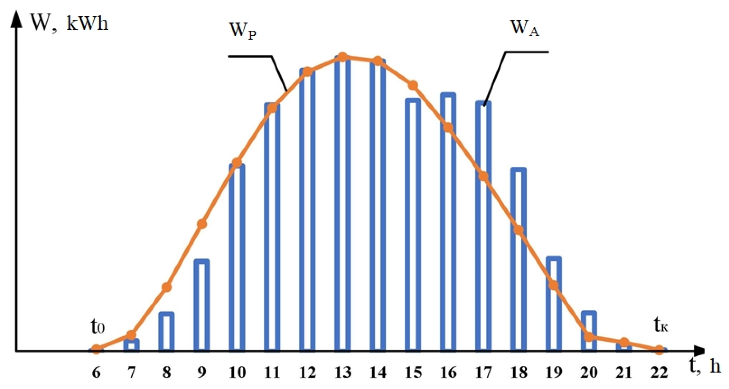
A peculiarity of RES operation in the EPS is its unstable generation. Moreover, due to the dependence on natural conditions during the day, its power varies over a fairly wide range—from zero to the set power. PVs generate power only during daylight hours and then according to an irregular schedule (see Figure 1). The power of wind turbines depends on the strength of the wind flow, which also changes all the time. Therefore, power and electricity losses that occur in electrical grids due to electricity flows from PV and wind turbines also change.

Losses of power in a given circuit (circuits) of the electric network due to the flow of RES electricity within it is determined using (9). For this, a vector is calculated, V_i, and a matrix of distribution loss, V, is determined, with the voltages in the nodes specified according to the power values in the same nodes of the grid, as well as the components of power losses:

$$\mathsf{\Delta }{\dot{\mathrm{S}}}_{\mathrm{bi}}={\dot{V}}_i\hspace{0.17em}{\dot{S}}_{\mathsf{\Sigma }}={\displaystyle \sum _{i\in {\theta }_L}{v}_i{s}_i}+{\displaystyle \sum _{j\in {\theta }_{RES}}{v}_j{s}_j},$$

(11)

where v—the elements of vector row ${\dot{V}}_i$; s—elements of the node power vector ${\dot{S}}_{\mathsf{\Sigma }}$; ${\theta }_L$ and ${\theta }_{RES}$—the arrays of node loads and RES, respectively.

A list of RES nodes ${\theta }_{RES}$ may consist of one or more nodes, depending on when losses in the line are determined from one RES or their group.

Electricity losses are the sum of power losses in all grid modes for the calculation period T:

$$\mathsf{\Delta }W={\displaystyle \underset{0}{\overset{T}{\int }}\mathsf{\Delta }P(t)dt} \mathrm{or} \mathsf{\Delta }W\approx {\displaystyle \sum _{i=1}^n\mathsf{\Delta }{P}_i\cdot }\mathsf{\Delta }{t}_i,$$

(12)

where $\mathsf{\Delta }P(t)$ represents the graph of changes in power loss over time T; $\mathsf{\Delta }{P}_i$—the power losses, which are assumed to be constant over time $\mathsf{\Delta }{t}_i$; n—the number of intervals into which the loss change schedule is divided $\mathsf{\Delta }P(t)$ (if $\mathsf{\Delta }{t}_i=\mathsf{\Delta }t=const$, then $n=T/\mathsf{\Delta }t$).

Which Formula (12) to use depends on the formulation of the problem and information support. We proceed from the fact that the task of balancing electricity in EPS modes for the next day is solved and telemetering is available at all nodes of electrical grids. In this case, the RES generation schedules are predicted and known ${\dot{S}}_{RES}(t)$, and according to the data of the automated system of commercial electricity accounting (ASCEA), the actual values of the produced RES electricity at time intervals are known $\mathsf{\Delta }t$.

The values of $\mathsf{\Delta }P(t)$ are determined according to the P(t) and Q(t) capacity forecast graphs in RES nodes. For example, for the i-th PV (see Figure 1),

$$\mathsf{\Delta }{W}_{RESi}^f={\displaystyle \underset{t_0}{\overset{t_k}{\int }}\mathsf{\Delta }{P}_{RESi}^f(t)}dt,$$

(13)

If we are referring to the RES group, then $\mathsf{\Delta }{W}_{RES}^f={\displaystyle \sum _{i\in \theta RES}\mathsf{\Delta }{W}_{RESi}^f}$.

The actual values of electricity losses for the same PV are defined as

$$\mathsf{\Delta }{W}_{RESi}^a={\displaystyle \sum _{i=1}^n\mathsf{\Delta }{P}_{RESi}^a\hspace{0.33em}}\mathsf{\Delta }t,$$

(14)

where $n=(t_k-t_0)/\mathsf{\Delta }t$.

The value of actual electricity losses of the RES group $\mathsf{\Delta }{W}_{RES}^a={\displaystyle \sum _{i\in {\theta }_{RES}}\mathsf{\Delta }{W}_{RESi}^a}$.

If the forecasted and actual values of electricity losses are brought to the same time period, then the error of forecasting electricity losses during balancing of the EPS mode is determined:

$$\delta ={\displaystyle \frac{\mathsf{\Delta }{W}_{RES}^f-\mathsf{\Delta }{W}_{RES}^f}{\mathsf{\Delta }{W}_{RES}^f}}100\%.$$

(15)

According to the value of the error δ, the power additional to the power of replacement of losses from RES by maneuverable EPS capacities or electricity storage is calculated [16,17,18].

4. Algorithm for Determining Power Flow and Energy Losses in Specified Branches of an Electric Grid

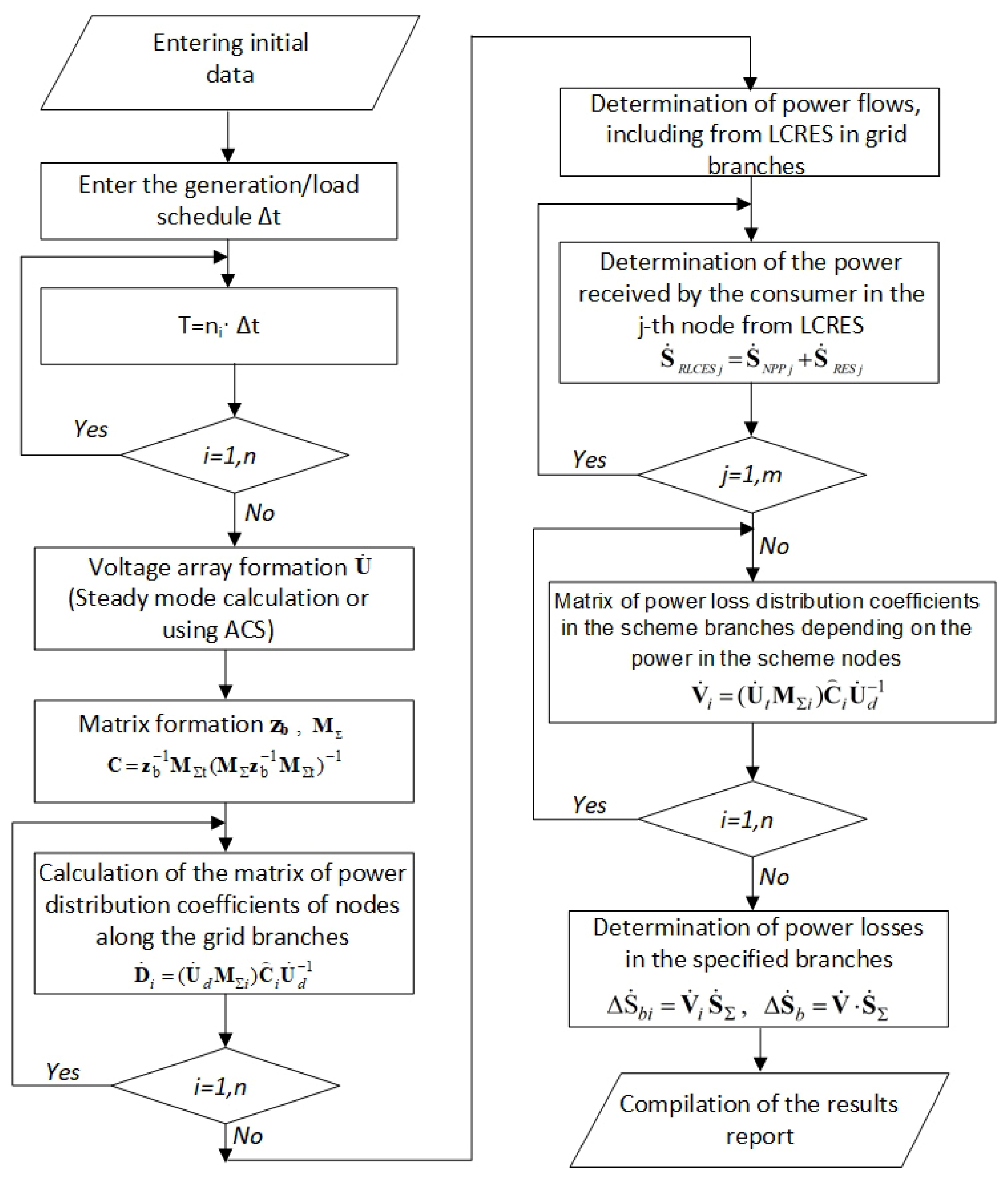
In Figure 2, the algorithm for determining the share of power generated by LCRES and delivered to a specified electricity consumer is presented. The approach embedded in the algorithm is based on identifying the power flows in the branches of the electric grid that are incident to the nodes containing the predefined list of electricity consumers supplied from LCRES. Directly at the node, using the power balance, the power consumed by each consumer specifically oriented toward consuming electricity from a particular LCRES is calculated with consideration of the physical processes occurring in the electric grid. Thus, it becomes possible to assess the amount of load coverage for a given consumer by LCRES that supply energy to the power system during a controlled time period T. The input data for the calculation include the parameters of the electric grid and node loads specified either as power values or load profiles, as well as the generation profiles of the low-carbon energy sources present in the grid.

To convert the consumer’s power demand into the amount of electricity consumed, methods of average or maximum loads are used. Depending on the selected method, either the average load ${\dot{S}}_{av}\hspace{0.17em}$ or the maximum load ${\dot{S}}_{max}\hspace{0.17em}$ of the consumer over period T is specified. A more accurate approach is to use a forecasted hourly consumption profile for the next day together with actual consumption data obtained from the automated control system (ACS). In the first case, the forecasted amount of electricity planned for consumption from LCRES is determined. In the second case, the actual amount of electricity consumed from LCRES is calculated.

These data are then transferred to the registry of Guarantees of Origin, taking into account the volume of guaranteed load coverage of the consumer with energy from low-carbon energy sources. Depending on the requirements and the technical capabilities of the metering system, the programme is launched either hourly or according to generation and consumption schedules within the electric grid.

The array of node voltages required for the calculations can be obtained in two ways: either as the result of steady-state grid operation analysis or from ACS measurements. If hourly forecasted values of LCRES generation and consumption are used, the voltages are determined from steady-state calculations or, when the required accuracy allows, from average statistical data. If the actual values are determined, the input data are the voltage measurements provided by the ACS.

In the algorithm shown in Figure 2, the matrix of the power-distribution coefficients of nodes across the branches of the electric grid D is determined from (1), taking into account expressions (4) and (5).

$${\dot{\mathrm{S}}}_b=({\dot{U}}_d{M}_{\mathsf{\Sigma }})\stackrel{⌢}{C}{\dot{U}}_d^{-1}\dot{S}=D \dot{S},$$

where $D=({\dot{U}}_d{M}_{\mathsf{\Sigma }})\stackrel{⌢}{C}{\dot{U}}_d^{-1}\hspace{0.33em}$.

After forming the array of node voltages, the incidence matrix $M_{\mathsf{\Sigma }}$ and the matrix of coefficients for the distribution of node-injected currents in the branches of the electric grid $\dot{C}$ are generated. The matrix of power-distribution coefficients for the nodes across the branches of the electric grid $\dot{D}$ is calculated. Using matrix $\dot{D}$, the portions of the total LCRES power ${\dot{S}}_{b\hspace{0.33em}LCRES}$ that flow through the branches of the grid are determined. Summing the LCRES power flows ${\dot{S}}_{b\hspace{0.33em}LCRES}$ in the branches incident to the j-th nodes with controlled consumption from LCRES makes it possible to determine the guaranteed volumes of electricity originating from LCRES for these consumers. Such nodes may be of two types. If a node is terminal, that is, only one branch carrying LCRES power ${\dot{S}}_{LCRES\hspace{0.17em}j}$ reaches it, then this power represents the amount of electricity originating from LCRES for the given consumer. The power ${\dot{S}}_{\hspace{0.17em}\hspace{0.17em}LCRES\hspace{0.17em}j}$ may be determined as the sum of the power flows from nuclear power plants ${\dot{S}}_{NPP\hspace{0.17em}j}$ and renewable sources ${\dot{S}}_{RES\hspace{0.17em}j}$ to the j-th node. In certain cases, depending on the topology, the operating mode of the electric grid, and the presence of distributed energy resources, the power ${\dot{S}}_{\hspace{0.17em}\hspace{0.17em}LCRES\hspace{0.17em}j}$ may be determined by only a single component—either from nuclear power plants or from renewable energy sources, respectively. If the node is an intermediate node, the power ${\dot{S}}_{LCRES\hspace{0.17em}j}$ is determined from the power balance at the j-th node.

Having determined the share of power from LCRES received by the consumer, it becomes possible and necessary to calculate the power losses caused by LCRES. In particular, responsibility for covering losses during transmission and distribution—within various settlement mechanisms—may be assigned either to the end consumer or to the producer (as in the case of PPA contracts). The matrix of power-loss distribution coefficients for each branch ${\dot{V}}_i$ is formed according to the grid topology defined in the input data. The energy losses in the specified branches and in the electric grid as a whole are determined using ${\dot{V}}_i$, and are also refined by actual node voltage values U and power values $\dot{S}$. Depending on the task formulation and input data, the “result protocol formation” stage converts the consumer’s LCRES-origin electricity and associated losses into the final reported values.

5. Algorithm for Determining the Dependence of Power Losses on PV Generation in Microgrids

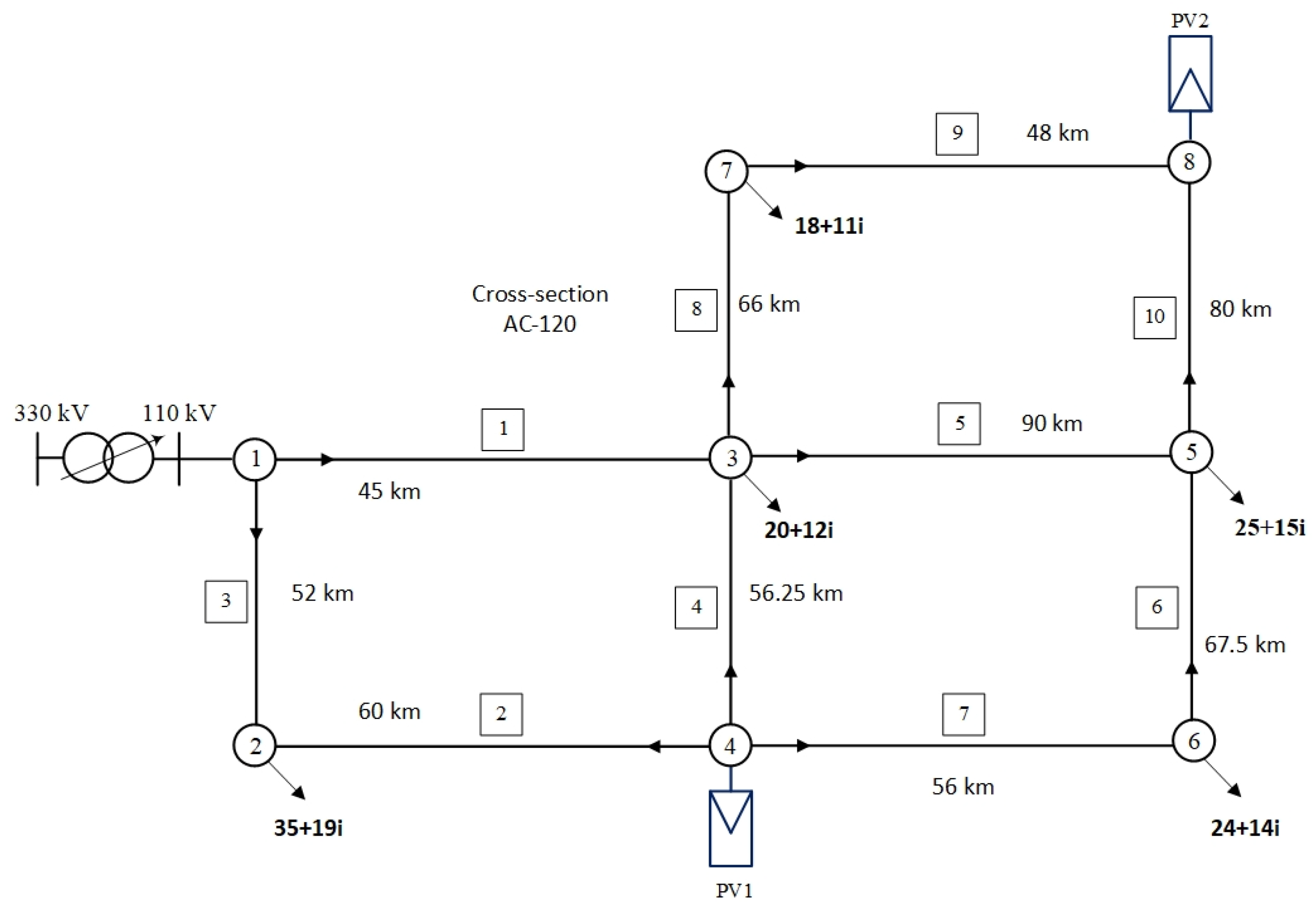
As an example, let us consider a fragment of a microgrid scheme. The parameters of the scheme are shown in Figure 3. The steady-state operation of the grid was calculated using the PowerFactory 15 software package. According to the variation in the generation output of photovoltaic power plants, the total active power losses were determined. The results are presented in

Table 1. Steady-state calculation results for different generation levels of PV1 and PV2.

PGEN PV1, MW	PGEN PV2, MW	ΔP, MW
1	29	8.29
5	25	8.21
7	23	8.19
9	21	8.18
11	19	8.19
13	17	8.21
15	15	8.25
17	13	8.3
19	11	8.36
21	9	8.44
23	7	8.54
25	5	8.65
27	3	8.79
29	1	8.91
1	15	9.83
3	15	9.58
5	15	9.33
7	15	9.10
9	15	8.87
11	15	8.66
13	15	8.45
15	15	8.25
17	15	8.06
19	15	7.87
21	15	7.7
23	15	7.53
25	15	7.37
27	15	7.22
29	15	7.07
15	1	10.36
15	3	10.00
15	5	9.66
15	7	9.34
15	9	9.04
15	11	8.76
15	13	8.49
15	15	8.25
15	17	8.02
15	19	7.8
15	21	7.6
15	23	7.42
15	25	7.26
15	27	7.1
15	29	6.97
0	0	12.59

.

The task is reduced to finding the optimal operating mode under which the power losses in the grid are minimized; that is, the objective function can be written as

$$\mathsf{\Delta }{P}_{MG}=f\hspace{0.17em}(P_{GEN PV1},P_{GENPV2})\to min,$$

(16)

where ΔP_MG denotes power losses in the microgrid (microgrid); P_{GEN PV1}, P_{GEN PV2}—generation power of PV1 and PV2, respectively.

According to the data in Table 1, the difference between the optimal and non-optimal operating modes may be approximately 9%.

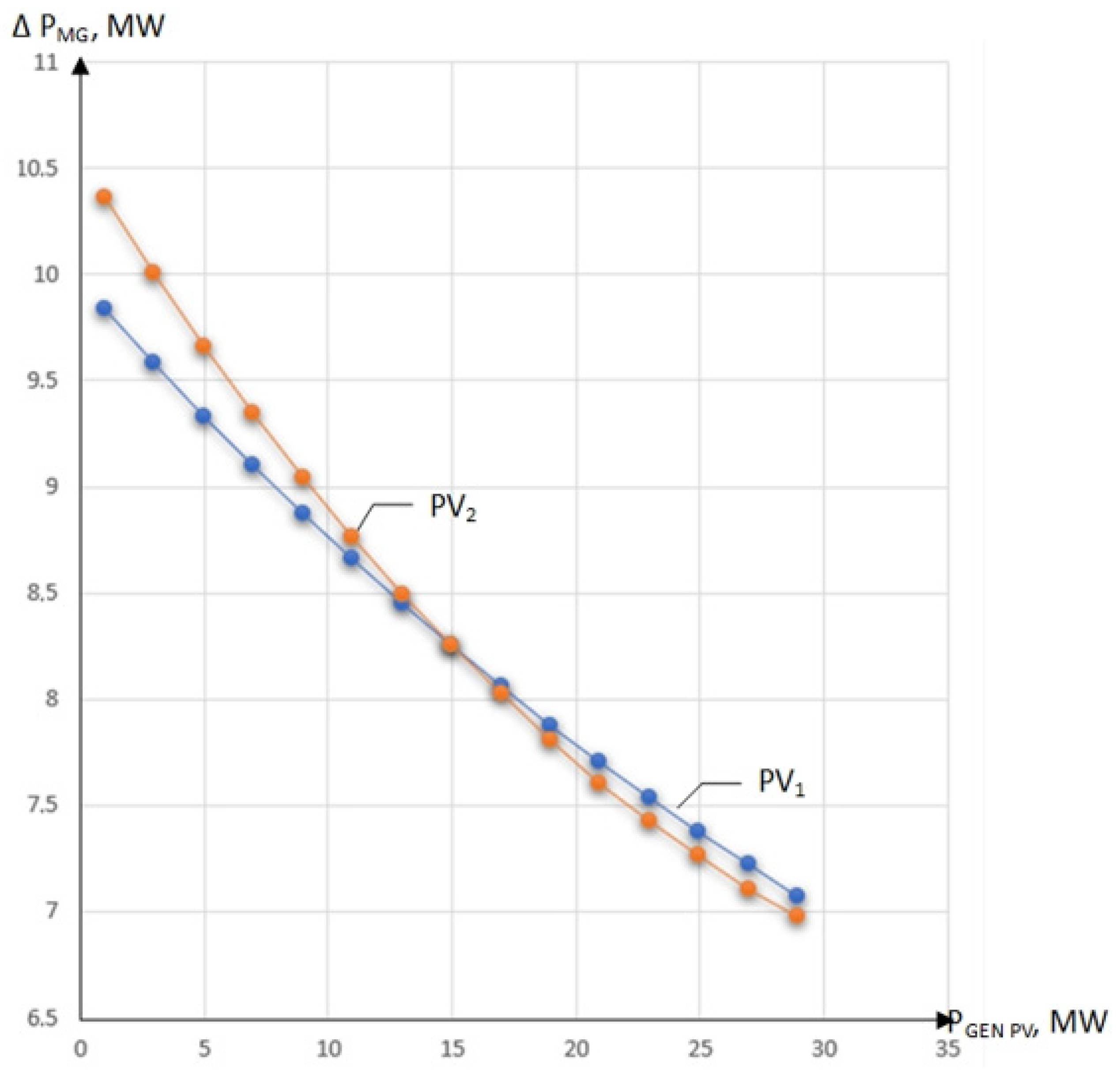
Let us present the obtained data in the form of graphical dependencies, as shown in Figure 4.

Let us determine the generation power values of PV1 and PV2 at which the power losses in the microgrid are minimized. For this purpose, we approximate the dependence $\mathsf{\Delta }P=f(P_{PV})$ using second-order polynomials:

$$\mathrm{for} \mathrm{PV}1—\mathsf{\Delta }P=0.001\cdot P_{GEN PV1}^2-0.1291\cdot P_{GEN PV1}+9.9548 \left(\mathrm{MW}\right),$$

(17)

with approximation accuracy R² = 0.9998;

$$\mathrm{for} \mathrm{PV}2—\mathsf{\Delta }P=0.0021\cdot P_{GEN PV2}^2-0.1844\cdot P_{GEN PV2}+10.533 \left(\mathrm{MW}\right),$$

(18)

with approximation accuracy R² = 1.

We set the first derivatives of these equations equal to zero:

$${\displaystyle \frac{d\mathsf{\Delta }P}{{\mathit{dP}}_{GEN PV1}}}=0.0002\cdot P_{GEN PV1}-0.1291\hspace{0.17em}\hspace{0.17em}=\hspace{0.17em}0,$$

$${\displaystyle \frac{d\mathsf{\Delta }P}{d{P}_{GEN PV2}}}=0.0042\cdot P_{GEN PV2}-0.1844\hspace{0.17em}\hspace{0.17em}=\hspace{0.17em}0.$$

If we consider the task of determining the parameters of the optimal operating mode from the perspective of increasing the installed generation capacity of the available photovoltaic power plants, then the minimum values of active power losses in the electric grid—ΔP = 5.79 MW—are achieved when the generated power of PV1 is P_{GEN PV1} = 64.55 MW, and the minimum values of active power losses in the grid ΔP = 6.485 MW are achieved when the generated power of PV2 is P_{GEN PV2} = 43.9 MW. These values are taken as baseline, since according to the similarity criterion, the dependence $\mathsf{\Delta }P=f(P_{PV})$ is approximated by a second-order polynomial. With both stations disconnected, the power losses in the grid amount to 12.59 MW.

The analytical dependencies of active power losses in the electric grid on the generated PV power, expressed in per-unit form, were obtained as a second-order polynomial using the nonlinear regression algorithm based on the Levenberg–Marquardt method and central difference technique in the CurveExpert Basic 2.2.3 software environment.

As a result of polynomial approximation of the data from

Table 2. Per-unit generated PV power and power losses.

PGEN PV1, MW	p.u.	PGEN PV2, MW	p.u.	ΔP, MW	p.u
1	0.015	15	-	9.83	1.698
3	0.046	15	-	9.58	1.655
5	0.077	15	-	9.33	1.611
7	0.108	15	-	9.10	1.572
9	0.139	15	-	8.87	1.532
11	0.170	15	-	8.66	1.496
13	0.201	15	-	8.45	1.459
15	0.232	15	-	8.25	1.425
17	0.263	15	-	8.06	1.392
19	0.294	15	-	7.87	1.359
21	0.325	15	-	7.7	1.330
23	0.356	15	-	7.53	1.301
25	0.387	15	-	7.37	1.273
27	0.418	15	-	7.22	1.247
29	0.449	15	-	7.07	1.221
15	-	1	0.023	10.36	1.598
15	-	3	0.068	10.00	1.542
15	-	5	0.114	9.66	1.490
15	-	7	0.159	9.34	1.440
15	-	9	0.205	9.04	1.394
15	-	11	0.251	8.76	1.351
15	-	13	0.296	8.49	1.309
15	-	15	0.342	8.25	1.272
15	-	17	0.387	8.02	1.237
15	-	19	0.433	7.8	1.203
15	-	21	0.478	7.6	1.172
15	-	23	0.524	7.42	1.144
15	-	25	0.569	7.26	1.120
15	-	27	0.615	7.1	1.095
15	-	29	0.661	6.97	1.075

, we obtain the equation for the per-unit power losses in the grid for PV1:

$$\mathsf{\Delta }{P}_{*}=\hspace{0.17em}0.971\cdot P_{*GEN PV1}^{-0.246}+ 0.056\cdot P_{*GEN PV1}^4,$$

(19)

where $P_{GEN PV1}^{*}=P_{GEN PV1}/P_{GEN PV1}^{opt}\hspace{0.17em}$—generated PV1 power in per-unit values.

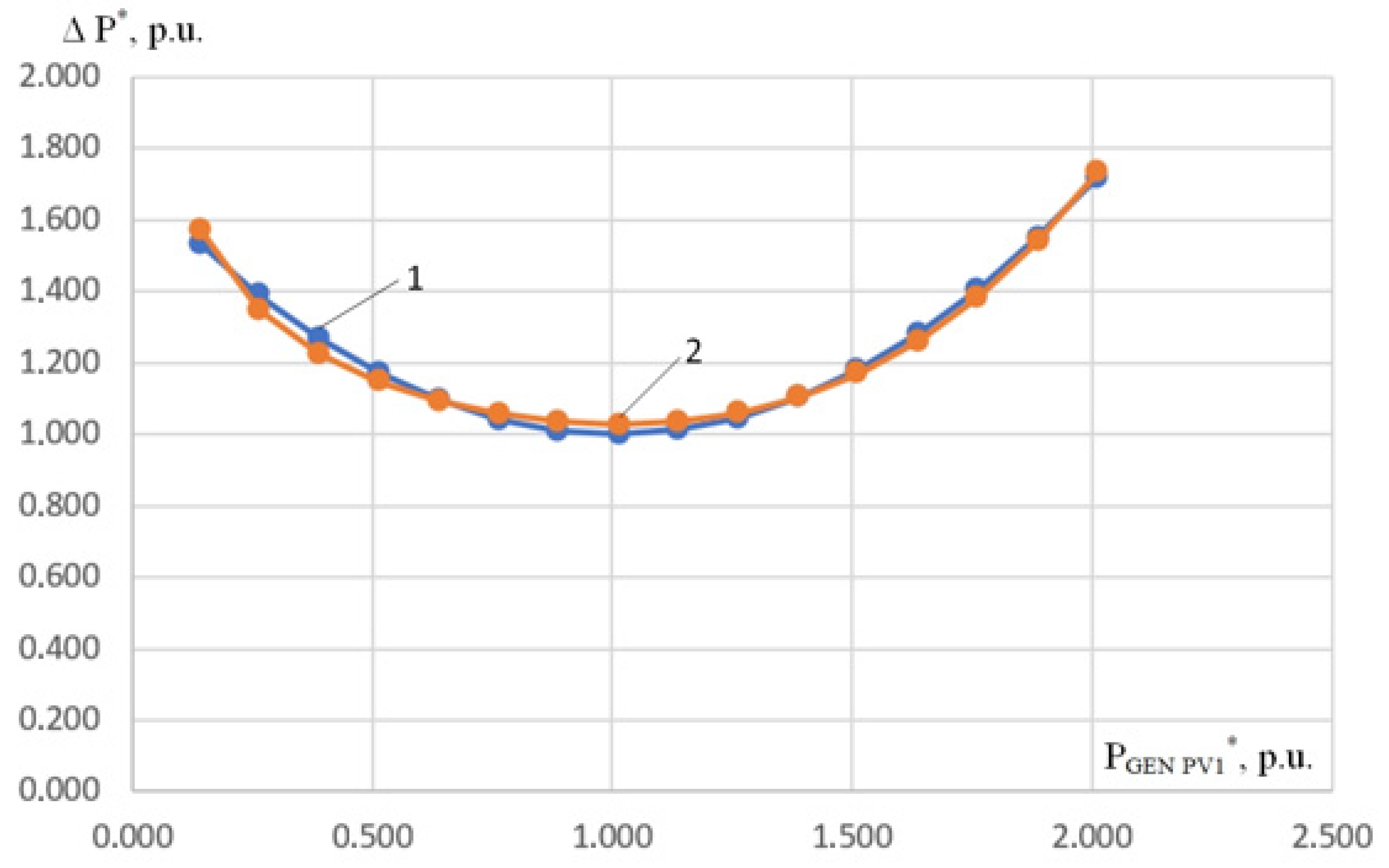
Within the range of variation in the generated PV1 power from 0.14 to 2.01 p.u., the approximation produced the following results: approximation error—0.029 p.u., correlation coefficient—0.987 p.u.

Figure 5 shows the plots of the dependence of the per-unit values of the function $\mathsf{\Delta }P=f(P_{PV1})$ on the per-unit values of the generated PV1 power.

Similarly, the following dependencies were obtained for PV2:

$$\mathsf{\Delta }{P}_{*}=\hspace{0.17em}0.929\cdot P_{*\mathrm{GEN} \mathrm{PV}2}^{-0.201}+0.1\cdot P_{*\mathrm{GEN} \mathrm{PV}2}^3$$

(20)

where P_{*GEN PV2}—generated PV2 power in per-unit values.

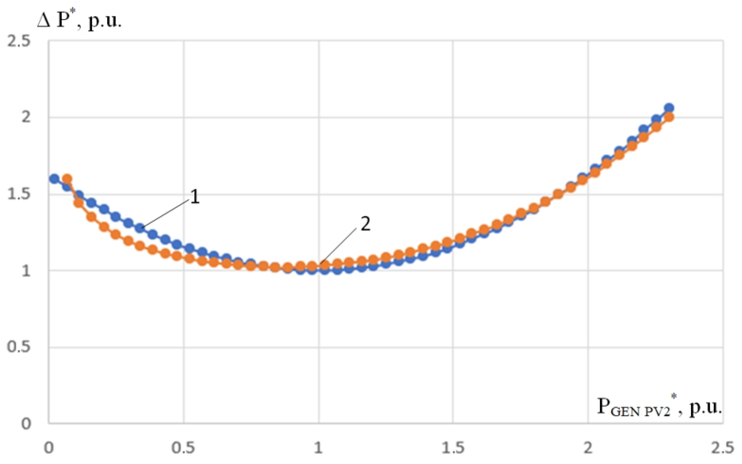
Within the range of variation in the generated PV2 power from 0.02 to 2.3 p.u., the approximation yielded the following results: approximation error—0.057 p.u., correlation coefficient—0.9863 p.u.

Figure 6 shows the plots of the dependence of the per-unit values of the function $\mathsf{\Delta }P=f(P_{PV1})$ on the per-unit values of the generated PV2 power. The dependencies of the objective function values on the generated PV2 power constructed using CurveExpert are shown in Figure 6.

The approximated dependencies (1) and (2) (see Figure 6) represent the criterion-based models of the process of adjusting the power outputs of PV1 and PV2 to influence the power flows in the microgrid with the aim of reducing losses, optimizing the operating mode, and improving the operational efficiency of such plants. The coefficients of the terms in these dependencies are normalized to unity (within approximation accuracy) and serve as similarity criteria [19,20].

Determining the Optimality Range and Limit Values of the Insensitivity Range

Now, let us apply the method to determine the optimality ranges and the limit values of the insensitivity ranges for the ACS of PV1 and PV2. We assume an allowable deviation of the power losses from their optimal value of 5%.

The problem of optimal control of the PV1 or PV2 generation power in terms of minimizing microgrid power losses is expressed through the following objective functions:

$$\mathsf{\Delta }{P}_{\ast \mathrm{M}\mathrm{G}}=\hspace{0.17em}\hspace{0.17em}0.971\cdot P_{\ast \mathrm{GEN} \mathrm{PV}1}^{-0.246}+0.056\cdot \hspace{0.17em}{P}_{\ast \mathrm{GEN}\hspace{0.17em}\mathrm{PV}1}^4\hspace{0.17em}\to \hspace{0.17em}min,$$

(21)

$$\mathsf{\Delta }{P}_{\ast \mathrm{MG}}=\hspace{0.17em}0.929\cdot P_{\ast \mathrm{GEN} \hspace{0.17em}\mathrm{PV}2}^{-0.201}+0.1\cdot \hspace{0.17em}{P}_{\ast \mathrm{GEN} \hspace{0.17em}\mathrm{PV}2}^3\hspace{0.17em}\hspace{0.17em}\to \hspace{0.17em}min$$

(22)

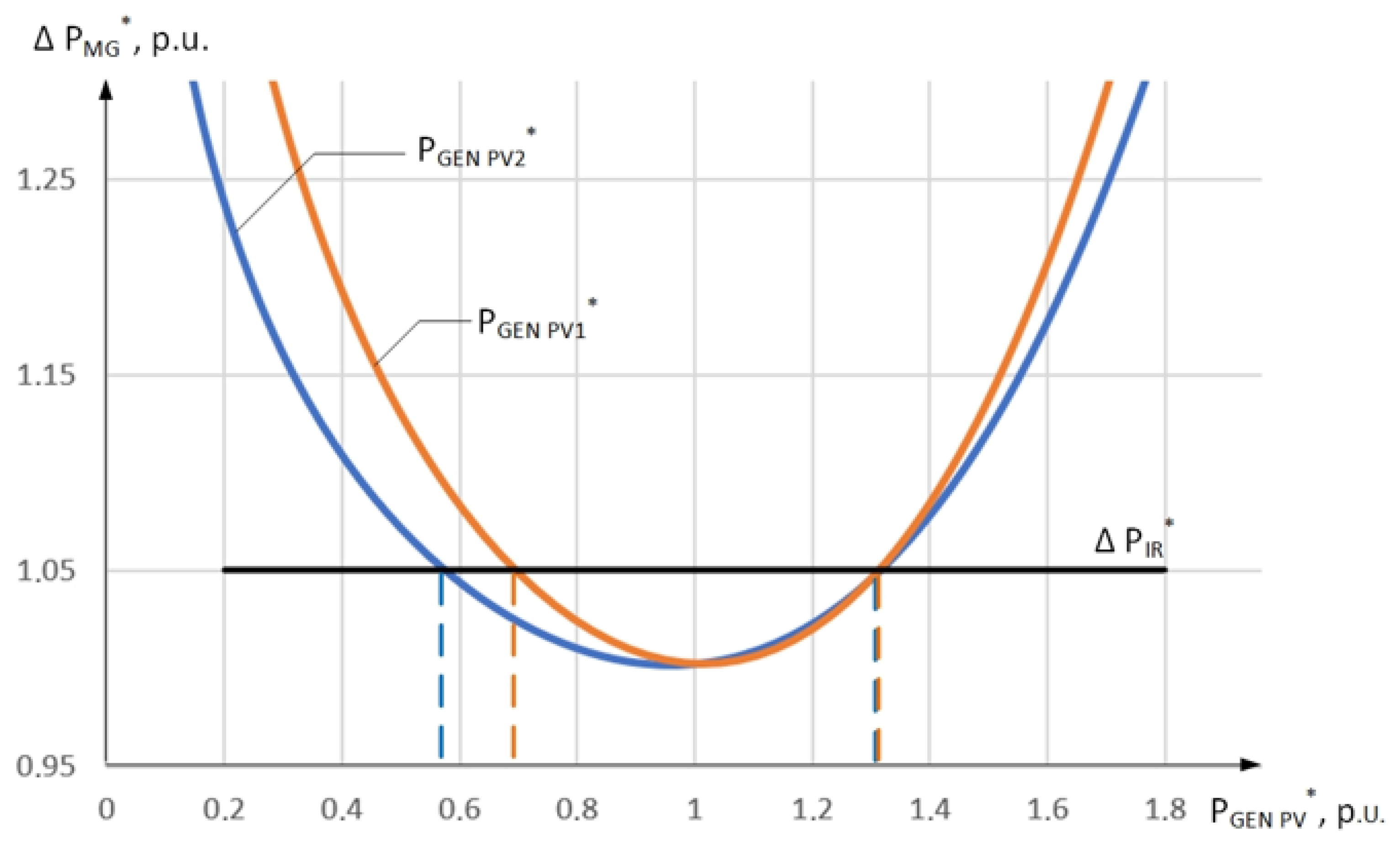
Using the graph-analytical method, we determine the limits of the optimality range for the generation of PV1 and PV2 in per-unit values, as shown in Figure 7. Accordingly, the limit values of the insensitivity range for the ACS of PV1 are taken as 0.58–1.3 and for the ACS of PV2 as 0.68–1.3. The calculation results for the PV plants are summarized in

Table 3. Optimality ranges of PV generation power.

PV	P−*. r.u.	P+*. r.u.	ΔP−*. r.u.	ΔP+*. r.u.	ΔP−. MW	ΔP+. MW
PV1	0.58	1.3	0.42	0.3	27.1	58.1
PV2	0.68	1.3	0.32	0.3	14.05	13.17

.

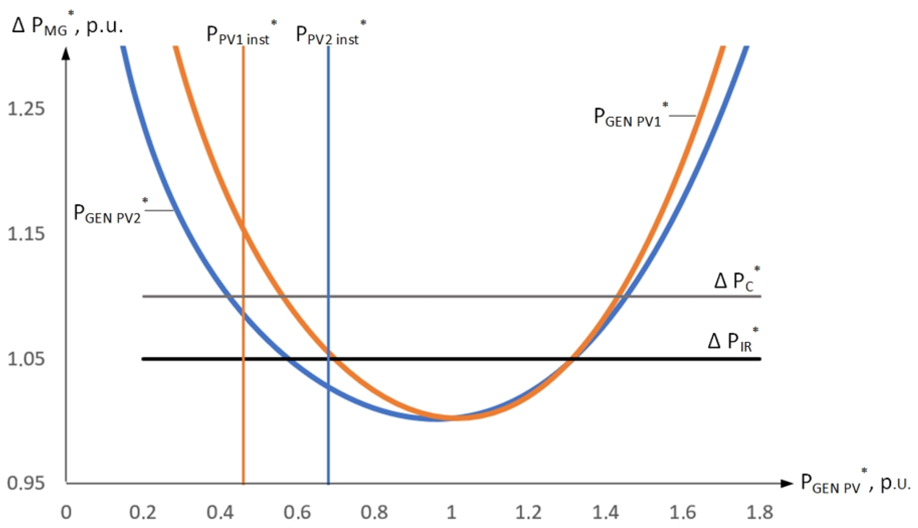
The tolerances determined in this way reflect the actual capability of the PV plants to influence the microgrid operating-mode optimization process. As can be seen from Figure 7, the dependence of the per-unit active power losses in the microgrid on the generated power is steeper for the first PV plant than for the second one. Moreover, Figure 8 shows that in the current operating mode of the microgrid, when the grid losses amount to 1.07 p.u., the generated power of PV2 falls within the insensitivity range. Consequently, at this moment, adjusting the operating mode using this plant is impractical.

At the same time, increasing the generated power of PV1 makes it possible to change the operating mode of the microgrid and reduce its power losses. If both PV plants begin operating within their insensitivity ranges, then for a certain period, the variations in the daily microgrid load profile and PV generation will not require additional control actions. However, the generated power of a PV plant is limited by its installed capacity.

In Figure 8 (for the case of significantly reduced node load), the installed capacity of PV1 is shown by the orange line, and the installed capacity of PV2 by the blue line.

As can be seen from Figure 8, from the perspective of optimal control, it is advisable to adjust the generation power of PV2, because its installed capacity allows it to enter the insensitivity range. In contrast, increasing the generation power of PV1 up to its installed capacity does not allow it to enter the insensitivity range. Therefore, for the current operating mode of the microgrid, increasing the generation power of PV1 is impractical.

6. Conclusions

In modern power supply systems, the problem arises of determining the amount of “clean” electricity consumed, namely, electricity originating from low-carbon and renewable energy sources, including wind power plants and photovoltaic power plants. Since public electric grids are used to transmit electricity to consumers, it is essential for consumers to receive guaranteed confirmation that the electricity they consume indeed originates from LCRES.

The complexity of this task lies in its nonlinear nature, which makes it impossible to directly apply the transposition method to its solution. In this work, a method is proposed for determining the origin of electricity consumed by individual users, attributed to specific LCRES units. The method is based on forming a matrix of power-distribution coefficients that allocates the contributions of LCRES generating nodes across the branches of the electric grid incident to the consumer node.

The matrix of branch power-distribution coefficients depends on the grid parameters, which, under certain assumptions, are considered constant, and on the node voltage values, which are determined by the prevailing generation and load at the corresponding nodes. The nonlinear dependence of the consumed power at the nodes including the portion attributed to LCRES on the operating parameters is preserved through simultaneous measurement or steady-state calculation of the generation and load values, as well as the associated node voltages. Determining the distribution coefficients using current node voltages effectively corresponds to transitioning to a linearized model of the normal operating mode of the electric grid with fixed node powers and voltages.

In determining the amount of “clean” electricity consumed by end users, it is also necessary to assess the electricity losses caused by the transfer of power from LCRES. To address this problem, this article additionally proposes a matrix-based method for determining the power losses induced by renewable and low-carbon energy sources in electric grids. The method employs a mathematical model and steady-state power flow analysis to determine the matrix of power-loss distribution coefficients. By taking into account the time-varying output of weather-dependent generating units and the stable generation of nuclear power plants, the method enables the calculation of both instantaneous and cumulative energy losses over specified time intervals.

The method described can serve as a tool for confirming the Guarantees of Origin of energy consumed from a public electric grid and for determining the share of LCRES power in the power flows delivered to consumers. This enhances transparency in the functioning of the electricity market and supports the development of low-carbon generation. The method allows for the influence of LCRES on the operating parameters of the electric power system to be taken into account and can be used in operational electricity balance planning. The effectiveness of the method is demonstrated through specific case studies. The results obtained using the matrix method were compared with the outcomes of computer simulations performed in the PowerFactory software.