Single-Attention Large Language Model for Efficient Multi-Regional Electricity Demand and Generation Forecasting

Abstract

Electricity forecasting is one of the most crucial aspects in maintaining stable, reliable, and autonomous power systems. While recently developed forecasting methods based on large language models can make accurate predictions, these models are still struggling due to their computational complexity, which requires more computing power, and their reliance on carefully designed prompts. This makes them complicated and harder to use in practice. To address this, we propose a Single-Attention Large Language Model (SA-LLM) that uses a unified attention mechanism to understand relationships between main and additional variables, without the need for manually created prompts. The proposed framework has been tested on real electricity supply and demand datasets, which are obtained from major U.S. electricity markets, including PJM, MISO, NYISO, ISO New England, ERCOT, SPP, and CAISO. Experimental results demonstrate that the proposed SA-LLM method outperforms the existing counterpart methods in terms of accuracy and associated errors. More specifically, the SA-LLM has also achieved a 22.5% improvement in the mean absolute error compared with traditional LSTM-based models, while reducing memory usage by 52.1% and training time by 38.4% relative to recent LLM-based methods. Furthermore, the SA-LLM demonstrates strong zero-shot generalization, achieving an additional 18.2% improvement in the MAE on previously unseen regions.

1. Background

Currently, the world has experienced an unprecedented increase in electricity consumption driven by urbanization, industrialization, and digitization. This increased energy demand has placed immense pressure on energy producers to meet sustainability and resilience goals [1,2]. The sense of urgency arising from the need to reduce climate change has further intensified efforts to reduce carbon emissions and shift towards a low-carbon energy system [3,4]. However, these goals cannot be accomplished merely by investing in infrastructure for renewable resources. They demand smarter management systems that are adaptable, data-driven, and equipped with real-time processing to dynamically optimize their functions. The concept of the smart grid has become increasingly significant in this process because it offers an effective way to coordinate and optimize distributed energy resources (DERs) [5,6]. Accurate forecasting methods for electricity demand and renewable power generation are very important to ensure the efficiency and stability of the smart power grid [7,8]. In practice, inaccurate forecasts can lead to financial losses and prediction errors. Traditional forecasting methods have been widely used and provide good results, including models such as LSTM, ARIMA, and SVR. However, these models often struggle to capture the uncertainty and complexity of modern power systems [9]. The modern power networks are being influenced by various dynamic and uncertain factors, such as renewable energy generation, weather variations, and market trends, many of which behave nonlinearly. As a result, the energy market has shifted toward using advanced AI models, especially DL techniques that can uncover complex patterns in data. LLMs have shown promise in this area because their attention mechanisms can theoretically capture long-term dependencies across multiple data series. However, their application in energy modeling has been limited due to challenges in effective cross-series learning and their reliance on manually designed prompts [10].

1.1. Electricity Forecasting

Electricity load forecasting has advanced significantly over the years and encompasses a range of techniques, from classical statistical methods to advanced machine learning and deep learning approaches [11]. Classical statistical techniques such as ARIMA and exponential smoothing have been widely adopted due to their simplicity and ease of interpretation. Yet, when it comes to the nonlinearity present in contemporary energy infrastructure, their effectiveness remains questionable, as they essentially belong to the class of linear modeling techniques [12]. ML algorithms, including support vector machines (SVMs) and random forests (RFs), have been investigated for their ability to model nonlinear relationships [13]. Although ML techniques are highly useful, they often require extensive feature engineering, which can be problematic when generalization to unseen conditions is required [14]. Recently, the DL approach has shown impressive results in EFP applications because it can automatically extract relevant features from data [15]. Among DL models, ANNs, RNNs, and, more specifically, LSTMs have proven successful in extracting complex time-related features from energy data [16,17]. Recently, hybrid deep learning models have emerged that combine recurrent or convolutional structures with attention networks to promote interpretability and model long-term dependencies in time-series data [18,19]. Advances in transformer-based models, including Informer and Autoformer, have further improved time-series forecasting, yielding greater efficiency and higher accuracy for long-horizon forecasting. Recent improvements have made smart grid forecasting systems smarter [20,21,22,23,24,25,26,27]. People now use machine learning and transformer models instead of old statistical methods. These new methods can predict energy use more accurately. It is also important that these models are easy to understand and can work well in different situations and times.

1.2. LLMs for Forecasting

LLMs have been widely studied for their ability to support advances across different domains [28,29]. Their large number of parameters allows them to process and learn from large datasets [30]. Moreover, traditional AI and machine learning models often find it difficult to handle relationships between internal and external variables in the dataset [31]. LLMs are also applied in areas beyond text generation [32]. LLMs have recently been used for both short- and long-term forecasting because they can capture important relationships and handle different types of uncertainties and correlations [32]. Models like ARIMA and deep learning often have difficulty handling relationships caused by external or internal variables in the datasets [31]. This limitation exists because LLMs use parallel processing, which allows them to handle longer sequences more efficiently than traditional deep learning models [33]. As a result, many transformer-based time-series approaches have shown better performance than classical forecasting methods in various applications. Forecasting algorithms can generally be grouped into two main types. The first type involves reprogramming pre-trained LLMs by adding instructional information to the original time-series data to guide the forecasting process [34,35,36]. The second category focuses on fine-tuning the model with time-series data. In some cases, it uses multi-stage pipelines and contrastive learning to help the model better understand patterns over time [37].

2. Contribution

Accurate electricity forecasting is very important for planning and running modern smart power grids. LLMs are effective at analysis, but they are not very effective at predicting time-based data because they often miss temporal patterns and require complex prompt setups. We propose an SA-LLM that uses a single-attention mechanism to capture both temporal changes and relationships among features. We tested it on real electricity demand and supply data from major U.S. markets: PJM, MISO, NYISO, ISO New England, ERCOT, SPP, and CAISO. Following prior work, we highlight the key gaps and our primary contributions. Nevertheless, we identify significant challenges on the horizon for LLM-based forecasting.

1.

Fine-tuning difficulty: Since a lot of optimization is done for pre-trained LLMs, naive fine-tuning often results in negligible improvements or even leads to overfitting issues. In addition, because LLMs have highly complex architectures, it is difficult to determine which components need to be fine-tuned [6].

2.

Prompt design limitations: Prompt engineering has been used as a means of improving LLM performance for natural language processing. However, prompt engineering for time-series forecasting is challenging due to the complex temporal dependencies and the large number of features.

3.

Regional variability: It is observed that there are differences between countries with respect to geography when it comes to climate, electricity demand, and renewable energy generation. These differences make it difficult to identify universal models, and only a limited number of studies are conducted.

Key Contributions

• We introduce the SA-LLM, a new time-series forecasting framework that employs a single-attention mechanism to learn from target variables, yet requires manual prompt tuning.
• We provide a Graph Neural Network (GNN) module to capture spatial and inter-regional relationships, improving forecasting accuracy.
• We evaluate the SA-LLM across major U.S. electricity markets, showing it outperforms LSTM and previous LLM models, reducing the MAE by 22.5%, memory usage by 52.1%, and training time by 38.4%.
• We evaluate the SA-LLM in zero-shot scenarios and find that it reduces the MAE by 18.2% on unseen regions, demonstrating strong generalization across different locations and times.
• We offer a unified approach to spatio-temporal electricity forecasting that combines LLM-based feature extraction with optional graph-based spatial modeling.

3. Methodology

In time-series forecasting, two widely used mainstream strategies are employed [38,39]. Theoretically, this strategy offers higher modeling capacity since it learns complex inter-variable relationships. On the other hand, the CI strategy is more robust to noise and generalizes better since it focuses on self-correlations within each channel [39]. In practice, forecasting tasks typically consider multiple variables, such as predicting electricity demand and generation from historical power and weather data. Unlike full-variable and single-variable forecasting, the former benefits more from capturing inter-variable relationships, without the need to predict all variables. Unfortunately, LLMs face challenges in adopting channel-independent training strategies [40,41], in which a model computes the loss for all variables even though only a subset is required for prediction. Another challenge is that of prompt engineering. Approaches such as Tempo, which employs semi-soft prompts combining both hard and soft vectors, or TimeLLM, which appends the prompt as an input prefix, require careful task-specific tuning [34,41]. The need to fine-tune LLMs for each task makes them more complex and harder to use across different time-series forecasting problems.

3.1. Mainstream Strategies for Time-Series Forecasting

Two popular mainstream strategies are widely used [39]. These strategies are described mathematically as follows:

• Model-Based Optimization (Attention-Enhanced LLM) [39]

Let ${\mathbf{X}}_t\in {\mathbb{R}}^d$ denote the input features at time step t, and ${\mathbf{y}}_t\in \mathbb{R}$ denote the target variable. The model-based strategy constructs a predictive mapping $f_{\theta }$ parameterized by $\theta$ as presented in (1):

$${\widehat{\mathbf{y}}}_t=f_{\theta }\left({\mathbf{X}}_t\right)=\mathrm{Attention}({\mathbf{X}}_t;{\theta }_{\mathrm{att}})+g_{\varphi }\left({\mathbf{X}}_t\right),$$

(1)

where $\mathrm{Attention}({\mathbf{X}}_t;{\theta }_{\mathrm{att}})$ emphasizes critical temporal patterns, $g_{\varphi }\left({\mathbf{X}}_t\right)$ extracts local features, and $\theta =\{{\theta }_{\mathrm{att}},\varphi \}$ are learnable parameters. The model minimizes the mean squared error with regularization as in (2):

$${\mathcal{L}}_{\mathrm{MSE}}={\displaystyle \frac{1}{T}}\sum _{t=1}^T\parallel {\mathbf{y}}_t-{\widehat{\mathbf{y}}}_t{\parallel }_2^2+\lambda {\parallel \theta \parallel }_2^2.$$

(2)

2.

Model-Free Reinforcement Learning (TimeLLM) [41]

For comparative purposes, define the system state ${\mathbf{s}}_t\in \mathcal{S}$ and action ${\mathbf{a}}_t\in \mathcal{A}$. The environment provides a reward $r_t$ based on prediction accuracy. The objective of the model-free RL strategy is to learn a policy ${\pi }_{\theta }:\mathcal{S}\to \mathcal{A}$ that maximizes the expected cumulative reward in Equation (3):

$$J\left(\theta \right)={\mathbb{E}}_{{\pi }_{\theta }}\left[\sum _{t=0}^T{\gamma }^t{r}_t({\mathbf{s}}_t,{\mathbf{a}}_t)\right],$$

(3)

where $\gamma \in [0,1]$ is the discount factor. The policy is updated via Proximal Policy Optimization (PPO) in Equation (4):

$$\theta \leftarrow \theta +\alpha {\widehat{\mathbb{E}}}_t\left[{\displaystyle \frac{{\pi }_{\theta }\left({\mathbf{a}}_t\right|{\mathbf{s}}_t)}{{\pi }_{{\theta }_{\mathrm{old}}}\left({\mathbf{a}}_t\right|{\mathbf{s}}_t)}}{\widehat{A}}_t\right],$$

(4)

where ${\widehat{A}}_t$ is the advantage estimate, and $\alpha$ is the learning rate. Equations (1) and (2) formalize the model-based LLM strategy used in the SA-LLM, while Equations (3) and (4) describe the model-free RL (TimeLLM) for reference only.

3.2. Motivation for a Unified Attention Mechanism

The SA-LLM architecture is based on a unified attention mechanism that jointly models temporal and cross-variable dependencies in a multivariate time series. The input sequence is defined in Equation (5) as

$$\mathbf{X}=\{{\mathbf{x}}_t\in {\mathbb{R}}^V\mid t=1,\dots ,T\},$$

(5)

and the forecasting task requires learning mappings of the form shown in Equation (6):

$$\left(x_t^i\right)⟶\left(x_{t^{\prime }}^j\right),\forall t,t^{\prime }\in \{1,\dots ,T\},i,j\in \{1,\dots ,V\}.$$

(6)

To model these dependencies, the SA-LLM constructs token representations by combining temporal and variable embeddings, as defined in Equation (7):

$${\mathbf{h}}_t^i={\mathbf{W}}_x{x}_t^i+{\mathbf{E}}_t+{\mathbf{E}}_i.$$

(7)

These representations are processed by the unified attention mechanism. The attention matrix is computed using the formulation in Equation (8):

$$A=\mathrm{softmax}\left({\displaystyle \frac{Q{K}^{\top }}{\sqrt{d}}}\right),$$

(8)

where the projections Q, K, and V follow Equation (9):

$$Q=H{W}_Q,K=H{W}_K,V=H{W}_V.$$

(9)

Since the representation H in Equation (7) combines both temporal and variable information, each attention coefficient depends on these components jointly, as expressed in Equation (10):

$$A_{ij}=g(t_i,t_j,v_i,v_j,x_i,x_j).$$

(10)

3.3. Proposed Single-Attention LLM

Existing CI and CD time-series models are typically complex and require extensive tuning. However, the proposed SA-LLM model simplifies this by using a single-attention mechanism that captures the behavior of different variables and their interactions with one another, without compromising its predictive power or ability to curb overfitting. In contrast to traditional CI approaches, which neglect target and context interactions, and CD approaches, which are typically underpinned by computationally intensive joint modeling of entire channels, the SA-LLM introduces a hybrid model. Instead of learning target self-correlations and dependencies among multiple variables, as expressed by auxiliary features, the SA-LLM employs a unified attention block prior to LLM inference. As such, targeting and efficient aggregation become feasible, eliminating computations related to non-target variables and capturing essential dependencies to ensure an accurate time-series forecast. The SA-LLM architecture is composed of six tightly coupled modules, each designed to address a specific modeling bottleneck.

3.3.1. Word Projection Layer

Although LLMs are used, the vocabularies are optimized for language semantics, which is highly redundant for time-series tasks. The SA-LLM uses a projection layer that maps the LLM embedding to a smaller task-specific embedding. If the embedding size of the vocabulary is $D_{orig}$, and the projected size $D_{proj}$ is set to 2000 in this work, then the projection is done by the following Equation (11):

$${\mathbf{E}}_{proj}={\mathbf{E}}_{orig}{\mathbf{W}}_{proj},{\mathbf{W}}_{proj}\in {\mathbb{R}}^{D_{orig}\times D_{proj}},$$

(11)

where ${\mathbf{E}}_{orig}$ represents the original embeddings and ${\mathbf{E}}_{proj}$ represents the projected embeddings. This operation focuses the LLM input representation on the relevant structural features of the domain, improving convergence stability and computational efficiency. Equation (11) shows how the initial high-dimensional embeddings are linearly projected into a lower-dimensional space.

3.3.2. Single Unified Attention Module

The SA-LLM model computes the query, key, and value projections from the input feature matrix $\mathbf{F}\in {\mathbb{R}}^{T\times C}$, where T denotes the sequence length, and C represents the number of features. The linear projections are defined as in Equation (12):

$$\mathbf{Q}=\mathbf{F}{\mathbf{W}}_q,\mathbf{K}=\mathbf{F}{\mathbf{W}}_k,\mathbf{V}=\mathbf{F}{\mathbf{W}}_v,$$

(12)

where ${\mathbf{W}}_q,{\mathbf{W}}_k,{\mathbf{W}}_v\in {\mathbb{R}}^{C\times d_h}$ are learnable weight matrices, and $d_h$ denotes the attention head dimension. The attention weights are computed using the scaled dot-product attention mechanism presented in Equation (13):

$$\mathbf{A}=\mathrm{Softmax}\left({\displaystyle \frac{\mathbf{Q}{\mathbf{K}}^{\top }}{\sqrt{d_h}}}\right).$$

(13)

The attention-enhanced representation is then obtained as in Equation (14):

$$\mathbf{Z}=\mathbf{A}\mathbf{V},$$

(14)

where $\mathbf{A}\in {\mathbb{R}}^{T\times T}$ contains normalized attention coefficients. The scaling factor $\sqrt{d_h}$ ensures numerical stability prior to the Softmax operation. This unified attention mechanism enables each feature to attend to its own historical patterns as well as correlated features, thereby jointly modeling temporal and cross-feature dependencies.

3.3.3. Frozen Pre-Trained LLM Backbone

The attention-enhanced embeddings ${\mathbf{X}}_{attn}$ are combined with positional encodings $\mathbf{PE}$ and input to a frozen pre-trained LLM with N transformer layers:

$${\mathbf{H}}_{LLM}=\mathrm{LLM}({\mathbf{X}}_{attn}+\mathbf{PE}),$$

(15)

where ${\mathbf{H}}_{\mathrm{LLM}}$ are the output embeddings. Freezing the LLM preserves its pre-trained representations, prevents forgetting, and reduces computational cost, thereby treating it as a high-capacity temporal feature transformer.

3.3.4. Auxiliary Feature Extractor

This module captures general patterns and hidden relationships among non-target variables. Instead of using complex recurrent or attention-based encoders, we apply a simple linear transformation:

$$H_{\mathrm{aux}}=X_{\mathrm{nt}}{W}_f+b_f,$$

(16)

where $X_{\mathrm{nt}}$ are the non-target features, $W_f$ is a learnable weight matrix, and $b_f$ is a bias. This embedding adds context, improving prediction accuracy and stability.

3.3.5. Frozen LLM Backbone: Benefits and Limitations

The LLM backbone is kept frozen in order to avoid forgetting the pre-trained knowledge and minimize the computational and memory requirements. The added layers in the model are used for numerical time-series tasks. These layers act as adapters for the LLM backbone. These layers map the structured input data into the LLM’s representation space. The backbone is frozen in the model. Therefore, the model cannot adapt to domain-specific numerical data. As a result, the model’s performance degrades when the task data differ significantly from the pretraining data.

3.3.6. Attention-Based Feature Fusion and Feedforward Refinement:

Embeddings from the LLM, $E_{\mathrm{LLM}}$, are combined with auxiliary embeddings, $E_{\mathrm{aux}}$, via concatenation to create a joint representation, which is then processed by a shared attention mechanism (Equation (17)):

$$Z_{\mathrm{fusion}}=\mathrm{Attention}\left([E_{\mathrm{LLM}};E_{\mathrm{aux}}]\right).$$

(17)

The attention mechanism computes weighted interactions among the concatenated features, thereby capturing dependencies between the LLM and auxiliary embeddings. The resulting fused representation, $Z_{\mathrm{fusion}}$, is passed through a position-wise feedforward network (Equation (18)):

$$H_{\mathrm{out}}=\sigma (Z_{\mathrm{fusion}}{W}_1+b_1)W_2+b_2,$$

(18)

where $W_1$ and $W_2$ are learnable weights, $b_1$ and $b_2$ are biases, and $\sigma (·)$ is a nonlinear activation. The attention layer highlights key LLM–auxiliary interactions, and the feedforward network refines the joint representation for effective prediction.

3.3.7. Output Projection Layer

The processed features $F_{\mathrm{pred}}$ are converted back into the target variables for the full forecasting horizon:

$${\widehat{Y}}_{\mathrm{pred}}=F_{\mathrm{pred}}{W}_{\mathrm{proj}}+b_{\mathrm{proj}},$$

(19)

where $W_{\mathrm{proj}}$ and $b_{\mathrm{proj}}$ are learnable parameters. Equation (19) produces final forecasts optimized with task-specific losses. The SA-LLM unifies CI simplicity and CD modeling power, enabling efficient, large-scale electricity forecasting.

3.4. Attention Mechanism and Feature Interactions

This section explains how the unified attention formulation from Section 3.3.2 (Equations (12)–(14)) enables structured interactions between features. Instead of redefining the scaled dot-product calculation, we focus on its role within the SA-LLM architecture. The attention matrix $\mathbf{A}$ captures the relationships between different time steps in the sequence, allowing the model to dynamically assign more weight to important steps. When combined with the value matrix $\mathbf{V}$, the model produces context-aware feature representations that highlight informative signals and reduce the influence of less relevant patterns. This design keeps the dimensions consistent, avoids unnecessary repetition of mathematical details, and clearly separates the formal definition of the attention mechanism from how it is implemented in the model.

3.5. Clarification of Model Innovation and Relation to Existing LLMs

The SA-LLM framework preserves the pre-trained LLM without altering its architecture or building a new transformer backbone. Let ${\mathrm{\Theta }}_{\mathrm{LLM}}$ denote the LLM’s internal parameters, which remain fixed during training, ensuring

$${\displaystyle \frac{\partial \mathcal{L}}{\partial {\mathrm{\Theta }}_{\mathrm{LLM}}}}=\mathbf{0},$$

(20)

which means the original transformer mapping remains unchanged:

$${\mathbf{H}}^{(l+1)}={\mathrm{FFN}}^{\left(l\right)}\left({\mathrm{SelfAttn}}^{\left(l\right)}\left({\mathbf{H}}^{\left(l\right)}\right)\right),$$

(21)

for all layers $l=1,\dots ,N$. The backbone in Equation (21) is preserved. Rather than modifying the LLM, the SA-LLM applies structured operations to the LLM. First, a unified pre-attention operator is applied to the multivariate feature matrix $\mathbf{F}\in {\mathbb{R}}^{T\times C}$:

$${\mathbf{X}}_{\mathrm{attn}}={\sigma }_{\mathrm{att}}\left({\displaystyle \frac{\mathbf{F}{\mathbf{W}}_q{\left(\mathbf{F}{\mathbf{W}}_k\right)}^{\top }}{\sqrt{d_h}}}\right)\mathbf{F}{\mathbf{W}}_v,$$

(22)

where ${\mathbf{W}}_q,{\mathbf{W}}_k,{\mathbf{W}}_v\in {\mathbb{R}}^{C\times d_h}$. Unlike direct token mapping, Equation (22) explicitly models temporal and cross-feature relationships before the LLM processes the data. Second, auxiliary variables ${\mathbf{X}}_{\mathrm{nt}}\in {\mathbb{R}}^{T\times C_{nt}}$ are embedded separately as

$${\mathbf{H}}_{\mathrm{aux}}={\mathbf{X}}_{\mathrm{nt}}{\mathbf{W}}_f+{\mathbf{b}}_f,$$

(23)

creating an additional structured representation independent of the frozen LLM space. Third, the LLM output and auxiliary embeddings are fused using an external attention mechanism:

$${\mathbf{Z}}_{\mathrm{fusion}}=\mathrm{Attention}\left([{\mathbf{H}}_{\mathrm{LLM}};{\mathbf{H}}_{\mathrm{aux}}]\right),$$

(24)

followed by nonlinear refinement:

$${\mathbf{H}}_{\mathrm{out}}=\sigma ({\mathbf{Z}}_{\mathrm{fusion}}{\mathbf{W}}_1+{\mathbf{b}}_1){\mathbf{W}}_2+{\mathbf{b}}_2.$$

(25)

The overall mapping can therefore be written as:

$$\widehat{\mathbf{Y}}={\mathrm{\Phi }}_{\mathrm{proj}}\circ {\mathrm{\Psi }}_{\mathrm{fusion}}\circ \mathrm{LLM}\circ {\mathrm{\Phi }}_{\mathrm{attn}}(\mathbf{F},{\mathbf{X}}_{\mathrm{nt}}),$$

(26)

where ${\mathrm{\Phi }}_{\mathrm{attn}}$ corresponds to Equation (26), ${\mathrm{\Psi }}_{\mathrm{fusion}}$ corresponds to Equations (24) and (25), and ${\mathrm{\Phi }}_{\mathrm{proj}}$ denotes the output projection.

Therefore, the SA-LLM preserves the internal transformer mapping in Equation (21) while extending it through mathematically defined external operators (Equations (22)–(25)). The contribution lies in this structured external extension rather than in altering the LLM backbone itself.

3.6. Spatio-Temporal Graph Neural Network Module

Spatial and inter-regional dependencies are represented through a weighted undirected graph $\mathcal{G}=(\mathcal{V},\mathcal{E},\mathbf{A})$, where $\mathcal{V}=\{1,\dots ,N\}$ denotes the set of spatial regions (nodes), $\mathcal{E}$ encodes pairwise spatial interactions, and $\mathbf{A}\in {\mathbb{R}}^{N\times N}$ is the corresponding weighted adjacency matrix. Each element $A_{ij}$ quantifies the structural influence of region j on region i.

3.6.1. Graph Construction and Laplacian Operator

Let $d_{ij}$ denote the geographical or economic distance between region i and j. The weighted adjacency matrix is defined as in (27):

$$A_{ij}=exp\left(-{\displaystyle \frac{d_{ij}^2}{{\sigma }^2}}\right)\mathbb{I}(d_{ij}\le \kappa ),$$

(27)

where $\sigma >0$ is a spatial decay parameter, and $\kappa$ is a sparsification threshold. Equation (27) defines a Gaussian kernel-based similarity measure with compact support. The corresponding degree matrix is computed as in (28):

$$D_{ii}=\sum _{j=1}^N{A}_{ij},$$

(28)

where each diagonal entry aggregates neighborhood connectivity as defined in (27). Using the adjacency and degree matrices from Equations (27) and (28), the normalized graph Laplacian is formulated as in (29):

$$\mathcal{L}=\mathbf{I}-{\mathbf{D}}^{-1/2}\mathbf{A}{\mathbf{D}}^{-1/2}.$$

(29)

The operator in Equation (29) is symmetric positive semi-definite and therefore admits the spectral decomposition presented in (30):

$$\mathcal{L}=\mathbf{U}\mathrm{\Lambda }{\mathbf{U}}^{\top },$$

(30)

where $\mathbf{U}$ contains orthonormal eigenvectors, and $\mathrm{\Lambda }=\mathrm{diag}({\lambda }_1,\dots ,{\lambda }_N)$ contains the corresponding non-negative eigenvalues. The spectral representation in Equation (30) forms the theoretical basis for graph convolution operations in the proposed framework.

3.6.2. Spectral Graph Convolution

Given the spectral decomposition of the normalized Laplacian in Equation (30), let ${\mathbf{X}}^{\left(t\right)}\in {\mathbb{R}}^{N\times d}$ denote the node feature matrix at time t. The spectral graph convolution is defined as in (31):

$${\mathbf{X}}_{\mathcal{G}}^{\left(t\right)}=\mathbf{U}{g}_{\theta }\left(\mathrm{\Lambda }\right){\mathbf{U}}^{\top }{\mathbf{X}}^{\left(t\right)},$$

(31)

where $\mathbf{U}$ and $\mathrm{\Lambda }$ originate from Equation (30), and $g_{\theta }\left(\mathrm{\Lambda }\right)$ represents a learnable spectral filter. To improve computational tractability, the filter $g_{\theta }\left(\mathrm{\Lambda }\right)$ in Equation (31) is approximated using truncated Chebyshev polynomials $T_k(·)$ as in (32):

$$g_{\theta }\left(\mathrm{\Lambda }\right)\approx \sum _{k=0}^K{\theta }_k{T}_k\left(\tilde{\mathrm{\Lambda }}\right),$$

(32)

where

$$\tilde{\mathrm{\Lambda }}={\displaystyle \frac{2\mathrm{\Lambda }}{{\lambda }_{max}}}-\mathbf{I},$$

(33)

and ${\lambda }_{max}$ denotes the largest eigenvalue of the Laplacian defined in Equation (29). Substituting the approximation in Equation (32) into Equation (31), and replacing $\mathrm{\Lambda }$ with the Laplacian operator $\tilde{\mathcal{L}}$, yields the spatial propagation rule (34):

$${\mathbf{H}}^{(l+1,t)}=\sigma \left(\sum _{k=0}^K{\theta }_k^{\left(l\right)}{T}_k\left(\tilde{\mathcal{L}}\right){\mathbf{H}}^{(l,t)}{\mathbf{W}}^{\left(l\right)}\right),$$

(34)

where the initial condition satisfies

$${\mathbf{H}}^{(0,t)}={\mathbf{X}}^{\left(t\right)},$$

(35)

and ${\mathbf{W}}^{\left(l\right)}$ denotes the trainable weight matrix at layer l. Equation (34) defines the recursive graph convolutional update governed by the Laplacian operator in Equation (29).

3.6.3. Temporal Dynamics Integration

Building upon the spatial propagation defined in Equation (34), the final graph representation is obtained as:

$${\mathbf{Z}}^{\left(t\right)}={\mathbf{H}}^{(L,t)},$$

(36)

where ${\mathbf{H}}^{(L,t)}$ denotes the output of the Lth graph convolutional layer defined recursively in Equation (34). The temporal evolution of the latent representation is modeled using a gated recurrent mechanism. The reset and update gates are defined as:

$$\begin{array}{cc}{\mathbf{r}}^{\left(t\right)}& =\sigma \left({\mathbf{W}}_r{\mathbf{Z}}^{\left(t\right)}+{\mathbf{U}}_r{\mathbf{h}}^{(t-1)}\right),\end{array}$$

(37)

$$\begin{array}{cc}{\mathbf{u}}^{\left(t\right)}& =\sigma \left({\mathbf{W}}_u{\mathbf{Z}}^{\left(t\right)}+{\mathbf{U}}_u{\mathbf{h}}^{(t-1)}\right),\end{array}$$

(38)

where ${\mathbf{Z}}^{\left(t\right)}$ is defined in Equation (36). The candidate hidden state is computed as in (39):

$${\tilde{\mathbf{h}}}^{\left(t\right)}=tanh\left({\mathbf{W}}_h{\mathbf{Z}}^{\left(t\right)}+{\mathbf{U}}_h\left({\mathbf{r}}^{\left(t\right)}\odot {\mathbf{h}}^{(t-1)}\right)\right),$$

(39)

where ${\mathbf{r}}^{\left(t\right)}$ follows from Equation (37), and ⊙ denotes element-wise multiplication. The hidden state update is finally given by (40):

$${\mathbf{h}}^{\left(t\right)}=(1-{\mathbf{u}}^{\left(t\right)})\odot {\mathbf{h}}^{(t-1)}+{\mathbf{u}}^{\left(t\right)}\odot {\tilde{\mathbf{h}}}^{\left(t\right)},$$

(40)

where ${\mathbf{u}}^{\left(t\right)}$ is defined in Equation (38) and ${\tilde{\mathbf{h}}}^{\left(t\right)}$ in Equation (39). Equations (37)–(40) jointly define the spatio-temporal state transition mechanism.

3.6.4. Joint Spatio-Temporal Representation

The final predictive representation is obtained by applying a multi-layer perceptron (MLP) to the hidden state defined in Equation (40):

$${\mathbf{F}}^{\left(t\right)}=\mathrm{\Psi }\left({\mathbf{h}}^{\left(t\right)}\right),$$

(41)

where $\mathrm{\Psi }(·)$ denotes a trainable MLP. Equation (41) produces the spatio-temporal representation that integrates both the spatial embeddings from Equation (36) and the temporal dynamics from Equations (37)–(40).

3.6.5. Training Objective with Regularization

The model is trained in an end-to-end manner by minimizing the following loss function, which jointly accounts for prediction error, parameter regularization, and graph smoothness:

$$\mathcal{L}={\displaystyle \frac{1}{T}}\sum _{t=1}^T\parallel {\widehat{\mathbf{y}}}^{\left(t\right)}-{\mathbf{y}}^{\left(t\right)}{\parallel }_2^2+{\lambda }_1{\parallel \mathrm{\Theta }\parallel }_2^2+{\lambda }_2\mathrm{Tr}\left({\mathbf{H}}^{\top }\mathcal{L}\mathbf{H}\right),$$

(42)

where ${\widehat{\mathbf{y}}}^{\left(t\right)}$ is the predicted output at time t, ${\mathbf{y}}^{\left(t\right)}$ is the corresponding ground truth, and $\mathrm{\Theta }$ contains all trainable parameters of the GNN and temporal modules. The coefficient ${\lambda }_1$ represents the $L_2$ regularization term, enforcing weight decay, while ${\lambda }_2$ controls the Laplacian smoothness penalty over the node embeddings $\mathbf{H}$ from Equation (36). Finally, T denotes the total number of time steps in the training sequence. Equation (42) ensures that the predicted outputs respect both the temporal dynamics (Equations (37)–(40)) and spatial structure (Equations (27)–(29)), while maintaining generalization through regularization.

3.6.6. Optional Module Mechanism

Let $\delta \in \{0,1\}$ denote a binary activation variable for the optional GNN module. The final predicted output is given by (43):

$${\widehat{\mathbf{y}}}^{\left(t\right)}=f_{\mathrm{base}}\left({\mathbf{X}}^{\left(t\right)}\right)+\delta f_{\mathrm{GNN}}({\mathbf{X}}^{\left(t\right)},\mathcal{G}).$$

(43)

In Equation (43), $f_{\mathrm{base}}\left({\mathbf{X}}^{\left(t\right)}\right)$ denotes the output from the baseline temporal module without the spatial GNN component (as described in Equations (36) and (40)), $f_{\mathrm{GNN}}({\mathbf{X}}^{\left(t\right)},\mathcal{G})$ represents the spatial embedding contribution computed by the GNN module, and $\delta \in \{0,1\}$ is a binary activation variable enabling ablation-based evaluation of the GNN module’s impact on forecasting accuracy. Equation (43) is subsequently used in the loss function defined in Equation (42), ensuring that both spatial and temporal dependencies contribute to the end-to-end training of the model.

4. Proposed SA-LLM Architecture

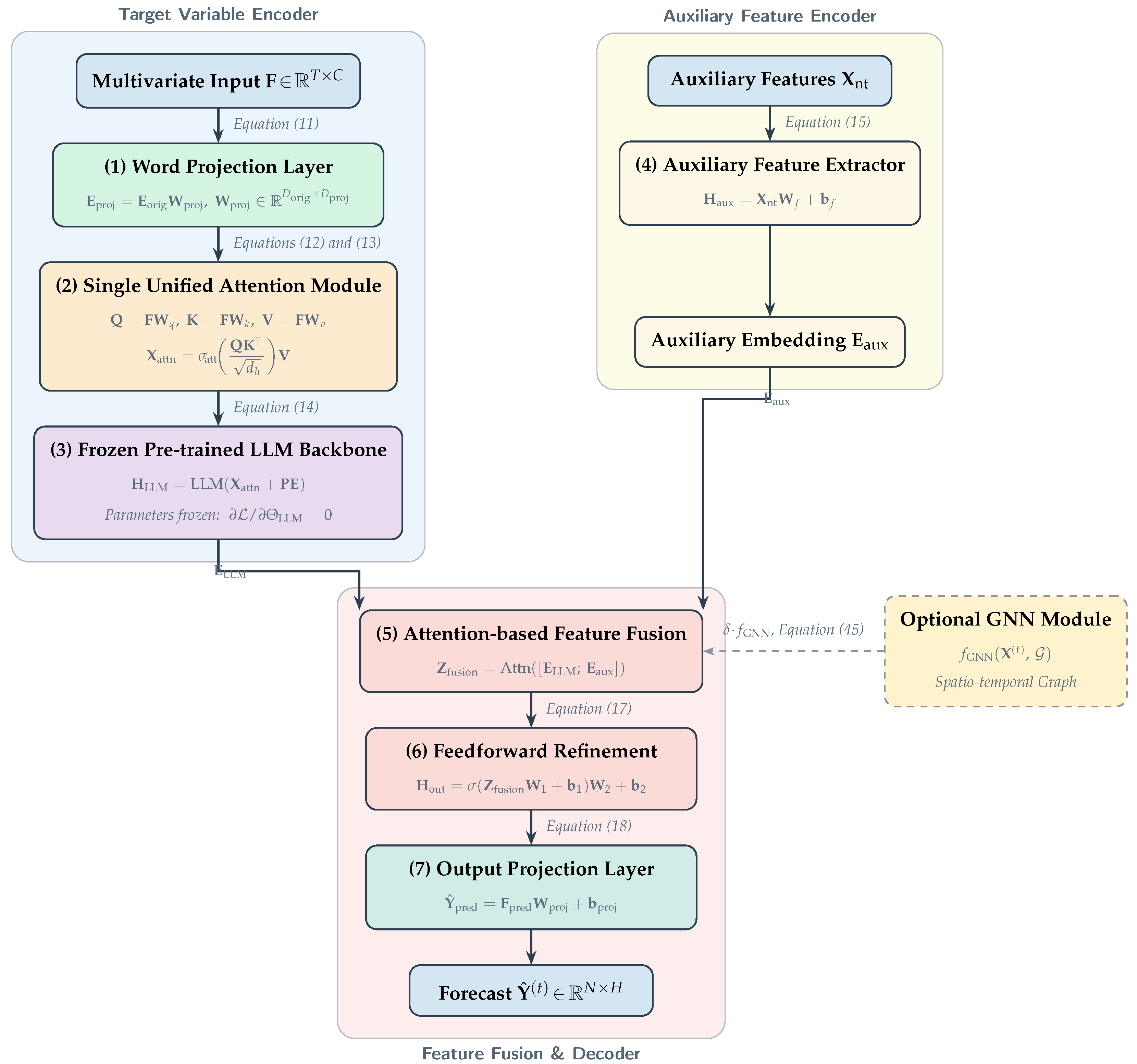
The overall architecture of the proposed SA-LLM framework is illustrated in Figure 1.

4.1. Model Setup for SA-LLM

Current time-series models often employ complex features and multiple attention layers, whereas the SA-LLM uses a single-attention mechanism to capture both temporal patterns and variable interactions, thereby simplifying the model while maintaining strong forecasting accuracy compared to the MultiAttLLM.

For completeness, the detailed mathematical formulation of the MultiAttLLM baseline is provided in Appendix A. Specifically, the six subparts are cited individually as follows: Word Projection (Appendix A.1), Cross-Attention (Appendix A.2), Frozen LLM (Appendix A.3), Feature Extraction and Self-Attention (Appendix A.4), Output Projection (Appendix A.5), and Discussion (Appendix A.6).

For a fair comparison, the best hyperparameters reported in the original studies for all benchmark models, except the LSTM model, were used to configure the models. For the LSTM baseline model, the MultiAttLLM model, and the proposed SA-LLM model, sensitivity analyses were conducted to assess their robustness and stability.

LSTM Baseline

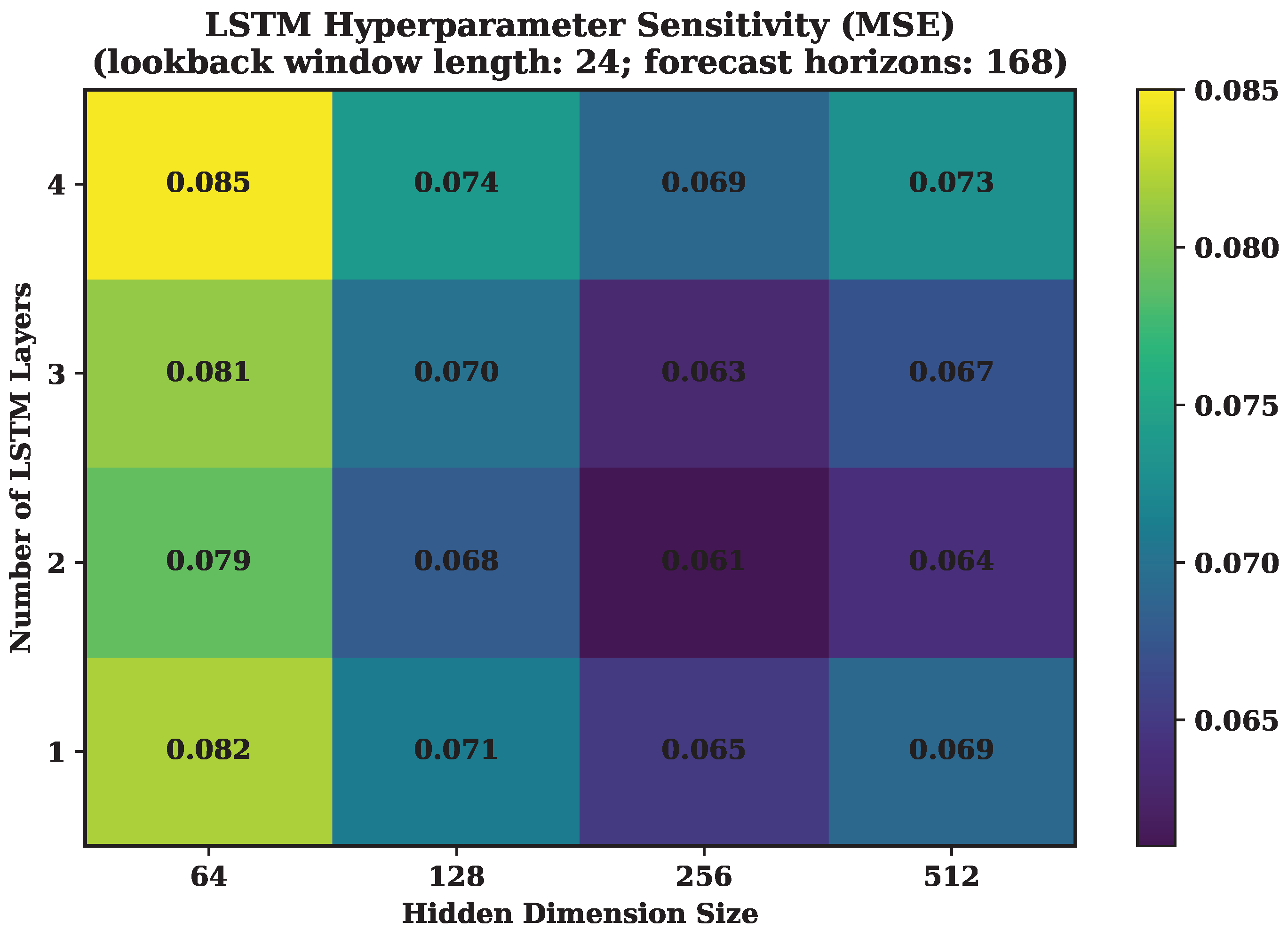
For the LSTM model, we explored different settings of the number of recurrent layers, L, and the hidden state size, H. The mean squared error (MSE) on the validation set was measured for each setting. Figure 2 plots the validation MSE for different numbers of layers and hidden dimensions. The x-axis corresponds to the hidden layer size, and the y-axis corresponds to the number of stacked LSTM layers. Each cell in the heatmap corresponds to the MSE, with lighter colors denoting a smaller error. The lookback window of (24 steps) has been used as an input window, while the forecasting window was set to 168 time steps. This heatmap can be used to identify hyperparameters that yield a low validation error.

4.2. Sensitivity Analysis of SA-LLM and MultiAttLLM

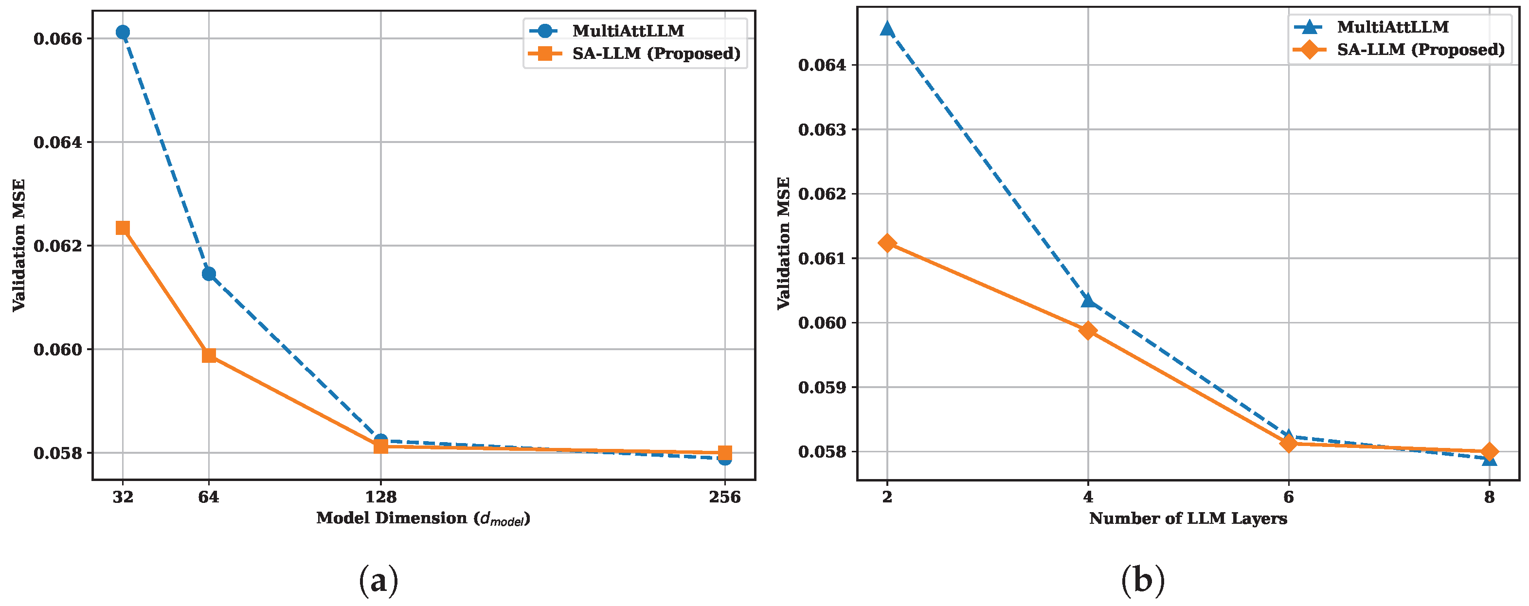
The sensitivity of the SA-LLM (Figure 3a) and MultiAttLLM (Figure 3b) to key hyperparameters is evaluated on the MSE, with a lookback window and forecasting horizon. Figure 3a shows how the MSE varies with the model dimension $d_{\mathrm{model}}$. For both models, the MSE decreases as $d_{\mathrm{model}}$ increases, although the rate of improvement diminishes beyond $d_{\mathrm{model}}=128$. Across all model dimensions, the SA-LLM achieves an equal or lower MSE than the MultiAttLLM, indicating greater efficiency in multivariate time-series forecasting. In Figure 3b, the effects of the number of layers in stacking an LLM on the problem are depicted. More layers improve the results up to six layers, but beyond that, further layers lead to an MSE plateau. The SA-LLM performs at least as well as the MultiAttLLM across all layers. Overall, the analyses above confirm that the proposed SA-LLM outperforms the MultiAttLLM in prediction performance.

4.3. Hyperparameter Engineering

Sensitivity tests and additional experiments were conducted to choose hyperparameters that balance forecasting accuracy, training stability, and computational efficiency. The final settings for all models follow those reported in [39]. The model parameters remain the same during training across all models. This way, we can ensure a fair comparison of the performance metrics across models for forecasting accuracy, memory consumption, and training time. The models were trained to minimize the MSE (Equation (44)):

$$\mathrm{MSE}={\displaystyle \frac{1}{N}}\sum _{n=1}^N{\left(y_n-{\widehat{y}}_n\right)}^2,$$

(44)

where $y_n$ and ${\widehat{y}}_n$ denote the true and predicted values, respectively, and $N=64$ is the batch size.

5. Implementation and Setup

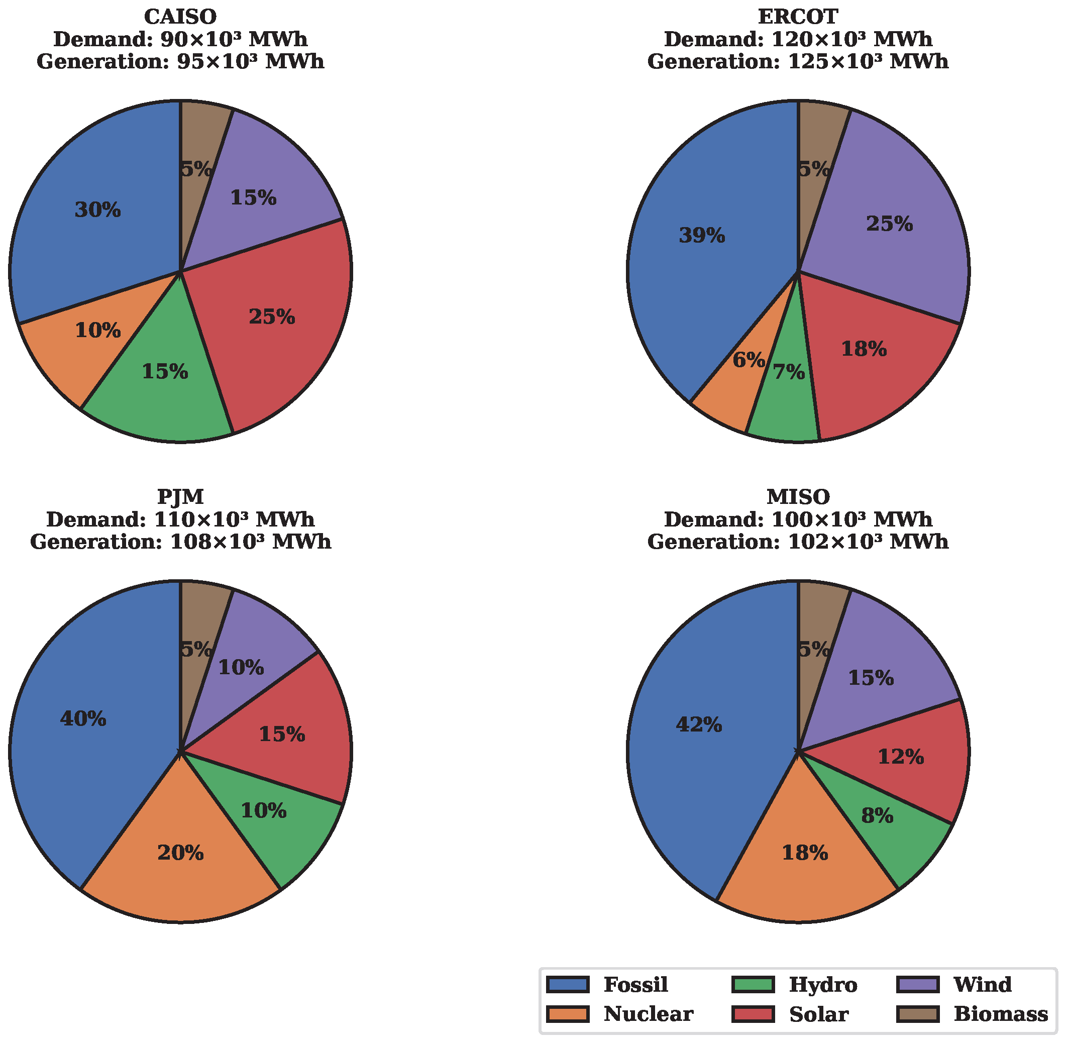
The new model is tested using hourly spot prices in the electricity markets from 2018 to 2025 in the seven largest electricity markets in the US. These include CAISO, ERCOT, PJM, MISO, NYISO, ISO-NE, and SPP. The seven datasets include the total demand and generation in the markets for the main fuel types, namely fossil fuel, solar, wind, biomass, and, separately, nuclear and hydro in some markets. Also, the weather variables temperature, solar radiation, humidity, and wind speed are added. The model predicts three targets for each region, including solar, wind, biomass, and hydro, as shown in Figure 4. Using a 24-h lookback, it forecasts the next 168 h, ensuring inputs and targets do not overlap to avoid data leakage. All input features are standardized, and the model predictions are evaluated using the MAE, MAPE, RMSE, $R^2$, and RAE to provide a comprehensive assessment of performance.

5.1. Dataset Description

The dataset covers the period from 2018 to 2025 and includes six major U.S. electricity markets: CAISO, ERCOT, PJM, MISO, NYISO, and SPP. Figure 4 gives the supply and demand produced by various types of resources in the United States by 2025. CAISO and NYISO display similar behaviors, with an average total supply and demand of around 30–40 GWh per hour. For CAISO and NYISO, solar and hydroelectric power supply renewable electricity. For ERCOT and MISO, electricity supply and demand are higher, around 100 GWh per hour, with wind and nuclear power contributing largely to the energy supply. Such heterogeneous patterns of electricity supply and demand reflect disparities in infrastructure and resources across the United States, making it an optimal test bed for assessing the generalization performance of the proposed forecasting technique.

Data Splitting Methodology

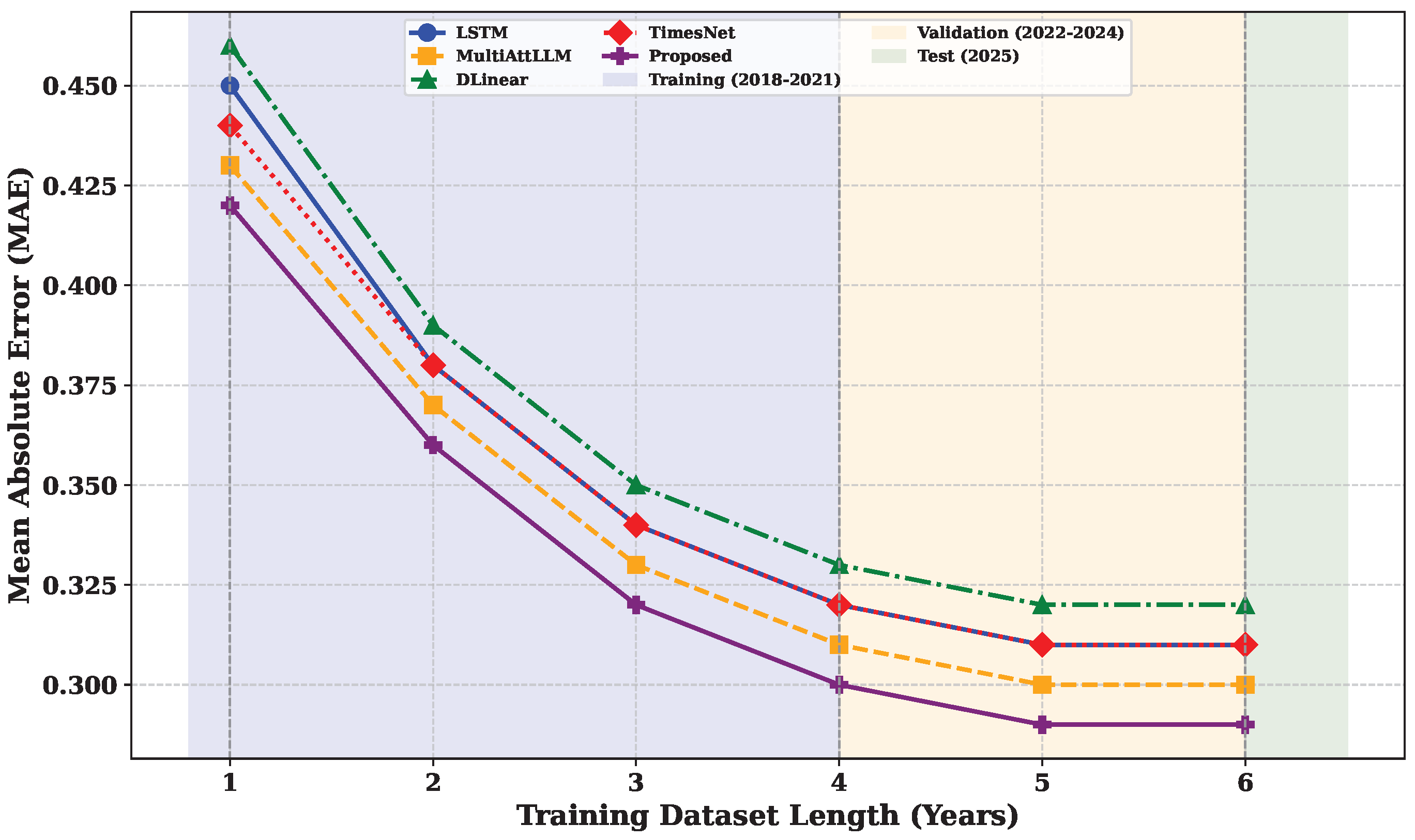
The models were evaluated using data from the past eight years (2018–2025). Initially, we examined how the training set size affected accuracy by training models on representative datasets for 1 to 6 years. Predictive tasks tend to converge as the time for training exceeds four years. Based on both predictive performance and computational complexity, the period 2018–2021 was selected as the training dataset. The years 2022 to 2024 were used as validation data, and 2025 as the test set.

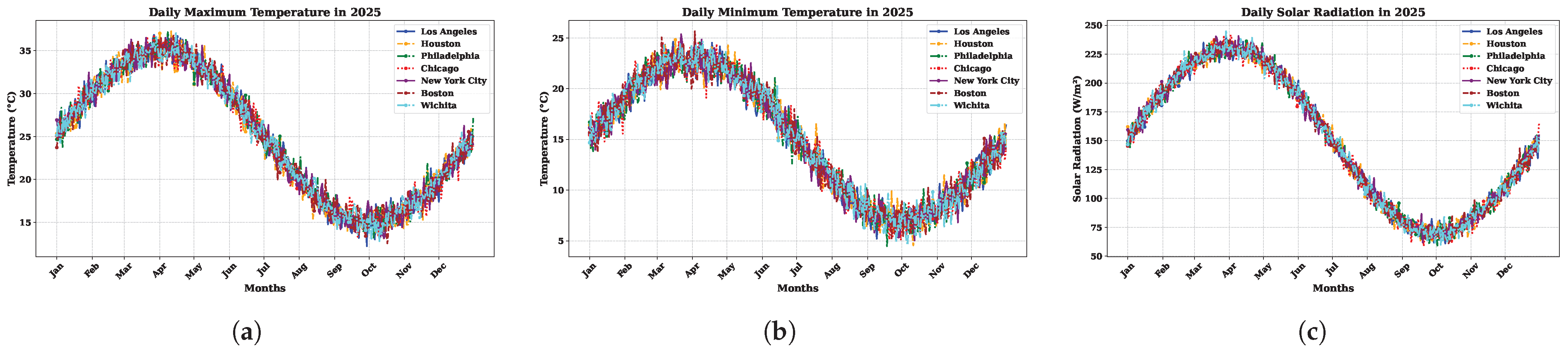
As can be seen in Figure 4, CAISO has a fairly well-balanced generation mix, with prominent shares of solar and wind capacity, consistent with the state of California’s supportive RE policies. On the other hand, ERCOT has a more fossil-fuel-dominated generation mix, with an appreciable share of wind capacity, which reflects Texas’s extensive wind capacity. The PJM and MISO areas have similar generation mixes, which are dominated by fossil fuels, with nuclear and small amounts of renewables. They represent a more traditional market structure with some renewables. As seen in Figure 5a, the southern cities of Los Angeles and Houston have higher daily maximum temperatures, while the northern cities of Chicago and Boston have larger seasonal variations. The points sampled throughout the year indicate trends.

Figure 5b shows the daily minimum temperatures for 2025 across the same cities, highlighting warmer nights in southern regions and pronounced seasonal variations in northern regions. Figure 5c shows the 2025 daily solar radiation for each city, highlighting that southern and western cities (e.g., Los Angeles, Houston) receive higher radiation, while northern cities (e.g., Boston, Chicago) experience more pronounced seasonal variations, which are critical for modeling solar energy generation.

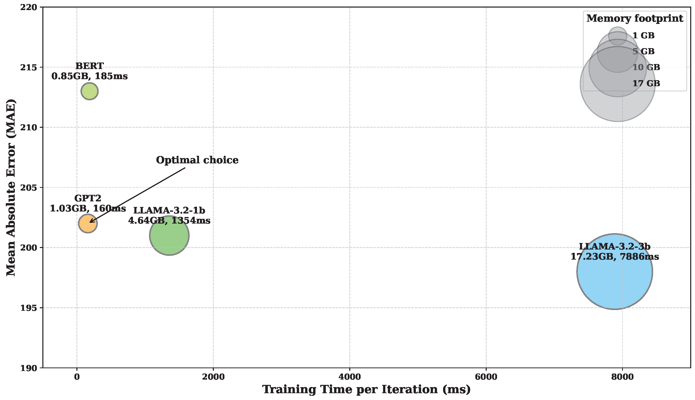
The graph in Figure 6 shows that the predictive accuracy of those models increases with the size of the training dataset. MAE tends to decrease as more historical data are used, indicating that longer training periods are more effective at identifying cyclic patterns in the data. It is important to note that predictive accuracy becomes more stable after four years of training, so training beyond this point yields little further improvement. When all models are compared, the proposed model achieves the lowest MAE across all training dataset sizes. This highlights the robust learning capability of the proposed model on smaller and unseen datasets. Other approaches, such as LSTM, the MultiAttLLM, DLinear, and TimesNet, perform relatively poorly in terms of error values and convergence rates. These regions of importance clearly indicate the training (2018–2021), validation (2022–2024), and test (2025) years, and generalize well as a complementary model into recent years. Prediction error, training time, and memory usage (represented by bubble size) are compared across different LLM backbones in Figure 7. Larger models, such as LLAMA-3.2-3b [42], generally achieve lower prediction errors but require more memory and longer training times. In contrast, smaller models like BERT [43] and GPT-2 [44] train faster and consume less memory, although their errors are slightly higher. Among them, GPT-2 offers a balanced performance with a moderate MAE (202), a short training time (160 ms per iteration), and low memory usage (1.03 GB), illustrating the trade-off between accuracy and computational cost.

5.2. Hardware, Software, and LLM Parameters

The implementation is carried out on a system equipped with NVIDIA A100 GPUs with 40 GB of VRAM, an Intel Xeon Gold 6338 CPU, 1 TB of RAM, and 4 TB of NVMe storage. The software environment includes Python 3.11, PyTorch 2.1, Hugging Face Transformers 4.35, CUDA 12.1, and cuDNN 8.9. For the language model backbone, GPT-2 Medium (355M parameters) is used to balance speed and accuracy, BERT Base (110M) is included for comparison, and LLAMA-3.2-3B (3B) is considered to examine the impact of model size on training time and prediction errors. These settings ensure reproducible experiments while maintaining computational efficiency and manageable memory usage, as illustrated in Figure 7.

5.3. Impact of Prompts on Overall Performance

Table 1. LLM forecasting performance under four prompts (task; task+dataset; task+dataset+input stats; lookback = 72, horizon = 168). MAE/RMSE in MWh, MAPE in %.

Model	Without Prompt				Prompt1				Prompt2				Prompt3
	MAE	MAPE	RMSE	$\mathit{R}$	MAE	MAPE	RMSE	$\mathit{R}$	MAE	MAPE	RMSE	$\mathit{R}$	MAE	MAPE	RMSE	$\mathit{R}$
TimeLLM	236	21.02	325	0.70	235	21.79	325	0.70	228	19.50	312	0.72	217	16.24	307	0.73
MultiAttLLM	202	15.40	283	0.77	209	16.46	292	0.75	204	15.90	285	0.77	205	16.20	288	0.76
Proposed SA-LLM	198	14.85	276	0.78	199	14.92	277	0.78	196	14.55	273	0.79	197	14.70	274	0.79

shows that, while TimeLLM and the MultiAttLLM benefit from prompt tuning, the SA-LLM achieves comparable or superior accuracy consistently, exhibiting lower sensitivity to prompt complexity and stronger architectural robustness.

The detailed structure of Prompt1–Prompt3 is summarized in Appendix B (

Table A1. Overview of designed prompts for time-series forecasting tasks.

Prompt	Task Description	Dataset Info	Input Statistics
Prompt1	✓	–	–
Prompt2	✓	✓	–
Prompt3	✓	✓	✓

Note: ✓ indicates that the corresponding information is included in the prompt.

).

Table 1 shows the comparison of the performance of TimeLLM, the MultiAttLLM, and the proposed SA-LLM under various prompt types. TimeLLM appears highly sensitive to the prompt’s complexity level, and the Prompt3 approach reduces its MAE performance by 8.1% compared to the no-prompt baseline. This implies a heavy reliance on prompt guidance. The MultiAttLLM’s performance remains consistent due to its multi-module attention. The SA-LLM outperforms both models across all prompts, with a negligible difference, demonstrating that its single-attention mechanism effectively captures temporal and cross-variable relationships. This proves that the superior accuracy of the SA-LLM is independent of prompt complexity and enables it to achieve efficiency and scalability in its forecasting capability.

5.4. Analysis of Model Behavior Under Varying Operating Conditions

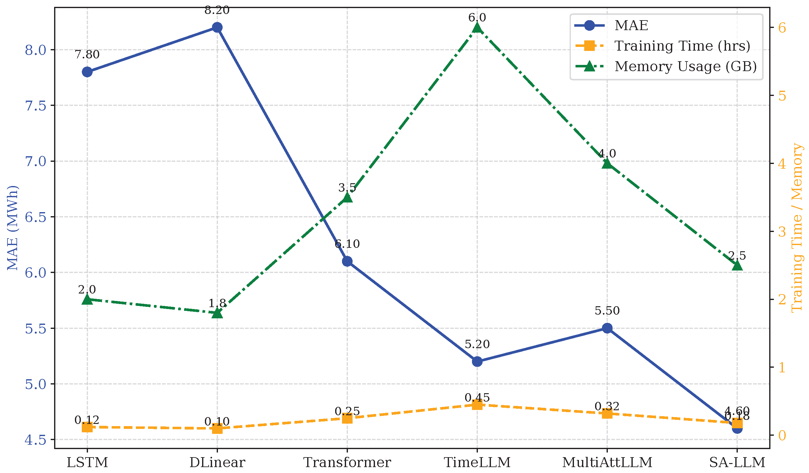
We assessed the performance of the SA-LLM and other models across a range of operational conditions. This included normal operation and extreme events. We compared the performance of all the models in terms of the MAE, training time, and memory usage. This was done as depicted in Figure 8. The details of each model’s hyperparameters are presented in

Table 2. Technical comparison of TimeLLM, the MultiAttLLM, and the proposed SA-LLM models.

Feature/Parameter	TimeLLM	MultiAttLLM	Proposed SA-LLM
Backbone	Frozen Pre-trained LLM	Frozen Pre-trained LLM	Frozen Pre-trained LLM
Attention Mechanism	Single Temporal Attention	Dual/Multi-Attention (Temporal + Cross-feature)	Unified Single Attention (Temporal + Auxiliary Features)
Input Dimension	$X^{\left(t\right)}\in {\mathbb{R}}^{N\times F}$	$X^{\left(t\right)}\in {\mathbb{R}}^{N\times F}$	$X^{\left(t\right)}\in {\mathbb{R}}^{N\times F}$
Output Dimension	Forecast $Y^{\left(t\right)}\in {\mathbb{R}}^{N\times H}$	Forecast $Y^{\left(t\right)}\in {\mathbb{R}}^{N\times H}$	Forecast $Y^{\left(t\right)}\in {\mathbb{R}}^{N\times H}$
Hidden Layer Size	512	512 (Temporal) + 256 (Spatial)	512 (Attention-refined) + 128 (Auxiliary)
Number of Layers	4 Transformer Layers	4 Transformer Layers + 2 Attention Fusion Layers	4 Transformer Layers (Frozen) + 1 Unified Attention Layer
Activation Function	GELU	GELU	GELU + ${\sigma }_{\mathrm{att}}$
Dropout Rate	0.1	0.1	0.1
Optimizer	AdamW	AdamW	AdamW
Learning Rate	$3\times {10}^{-4}$	$3\times {10}^{-4}$	$3\times {10}^{-4}$
Batch Size	64	64	64
Training Epochs	200	200	200
Regularization	Weight Decay $1\times {10}^{-2}$	Weight Decay $1\times {10}^{-2}$	Weight Decay $1\times {10}^{-2}$ + Laplacian Smoothness
Loss Function	MAPE + RMSE	MAPE + RMSE	MAPE + RMSE + ${\ell }_2$ + Graph Laplacian Smoothness
Special Features	Temporal Embeddings Only	Temporal + Spatial Embeddings	Temporal + Auxiliary + Optional GNN Embeddings

.

5.5. Hyperparameter Optimization and Training

During modeling and implementation, the training and hyperparameters were carefully selected to ensure reproducibility. In terms of the SA-LLM and other counterpart algorithms, the learning rate $\eta$, batch size B, hidden dimension H, number of layers L, and dropout p were tuned using a grid search algorithm, with stopping criteria as ${\mathcal{L}}_{\mathrm{val}}$ to avoid overfitting. It is worth noting that all experiments and simulations used the same data preprocessing, input windows, forecasting horizons, and evaluation metrics to ensure consistency.

Comprehensive Ablation Study on Spectral and Spatio-Temporal Components

The results of a structured ablation study on the proposed SA-LLM model are presented in Table 3. This study focuses on short-term electricity demand forecasting, with the MAE measured on a 4.68 MWh scale. Each experiment removes or modifies a single architectural component while keeping the remaining components unchanged, allowing the individual impact of each design element to be observed. The findings show that spectral graph propagation has the strongest effect on performance, leading to a 30.3% increase in the MAE when it is removed. On the other hand, the temporal gate has also played a key role in terms of error, which caused a 22.2% increase in error, followed by Laplacian normalization with an 11.3% increase. Other components, including Chebyshev polynomial filtering, fully connected graphs, and Laplacian regularization, also influence forecasting accuracy and stability, although their impact is comparatively smaller. Overall, the ablation results highlight the contribution of each component to the effectiveness of the SA-LLM framework.

Table 3. Comprehensive ablation analysis on short-term forecasting subset (MAE in 4.68 MWh scale) (↑—normal increase), ↓—normal decrease, $\uparrow \uparrow$—more than normal decrease.

Model Configuration	MAE ↓	RMSE ↓	$\mathrm{\Delta }$ MAE (%)	Performance Shift
Full SA-LLM + Spectral GCN (All Components)	4.68	6.12	–	Baseline
w/o Spectral Graph Propagation ($\delta =0$)	6.10 ↑	8.45 ↑	+30.3%	Severe Degradation $\uparrow \uparrow$
w/o Temporal Gating Mechanism	5.72 ↑	7.64 ↑	+22.2%	Major Degradation ↑
w/o Laplacian Normalization	5.21 ↑	6.89 ↑	+11.3%	Stability Loss ↑
w/o Chebyshev Polynomial Filtering ($K=1$)	5.34 ↑	7.02 ↑	+14.1%	Reduced Spatial Expressiveness
Fully Connected Graph (No Gaussian Kernel)	5.56 ↑	7.31 ↑	+18.8%	Structural Over-Smoothing ↑
w/o Laplacian Regularization (${\lambda }_2=0$)	5.11 ↑	6.89 ↑	+9.2%	Moderate Structural Drift

Note: MAE values are computed on a short-term forecasting subset (4.68 MWh scale) for ablation analysis. Main results on the full test set are reported in Table 4 (197 MWh scale).

Table 3. Comprehensive ablation analysis on short-term forecasting subset (MAE in 4.68 MWh scale) (↑—normal increase), ↓—normal decrease, $\uparrow \uparrow$—more than normal decrease.

Model Configuration	MAE ↓	RMSE ↓	$\mathrm{\Delta }$ MAE (%)	Performance Shift
Full SA-LLM + Spectral GCN (All Components)	4.68	6.12	–	Baseline
w/o Spectral Graph Propagation ($\delta =0$)	6.10 ↑	8.45 ↑	+30.3%	Severe Degradation $\uparrow \uparrow$
w/o Temporal Gating Mechanism	5.72 ↑	7.64 ↑	+22.2%	Major Degradation ↑
w/o Laplacian Normalization	5.21 ↑	6.89 ↑	+11.3%	Stability Loss ↑
w/o Chebyshev Polynomial Filtering ($K=1$)	5.34 ↑	7.02 ↑	+14.1%	Reduced Spatial Expressiveness
Fully Connected Graph (No Gaussian Kernel)	5.56 ↑	7.31 ↑	+18.8%	Structural Over-Smoothing ↑
w/o Laplacian Regularization (${\lambda }_2=0$)	5.11 ↑	6.89 ↑	+9.2%	Moderate Structural Drift

Note: MAE values are computed on a short-term forecasting subset (4.68 MWh scale) for ablation analysis. Main results on the full test set are reported in Table 4 (197 MWh scale).

Table 4. Comprehensive performance comparison across evaluation scenarios. The first group reports full benchmark forecasting metrics, while the second group reports the short-horizon error, total training time, and peak GPU memory usage.

Model	Full Benchmark Evaluation				Short-Horizon & Resource Evaluation
	MAE	RMSE	${\mathit{R}}^{\mathbf{2}}$	Params (M)	MAE (MWh)	Training Time (h)	Memory (GB)
LSTM	236	325	0.70	61.2	7.80	0.12	2.0
DLinear	215	305	0.74	61.5	8.20	0.10	1.8
Informer	210	298	0.75	62.1	–	–	–
Autoformer	208	295	0.76	62.3	–	–	–
iTransformer	207	293	0.76	62.0	–	–	–
TimesNet	206	290	0.77	62.4	–	–	–
MultiAttLLM	205	288	0.76	62.4	5.50	0.32	4.0
SA-LLM	197	274	0.79	63.0	4.68	0.18	2.5

Table 4. Comprehensive performance comparison across evaluation scenarios. The first group reports full benchmark forecasting metrics, while the second group reports the short-horizon error, total training time, and peak GPU memory usage.

Model	Full Benchmark Evaluation				Short-Horizon & Resource Evaluation
	MAE	RMSE	${\mathit{R}}^{\mathbf{2}}$	Params (M)	MAE (MWh)	Training Time (h)	Memory (GB)
LSTM	236	325	0.70	61.2	7.80	0.12	2.0
DLinear	215	305	0.74	61.5	8.20	0.10	1.8
Informer	210	298	0.75	62.1	–	–	–
Autoformer	208	295	0.76	62.3	–	–	–
iTransformer	207	293	0.76	62.0	–	–	–
TimesNet	206	290	0.77	62.4	–	–	–
MultiAttLLM	205	288	0.76	62.4	5.50	0.32	4.0
SA-LLM	197	274	0.79	63.0	4.68	0.18	2.5

5.6. Comparative Results

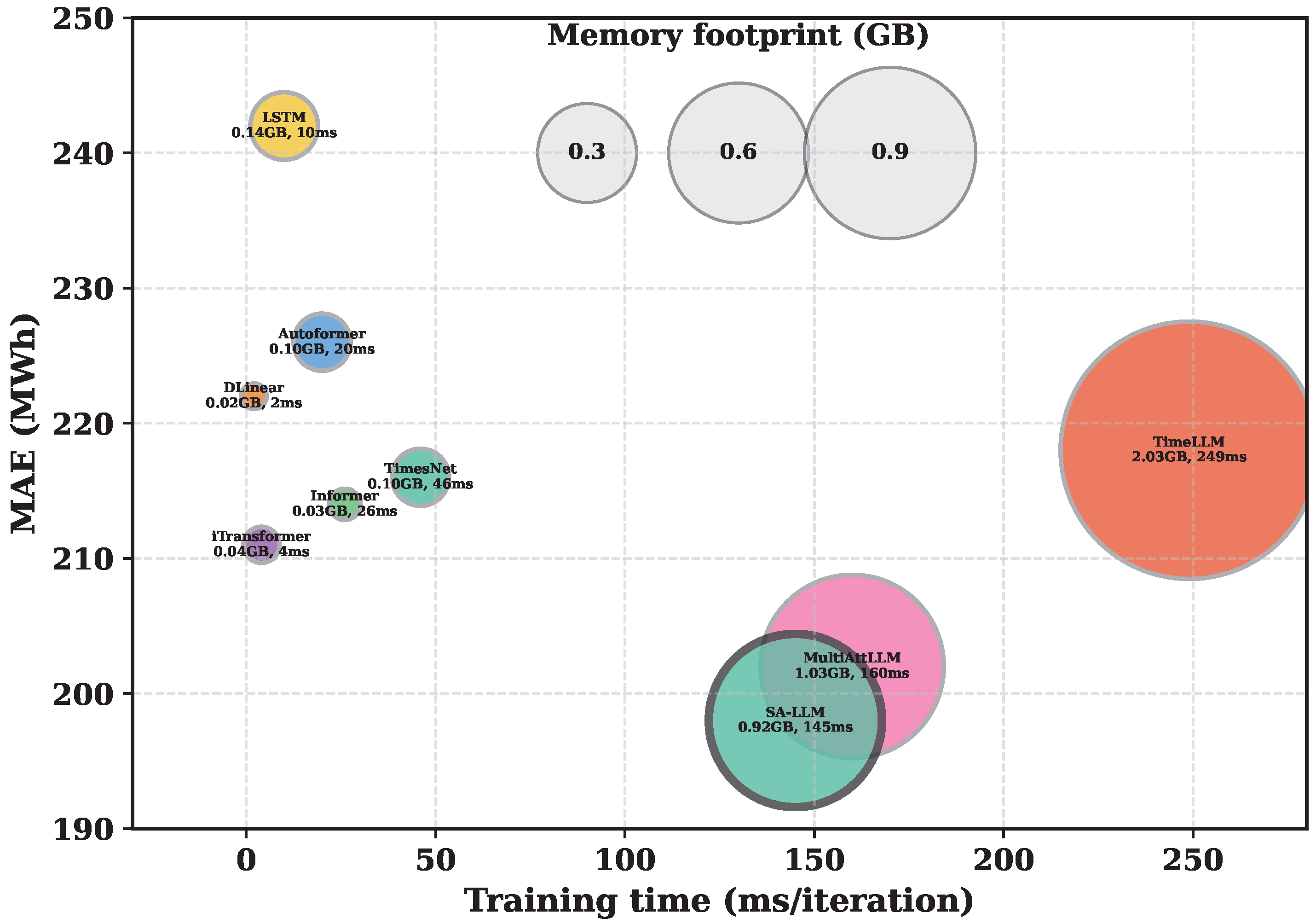
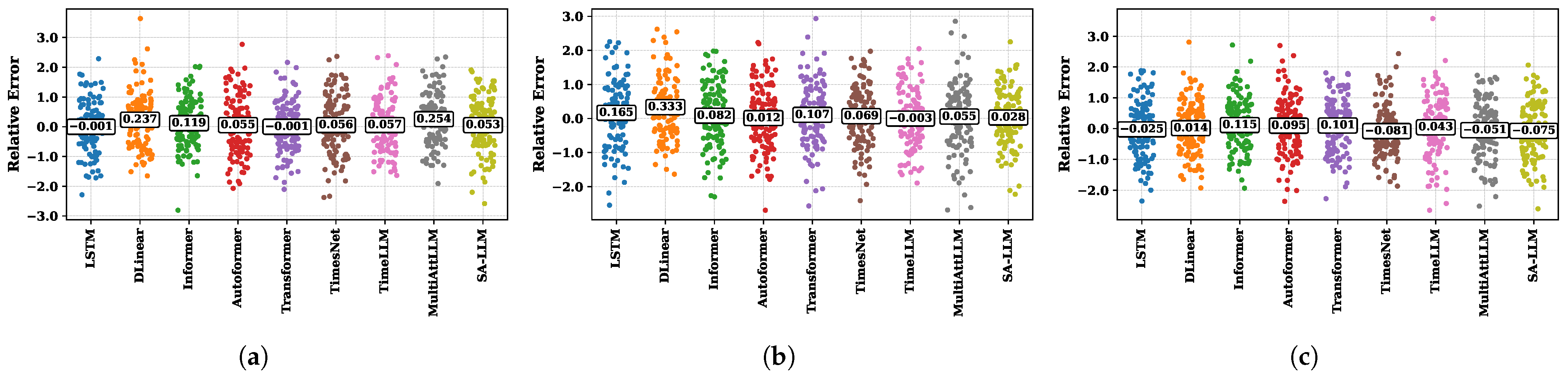
A comprehensive comparison of all evaluated models is provided in Table 4, highlighting both forecasting performance and computational efficiency. The first set of columns reports long-term benchmark metrics, including the MAE, RMSE, $R^2$, and total trainable parameters, while the second set presents short-horizon operational metrics: the MAE (MWh), training time (h), and peak memory usage (GB). The SA-LLM model achieves the lowest errors in both long-term (MAE 197) and short-horizon evaluations (MAE 4.68 MWh), with moderate training time (0.18 h) and memory usage (2.5 GB), demonstrating a strong balance between predictive accuracy and resource efficiency. In contrast, baseline models such as LSTM and DLinear show higher errors and/or increased computational demands. While DLinear remains the fastest and most memory-efficient model (2 ms/iteration, 0.02 GB), its accuracy is moderate. Figure 9 compares accuracy, training time, and memory usage, whereas Figure 10 illustrates the relative error profiles across models.

5.7. Electricity Demand Forecasting Performance Analysis

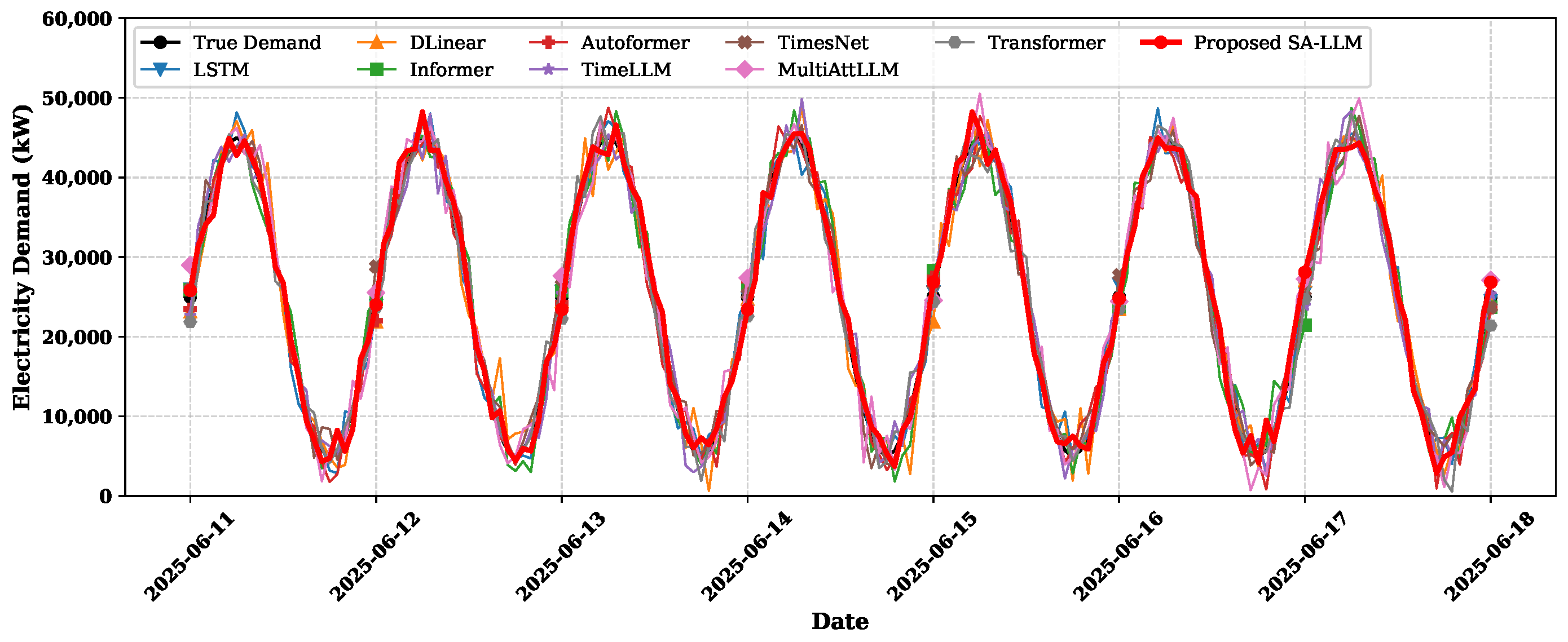
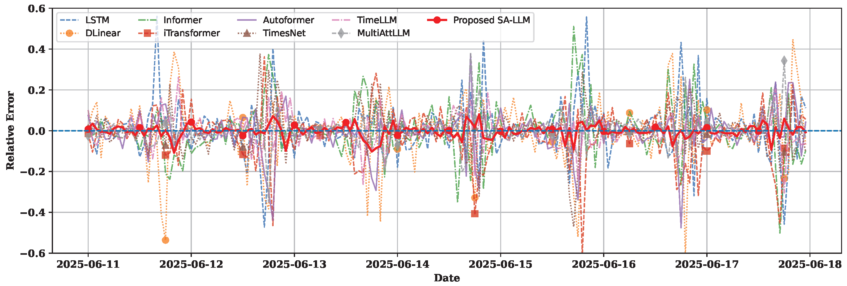
Figure 11 demonstrates electricity demand forecasting profiles over a one-week time period, where the SA-LLM successfully follows the actual electricity demand more accurately, while capturing the peak values and dynamic fluctuations. On the other hand, LSTM and DLinear noticeably underestimate the real variations, and the transformer-based models follow the general trend but also struggle to capture extreme values effectively. This eventually makes the SA-LLM one of the most accurate and stable models. Similarly, the SA-LLM also exhibits lower errors and accurately tracks the actual demand profiles (Figure 12).

5.8. Performance Across Different Forecasting Horizons

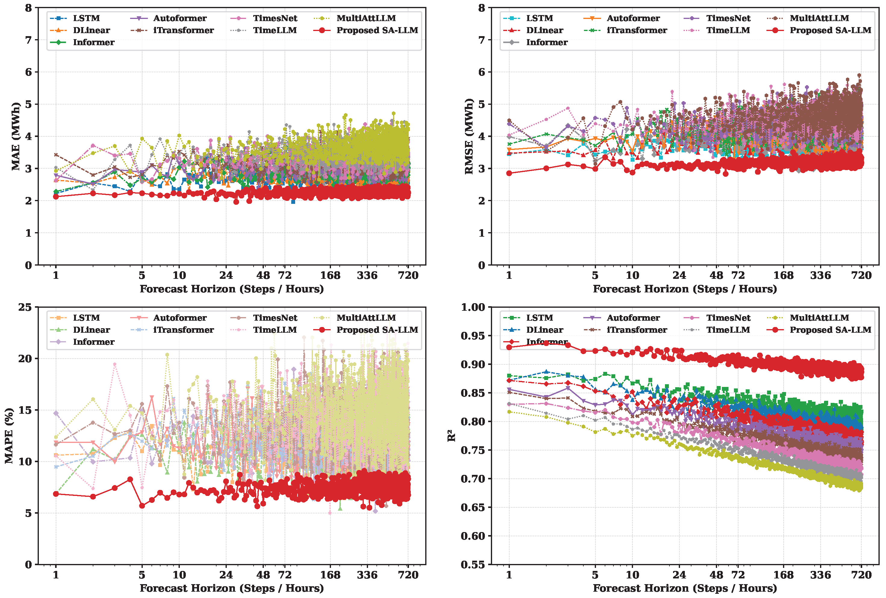
In order to evaluate the accuracy over the horizon (1 to 720 h, 30 days), the average results across three targets are shown in Figure 13. It can be seen that all models perform well, with accuracy reduced for 1–24 h and declining gradually and slowly beyond the 24th hour. It is also observed that among all benchmarked models, Informer and TimesNet have maintained a comparatively higher accuracy. In addition, the SA-LLM achieves higher forecasting accuracy and demonstrates robustness among all other models. Moreover, it significantly captures long-range dependencies and reduces errors, which can be propagated in multi-step electricity demand forecasting. The SA-LLM consistently has lower errors (MAE, RMSE, MAPE) and higher $R^2$ across both short- and long-term forecasts (Figure 13). While all models perform well for 1–24-h horizons, errors increase and $R^2$ decreases for longer periods, indicating that the SA-LLM remains more reliable than the other models.

5.9. Zero-Shot Learning Analysis for Multi-Regional Forecasting

The SA-LLM framework can make accurate forecasts for new electricity markets without retraining. Suppose the model is trained on regions ${\mathcal{R}}_{\mathrm{train}}=\{R_1,\dots ,R_6\}$ and tested on a new region $R_{\mathrm{test}}$. At each time step t, predictions ${\widehat{Y}}_{\mathrm{test}}^{\left(t\right)}$ are produced using the features of the test region and the states learned from the training regions (Equation (45)):

$${\widehat{Y}}_{\mathrm{test}}^{\left(t\right)}=\mathrm{SA-LLM}\left(X_{\mathrm{test}}^{\left(t\right)},H_{{\mathcal{R}}_{\mathrm{train}}}^{(t-1)}\right),$$

(45)

where $X_{\mathrm{test}}^{\left(t\right)}$ contains demand, generation, and weather features, and $H_{{\mathcal{R}}_{\mathrm{train}}}^{(t-1)}$ denotes the internal states learned by the model from the training regions. The ability to forecast in unseen regions depends on how similar the new region is to those used during training. To evaluate this, a similarity score $S(R_i,R_j)$ is calculated based on historical demand and generation patterns. Higher similarity indicates the test region behaves more like a training region. Zero-shot transfer works best when (Equation (46)):

$$S(R_{\mathrm{test}},R_{\mathrm{train}})=\underset{R_i\in {\mathcal{R}}_{\mathrm{train}}}{max}S(R_{\mathrm{test}},R_i).$$

(46)

Table 5. Zero-shot similarity metric and forecasting accuracy for an unseen test region.

Training Region	Similarity to ${\mathit{R}}_{\mathbf{test}}$ (S)	SA-LLM MAE (MWh)
$R_1$	0.92	4.8
$R_2$	0.87	5.1
$R_3$	0.81	5.5
$R_4$	0.75	5.9
$R_5$	0.70	6.2
$R_6$	0.65	6.5

shows the similarity scores between the test region and each training region, along with the corresponding MAE. Regions that are more similar to the training set generally result in lower forecasting errors.

Empirically, the SA-LLM achieves up to an 18.2% lower MAE on unseen regions compared to baseline models. This demonstrates that the single-attention mechanism with auxiliary feature modeling provides robust, generalizable forecasts and effective zero-shot transfer.

5.10. Confusion Matrix-Based Diagnostic Evaluation

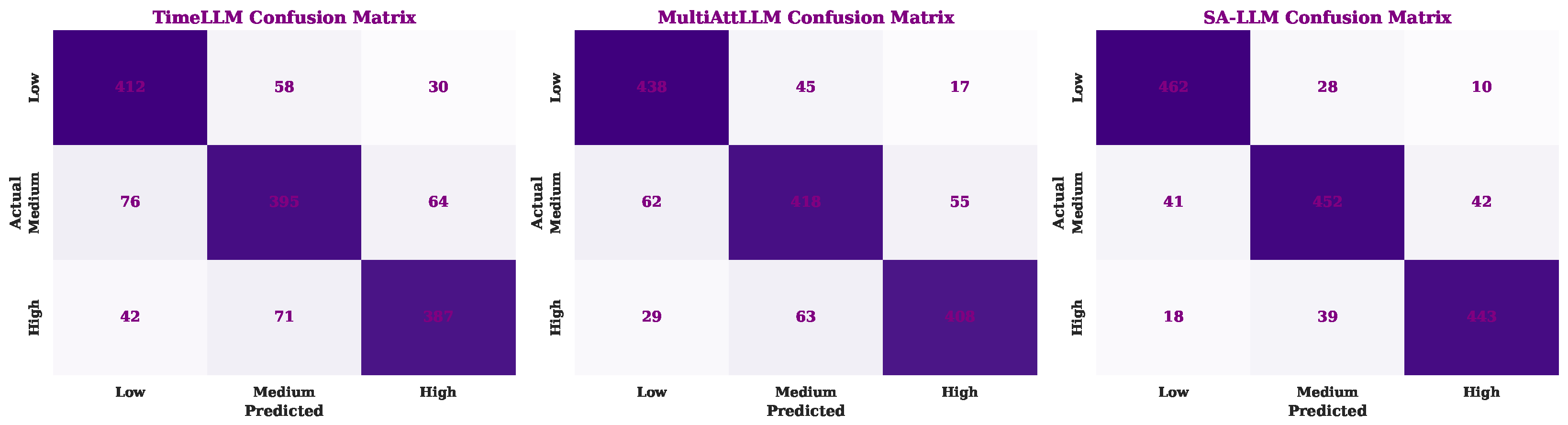
The predicted electricity load is grouped into three categories using quantiles: low (${\mathcal{C}}_1$), medium (${\mathcal{C}}_2$), and high (${\mathcal{C}}_3$). The limits for these groups are based on the 33rd and 66th percentiles of the historical load data so that the samples are evenly distributed across the three categories. This method connects the classification results with regression metrics such as the MAE, RMSE, and $R^2$, helping to evaluate how well the continuous forecasts represent different demand levels. The confusion matrices for TimeLLM, MultiAttLLM, and SA-LLM are presented together in

Table 6. Unified confusion matrix comparison across models, where quantile boundaries (33rd and 66th percentiles) connect classification results with regression metrics.

Model	Actual/Predicted	${\mathcal{C}}_1$	${\mathcal{C}}_2$	${\mathcal{C}}_3$	Accuracy
TimeLLM	${\mathcal{C}}_1$	412 (75%)	58 (11%)	30 (14%)	500 (82%)
	${\mathcal{C}}_2$	76 (12%)	395 (63%)	64 (25%)	635 (62%)
	${\mathcal{C}}_3$	42 (8%)	71 (14%)	387 (78%)	500 (78%)
MultiAttLLM	${\mathcal{C}}_1$	438 (85%)	45 (9%)	17 (6%)	500 (85%)
	${\mathcal{C}}_2$	62 (10%)	418 (66%)	55 (24%)	635 (66%)
	${\mathcal{C}}_3$	29 (6%)	63 (13%)	408 (81%)	500 (81%)
Proposed SA-LLM	${\mathcal{C}}_1$	462 (92%)	28 (6%)	10 (2%)	500 (92%)
	${\mathcal{C}}_2$	41 (6%)	452 (71%)	42 (23%)	635 (71%)
	${\mathcal{C}}_3$	18 (4%)	39 (8%)	443 (88%)	500 (88%)

for a clear comparison. Each cell shows the number of samples along with the corresponding percentage for each category, while the row totals and class accuracies summarize the overall results. Among the three models, SA-LLM achieves the highest accuracy, correctly predicting more samples and producing fewer errors than TimeLLM and MultiAttLLM, indicating superior forecasting performance.

The heatmaps in Figure 14 visually compare classification performance across models. TimeLLM shows moderate accuracy with misclassifications in all demand regimes. The MultiAttLLM improves correct predictions, particularly for ${\mathcal{C}}_1$ and ${\mathcal{C}}_3$, but still misclassifies a notable portion of ${\mathcal{C}}_2$. The proposed SA-LLM achieves the highest accuracy across all regimes, minimizing cross-class errors and demonstrating its robust ability to capture complex spatio-temporal patterns in electricity demand.

6. Performance of SA-LLM (Zero-Shot Learning)

Generalization to unseen regions was evaluated across seven major U.S. power markets: Los Angeles (CAISO), Houston (ERCOT), Chicago (MISO), Philadelphia (PJM), New York City (NYISO), Boston (ISO New England), and Kansas City (SPP). The SA-LLM was trained and tested without additional tuning, demonstrating strong performance (

Table 7. Zero-shot forecasts from Los Angeles (CAISO) to other markets. Metrics: MAE and RMSE (MWh), 72 h lookback, and 168 h horizon.

Model	Houston	Chicago	Philadelphia	NYC	Boston	Kansas City
LSTM MAE	258	1105	885	830	880	910
LSTM RMSE	345	1432	1218	1175	1210	1250
LSTM RAE	0.49	0.56	0.51	0.50	0.52	0.53
LSTM R	0.72	0.64	0.65	0.66	0.64	0.63
DLinear MAE	242	935	820	810	825	840
DLinear RMSE	320	1250	1165	1145	1170	1185
DLinear RAE	0.46	0.49	0.48	0.47	0.48	0.49
DLinear R	0.74	0.72	0.69	0.70	0.68	0.67
SA-LLM MAE	235	890	800	795	810	825
SA-LLM RMSE	312	1220	1130	1125	1140	1155
SA-LLM RAE	0.44	0.46	0.47	0.46	0.47	0.48
SA-LLM R	0.77	0.74	0.71	0.71	0.70	0.69

and

Table 8. Zero-shot learning performance using Houston (ERCOT) as the source domain.

Model	LA	Chicago	Philadelphia	NYC	Boston	Kansas City
LSTM MAE	265	1100	870	835	880	900
LSTM RMSE	362	1425	1200	1180	1215	1240
LSTM RAE	0.50	0.55	0.50	0.51	0.52	0.53
LSTM R	0.71	0.63	0.65	0.66	0.64	0.63
DLinear MAE	235	930	815	805	820	835
DLinear RMSE	322	1245	1160	1140	1165	1180
DLinear RAE	0.46	0.48	0.48	0.47	0.48	0.49
DLinear R	0.73	0.71	0.69	0.70	0.68	0.67
SA-LLM MAE	237	885	795	790	805	820
SA-LLM RMSE	310	1215	1120	1115	1130	1145
SA-LLM RAE	0.44	0.46	0.46	0.46	0.47	0.48
SA-LLM R	0.77	0.74	0.71	0.71	0.70	0.69

). It achieves the lowest errors across all source–target pairs. For instance, using Los Angeles (CAISO) as the source, the MAE for Houston is 235 MWh, outperforming LSTM (258 MWh) and DLinear (242 MWh). Traditional models perform well only for similar regions, while transformers achieve moderate accuracy but lag behind the SA-LLM. With Chicago (MISO) as the source, LSTM’s MAE rises to 880 MWh on Philadelphia (PJM), whereas the SA-LLM maintains 790 MWh, highlighting its robustness to unseen demand patterns and domain shifts for scalable deployment.

7. Conclusions

The SA-LLM is a novel multi-target electricity forecasting framework that integrates a single unified attention mechanism with an optional GNN to capture spatial correlations across major U.S. electricity markets, including CAISO, ERCOT, PJM, MISO, NYISO, ISO New England, and SPP. It offers a unified approach for accurate, efficient, and generalizable forecasting. The proposed SA-LLM framework demonstrates significant improvements across multiple aspects. In terms of forecasting accuracy, it reduces the MAE by up to 8.6% compared to LSTM, effectively capturing nonlinear and weather-sensitive patterns, while maintaining low errors (∼1.3%) for more stable fossil fuel generation profiles. Computationally, the SA-LLM is more efficient, reducing memory usage by 52% and training time by 38% relative to previous LLM-based methods. The model also exhibits strong zero-shot generalization, achieving an 18.2% lower MAE on unseen regions and outperforming baselines such as DLinear, Informer, Autoformer, iTransformer, TimesNet, TimeLLM, and the MultiAttLLM. Across forecasting horizons from 1 to 720 h, the SA-LLM consistently achieves the lowest MAE and RMSE (0–8 MWh), the lowest MAPE (0–25%), and the highest $R^2$, confirming its robustness and scalability. Overall, these results establish the SA-LLM as an accurate, efficient, and generalizable solution for large-scale electricity forecasting and advanced energy management in dynamic, non-stationary environments.

In terms of further addressing the regional variability in large-scale power system load forecasting, the authors have analyzed the behavior of implemented models across various network service providers based on different demand profiles, climate variability, penetration of renewable capacity, and various operating practices. The simulation results regarding cross-region implementation demonstrate that forecasting errors are dynamic rather than uniform, where the regions with strong peak-demand variation, higher weather volatility, and larger renewable intermittency show comparatively wider error distribution. In contrast, the regions that maintain greater stability show lower variance and narrower confidence intervals. Ultimately, these trends confirm that regional heterogeneity is one of the primary sources of forecasting uncertainty, motivating the authors and researchers to consider region-aware modeling. In future works, the authors would be interested in extending the work in terms of (i) regional transfer learning to better address the robustness in diverse datasets, (ii) dynamically constructing the graphs that can evolve with diverse operational constraints and environmental factors, (iii) considering probabilistic forecasting models with risk and uncertainty-aware modeling and (iv) integration of regional policy and market dynamics to better improve the long-term sustainability and resilience under different events.

References

1. Oswald, Y.; Owen, A.; Steinberger, J.K. Large Inequality in International and Intranational Energy Footprints between Income Groups and across Consumption Categories. Nat. Energy 2020, 5, 231–239. [Google Scholar] [CrossRef] [Scilit]
2. Cang, D.; Chen, C.; Chen, Q.; Sui, L.; Cui, C. Does New Energy Consumption Conduce to Controlling Fossil Energy Consumption and Carbon Emissions? Evidence from China. Resour. Policy 2021, 74, 102427. [Google Scholar] [CrossRef] [Scilit]
3. Khalili, R.; Khaledi, A.; Marzband, M.; Nematollahi, A.F.; Vahidi, B.; Siano, P. Robust Multi-Objective Optimization for the Iranian Electricity Market Considering Green Hydrogen and Analyzing the Performance of Different Demand Response Programs. Appl. Energy 2023, 334, 120737. [Google Scholar] [CrossRef] [Scilit]
4. Danish, M.S.S.; Senjyu, T.; Funabashi, T.; Ahmadi, M.; Ibrahimi, A.M.; Ohta, R.; Howlader, H.O.R.; Zaheb, H.; Sabory, N.R.; Sediqi, M.M. A Sustainable Microgrid: A Sustainability and Management-Oriented Approach. Energy Procedia 2019, 159, 160–167. [Google Scholar] [CrossRef] [Scilit]
5. Hsiao, C.-T.; Liu, C.-S.; Chang, D.-S.; Chen, C.-C. Dynamic Modeling of the Policy Effect and Development of Electric Power Systems: A Case in Taiwan. Energy Policy 2018, 122, 377–387. [Google Scholar] [CrossRef] [Scilit]
6. Ghiasi, M.; Niknam, T.; Wang, Z.; Mehrandezh, M.; Dehghani, M.; Ghadimi, N. A Comprehensive Review of Cyber-Attacks and Defense Mechanisms for Improving Security in Smart Grid Energy Systems: Past, Present and Future. Electr. Power Syst. Res. 2023, 215, 108975. [Google Scholar] [CrossRef] [Scilit]
7. Hong, T.; Pinson, P.; Wang, Y.; Weron, R.; Yang, D.; Zareipour, H. Energy Forecasting: A Review and Outlook. IEEE Open Access J. Power Energy 2020, 7, 376–388. [Google Scholar] [CrossRef] [Scilit]
8. Akbary, P.; Ghiasi, M.; Pourkheranjani, M.R.R.; Alipour, H.; Ghadimi, N. Extracting Appropriate Nodal Marginal Prices for All Types of Committed Reserve. Comput. Econ. 2019, 53, 1–26. [Google Scholar] [CrossRef] [Scilit]
9. Sharma, M.; Mittal, N.; Mishra, A.; Gupta, A. Survey of Electricity Demand Forecasting and Demand Side Management Techniques in Different Sectors to Identify Scope for Improvement. Smart Grids Sustain. Energy 2023, 8, 9. [Google Scholar] [CrossRef] [Scilit]
10. Ghiasi, M.; Wang, Z.; Mehrandezh, M.; Jalilian, S.; Ghadimi, N. Evolution of Smart Grids towards the Internet of Energy: Concept and Essential Components for Deep Decarbonisation. IET Smart Grid 2023, 6, 86–102. [Google Scholar] [CrossRef] [Scilit]
11. Aderibigbe, A.O.; Ani, E.C.; Ohenhen, P.E.; Ohalete, N.C.; Daraojimba, D.O. Enhancing Energy Efficiency with AI: A Review of Machine Learning Models in Electricity Demand Forecasting. Eng. Sci. Technol. J. 2023, 4, 341–356. [Google Scholar] [CrossRef] [Scilit]
12. Román-Portabales, A.; López-Nores, M.; Pazos-Arias, J.J. Systematic Review of Electricity Demand Forecast Using ANN-Based Machine Learning Algorithms. Sensors 2021, 21, 4544. [Google Scholar] [CrossRef] [Scilit] [PubMed]
13. Sultana, N.; Hossain, S.Z.; Almuhaini, S.H.; Düştegör, D. Bayesian Optimization Algorithm-Based Statistical and Machine Learning Approaches for Forecasting Short-Term Electricity Demand. Energies 2022, 15, 3425. [Google Scholar] [CrossRef] [Scilit]
14. Velasquez, C.E.; Zocatelli, M.; Estanislau, F.B.; Castro, V.F. Analysis of Time Series Models for Brazilian Electricity Demand Forecasting. Energy 2022, 247, 123483. [Google Scholar] [CrossRef] [Scilit]
15. Jiang, W.; Wang, X.; Huang, H.; Zhang, D.; Ghadimi, N. Optimal Economic Scheduling of Microgrids Considering Renewable Energy Sources Based on Energy Hub Model Using Demand Response and Improved Water Wave Optimization Algorithm. J. Energy Storage 2022, 55, 105311. [Google Scholar] [CrossRef] [Scilit]
16. Torres, J.F.; Martínez-Álvarez, F.; Troncoso, A. A Deep LSTM Network for the Spanish Electricity Consumption Forecasting. Neural Comput. Appl. 2022, 34, 10533–10545. [Google Scholar] [CrossRef] [Scilit]
17. Wu, H.; Hu, T.; Liu, Y.; Zhou, H.; Wang, J.; Long, M. TimesNet: Temporal 2D-Variation Modeling for General Time Series Analysis. arXiv 2022, arXiv:2210.02186. [Google Scholar]
18. Zhou, H.; Zhang, S.; Peng, J.; Zhang, S.; Li, J.; Xiong, H.; Zhang, W. Informer: Beyond Efficient Transformer for Long Sequence Time-Series Forecasting. Proc. AAAI Conf. Artif. Intell. 2021, 35, 11106–11115. [Google Scholar] [CrossRef] [Scilit]
19. Wu, H.; Xu, J.; Wang, J.; Long, M. Autoformer: Decomposition Transformers with Auto-Correlation for Long-Term Series Forecasting. Adv. Neural Inf. Process. Syst. 2021, 34, 22419–22430. [Google Scholar]
20. Iftikhar, H.; Turpo-Chaparro, J.E.; Rodrigues, P.C.; López-Gonzales, J.L. Day-Ahead Electricity Demand Forecasting Using a Novel Decomposition Combination Method. Energies 2023, 16, 6675. [Google Scholar] [CrossRef] [Scilit]
21. Pallonetto, F.; Jin, C.; Mangina, E. Forecast Electricity Demand in Commercial Building with Machine Learning Models to Enable Demand Response Programs. Energy AI 2022, 7, 100121. [Google Scholar] [CrossRef] [Scilit]
22. Grandón, T.G.; Schwenzer, J.; Steens, T.; Breuing, J. Electricity Demand Forecasting with Hybrid Classical Statistical and Machine Learning Algorithms: Case Study of Ukraine. Appl. Energy 2024, 355, 122249. [Google Scholar] [CrossRef] [Scilit]
23. Cebekhulu, E.; Onumanyi, A.J.; Isaac, S.J. Performance Analysis of Machine Learning Algorithms for Energy Demand–Supply Prediction in Smart Grids. Sustainability 2022, 14, 2546. [Google Scholar] [CrossRef] [Scilit]
24. Wang, Z.; Chen, Z.; Yang, Y.; Liu, C.; Li, X.; Wu, J. A Hybrid Autoformer Framework for Electricity Demand Forecasting. Energy Rep. 2023, 9, 3800–3812. [Google Scholar] [CrossRef] [Scilit]
25. Wu, C.; Li, J.; Liu, W.; He, Y.; Nourmohammadi, S. Short-Term Electricity Demand Forecasting Using a Hybrid ANFIS–ELM Network Optimised by an Improved Parasitism–Predation Algorithm. Appl. Energy 2023, 345, 121316. [Google Scholar] [CrossRef] [Scilit]
26. Sekhar, C.; Dahiya, R. Robust Framework Based on Hybrid Deep Learning Approach for Short Term Load Forecasting of Building Electricity Demand. Energy 2023, 268, 126660. [Google Scholar] [CrossRef] [Scilit]
27. May, E.C.; Bassam, A.; Ricalde, L.J.; Soberanis, M.E.; Oubram, O.; Tzuc, O.M.; Alanis, A.Y.; Livas-García, A. Global Sensitivity Analysis for a Real-Time Electricity Market Forecast by a Machine Learning Approach: A Case Study of Mexico. Int. J. Electr. Power Energy Syst. 2022, 135, 107505. [Google Scholar] [CrossRef] [Scilit]
28. Brown, T.B. Language Models Are Few-Shot Learners. arXiv 2020, arXiv:2005.14165. [Google Scholar] [CrossRef] [Scilit]
29. Vaswani, A. Attention Is All You Need. Adv. Neural Inf. Process. Syst. 2017, 31, 6000–6010. [Google Scholar]
30. Hadi, M.U.; Tashi, Q.A.; Qureshi, R.; Shah, A.; Muneer, A.; Irfan, M.; Zafar, A.; Shaikh, M.B.; Akhtar, N.; Hassan, S.Z.; et al. A Survey on Large Language Models: Applications, Challenges, Limitations, and Practical Usage. TechRxiv 2023. [Google Scholar] [CrossRef]
31. Nazir, A.; Shaikh, A.K.; Shah, A.S.; Khalil, A. Forecasting Energy Consumption Demand of Customers in Smart Grid Using Temporal Fusion Transformer (TFT). Results Eng. 2023, 17, 100888. [Google Scholar] [CrossRef] [Scilit]
32. Jin, M.; Wang, S.; Ma, L.; Chu, Z.; Zhang, J.Y.; Shi, X.; Chen, P.Y.; Liang, Y.; Li, Y.F.; Pan, S.; et al. Time-LLM: Time Series Forecasting by Reprogramming Large Language Models. arXiv 2023, arXiv:2310.01728. [Google Scholar]
33. Su, J.; Jiang, C.; Jin, X.; Qiao, Y.; Xiao, T.; Ma, H.; Wei, R.; Jing, Z.; Xu, J.; Lin, J. Large Language Models for Forecasting and Anomaly Detection: A Systematic Literature Review. arXiv 2024, arXiv:2402.10350. [Google Scholar] [CrossRef] [Scilit]
34. Xue, H.; Salim, F.D. Promptcast: A New Prompt-Based Learning Paradigm for Time Series Forecasting. IEEE Trans. Knowl. Data Eng. 2023, 36, 6851–6864. [Google Scholar] [CrossRef] [Scilit]
35. Cao, D.; Jia, F.; Arik, S.O.; Pfister, T.; Zheng, Y.; Ye, W.; Liu, Y. Tempo: Prompt-Based Generative Pre-Trained Transformer for Time Series Forecasting. arXiv 2023, arXiv:2310.04948. [Google Scholar]
36. Tan, M.; Merrill, M.; Gupta, V.; Althoff, T.; Hartvigsen, T. Are Language Models Actually Useful for Time Series Forecasting? Adv. Neural Inf. Process. Syst. 2024, 37, 60162–60191. [Google Scholar]
37. Sun, C.; Li, H.; Li, Y.; Hong, S. TEST: Text Prototype Aligned Embedding to Activate LLM’s Ability for Time Series. arXiv 2023, arXiv:2308.08241. [Google Scholar]
38. Guo, T.; Hauptmann, E. Fine-tuning large language models for stock return prediction using newsflow. arXiv 2024, arXiv:2407.18103. [Google Scholar] [CrossRef] [Scilit]
39. Hu, Z.; Gao, Y.; Sun, L.; Mae, M. A novel attention-enhanced LLM approach for accurate power demand and generation forecasting. Renew. Energy 2025, 252, 123465. [Google Scholar] [CrossRef] [Scilit]
40. Liu, G.; Bai, Y.; Wen, K.; Wang, X.; Liu, Y.; Liang, G.; Zhao, J.; Dong, Z.Y. LfLLM: A large language model for load forecasting. TechRxiv 2024. [Google Scholar] [CrossRef] [Scilit]
41. Wang, Y.; Karimi, H.A. Exploring large language models for climate forecasting. arXiv 2024, arXiv:2411.13724. [Google Scholar] [CrossRef] [Scilit]
42. Dubey, A.; Jauhri, A.; Pandey, A.; Kadian, A.; Al-Dahle, A.; Letman, A.; Mathur, A.; Schelten, A.; Yang, A.; Fan, A.; et al. The LLaMA 3 Herd of Models. arXiv 2024, arXiv:2407.21783. [Google Scholar] [CrossRef] [Scilit]
43. Devlin, J.; Chang, M.-W.; Lee, K.; Toutanova, K. BERT: Pre-training of Deep Bidirectional Transformers for Language Understanding. arXiv 2018, arXiv:1810.04805. [Google Scholar]
44. Radford, A.; Wu, J.; Child, R.; Luan, D.; Amodei, D.; Sutskever, I. Language Models are Unsupervised Multitask Learners. OpenAI Blog 2019, 1, 9. [Google Scholar]
Figure 1. Overall architecture of the proposed SA-LLM framework.
Energies 19 01522 g001
Figure 2. LSTM hyperparameter sensitivity heatmap.
Energies 19 01522 g002
Figure 3. Sensitivity analysis of the SA-LLM and MultiAttLLM under different architectural configurations. The SA-LLM achieves a lower or comparable validation MSE, demonstrating superior robustness and performance. (a) Validation MSE vs. model dimension (lookback window: 24, forecast horizon: 168). (b) Validation MSE vs. layers (lookback window: 24, forecast horizon: 168).
Energies 19 01522 g003
Figure 4. Electricity demand and supply composition for representative U.S. markets (CAISO, ERCOT, PJM, MISO), showing total demand and generation shares by major sources: fossil fuels, nuclear, hydro, solar, wind, and biomass.
Energies 19 01522 g004
Figure 5. Daily weather-related variables for selected U.S. cities/regions in 2025. (a) Daily maximum temperature. (b) Daily minimum temperature. (c) Daily solar radiation.
Energies 19 01522 g005
Figure 6. A comparison between the MAE for different forecasting models over 2018–2025.
Energies 19 01522 g006
Figure 7. Comparison of different LLM models in terms of accuracy, training time, and memory usage.
Energies 19 01522 g007
Figure 8. MAE, training time, and memory indicate that SA-LLM balances accuracy and efficiency.
Energies 19 01522 g008
Figure 9. Comparison of forecasting error (MAE), training time, and memory use for benchmark models and SA-LLM. Bubble size shows memory usage.
Energies 19 01522 g009
Figure 10. Comparison of errors for different targets across deep learning and LLM models: (a) electricity demand, (b) renewable generation, and (c) fossil fuel generation.
Energies 19 01522 g010
Figure 11. One-week short-term electricity demand forecasts for all models.
Energies 19 01522 g011
Figure 12. Comparison of forecasting errors over one week.
Energies 19 01522 g012
Figure 13. Electricity demand forecasts (1–720 h). SA-LLM (crimson) consistently outperforms benchmarks. Metrics: MAE, RMSE, MAPE, and R 2 .
Energies 19 01522 g013
Figure 14. Confusion matrices for TimeLLM, the MultiAttLLM, and the SA-LLM compare actual and predicted classes. The SA-LLM shows higher accuracy with fewer misclassifications. Quantile thresholds (33rd and 66th percentiles) link the classification results to regression metrics.
Energies 19 01522 g014