Article

Identification and Application of Flow Units in Tight Sandstone Reservoirs Under Complex Structural Settings Based on the SSOM Algorithm: A Case Study of the Shaximiao Formation in Southern Sichuan Basin

1
Shunan Division, PetroChina Southwest Oil & Gasfield Company, Luzhou 646000, China
2
School of Petroleum Engineering, Chongqing University of Science and Technology, Chongqing 401331, China
*
Author to whom correspondence should be addressed.
Energies 2026, 19(6), 1397; https://doi.org/10.3390/en19061397
Submission received: 3 February 2026 / Revised: 22 February 2026 / Accepted: 27 February 2026 / Published: 10 March 2026
(This article belongs to the Section H: Geo-Energy)

Abstract

To address the challenges of strong tectonic stress anisotropy, multi-scale pore networks, and complex seepage pathways in the tight sandstone reservoirs of the Shaximiao Formation, southern Sichuan Basin, this study integrates petrophysical analysis with machine learning techniques to develop an intelligent flow unit identification methodology applicable to complex structural settings. Based on core petrophysical properties, mercury injection capillary pressure (MICP) data, and production dynamics, the reservoirs were classified into a fracture-type plus four conventional-type (I–IV) flow unit system. Quantitative identification of flow units was achieved using conventional well-logging curves (Gamma Ray, Spontaneous Potential, Caliper, etc.—eight curves total) using the Gradient Boosting Decision Tree (GBDT), Backpropagation Neural Network (BPANN), and Supervised Self-Organizing Map (SSOM) algorithms. Key findings include the following: The SSOM algorithm delivered optimal performance, achieving a 90.1% average accuracy on the test set, significantly outperforming GBDT (87.8%) and BPANN (85.5%), particularly in capturing nonlinear responses of fracture-type reservoirs and class-overlapping samples. Flow unit spatial distribution exhibits dual sedimentary-structural control: High-quality units (Types I/II) are enriched at the base of distributary channels in deltaic plain facies (J2S12), while fracture-type units cluster near fault peripheries. Strong planar heterogeneity is observed in the J2S13 sub-member: Near-source areas (south/southwest) develop banded Type I/II units, whereas distal regions are dominated by Type IV units. This methodology provides a theoretical foundation and intelligent technological pathway for the efficient development of highly heterogeneous tight sandstone reservoirs.

1. Introduction

Tight sandstone reservoirs serve as crucial hosts for unconventional hydrocarbon resources [1] and have gained increasing significance in global energy transition strategies in recent years [2]. The Shaximiao Formation tight sandstone reservoirs in the southern Sichuan Basin represent a classic example of intensely tectonically modified reservoirs within a continental sedimentary setting [3]. Subjected to multiphase tectonic movements, these reservoirs exhibit distinctive petrophysical and flow-structural characteristics marked by strong stress anisotropy, multi-scale pore networks, and complex seepage pathways. Characterized by average porosity below 12% and permeability predominantly ranging from 0.1 to 1 mD [4,5,6], they display pronounced heterogeneity that challenges cost-effective development using conventional techniques [7].
Since the concept of flow units was introduced by Hearn et al. (1984) [8], it has provided a vital theoretical framework for quantifying heterogeneity in reservoir flow capacity [9,10]. Current research demonstrates that petrophysical model-based flow unit division can segment reservoirs into core-scale units with similar seepage properties [11,12,13]. However, studies on tight sandstone reservoirs in complex structural settings often overlook two critical aspects: (1) flow unit heterogeneity induced by tectonically associated fractured reservoirs, and (2) the “curse of dimensionality” arising from high-dimensional parameter spaces involving more than 10 well-logging variables.
Recent years have witnessed breakthroughs in predicting geological parameters using ensemble learning algorithms (e.g., Self-Organizing Maps (SOM), Random Forest (RF)), owing to their exceptional capabilities for processing high-dimensional data and deciphering nonlinear relationships [14,15,16,17]. By integrating multiple decision trees, these algorithms effectively mitigate overfitting while their inherent feature-importance evaluation systems offer novel insights for geological process interpretation. Although machine learning techniques have been preliminarily applied to reservoir parameter prediction [18,19,20,21], systematic research on intelligent flow unit identification for tectonically complex tight sandstone reservoirs remains scarce.
This study focuses on the Shaximiao Formation tight sandstone reservoirs in the southern Sichuan Basin. We systematically investigate reservoir characteristics and establish a fracture-type plus four conventional-type flow unit classification system based on petrophysical properties and the Flow Zone Indicator (FZI). Subsequently, multiple machine learning algorithms are employed to achieve quantitative well-log-based identification of flow units using core-calibrated datasets. Furthermore, we unravel spatial distribution patterns of flow units within the Shaximiao Formation. The outcomes provide a theoretical foundation and technical framework for efficiently developing analogous tight sandstone reservoirs in complex structural zones, advancing intelligent evaluation of unconventional hydrocarbon resources.

2. Geological Setting of the Study Area

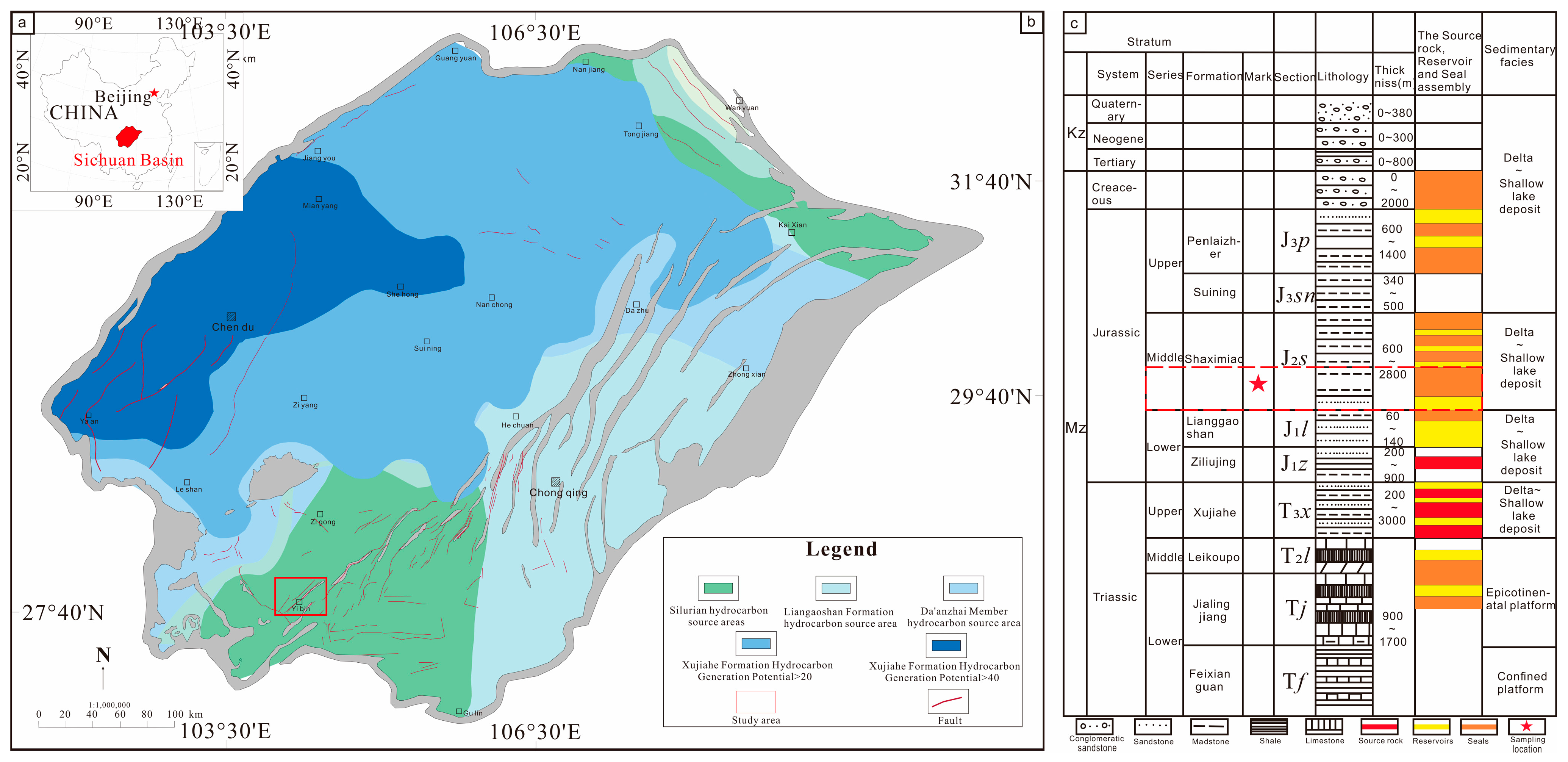
The Sichuan Basin is situated in the western sector of the ancient Yangtze Block and is circumscribed by the Longmen Shan fold belt to the northwest, the Dabashan fault-fold belt to the northeast, the Chuan-Xiang (Sichuan–Hunan) depression-fold belt to the southeast, the Loushan fault-fold belt to the south, and the Emei–Washan block-fault zone to the southwest (Figure 1a,b). It constitutes a multicycle superimposed basin that evolved upon the basement of the Upper Yangtze Craton [22,23,24]. The study area is located in the southwestern part of Sichuan Province, between latitudes 27°40′–27°70′ N and longitudes 103°80′–104°20′ E, occupying a tectonic transition zone between the basin proper and its peripheral orogenic belts [25]. Specifically, it is bordered to the north by the Longmen Shan thrust–nappe belt and the Western Sichuan Depression, to the east by the Central Sichuan paleo-uplift, to the west by the north–south-trending Kangdian Axis structural belt, and to the south by the junction between the Central Sichuan paleo-uplift and the Kangdian Axis. Intense faulting characterizes the region, and episodic uplift of the paleo-high has resulted in localized stratigraphic denudation.
The central Sichuan Basin has undergone a polyphase tectonic evolution spanning the Caledonian, Hercynian, Indosinian, Yanshanian, and Himalayan cycles. Prior to the end of the Middle Triassic, predominantly carbonate-dominated marine successions accumulated, whereas post-Late Triassic strata consist mainly of terrigenous sandstones and mudstones [26,27]. During the late episode of the Indosinian orogeny, the basin transitioned from a foreland to an intracratonic depression, ushering in the Jurassic “red-bed” depositional stage [28] (Figure 1c).
Figure 1. Overview of the study area [27]: (a,b) Location map of the study area within the Sichuan Basin and its surrounding structural belts; (c) Generalized composite stratigraphic column of the Sichuan Basin.
Energies 19 01397 g001
The Shaximiao Formation attains an aggregate thickness of approximately 200 m and is lithologically dominated by red to grayish-green mudstones intercalated with light-gray sandstones. Owing to the paucity of dark mudstones, the formation is organically lean and lacks intrinsic hydrocarbon-generative potential. A regionally persistent conchostracan shale serves as a key marker bed, allowing the Shaximiao Formation to be subdivided into a lower Member I (J2S1) and an upper Member II (J2S2) [29,30]. Provenance analysis indicates that the Shaximiao sediments were primarily supplied by the Dabashan and Micangshan source systems. J2S2 was deposited under semi-arid climatic conditions and is characterized by lobate shallow-water deltas whose individual channel-belt sand bodies are laterally extensive. In contrast, J2S2 accumulated under more arid conditions, typified by dendritic distributary-channel shallow-water deltas; sand bodies are ribbon-like, aligned along narrow, laterally offset and mutually incising channels [31].

3. Data and Methods

3.1. Data Acquisition

A total of 69 wells were used in this study, including 4 cored wells (2 for training, 2 for blind validation) and 65 uncored wells for prediction. This approach ensures that the test data represent entirely new wells, providing a more realistic assessment of the model’s predictive capability in uncored intervals. All machine learning models were implemented in Python 3.8 using the Scikit-learn and TensorFlow libraries. The logging suites employed include natural gamma-ray (GR), spontaneous potential (SP), caliper (CAL), shallow laterolog (LLS), deep laterolog (LLD), acoustic transit time (AC), compensated neutron porosity (CNL), and bulk density (DEN). Supervised Self-Organizing Map (SSOM), Back-Propagation Artificial Neural Network (BPANN), and Gradient-Boosting Decision Tree (GBDT) algorithms were implemented to classify reservoir flow units.

3.2. Data Pre-Processing

Feature scaling is a prerequisite for effective machine-learning classification. Owing to disparate units and dynamic ranges among log curves, raw measurements would otherwise exert disproportionate influence on model convergence and predictive accuracy. To mitigate this, all input curves were subjected to min–max normalization, whereby each curve was linearly rescaled to the interval [0, 1]. Specifically, the minimum value in the training set was mapped to 0 and the maximum to 1. The transformation is defined as
x = x x min x max x min
where x* denotes the normalized value, xmin is the minimum observation in the training set, and xmax is the corresponding maximum. After normalization, all feature values are strictly confined to the interval [0, 1].

3.3. Principles of Machine-Learning Algorithms

3.3.1. Gradient Boosting Decision Tree (GBDT)

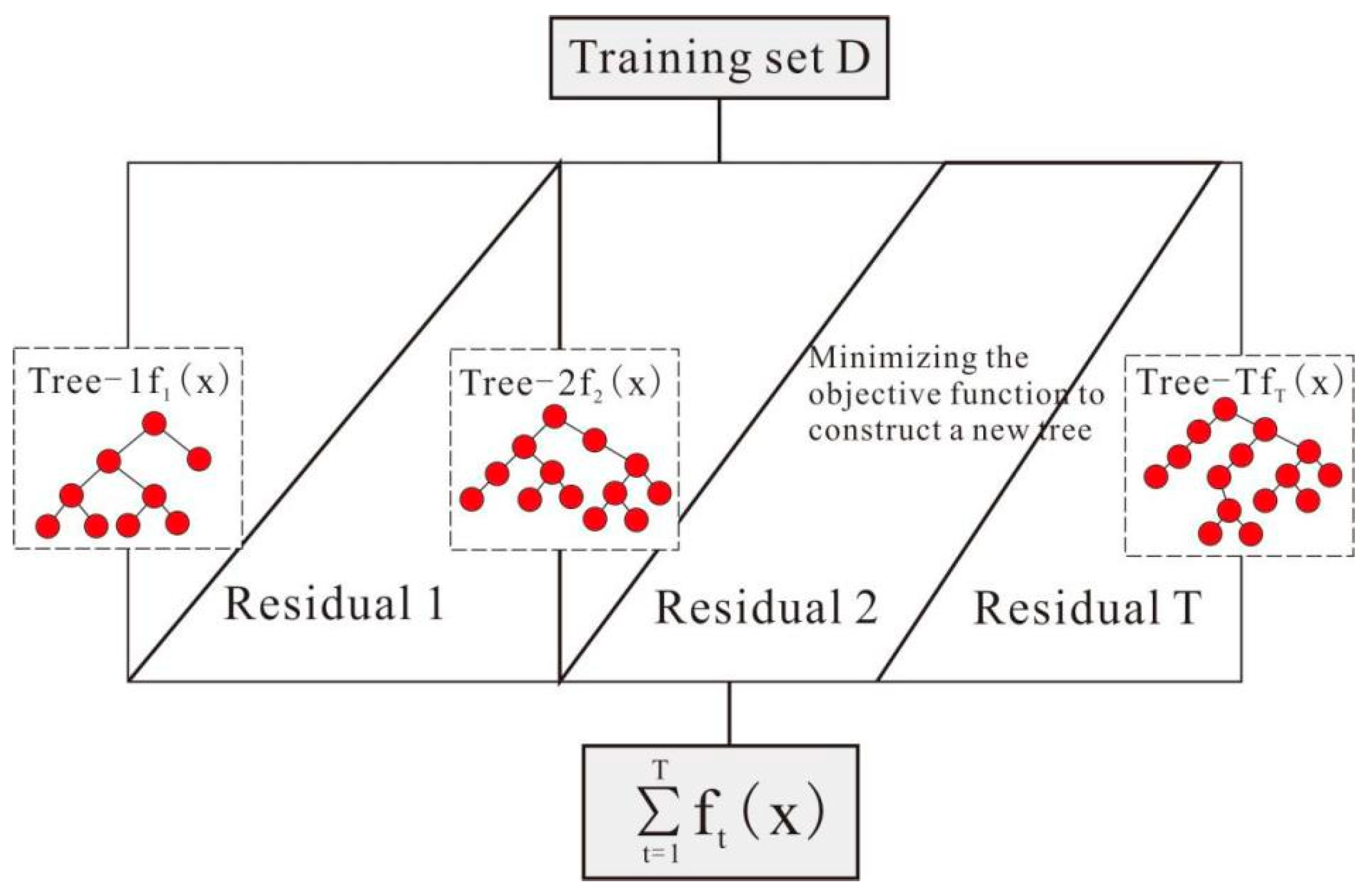
Gradient Boosting Decision Tree (GBDT) is an ensemble learning model renowned for its exceptional predictive capabilities. The core concept involves iteratively training a series of decision trees (weak learners), where each subsequent tree aims to fit the residuals (in regression tasks) or negative gradients (under general loss functions) between the predictions of the previous ensemble and the true values. Through the gradient boosting framework, the model continuously reduces residuals, progressively refining predictions toward the target values. GBDT exhibits remarkable flexibility in handling diverse data types and often achieves high predictive accuracy with relatively minimal parameter tuning. Inheriting the robustness of decision trees against noisy samples, GBDT models maintain this advantage. Furthermore, by adjusting parameters (e.g., the number of trees, tree depth), the model can enhance its ability to capture complex nonlinear relationships in the data, thereby improving generalization performance. Key mechanism: In each iteration, the algorithm calculates the negative gradient of the loss function with respect to the current model’s predictions. This negative gradient serves as the new target for the next weak learner. By fitting to this gradient (an approximation of the residuals), new weak learners are constructed and added to the ensemble. This approach simplifies the optimization of the objective (loss) function. The basic workflow of the GBDT algorithm is illustrated in Figure 2.
The model’s adjustable parameters mainly fall into two categories: boosting framework parameters and weak learner (decision tree) parameters.
Boosting framework parameters: n_estimators: maximum number of iterations (i.e., number of trees). learning_rate: controls each tree’s contribution weight to the final result. loss: the loss function to optimize.
Weak learner parameters: max_depth: maximum depth of decision trees. max_features: maximum number of features considered when splitting nodes. min_samples_leaf: minimum number of samples required at leaf nodes.
Parameter selection is crucial for model performance: An overly small n_estimators value may cause underfitting. An overly small learning_rate may improve precision but significantly slows convergence, requiring larger n_estimators. An overly large max_depth tends to cause overfitting. Therefore, this study uses cross-validation for hyperparameter tuning, with validation-set accuracy as the main evaluation metric. We employ either grid search or random search strategies to find the optimal parameter combination.

3.3.2. The Backpropagation Neural Network Algorithm (BPANN)

Backpropagation Neural Network (BPANN) is a classic type of multilayer feedforward neural network [32,33]. Its core training mechanism consists of two phases:
  • Forward Propagation:
The input signal passes from the input layer through the hidden layer(s), undergoing weighted summation and activation function transformations, and finally reaches the output layer to produce the prediction result.
2.
Backward Propagation:
The error between the network’s predicted output and the true target value is calculated. This error is then propagated backward through the network using the chain rule to update the connection weights and thresholds (biases) between neurons in each layer.
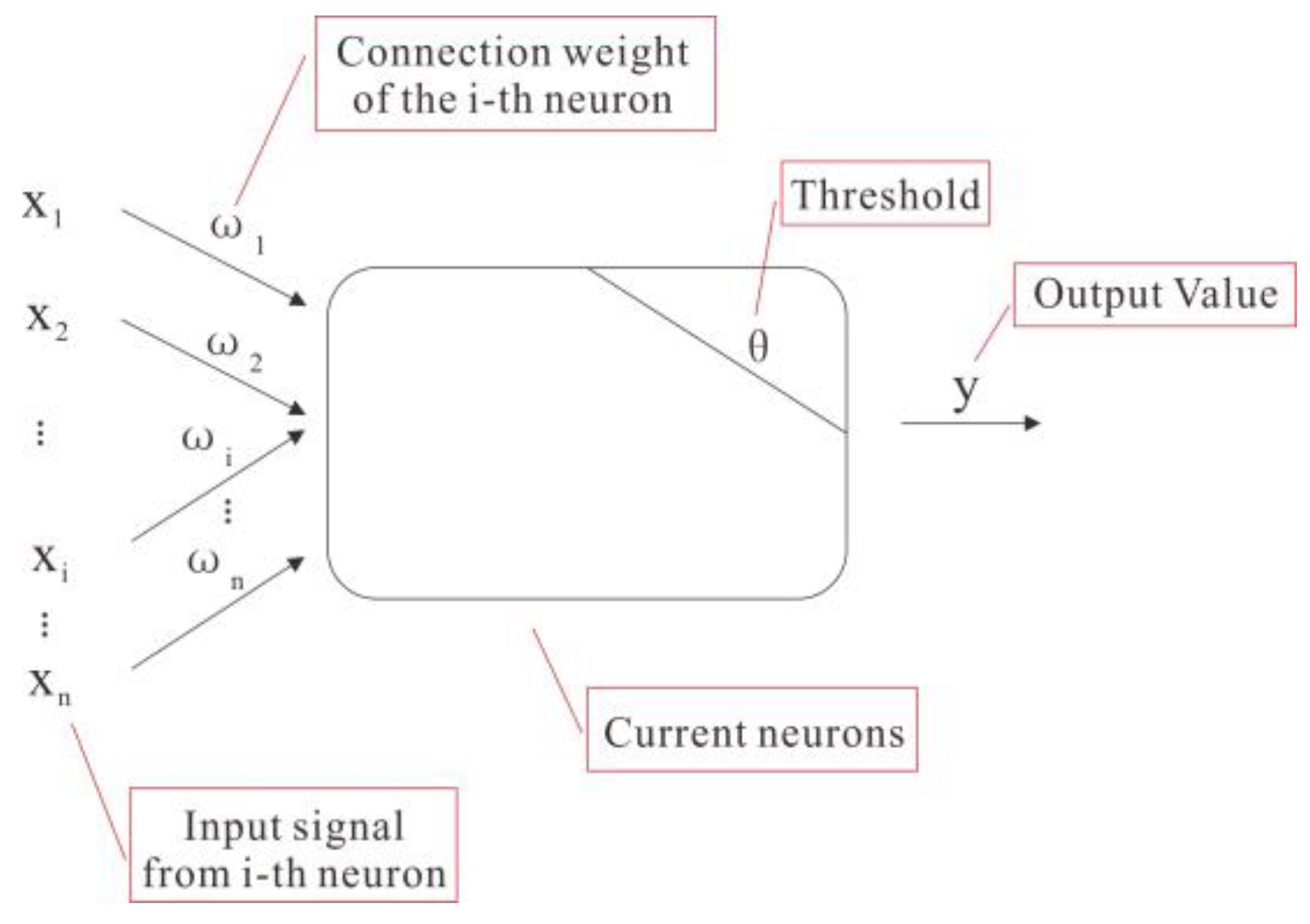
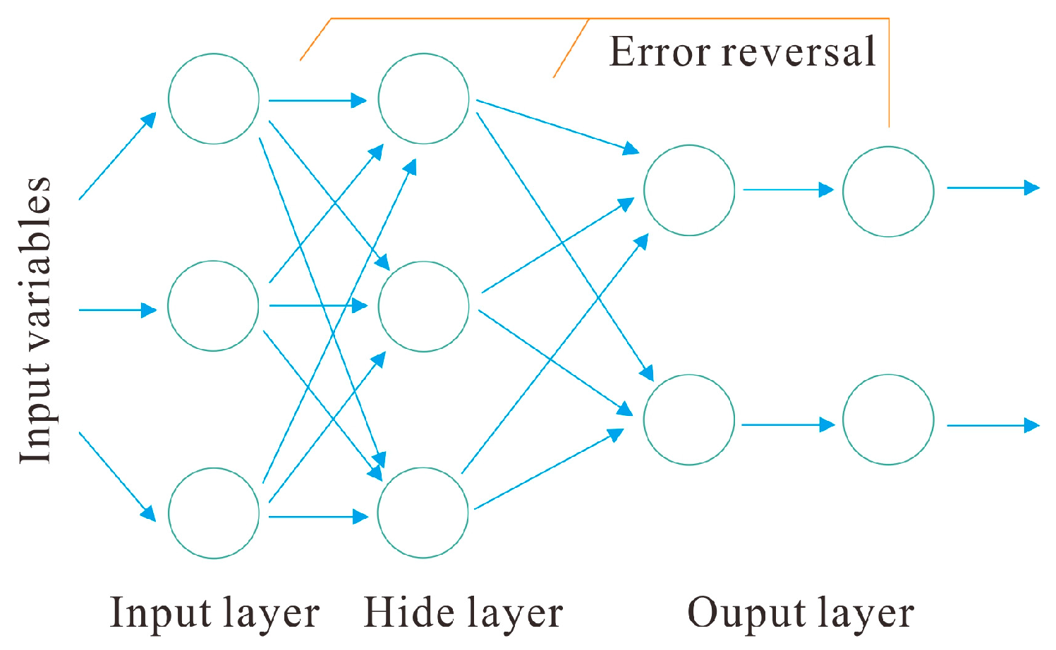
The BP algorithm aims to minimize the network’s output error (typically defined as Mean Squared Error, MSE) as the objective function. It employs Gradient Descent to iteratively adjust the network parameters (weights and biases), continuously reducing the objective function value until convergence is achieved. A schematic diagram of a typical neural network structure is shown in Figure 3. Each component of the structure has its specific function: The input layer is primarily responsible for receiving external input information. The output layer serves as the final output of the processed results. The hidden layer(s), located between the input and output layers, play the most crucial role by processing the input information received from the input layer. We adopt the classic and essential Backpropagation (BP) neural network model, a type of feedforward network, to establish a production capacity prediction model. The BP neural network model operates based on two key principles: forward data transmission and error feedback correction, as illustrated in Figure 4.
During the forward propagation process in Figure 4, the input signals from other neurons enter the neuron structure, where they undergo weighted summation and threshold-based computation. The resulting output is then passed to the hidden layer. Neurons in the hidden layer repeat this computation and transmit the processed variables to the next layer—the output layer. At this point, the forward propagation phase is largely completed. Upon receiving the transmitted signals, the input layer compares the expected output value with the computed output value. The calculated error is then propagated backward to the input layer, allowing continuous adjustment of the weights and thresholds in the output layer. This cycle repeats iteratively. During this iterative process, once the computed error falls below the predefined expected error threshold set during model establishment, the loop terminates, and the final result is output. This completes the error backpropagation and correction process.

3.3.3. Supervised Self-Organizing Map Neural Network Algorithm (SSOM)

The Self-Organizing Map (SOM) neural network algorithm, proposed by Kohonen in 1982 [34], is an unsupervised clustering analysis algorithm consisting of a two-layer neural network structure: the input layer and the competitive layer (Figure 5a). The number of nodes in the input layer corresponds to the dimensionality of the input flow unit samples. When receiving input features from flow unit samples, neurons in the competitive layer compete to respond to the input pattern. Ultimately, the winning neuron is activated, while the losing neurons are suppressed, and the winning neuron represents the classified flow unit of the input sample.
The SOM algorithm has achieved good application results in lithology identification, fluid prediction, and remote-sensing image classification [35,36]. However, when dealing with pattern classification problems involving strong nonlinear relationships, it suffers from limitations such as low classification accuracy, difficulties in sample statistics, and challenges in extracting non-significant information [36]. To address these issues, researchers have proposed an improved supervised version called the Supervised Self-Organizing Neural Network (SSOM) algorithm [37].
Compared with the SOM algorithm, the SSOM algorithm incorporates an additional output layer, and its neural network structure is illustrated in Figure 5b. During the supervised learning and training process, weight correction between the competitive layer and the input/output layers is achieved by adjusting the weights of all neurons in the neighborhood of the winning node. The core principle of this algorithm is to modify the weights by analyzing the consistency between the predicted flow unit categories (from input samples) and the flow unit categories determined by core analysis. This process helps establish a flow unit prediction model, enabling the prediction of flow units in uncored wells.

3.4. Model Training and Hyperparameter Tuning

To ensure reproducibility, all models were trained using a well-based cross-validation strategy. The training set (wells W1 and W2) was further split, with one well used for internal validation during hyperparameter tuning.
SSOM: The SSOM network was trained with a competitive layer of 10 × 10 neurons. The training used a batch training algorithm with 200 epochs. The initial learning rate was set to 0.5 and decreased linearly over epochs. Neighborhood radius started at 3 and decreased to 1. Supervised learning commenced after 50 unsupervised pre-training epochs to initialize the map. The final model was selected based on the lowest quantization and topographic errors on the validation well.
BPANN: A three-layer network (8 input, 15 hidden, 5 output neurons) was built. The hidden layer used a sigmoid activation function, and the output layer used softmax. Training employed the Adam optimizer with a learning rate of 0.001, mini-batch size of 16, and a maximum of 500 epochs. Early stopping with a patience of 20 epochs was used to prevent overfitting, monitoring the loss on the validation well.
GBDT: The GBDT model was tuned using a grid search with 5-fold cross-validation on the training well. The optimal parameters found were: n_estimators = 150, learning_rate = 0.1, max_depth = 5, min_samples_leaf = 5. The deviance loss function was used for classification.
Additional Algorithms (for comparison): For a broader comparison, we also implemented a Random Forest (RF) classifier, an XGBoost classifier, and a Linear Support Vector Machine (Linear SVM) as a baseline. These were trained and validated using the same well-based split and tuning protocols. Hyperparameters for RF (e.g., n_estimators = 200, max_depth = 6) and XGBoost (e.g., n_estimators = 150, learning_rate = 0.1, max_depth = 4) were also optimized via grid search.

3.5. Flow Unit Division Methods

This study adopted the Flow Zone Indicator (FZI) method for reservoir flow unit classification. Proposed by [38], this method utilizes reservoir rock effective porosity (φe) and permeability (K) data to calculate FZI values that characterize pore-throat structural features, thereby grouping rocks with similar flow characteristics into identical flow units.
The calculation of FZI values is based on the following key parameters:
Reservoir Quality Index (RQI):
R Q I = 0.314 k φ e
where:
K = permeability (in millidarcies, mD)
φ = porosity (in %)
Normalized porosity (φz):
φ z = φ e 1 φ e
Flow Zone Indicator (FZI):
FZI = RQI/φz
Classification principle: On a log-log plot (log(RQI) versus log(φz)), samples with identical FZI values will align along a straight line with a slope of 1. Therefore, by determining the distribution range of FZI values (typically identified through truncation points on the cumulative probability distribution curve of FZI values), the reservoir can be divided into several flow unit types with distinct flow capacities (e.g., Class I, II, III, and IV). In this study, in addition to conventional porosity–permeability controlled flow units, we specifically identified fractured flow units (see Section 4.3.1 for results).

4. Results

4.1. Reservoir Characteristics

4.1.1. Petrological Characteristics

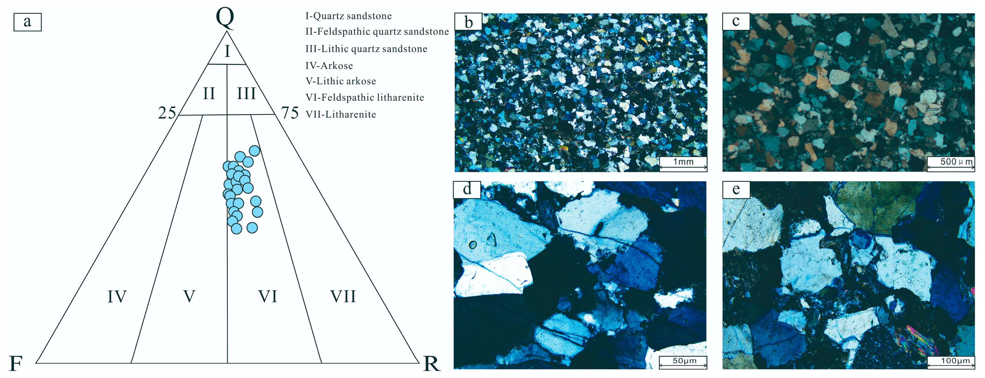
Before the deposition of the Shaximiao Formation in the Sichuan Basin, the region constituted a broad eastward-dipping ramp; the Longmen Shan area lay to the west as the dominant sediment source, whereas the Micang–Daba Mountains supplied detritus from the north. Detritus from the Longmen Shan provenance is characterized by high quartz and low feldspar contents, whereas the Micang–Daba source yields low-quartz, high-feldspar assemblages. In the Yibin area, the second sub-member of the Shaximiao Formation (J2S1) is strongly influenced by the Micang–Daba provenance, and is dominated by feldspathic lithic arenites with minor feldspathic sandstones; microfractures are well developed. Plagioclase and K-feldspar are the common feldspar varieties, and monocrystalline quartz is abundant among the quartz grains. Rock fragments are rich in metamorphic types and moderately abundant in magmatic types. Intergranular matrix consists chiefly of clay minerals with minor chlorite; cements are dominated by calcite accompanied by minor quartz overgrowths (Figure 6). Grain contacts are dominantly point or tangential, indicating contact cementation. Grains are poorly rounded and moderately sorted.

4.1.2. Physical Properties

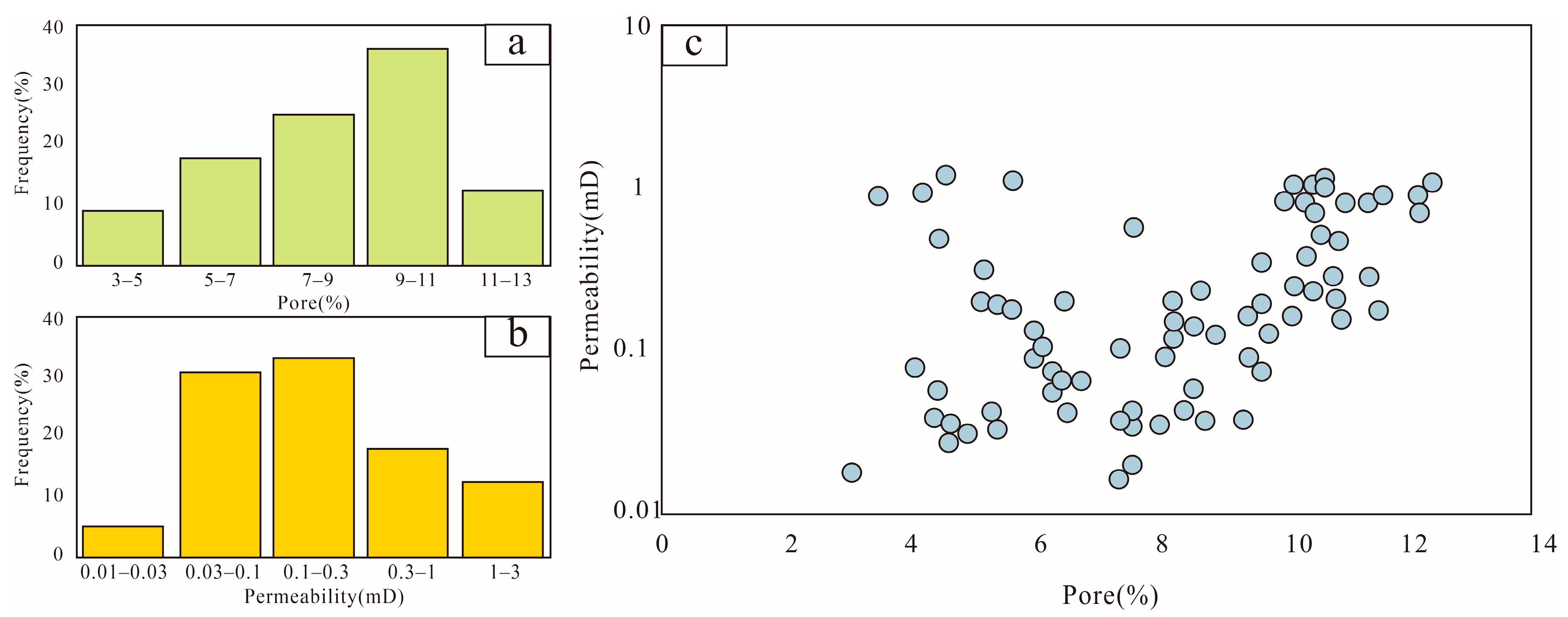
The physical properties of tight sandstones in the Sha-1 Member (J2s1) of the Shaximiao Formation in the study area show that the porosity ranges from 3.1% to 12.7%, with an average of 8.6% and a peak value in the range of 9–11% (Figure 7a). The permeability varies from 0.02 × 10⁻³ μm2 to 2.78 × 10⁻³ μm2, with an average of 0.45 × 10⁻³ μm2 and a median of 0.18 × 10⁻³ μm2, and its peak value falls in the interval of 0.1–0.3 × 10⁻³ μm2 (Figure 7b).
The samples are classified as low-porosity, low-permeability sandstone reservoirs. Porosity–permeability cross-plot (Figure 7c) shows a general positive correlation, consistent with typical tight reservoirs. Anomalous Samples: Some samples exhibit low porosity but relatively high permeability, attributed to developed microfracture networks that enhance matrix flow capacity.

4.2. Characteristics of Reservoir Pore Structure

4.2.1. Pore Types in Reservoir Rocks

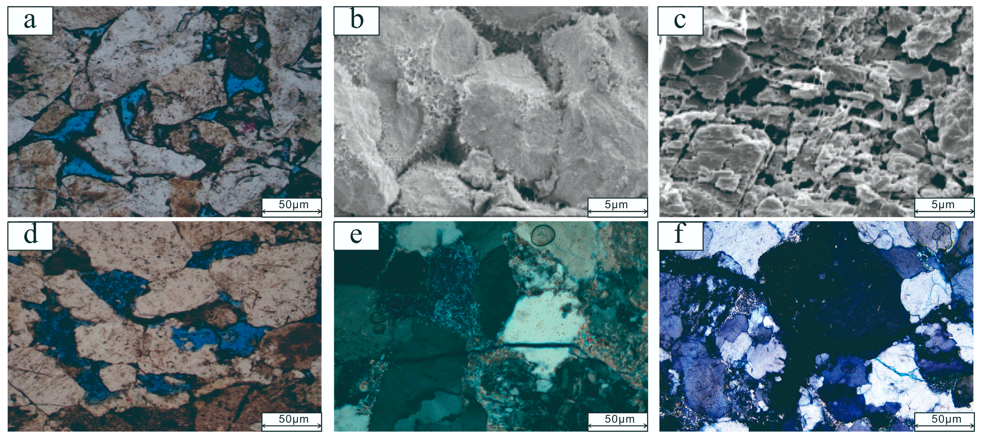
Integrated SEM and cast thin-section analyses demonstrate that residual intergranular pores (1.5–5.7% by volume, Figure 8a,b) and feldspar dissolution pores (0.1–2.5% by volume, Figure 8c,d) constitute the predominant reservoir spaces in the Sha-1 Member (J2S1) of the study area, with well-developed microfractures (Figure 8e,f). The dissolution-intergranular pore assemblage represents the dominant pore type combination.

4.2.2. Classification of Pore Throats and Pore Structure

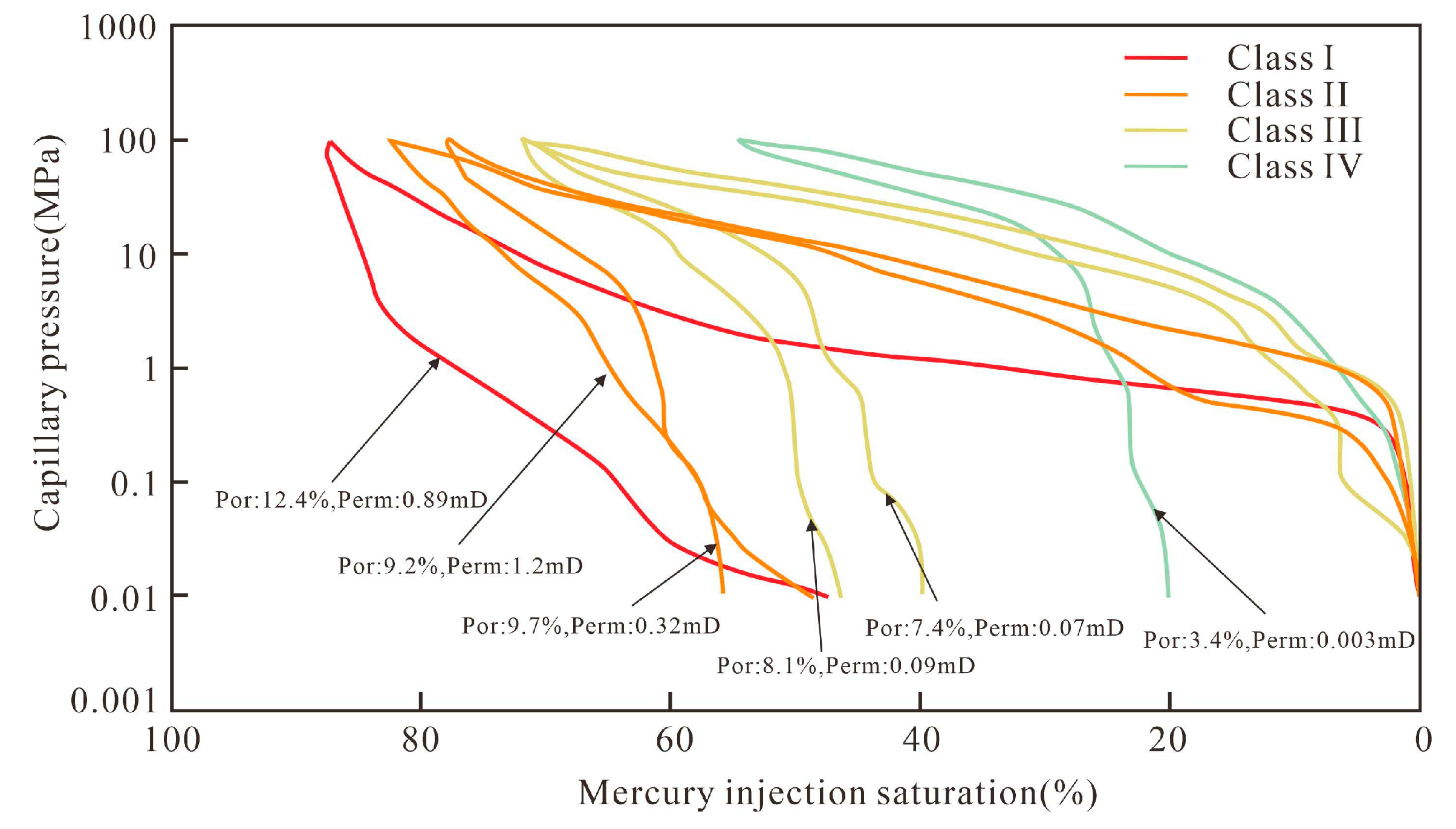
Mercury-injection parameters commonly used to characterize the pore structure of low-permeability sandstone reservoirs include the maximum pore-throat radius (Rmax), threshold pressure (pd), median pressure (p50), median pore-throat radius (R50), sorting coefficient (C), maximum mercury saturation (Smm), and mercury withdrawal efficiency (Emr). Capillary-pressure statistics for the J2S1 samples show that pd averages 0.79 MPa, Rmax averages 1.87 μm, and Smm averages 87.14%. Overall, the J2S1 reservoir in the study area is characterized by fine throats, high threshold pressures, and small median pore-throat radii, all typical of ultra-low-permeability reservoirs.
Based on pore-structure quality, the non-fractured intervals of the J1S1 reservoir can be divided into four classes. Class I is the most favorable, typified by large pores and coarse throats with pd < 1 MPa, whereas Class IV is the poorest, represented by medium pores and fine throats with pd generally >10 MPa (Figure 9).

4.3. Identification of Reservoir Flow Units

4.3.1. Reservoir Flow Unit Division

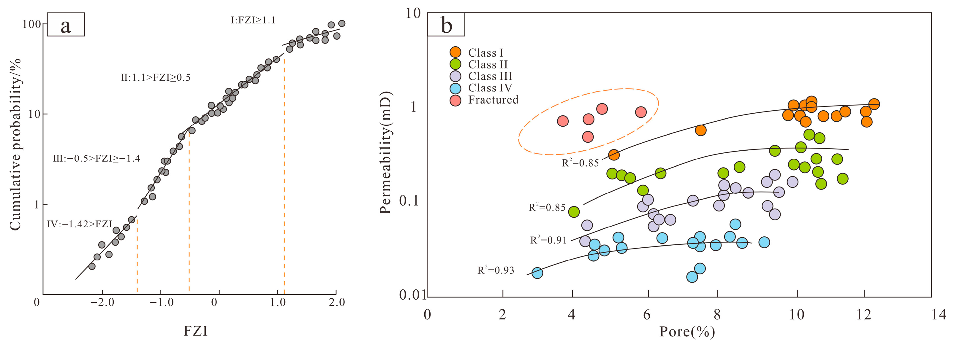
Based on petrophysical data from 85 non-fractured tight sandstone samples in the study area, flow units were classified using the Flow Zone Indicator (FZI) method.
Four major FZI intervals were identified as boundaries for conventional flow unit division based on the cumulative probability distribution of FZI values (Figure 10a).
Considering the significant influence of fractures on flow, samples exhibiting low porosity (average 4.4%) but high permeability (average 0.85 mD) were separately classified as fracture-type flow units.
Ultimately, the Sha-1 Member reservoir was divided into five flow unit types (I, II, III, IV, and fracture-type), with detailed petrophysical parameters, FZI ranges, and production characteristics shown in Table 1 and (Figure 10b).
The characteristics of different flow unit types vary significantly:
Class I units show the best reservoir quality (average porosity 10.7%, average permeability 0.675 mD), with FZI > 1.1 corresponding to Type I/II pore structures, and the highest average daily gas production (40,700 m3/d).
Class II units demonstrate good properties (average porosity 8.9%, average permeability 0.37 mD), with FZI between −0.6–1.1 and relatively high productivity (average 31,200 m3/d).
Class III units exhibit medium-poor quality (average porosity 7.5%, average permeability 0.09 mD), with FZI between −1.5–0.6 and significantly reduced productivity (average 7700 m3/d).
Class IV units show the worst properties (average porosity 5.3%, average permeability 0.035 mD), with FZI < −1.5 and minimal productivity (average 2400 m3/d).
Considering the significant influence of fractures on flow, samples were classified as fracture-type flow units based on a combined interpretation of multiple lines of evidence: Production Anomaly: Samples exhibiting low porosity (average 4.4%) but permeability > 0.5 mD, which is significantly higher than the matrix permeability expected for rocks with such low porosity based on the porosity–permeability trend for non-fractured samples (Figure 10b). The specific threshold of >0.5 mD was chosen as it represents a permeability value exceeding the 90th percentile for rocks with porosity < 6% in the non-fractured dataset.
Sensitivity Analysis: The classification of fracture-type units is most sensitive to the chosen permeability threshold. To assess this, we tested thresholds of 0.4 mD and 0.6 mD. A lower threshold (0.4 mD) increased the number of fracture-type samples by 12%, introducing samples with only minor, less-conductive fractures, which slightly lowered the average permeability of the class to 0.73 mD and reduced its average production to 12,100 m3/d. A higher threshold (0.6 mD) excluded some samples with clear core-scale fractures but lower effective conductivity, reducing the class size by 18% but raising its average permeability to 0.98 mD and production to 15,800 m3/d. The chosen threshold of 0.5 mD provided the most balanced representation, aligning best with core descriptions and production characteristics. Ultimately, 12 samples met these combined criteria and were labeled as fracture-type units.

4.3.2. Intelligent Identification of Flow Units Based on Machine Learning Algorithms

To establish a quantitative well-log identification model for flow units, 142 core-analyzed flow unit samples (covering the aforementioned 5 types) were used. The dataset was strictly divided based on wells into a training set (100 samples from wells W1 and W2) and an independent blind test set (42 samples from wells W3 and W4). Three machine learning algorithms—SSOM, BPANN, and GBDT—were applied for model training and testing. The results reported below are based on the performance of the trained models on these completely unseen wells. Input well logs included GR, SP, CAL, LLS, LLD, AC, CNL, and DEN, with three machine learning algorithms—SSOM, BPANN, and GBDT—applied for model training and testing.
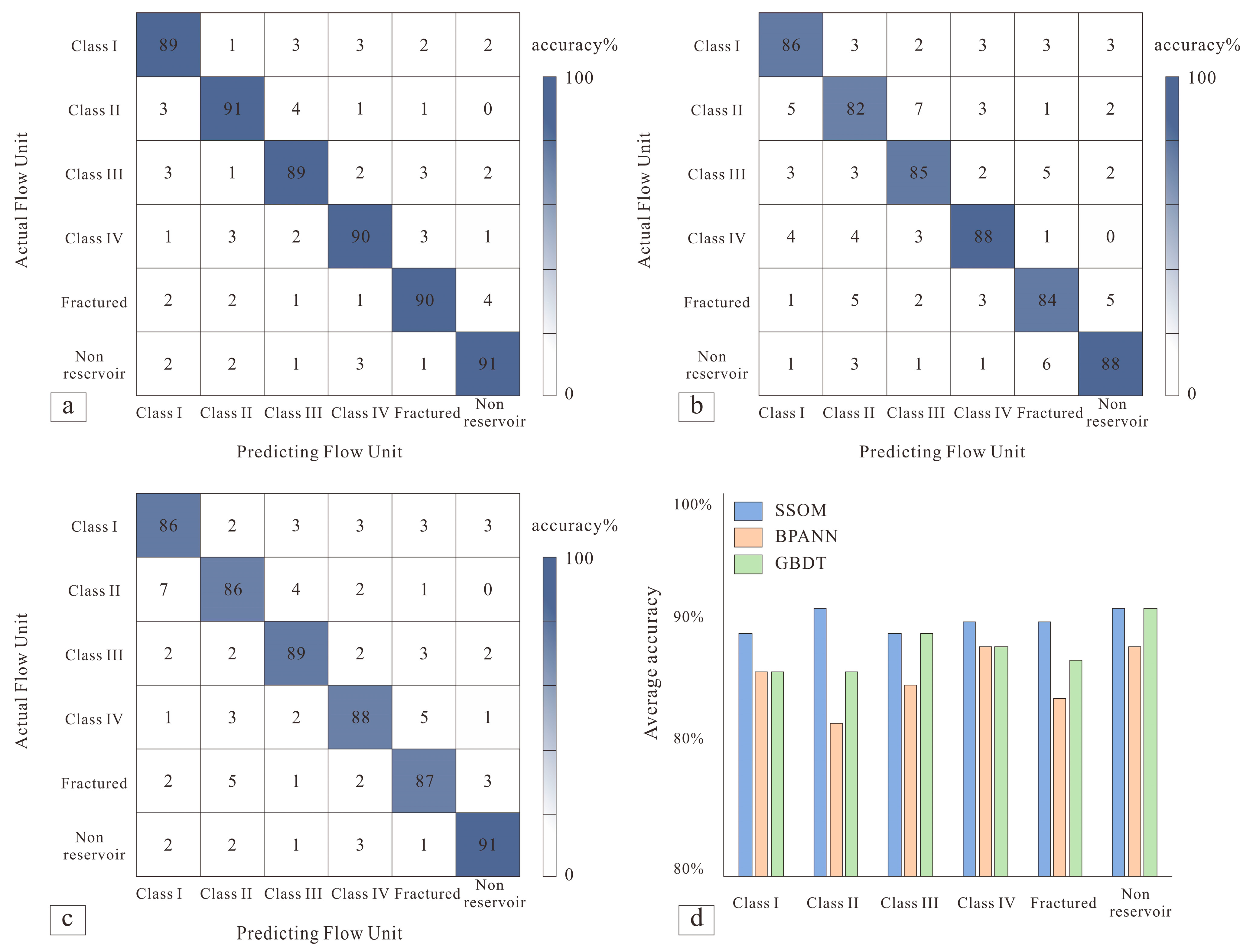
Results of flow unit identification based on the SSOM algorithm showed high accuracy for all flow unit types, with an average accuracy of approximately 90.1%. The BPANN algorithm achieved an average accuracy of about 85.5%, while the GBDT algorithm yielded an average accuracy of around 87.8% (Figure 11a–c). The SSOM algorithm demonstrated superior performance across all metrics. It achieved the highest macro-average F1-score of 0.89, significantly outperforming GBDT (0.82) and BPANN (0.80). Critically, for the fracture-type flow unit—a minority class representing only 7% of training samples—SSOM achieved a recall of 0.83 and an F1-score of 0.80, indicating its robustness in identifying these critical, high-permeability zones. In contrast, GBDT and BPANN showed much poorer performance on this class, with F1-scores of 0.50 and 0.44, respectively, primarily due to low recall (Figure 11b,c). This highlights SSOM’s unique capability in decoupling the nonlinear well-log responses of fractured reservoirs, even with limited training examples. Detailed per-class performance metrics for all three algorithms are summarized in Table 2.
A comparison of the three algorithms’ prediction results was conducted to analyze their respective applicability. Each algorithm has its own advantages, disadvantages, and suitable application conditions. The SSOM algorithm optimizes samples through neural network training, with the advantages of good stability and the ability to differentially process imbalanced training data during the training process. This enables the established model to provide accurate judgments when identifying similar prediction samples, eliminating the need for data augmentation. It effectively captures the nonlinear relationship between fractured reservoirs and well-log parameters and demonstrates relatively high accuracy in predicting flow unit types with fewer samples or higher class-domain overlap. While both BPANN and GBDT algorithms generally achieve high accuracy, their performance is relatively poorer for flow unit types with fewer samples or higher class-domain overlap.
In summary, the advantages of the SSOM algorithm are: (1) good stability: It can effectively handle class imbalance problems; (2) capturing complex nonlinear relationships: It shows outstanding capability in identifying well-log response patterns of fractured reservoirs; (3) high-resolution identification: Its recognition accuracy for flow unit types with limited samples or high class-domain overlap (e.g., Class III/IV boundaries) is significantly better than that of BPANN and GBDT (Figure 11d).
In addition to the three primary algorithms, the performance of Random Forest (RF), XGBoost, and a linear baseline (Linear SVM) was evaluated on the same blind test wells (Table 3). The SSOM algorithm (90.1% accuracy, macro F1 0.89) continued to outperform these models. XGBoost (88.5% accuracy, macro F1 0.84) and RF (87.9% accuracy, macro F1 0.83) performed better than GBDT and BPANN but still lagged behind SSOM, particularly in identifying the fracture-type units (F1-scores of 0.62 and 0.58, respectively). The Linear SVM baseline achieved only 72.4% accuracy (macro F1 0.65), confirming the necessity of using non-linear models to capture the complex relationships in the data.
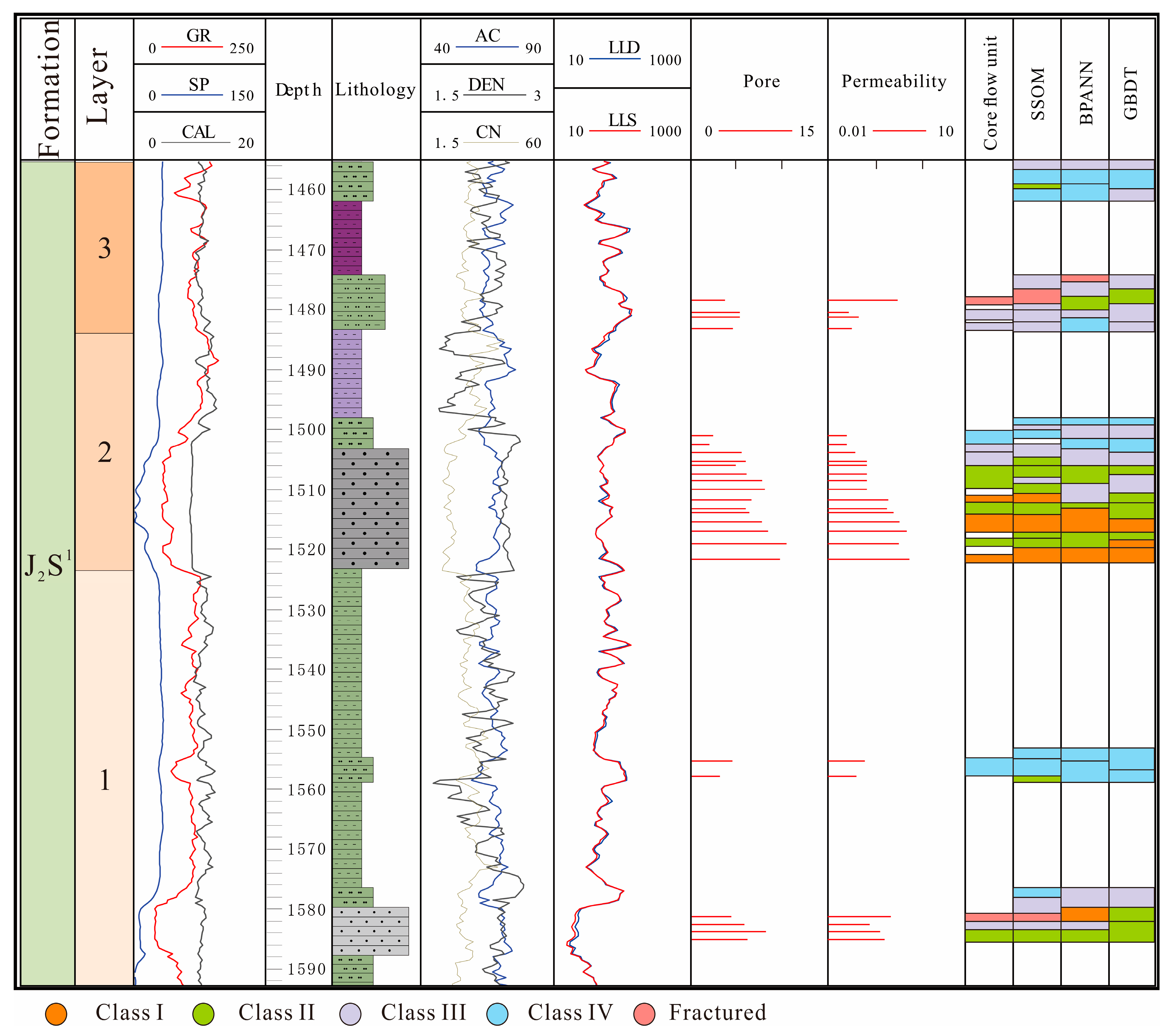
Comprehensive histogram analysis further confirms that the SSOM algorithm not only effectively identifies complex flow unit architectures within sand bodies, but also clearly reveals the vertical cyclicity of flow unit types in channel sandstones (showing gradual improvement in flow unit quality from base to top). This provides a more refined perspective for characterizing reservoir heterogeneity (Figure 12).

5. Discussion

Based on the identification results of flow units in uncored intervals of the J2S1 member using the SSOM model, integrated with analyses of sedimentary facies, tectonic setting, and reservoir characteristics, this section focuses on discussing the spatial distribution patterns and controlling factors of flow units in the Shaximiao Formation reservoirs.

5.1. Vertical Development Characteristics of Reservoir Flow Units

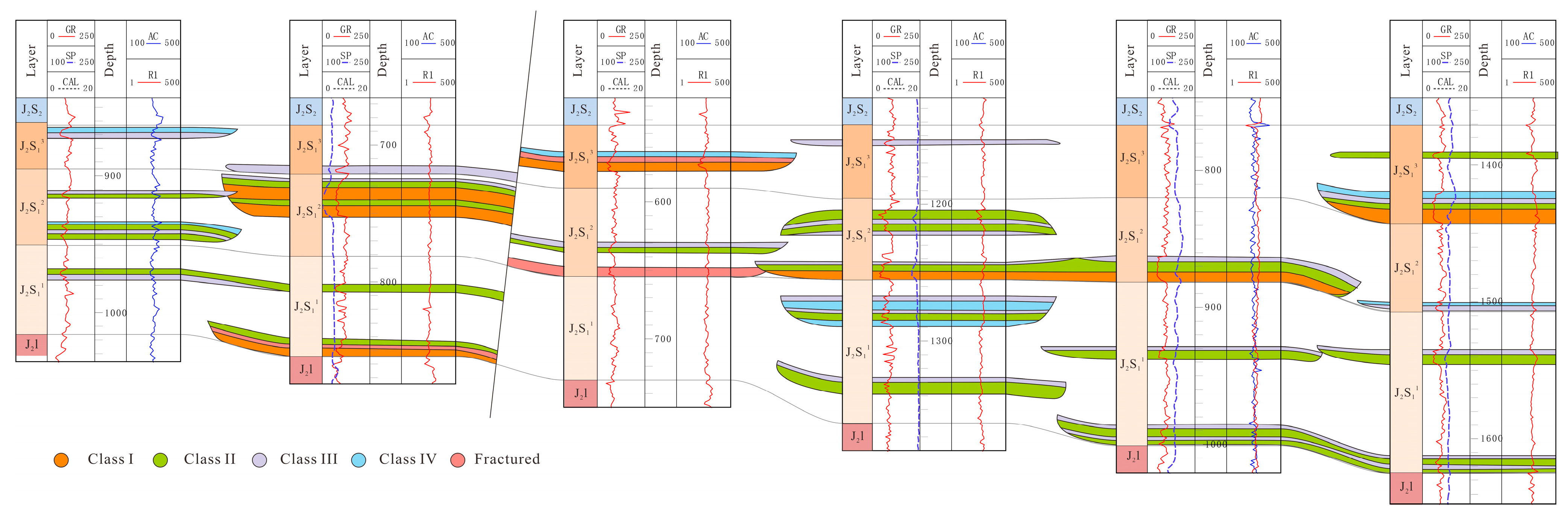
The vertical distribution of flow units in the J2S1 Member of the Shaximiao Formation is significantly controlled by sedimentary facies evolution (Figure 13).
The J2S11 sub-member belongs to a delta front subfacies, mainly developing multi-stage stacked subaqueous distributary-channel sand bodies. The individual sand layers are relatively thin with moderate lateral continuity. Influenced by depositional hydrodynamics and subsequent diagenetic alteration, flow units in this interval are predominantly Class II, reflecting moderate flow capacity.
The J2S12 sub-member is primarily a delta plain subfacies, developing 2–3 stages of main distributary-channel deposits. The sand bodies are thick with generally good reservoir quality. Due to lag deposits or strong hydrodynamic scouring, the channel bases often develop Class I flow units with the best physical properties, while the middle to upper parts of channels are mainly composed of Class I or II units.
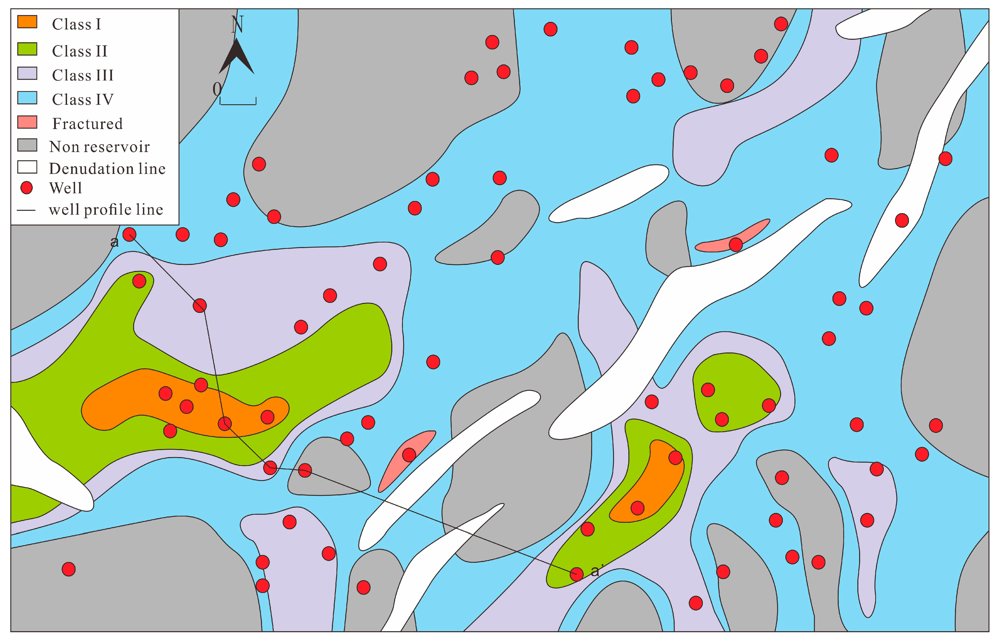
The J2S13 sub-member transitions back to a delta front subfacies, developing 1–2 stages of subaqueous distributary channels. The sand body thickness varies greatly with poor continuity. Flow units are mainly Class II–III. Notably, fracture-type flow units are significantly enriched in this sub-member and are predominantly distributed near faults (Figure 13), indicating that tectonic activity (faulting) is the key factor inducing fracture development and forming dominant flow.

5.2. Planar Development Characteristics of Reservoir Flow Units

The planar distribution pattern of flow units in the J2S13 sub-member is the result of combined effects from sedimentary facies distribution and later tectonic modification (Figure 14). The distribution inherits the paleogeographic framework, with channel sand bodies showing a ribbon-shaped distribution. Influenced by the sediment source direction from the Micang Mountains, high-quality reservoir sands (mainly developing Class I and II flow units) are predominantly concentrated in the southern and southwestern parts of the study area (proximal to the source), but appear as localized ribbon-shaped distributions with poor lateral continuity. In areas farther from the source (northern and northeastern parts), sand bodies become thinner with poorer physical properties, where Class IV flow units are extensively distributed, becoming the dominant type across the plane.
The key role of tectonic fracture control is evident as fracture-type flow units are not uniformly distributed but highly enriched near major faults (within ≤2 km distance) or paleo-uplift denudation lines (Figure 14). These structurally active zones with concentrated stress have induced the development of microfracture networks, significantly improving local reservoir flow capacity and creating special high-permeability zones distinct from conventional porosity–permeability-controlled areas.
The combination of sedimentary facies differentiation and localized tectonic fracture modification results in extremely strong heterogeneity in the planar distribution of flow units within the J2S13 sub-member. Different types of units are interwoven spatially, showing significant variations in flow capacity. This heterogeneity has crucial implications for development-well pattern design and stimulation strategy selection.
The findings from the Shaximiao Formation can be contextualized by comparing them with other tight sandstone reservoirs globally. For instance, in the Upper Cretaceous Abu Roash-A sandstone reservoir in the Beni Suef Basin, Western Desert of Egypt [39], also employed hydraulic flow unit (HFU) analysis to characterize reservoir heterogeneity. While the Beni Suef reservoir exhibits higher porosity (20–24%) compared to the Shaximiao Formation (<12%), it displays similar permeability anisotropy and strong facies control on flow quality. In both cases, the Flow Zone Indicator (FZI) method effectively differentiated high- and low-quality flow units. However, a key distinction in our study is the explicit identification and modeling of fracture-type flow units, which are crucial for productivity in the ultra-low permeability matrix of the Shaximiao Formation. In the Beni Suef example, fractures are not reported as a primary control, and the permeability is dominated by matrix properties (<20 mD). This comparison highlights that while the FZI method is a robust tool for characterizing matrix heterogeneity, reservoirs in complex structural settings, like the southern Sichuan Basin, require an integrated approach that also accounts for tectonically-induced fracture networks to fully capture the range of flow behaviors.

6. Conclusions

Through multidisciplinary integration, this study has achieved the following innovative findings:
(1)
By overcoming the limitations of traditional FZI methods and incorporating fracture flow effects, we established a five-dimensional flow unit classification standard (“four conventional types + fracture-type”). The fracture-type units, characterized by low porosity (4.4%) and high permeability (0.85 mD), demonstrate an average daily gas production of 14,200 cubic meters, serving as key contributors to high productivity in low-porosity reservoirs.
(2)
The study confirmed the superiority of the SSOM algorithm in identifying flow units in complex reservoirs, with its 90.1% prediction accuracy stemming from its capability to decouple high-dimensional nonlinear relationships (particularly fracture responses), providing a reliable tool for predicting units in uncored intervals.
(3)
Vertically, the differentiation of flow units is controlled by depositional sequences—Class I units predominantly develop at the base of delta plain channels (J2S12), while delta front thin sand bodies (J2S11/3) are mainly composed of Class II units. Horizontally, the coupling of tectonic and depositional processes results in strong heterogeneity, with high-quality units (Class I/II) showing ribbon-like distributions near sediment sources and fracture-type units being enriched along fault zones.

Author Contributions

Conceptualization, H.Y. and H.L.; Methodology, J.L. and Y.D.; Data curation, Z.Z. and L.J.; Writing—original draft, X.W.; Writing—review & editing, L.Z. All authors have read and agreed to the published version of the manuscript.

Funding

This research was funded by the Science and Technology Research Project of Chongqing Education Commission grant number No. KJZD-K202401503.

Data Availability Statement

All relevant data are contained within the paper.

Conflicts of Interest

Authors H.Y.; J.L.; Y.D.; Z.Z.; L.J.; and H.L. were employed by the company Shunan Division, PetroChina Southwest Oil & Gasfield Company. The remaining authors declare that the research was conducted in the absence of any commercial or financial relationships that could be construed as a potential conflict of interest.

References

  1. Zou, C.-N.; Zhu, R.-K.; Bai, B.; Yang, Z.; Hou, L.-H.; Zha, M.; Fu, J.-H.; Shao, Y.; Liu, K.-Y. Significance, geologic characteristics, resource potential and future challenges of tight oil and shale oil. Bull Miner. Petrol. Geochem. 2015, 34, 3–17. [Google Scholar]
  2. Cai, Y.-D.; Gao, G.-S.; Liu, D.-M.; Qiu, F. Geological conditions for coal measure gas enrichment and accumulation models in Linxingzhong block along the eastern margin of the Ordos Basin. Nat. Gas Ind. 2022, 42, 25–36. [Google Scholar]
  3. Guo, T.-L.; Xiong, L.; Ye, S.-J.; Dong, X.-X.; Wei, L.-M.; Yang, Y.-T. Theory and practice of unconventional gas exploration in carrier beds: Insight from the breakthrough of new type of shale gas and tight gas in Sichuan Basin, SW China. Pet. Explor. Dev. 2023, 50, 24–37. [Google Scholar] [CrossRef] [Scilit]
  4. Mao, J.-B.; Yan, W.-L.; Fei, H.-Y.; Chen, W.-D.; Fei, Z.Q. Reservoir characteristics of Shaximiao Formation in Wubaochang structure, northeastern Sichuan Basin. Nat. Gas Ind. 2007, 27, 8–10. [Google Scholar]
  5. Ye, J.-L.; Li, Z.-Q.; Zhang, Y. On the genesis of fissures in the Shaximiao Formation, Wubaochang. Acta Geol. Sichuan 2011, 31, 162–166. [Google Scholar]
  6. Wang, X.-J.; Chen, S.-L.; Xie, J.-R.; Ma, H.-L.; Zhu, D.-Y.; Pang, X.-T.; Yang, T.; Lv, X.-Y. Accumulation characteristics and main controlling factors of tight sandstone of Jurassic Shaximiao Formation in southwestern Sichuan Basin. Lithol. Reserv. 2024, 36, 78–87. [Google Scholar]
  7. Guo, J.-L.; Jia, C.-Y.; Yan, H.-J.; Ji, L.-D.; Li, Y.-L.; Yuan, H. Research methodology and application of reservoir permeability units for tight sandstone gas reservoirs: A case study in the Permian Lower Shihezi Formation of the Ordos Basin. Geol. J. China Univ. 2018, 24, 412–424. [Google Scholar]
  8. Hearn, C.L.; Ebanks, W.J.; Tye, R.S.; Ranganathan, V. Geological factors influencing reservoir performance of the Hartzog Draw Field, Wyoming. J. Pet. Technol. 1984, 36, 1335–1344. [Google Scholar] [CrossRef] [Scilit]
  9. Yuan, B.-L.; Zhang, H.; Ye, Q.; Zhang, L.-Z.; Chen, Z.-H.; Chao, C.-X.; Dong, D.-X.; Huan, J.-L. Flow-unit classification based on compound sand-body architecture of delta and distribution pattern of remaining oil. Acta Sedimentol. Sin. 2021, 39, 1253–1263. [Google Scholar]
  10. Liu, R.-H.; Sun, Y.; Yan, B.-Q.; Zhang, Y.-G.; Huang, Y.-S.; Wang, N.; Wang, X.-R. Reservoir flow units for dynamic and static combinations: Case study of Neogene Guantao Formation in block M, Gudao Oilfield. Acta Sedimentol. Sin. 2023, 41, 1170–1180. [Google Scholar]
  11. Yuan, C.-P.; Yao, G.-Q.; Xu, S.-H.; Zhou, F.-D. Review on fluid flow unit in oiland gas reservoirs. Geol. Sci. Technol. Inf. 2006, 25, 23–28. [Google Scholar]
  12. Feng, X.-H.; Liu, X.-F.; Yue, Q.-S.; He, J.-S. A new method for heterogeneity description of thick reservoir: Hydraulic flow units analysis. Acta Petrolei Sin. 1994, 15, 149–158. [Google Scholar]
  13. Fan, Y.-R.; Ge, X.-M.; Wang, H.-L.; Deng, G.-S. Study on the method predicting permeability in the heterogeneous glutenite reservoir. J. Southwest Pet. Univ. 2010, 32, 6–10. [Google Scholar]
  14. Hu, S.-Y.; Zhu, R.-K.; Wu, S.-T.; Bai, B.; Yang, Z.; Cui, J.-W. Economic exploration and development of continental tight oil in China. Pet. Explor. Dev. 2018, 45, 204–215. [Google Scholar] [CrossRef] [Scilit]
  15. Malki, H.-A.; Baldwin, J. A neuro-fuzzy based oil/gas producibility estimation method. In Proceedings of the 2002 International Joint Conference on Neural Networks. IJCNN’02 (Cat. No.02CH37290), Honolulu, HI, USA, 12–17 May 2002; pp. 896–901. [Google Scholar]
  16. Rezaee, M.-R.; Kadkhodaie-llkhchi, A.; Alizadeh, P.-M. Intelligent approaches for the synthesis of petrophysical logs. J. Geophys. Eng. 2008, 5, 12–26. [Google Scholar] [CrossRef] [Scilit]
  17. Ahmadi, M.-A.; Zendehboudi, S.; Lohi, A.; Elkamel, A.; Chatzis, I. Reservoir permeability prediction by neural networks combined with hybrid genetic algorithm and particle swarm optimization. Geophys. Prospect. 2013, 61, 582–598. [Google Scholar] [CrossRef] [Scilit]
  18. Zhou, Y.; Li, Z.-P.; Jing, C.; Gu, X.-Y.; Sun, W.; Li, X. Quantitative evaluation of favorable reservoir in ultra-low permeable reservoir based on ”petrophysical facies-flow unit” log response: A case study of Chang 6 oil reservoir set in Yanchang Oilfield. Lithol. Reserv. 2017, 29, 116–123. [Google Scholar]
  19. Shan, L.-Q.; Cao, L.-Y.; Guo, B.-Y. Identification of flow units using the joint of WT and LSSVM based on FZI in a heterogeneous carbonate reservoir. J. Pet. Sci. Eng. 2018, 161, 219–230. [Google Scholar] [CrossRef] [Scilit]
  20. Chen, Z.; Lu, J.; Zhao, Y.-H.; Zhang, W.; Zhang, C.-S.; Tian, Q.-H. Research on flow unit division rationality of Yan 91 oil reservoir in Yang 19 block of Suijing oilfield, Ordos Basin. Oil Gas Geol. 2015, 36, 497–503. [Google Scholar]
  21. Wei, G.-Q.; Xie, Z.-Y.; Yang, Y.; Li, J.; Yang, W.; Zhao, L.-Z.; Yang, C.-L.; Zhang, L.; Xie, W.-R.; Jiang, H.; et al. Formation conditions of Sinian-Cambrian large lithologic gas reservoirs in the north slope area of central Sichuan Basin, SW China. Pet. Explor. Dev. 2022, 49, 835–846. [Google Scholar] [CrossRef] [Scilit]
  22. Guan, X.; Wu, C.-J.; Hong, H.-T.; Wang, X.-J.; Xiao, F.-S.; Wei, T.-Q. Sequence stratigraphic characteristics of Shaximiao Formation in central Sichuan-western Sichuan Basin. Nat. Gas Geosci. 2020, 31, 1216–1224. [Google Scholar]
  23. Qing, Y.-H.; Lv, Z.-X.; Zhao, F.; Yang, J.-J.; Li, S. Formation mechanism of authigenic turbidite in the tight sandstone of the first member of the Middle Jurassic in the northern part of Sichuan. Bull. Mineral. Petrol. Geochem. 2019, 39, 536–547. [Google Scholar]
  24. Xiao, F.-S.; Huang, D.; Zhang, B.-J.; Tang, D.-H.; Ran, Q.; Tang, Q.-S.; Yin, H. Geochemical characteristics and geological significance of natural gas in Jurassic Shaximiao Formation, Sichuan Basin. Acta Petrolei Sin. 2019, 40, 568–576. [Google Scholar]
  25. Zheng, R.-C.; Li, G.-H.; Chang, H.-L.; Li, S.-L.; Wang, X.-J.; Wang, C.-Y. Sequence-based lithofacies and paleogeographic characteristics of Upper Triassic Xujiahe Formation in Sichuan Basin. Geol. Rev. 2009, 55, 484–495. [Google Scholar]
  26. Zhang, B.-J.; Pan, K.; Wu, C.-J.; Wang, X.-J.; Tang, Y.-J.; Zhang, J.-Z.; Huang, Y.-H. Compound gas accumulation mechanism and model of Jurassic Shaximiao Formation multi-stage sandstone formations in Jinqiu gas field of the Sichuan Basin. Nat. Gas Ind. 2022, 42, 51–61. [Google Scholar]
  27. Wang, X.-J.; Hong, H.-T.; Wu, C.-J.; Liu, M.; Guang, X.; Chen, S.-L.; Zhang, S.-M.; Liang, Q.-S.; Yang, T. Characteristics and formation mechanisms of tight sandstone reservoirs in Jurassic Shaximiao Formation, central of Sichuan Basin. J. Jilin Univ. (Earth Sci. Ed.) 2022, 52, 1037–1051. [Google Scholar]
  28. Yang, C.-L.; Su, N.; Rui, Y.-R.; Zheng, Y.; Wang, X.-B.; Zhang, Y.-Q.; Jin, H. Gas accumulation conditions and exploration potential of tight gas reservoir of the Middle Jurassic Shaximiao Formation in Sichuan Basin. China Pet. Explor. 2021, 26, 98–109. [Google Scholar]
  29. Jiang, Y.-Q.; Guo, G.-A.; Chen, Y.-C.; Xie, W. Gas forming mechanisms and accumulation models of the Xujiahe Formation in Hebaochang region, the south of Sichuan Basin. Pet. Geol. Exp. 2010, 32, 314–318. [Google Scholar]
  30. Yang, Y.-M.; Wang, X.-J.; Chen, S.-L.; Wen, L.; Wu, C.-J.; Guan, X.; Wei, T.-Q.; Yang, X.-R. Sedimentary system evolution and sand body development characteristics of the Jurassic Shaximiao Formation in central Sichuan Basin. Nat. Gas Ind. 2022, 42, 12–24. [Google Scholar]
  31. Zhou, J.; Bai, H.-X.; Cui, J.; Zhang, W.-Q.; Liang, H.-D.; Wang, J.-Y.; Yu, Y.-C.; He, W.-W. Application of BP neural network model based on electromagnetic parameters in shale gas reservoir prediction. Comput. Tech. Geophys. Geochem. Explor. 2020, 42, 76–83. [Google Scholar]
  32. Yuan, Y.; Tan, D.; Yu, S.-J.; Li, Y.; Han, B. A Prediction model for shale gas organic carbon content based on improved BP neural network using Bayesian regularization. Geol. Explor. 2019, 55, 1082–1091. [Google Scholar]
  33. Ren, P.-G.; Xia, C.-Y.; Li, Y.; Xu, B.-W.; Yin, L.-L. Application of self-organizing neural network to logging reservoir evaluation. Geol. Sci. Technol. Inf. 2010, 29, 114–118. [Google Scholar]
  34. Kohonen, T. Self-organized formation of topologically correct feature maps. Biol. Cybern. 1982, 43, 59–69. [Google Scholar] [CrossRef] [Scilit]
  35. Zhong, H.-R.; Cheng, Y.-H.; Gao, S.; Zhong, T.; Lin, M.-X. Lithology identification of complex carbonate based on SOM and fuzzy recognition. Lithol. Reserv. 2019, 31, 84–91. [Google Scholar]
  36. Xu, J.-H.; Cao, R. Application of the supervised SOM neural network to oil and gas prediction. Geophys. Prospect. Pet. 1998, 37, 71–76. [Google Scholar]
  37. Wang, Y.; Lu, Y. Diagenetic facies prediction using a LDAassisted SSOM method for the Eocene beach-bar sandstones of Dongying Depression, East China. J. Pet. Sci. Eng. 2021, 196, 108040. [Google Scholar] [CrossRef] [Scilit]
  38. Amaefule, J.-O.; Altunbay, M.; Tiab, D.; Kersey, D.-G.; Keelan, D.-K. Enhanced reservoir description: Using core and log data to identify hydraulic (flow) units and predict permeability in uncored intervals/wells. In Proceedings of the SPE Annual Technical Conference and Exhibition, Houston, TX, USA, 3–6 October 1993; p. SPE-26436. [Google Scholar]
  39. Arafat, M.; Fagelnour, M.; Shazly, T.; Jiang, S.; Cai, C.; Hu, Y.; Omran, A.; Farouk, S. Reservoir characterization of Abu Roash-A sandstone by integration of core analysis and assessment of hydraulic flow units, Beni Suef oil field, Egypt. Egypt. J. Pet. 2025, 35, 1. [Google Scholar] [CrossRef] [Scilit]
Figure 2. Schematic diagram of the GBDT algorithm implementation.
Energies 19 01397 g002
Figure 3. Schematic diagram of typical neuron model.
Energies 19 01397 g003
Figure 4. Network structure diagram of BP neural network model.
Energies 19 01397 g004
Figure 5. Structure of the self-organizing map (SOM) neural network. (a) unsupervised mode; (b) supervised mode.
Energies 19 01397 g005
Figure 6. (a) Sandstone classification based on petrographic composition. (Q: Quartz; F: Feldspar; R-Rock fragment); (b) Medium-grained feldspathic litharenite; (c) Medium-grained arkose; (d) Medium-grained feldspathic litharenite with tectonic microfractures); (e) Medium-grained feldspathic litharenite showing tectonic microfractures.
Energies 19 01397 g006
Figure 7. Physical properties of the reservoir in the study area. (a) Histogram of reservoir porosity distribution; (b) Histogram of permeability distribution; (c) Porosity–permeability crossplot.
Energies 19 01397 g007
Figure 8. Pore Structure Types in the Sha-1 Member (J2S1) in the study area. (a) Residual intergranular pores; (b) Residual intergranular pores; (c) Feldspar dissolution pores; (d) Intergranular dissolution pores associated with feldspar dissolution; (e) Tectonic microfractures; (f) Microfracture network.
Energies 19 01397 g008
Figure 9. Mercury-Injection Curve Characteristics of the J2S1 Reservoir in the Study Area.
Energies 19 01397 g009
Figure 10. Results of flow unit classification in the J1s1 Member based on the FZI Method. (a) Cumulative probability curve of FZI values; (b) Porosity–permeability crossplot with FZI-based classification.
Energies 19 01397 g010
Figure 11. Analysis of flow unit identification results using different machine learning algorithms. (a) Confusion matrix of the SSOM algorithm; (b) Confusion matrix of the BPANN algorithm; (c) Confusion matrix of the GBDT algorithm; (d) Accuracy comparison histogram.
Energies 19 01397 g011
Figure 12. Composite histogram of flow unit identification results using machine learning algorithms.
Energies 19 01397 g012
Figure 13. Cross-well profile of flow units in the J2s1 Member of the study area (the cross-sectional line of the continuous well is shown in Figure 14).
Energies 19 01397 g013
Figure 14. Planar distribution map of flow units in the J2S13 sub-member in the study area.
Energies 19 01397 g014
Table 1. Statistical parameters of flow units in the J2s1 Member in the study area.
Flow Unit TypePorosity (%)
(Min–Max, Avg)
Permeability (mD)
(Min–Max, Avg)
FZI RangeGas Production
(104 m3/day)
Class I4.4–12.3 (10.7)0.3–1.05 (0.675)>1.14.07
Class II4.0–11.7 (8.9)0.1–0.64 (0.37)−0.6–1.13.12
Class III4.1–10.1 (7.5)0.04–0.14 (0.09)−1.5–0.60.77
Class IV2.8–9.1 (5.3)0.02–0.05 (0.035)<−1.50.24
Fracture-Type3.1–5.9 (4.4)0.6–1.1 (0.85)N/A1.42
Note: Minimum–Maximum (Average).
Table 2. Per-Class and Macro-Average Performance Metrics for Flow Unit Identification on Blind Test Wells.
Flow Unit TypeClass IClass IIClass IIIClass IVFracture-Type
SSOMPrecision0.950.880.910.930.77
Recall0.910.930.880.950.83
F1-Score0.930.900.890.940.80
GBDTF1-Score0.890.870.840.900.50
BPANNF1-Score0.860.850.810.870.44
Table 3. Performance Comparison with Additional Classifiers on Blind Test Wells.
AlgorithmOverall Accuracy (%)Macro-Average F1-ScoreFracture-Type F1-Score
SSOM90.10.890.80
XGBoost88.50.840.62
Random Forest87.90.830.58
GBDT87.80.800.50
Linear SVM72.40.650.15
Disclaimer/Publisher’s Note: The statements, opinions and data contained in all publications are solely those of the individual author(s) and contributor(s) and not of MDPI and/or the editor(s). MDPI and/or the editor(s) disclaim responsibility for any injury to people or property resulting from any ideas, methods, instructions or products referred to in the content.