1. Introduction
With the global popularization of electric vehicles (EVs), excessively long charging wait times at traditional stations and insufficient driving range have become common concerns for owners. These problems not only restrict the daily use of EVs but also trigger “range anxiety” [
1]. To alleviate this concern, dynamic wireless charging systems (DWCS) have emerged as a promising solution with broad application prospects [
2]. This technology embeds inductive coils beneath the road surface, utilizing electromagnetic induction to transfer energy to a receiving device installed on the vehicle’s underside. Consequently, vehicles can charge in real-time while in motion. This approach significantly reduces charging wait times, enhances driving range, effectively mitigates the limitations of traditional charging methods, and alleviates owner anxiety [
3]. However, despite its considerable potential, practical application still faces challenges in optimizing charging infrastructure planning and resource allocation. Given the road-based nature of DWCS, planning must be grounded in charging demand. Yet owners’ travel route choices and traffic flow distribution dynamically influence the spatiotemporal characteristics of charging demand. Therefore, a critical problem requiring urgent attention is how to establish a dynamic synergistic relationship among optimal DWCS planning, owner travel choices, and the transportation network. Such a framework would balance operator planning profits against owner travel costs.
In recent years, the new charging mode enabled by wireless charging has prompted researchers to focus on the DWCS planning and the EVs charging scheduling. Currently, the research related to DWCS planning is mainly divided into single-level and bi-level planning. Single-level planning primarily addresses comprehensive cost control, benefit assessment, and system reliability. For instance, reference [
4] reduces comprehensive costs for DWCS operators by minimizing the costs of dynamic wireless power transfer (DWPT) pads and inverters within the DWCS. Reference [
5] proposes a distributed planning method that optimizes DWCS planning and scale through a mixed integer linear programming model to maximize economic benefits. Reference [
6] conducts joint planning for DWCS of transport trucks and related power infrastructure, aiming to optimize DWCS planning, power supply strategies, and system upgrades. DWCS bi-level planning focuses on balancing the interests of multiple subjects and system collaborative optimization. This approach emphasizes coordinating demands from different parties, such as operators, users, and power grids. For instance, reference [
7] explicitly trades off the relationship between the DWCS construction and EV battery manufacturing costs. The author proposes a bi-level programming model where the upper level aims to minimize the total social cost and the lower-level captures owners’ battery size selection behavior. The upper-level model of reference [
8] aims to minimize the DWCS installation cost for operators, while the lower-level model focuses on energy conservation for EVs before they reach their destinations. Single-level planning typically targets a single core objective. Bi-level planning, however, places greater emphasis on balancing multiple stakeholder interests, making it more suitable for complex DWCS road planning scenarios. When coordinating these diverse interests, bi-level planning can effectively integrate vehicle operational characteristics, including key factors such as traffic flow distribution and charging demand. These characteristics directly affect the charging DWCS efficiency and planning rationality, thereby influencing the practical effectiveness of planning schemes. For complex DWCS road planning scenarios, therefore, adopting bi-level planning ensures both scientific rationality and practical adaptability of the scheme.
Indeed, relevant studies on charging stations have already explored the interactive mechanism between traffic flow distribution and charging facility planning. For instance, reference [
9] proposes a multi-objective optimization framework for charging stations equipped with shunt capacitors. This framework captures traffic flow distribution based on EV driving range to guide station planning, while simultaneously stabilizing voltage and enhancing charging accessibility. Reference [
10], on the other hand, developed a two-layer location planning method for fast-charging stations. By integrating dynamic real-time vehicle-traffic-power grid data and incorporating traffic flow constraints, this method achieves multi-objective integrated optimization. These studies emphasize the interaction mechanism for a critical reason: in the context of charging stations, traffic flow distribution directly affects facility utilization rates, while facility planning conversely guides traffic flow patterns. Exploring this bidirectional interaction is therefore essential for optimizing planning outcomes.
A fundamental distinction exists between DWCS and traditional charging stations. Unlike fixed stations where vehicles must stop, DWCS enables vehicles to charge in real-time while driving on equipped roads. This dynamic charging characteristic implies that vehicle owners’ route choices directly determine their charging duration, charging location, and charging power. Consequently, these choices profoundly affect charging demand distribution and DWCS operational efficiency. However, existing DWCS planning studies often fail to accurately capture the dynamic coupling among DWCS planning, owners’ travel choices, and traffic flow distribution. This coupling manifests as a triple interaction. First, under the constraint that vehicles meet the electricity threshold throughout their journey, owners’ route choices will dynamically restructure the traffic flow distribution in the road network. Second, such traffic flow distribution directly determines the spatial heterogeneity of charging demands. Third, the spatial characteristics of charging demands, in turn, affect the DWCS planning efficiency. Merely ensuring basic travel needs is insufficient; without proper coordination, operators face a mismatch between facility planning and dynamic charging demands. Such mismatches reduce operator benefits, while owners may incur additional travel costs due to limited reasonable route options. Thus, establishing a dynamic collaborative coupling mechanism is crucial. This approach achieves equilibrium between charging demand and facility planning, effectively balancing operator benefits with owner costs.
Furthermore, large-scale DWCS planning may exacerbate traffic congestion due to drivers’ route choices for charging. This affects traffic flow distribution and charging demand, ultimately reducing system operational efficiency. Tolling—long recognized as an effective economic instrument for congestion mitigation—has remained a central research focus in transportation studies. For instance, reference [
11] investigates distance- and time-based tolling schemes in large-scale dynamic transportation networks. Reference [
12] examines road pricing design for autonomous vehicles by constructing a bi-level framework: the upper level determines the tolling strategy, which then influences owners’ equilibrium route choices in the lower level. However, existing tolling research has predominantly focused on conventional internal combustion engine vehicles. The core logic of using price signals to actively manage traffic flow has not yet been systematically integrated into optimization frameworks for transportation networks equipped with DWCS. This gap leaves critical challenges unaddressed, including inefficient infrastructure planning and insufficient system-level coordination potentially induced by DWCS deployment.
This gap in active regulatory mechanisms renders current studies ill-equipped to handle the dynamic coupling among “DWCS planning, driver route choice, and traffic flow distribution” in DWCS-enabled networks. The absence of active guidance mechanisms limits the ability of current studies to handle the dynamic coupling among DWCS planning, EV owners’ route choice, and traffic flow distribution in DWCS-enabled transportation networks. Even the few bi-level DWCS planning studies attempting to address this coupling suffer from significant modeling limitations. For example, reference [
8] treats traffic flow distribution as a static outcome determined exogenously by the classical User Equilibrium (UE) model, and facility planning is then based on this static outcome. Such approaches merely adapt passively to pre-existing traffic conditions. They cannot proactively regulate traffic flow redistribution caused by the spatial clustering of charging demand. Consequently, these methods fail to break potential negative feedback loops between infrastructure planning and congestion, hindering system-wide coordinated optimization.
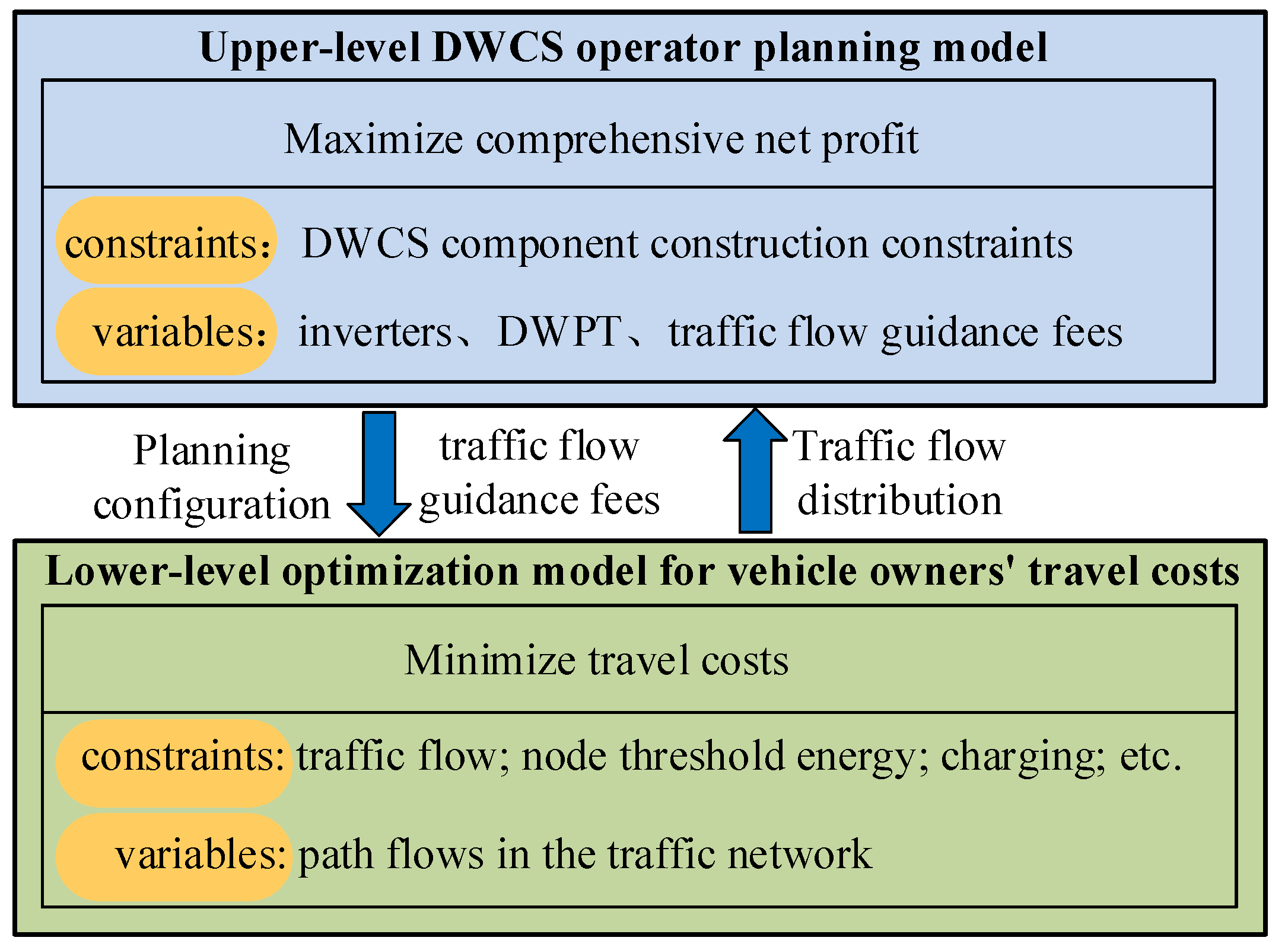
To address the shortcomings of existing DWCS bi-level optimization research, which overlooks EV owners’ travel choices and lacks the ability to actively regulate traffic congestion, this paper proposes a bi-level optimization model incorporating a traffic flow guidance mechanism. This model characterizes users’ travel choice behavior and reveals the dynamic interaction mechanism among DWCS planning, owners’ travel choices, and traffic flow distribution, thereby generating a more coordinated planning scheme. Within this framework, the upper-level operator jointly optimizes DWCS planning and pricing strategies. This allows for active steering and reshaping of traffic flow in the lower level. Meanwhile, EVs in the lower level make route choices by considering travel time costs, charging costs, and traffic flow guidance fees. This design marks a significant shift in system optimization. It moves from the traditional passive approach of “planning infrastructure based on fixed traffic flows” to an active co-optimization mode.
Therefore, to address these limitations in dynamic collaboration mechanisms and active guidance strategies, this study proposes a bi-level optimization model for transportation networks integrated with DWCS. The key contributions are outlined as follows:
First, this study proposes a dynamic collaborative coupling mechanism. This approach overcomes the limitation of treating traffic flow as a static input. It clarifies the triple interactive relationship among DWCS optimal planning, owners’ travel choices, and traffic flow distribution. Consequently, it provides a new logical framework for balancing operators’ revenue and owners’ travel costs.
Second, we develop a bi-level optimization model embedded with a traffic flow guidance mechanism. The upper-level maximizes operators’ annual net profit by optimizing DWCS planning and guidance fee parameters. Meanwhile, the lower-level minimizes owners’ comprehensive travel time costs based on the user equilibrium. This structure effectively alleviates peak-hour congestion and facility-demand mismatch.
Third, a quantitative analysis framework is established to evaluate the synergistic effects of key technical parameters. It reveals the interactive impact of EV battery capacity and unit energy consumption on DWCS planning costs and changes in traffic flow. These insights provide decision support for operators to dynamically adjust planning strategies according to technological evolution.
The remainder of the paper is organized as follows:
Section 2 elaborates on the bi-level optimization framework for the DWCS.
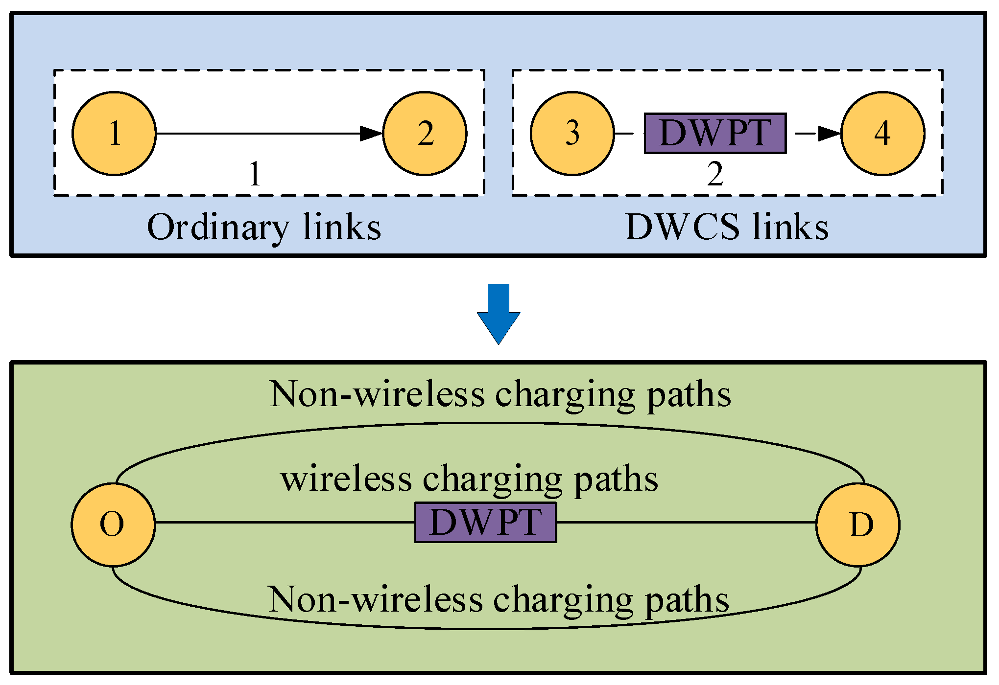
Section 3 presents the network modeling that incorporates the DWCS.
Section 4 details the lower-level travel model based on the user equilibrium principle.
Section 5 formulates the upper-level planning model, which aims to maximize the operator’s annual net profit.
Section 6 introduces the solution methodology for the bi-level model.
Section 7 validates the proposed model through case studies and conducts a sensitivity analysis of key technical parameters.
Section 8 summarizes the research conclusions and outlines directions for future work.
6. Solution Methodology for the Bi-Level Model
6.1. Reasons for Selection and Comparative Analysis of the Solution Algorithm
- (1)
Applicability Limitations of Traditional Bi-level Optimization Methods
The lower-level user equilibrium problem in this model exhibits several non-standard features. These characteristics make it difficult to effectively implement classical bi-level optimization methods. First, the lower-level user equilibrium problem has a large dimension and is highly nonlinearly coupled with the upper-level DWCS planning. This coupling invalidates traditional analytical methods, such as KKT conditions and gradient-based algorithms. Second, although the path generalized cost function is strictly convex, the non-monotonic property of charging power leads to a non-convex and multi-modal structure in the lower-level objective function. Consequently, convexity-dependent methods, such as sequential quadratic programming, struggle to converge stably. In addition, an implicit black-box mapping exists between the upper and lower levels. The upper-level traffic flow guidance fee affects flow distribution indirectly through path costs. However, this mapping is implicitly defined by the user equilibrium iteration. It is non-differentiable and difficult to approximate using surrogate models. These limitations hinder the application of sensitivity analysis and gradient backpropagation.
- (2)
Adaptive Advantages of the Heuristic-CPLEX Iterative Framework
To address these challenges, this study adopted an iterative solution strategy combining heuristic algorithms with CPLEX. The upper level involved a mixed-integer nonlinear programming problem with binary variables. CPLEX solved this exactly for DWCS facility location and capacity allocation, ensuring global optimality of the planning scheme. Conversely, the lower level handled the user equilibrium problem with nonlinear congestion via heuristic algorithms, ensuring quick convergence to the network flow equilibrium state. Through alternating iterations, the framework leveraged the robust search ability of heuristics and the computational efficiency of CPLEX. This effectively overcame difficulties such as the curse of dimensionality, non-convexity, multi-modality, and implicit mapping. Thus, it provided a stable and feasible approach for solving highly nonlinearly coupled bi-level programs.
6.2. Iterative Solution and Flow Chart
The model is solved using an iterative solution method [
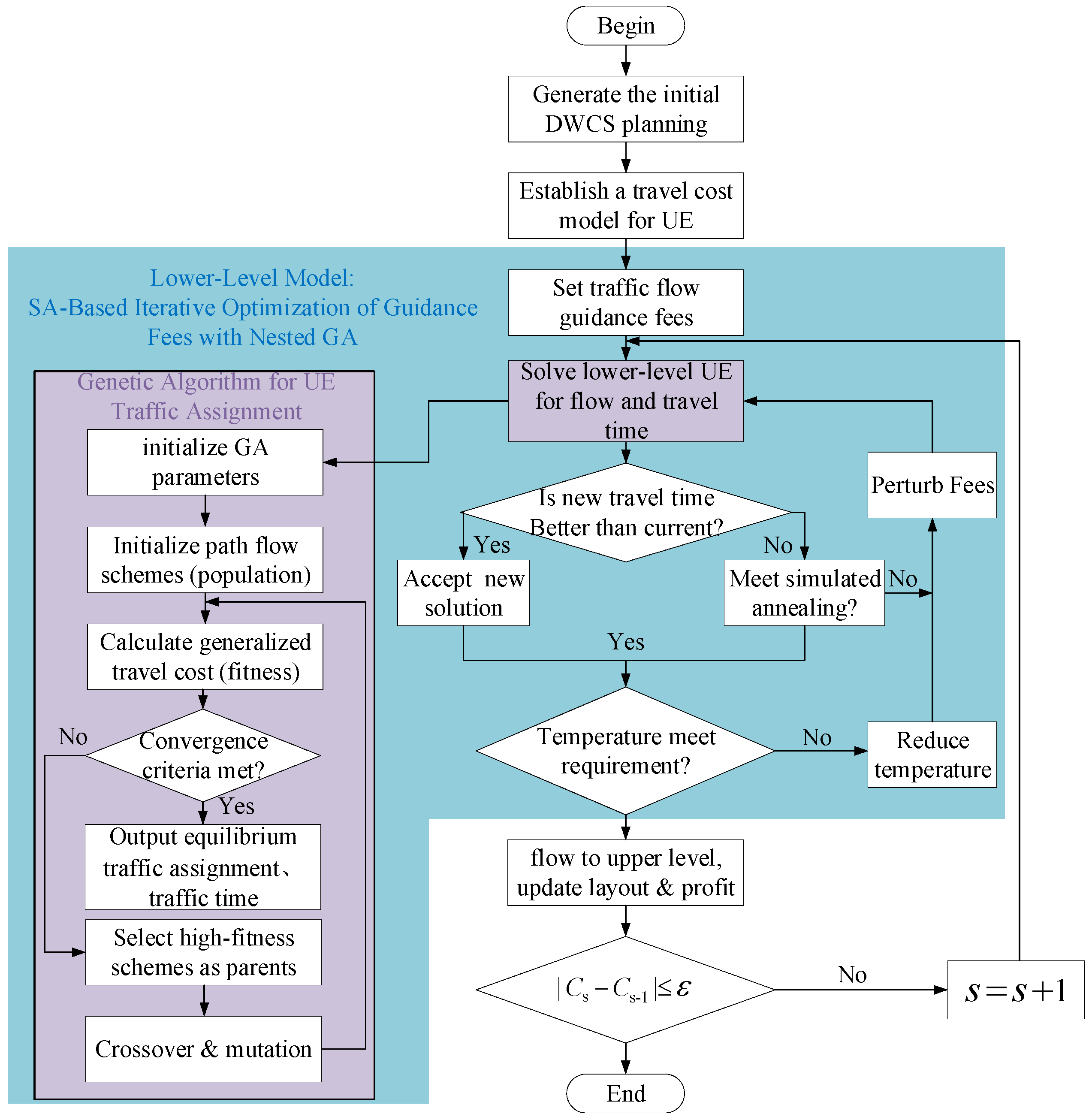
20]. In each iteration, the upper-level model first generates an initial DWCS planning scheme and a set of traffic flow guidance fees, which are then passed to the lower-level model. Upon receiving this information, the lower-level model solves for the resulting traffic flow distribution using a GA and obtains the corresponding total travel time as an initial solution. Subsequently, a joint iterative optimization based on SA-GA is implemented until the temperature requirement is met (i.e., the current temperature is lower than the preset termination temperature). At this point, the iterative optimization loop of the lower-level algorithm terminates, and the obtained annual travel flow is fed back to the upper-level model. The upper-level and lower-level models are solved alternately and iteratively until the upper-level model satisfies the convergence condition shown in Equation (35), at which point the process ends.
where
is the number of iterations for solving the bi-level model, and
is the convergence threshold. The overall solution process of the DWCS bi-level optimization model proposed in this study is shown in
Figure 3.
6.3. Feasibility-Preserving Mechanism for the Lower-Level User Equilibrium
To ensure that the lower-level user equilibrium solution always satisfies the physical and modeling constraints during the bi-level optimization process, a feasibility-preserving mechanism is incorporated into the algorithm design in this paper.
- (1)
Feasibility of Chromosome Encoding and Initialization
The GA encoded the variables to be solved into chromosomes. Each chromosome corresponded to a complete link flow distribution scheme, with each gene representing the flow assigned to the corresponding path. The number of paths defines the length of a single chromosome. The population size was set to 60, and the maximum number of iterations was 80. The offspring size was 80% of the parent population, with a mutation probability of 0.01. The number of genes selected for crossover and mutation was 3 and 4, respectively. The initial assignment was randomly generated. The flow of the last path was then adjusted to satisfy the flow conservation equation, yielding an initial solution that met flow conservation requirements.
During population initialization, a heuristic random generation method was adopted. For each O-D pair, the algorithm randomly selected a path from its feasible path set and assigned it a random flow value. Subsequently, normalization was performed to ensure the total flow for each O-D pair matched the demand. This procedure guaranteed that the initial population satisfied all flow conservation constraints.
- (2)
Feasibility of Crossover and Mutation
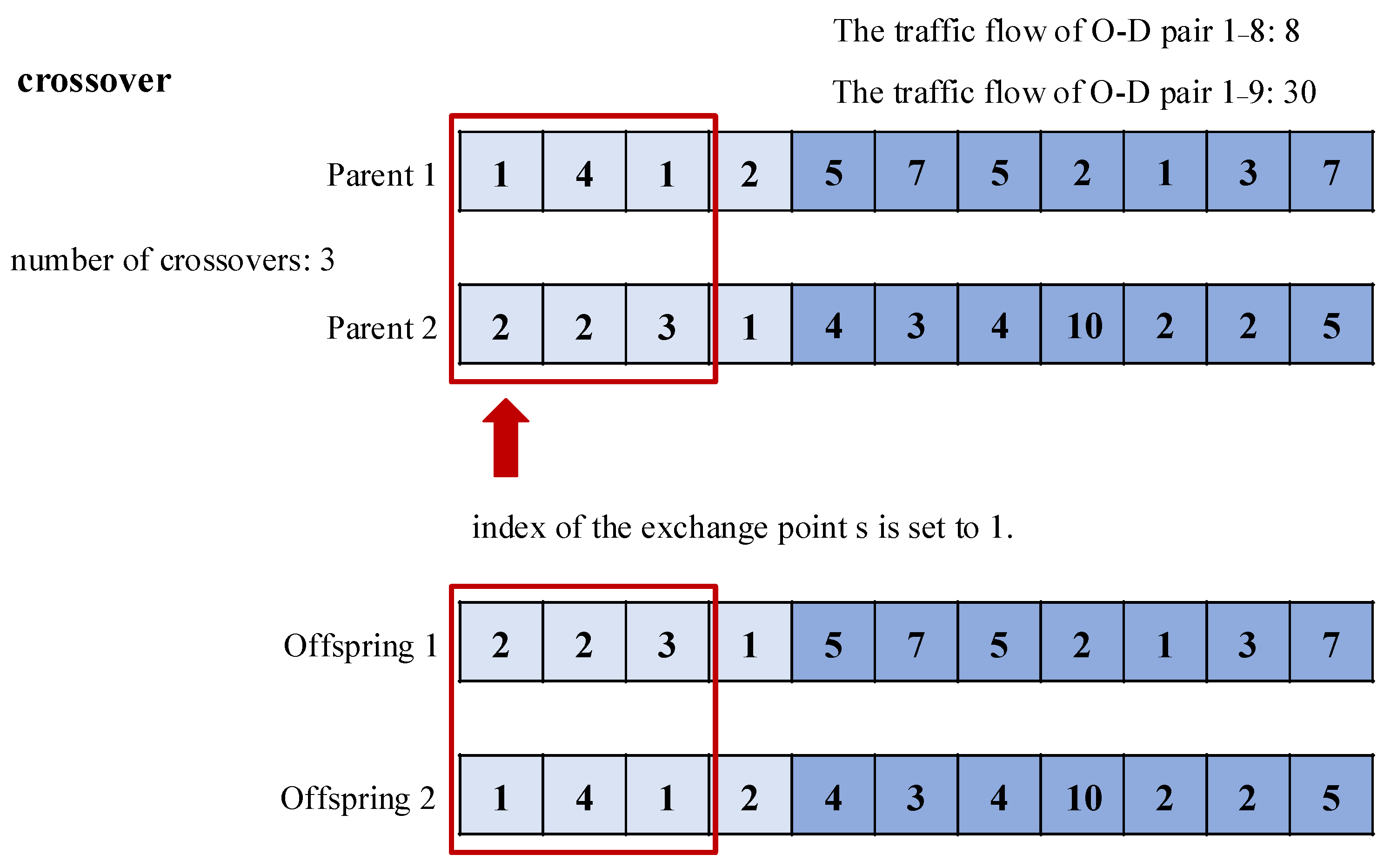
An improved multi-point crossover operator was adopted for the crossover operation. Chromosomes were encoded in segments based on the path flows of two O-D pairs (1–8 and 1–9), as shown in
Figure 4 (The data in the first four light blue boxes represent the number of vehicles on each of the four paths in O-D pair 1–8, and the data in the next seven dark blue boxes represent the number of vehicles on each of the seven paths in O-D pair 1–9). During crossover, three crossover points were randomly generated, and the path flows of the parent chromosomes at these points were exchanged sequentially (In the figure, taking the crossover points located at the first three gene loci as an example, the red arrows point to the boxes indicating where the exchange occurs between the two parent chromosomes. The exchanged genes are shown in the middle and lower boxes, based on which the offspring are generated.). The crossover operation was conducted within the same O-D pair to ensure that the exchanged flows still belonged to the feasible path set of that O-D pair. After the crossover, the flows of each O-D pair were normalized so that their sum strictly equaled the traffic demand in the corresponding period, thereby satisfying the flow conservation constraints. If negative values or constraint violations occurred after adjustment, the crossover was abandoned, and the parent individual was retained.
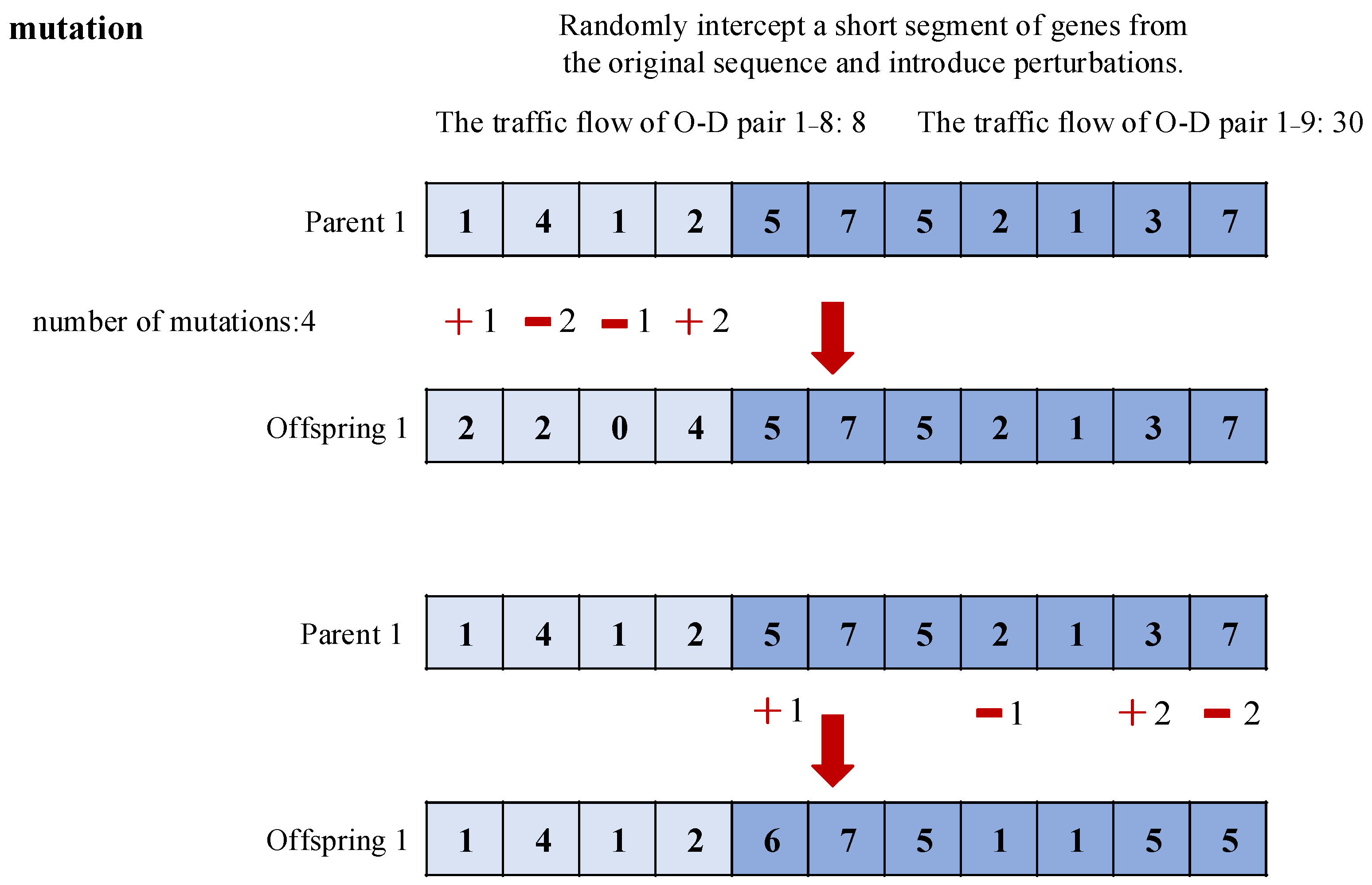
The mutation operation maintained flow conservation through intra-O-D flow shifting, as shown in
Figure 5. Two paths within the same O-D pair (1–8 or 1–9) were randomly selected. A portion of the flow (not exceeding a preset fluctuation value) was transferred from one path to the other, ensuring that both paths maintained non-negative flows and neither exceeded the total demand of the O-D pair (As shown in the figure, the flow from paths 2 and 3 in the parent O-D pair 1–8 is transferred to paths 1 and 4 to generate the offspring; the flow from paths 4 and 7 in the parent O-D pair 1–9 is transferred to paths 1 and 6 to generate the offspring). If the transfer violated flow constraints, the mutation was canceled.
- (3)
Feasibility of State-of-Charge Constraints
A SOC feasibility check was performed for each candidate path: the recursive SOC process of the vehicle from origin to destination was simulated in accordance with Equation (14). Only paths where the SOC remained above the minimum threshold at all nodes were retained, forming the feasible path set for each O-D pair.
- (4)
Feasibility of User Equilibrium Conditions
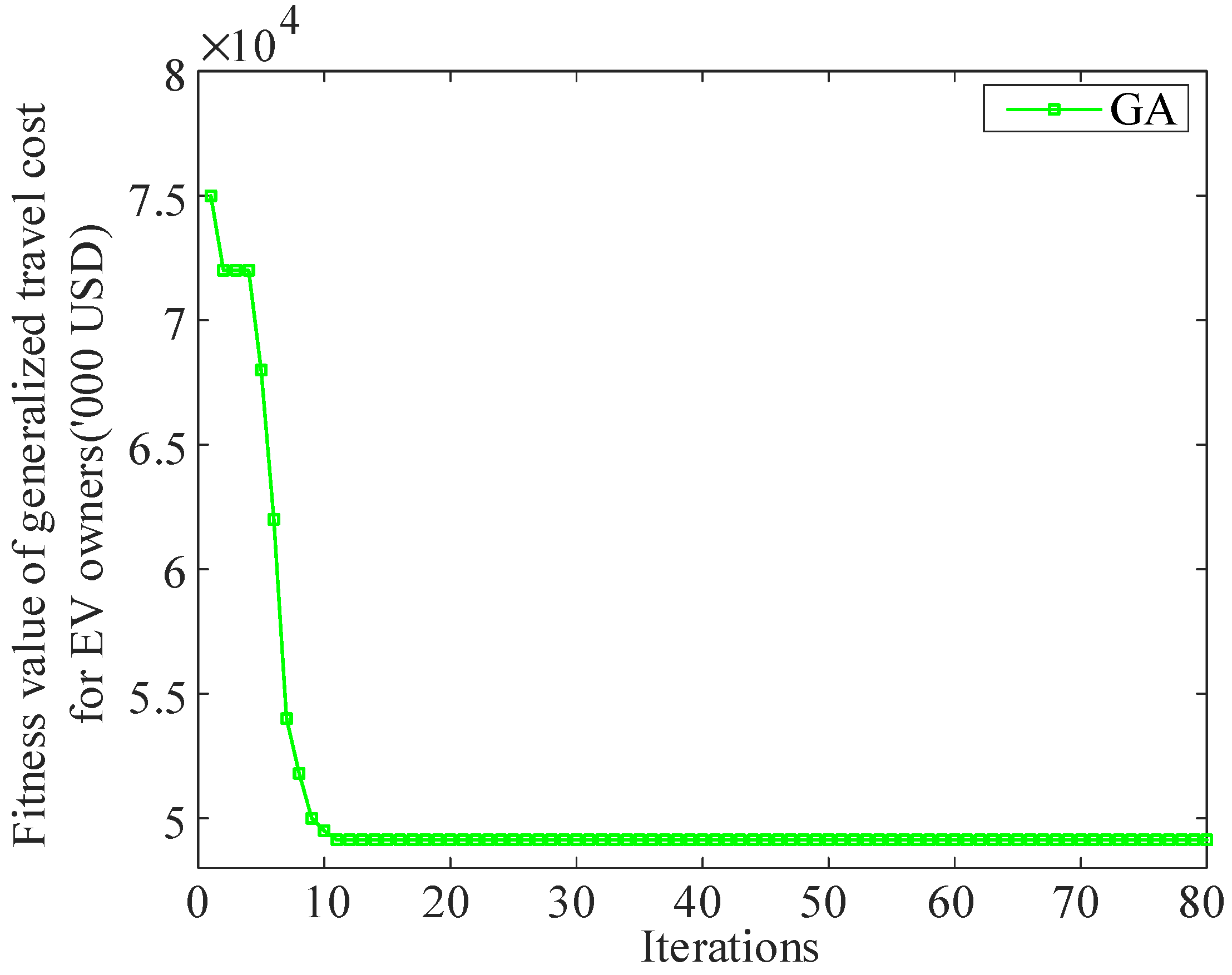
The lower-level model takes the minimization of the generalized travel cost of the transportation network as its objective function, which is directly used as the fitness function of the GA in this paper. Experiments show that the algorithm generally converges to a stable solution within approximately 11 iterations, and the solution always meets the feasibility requirements of UE under the protection of the aforementioned mechanisms.
6.4. Algorithm Flow
The collaborative simulation algorithm flow chart for the bi-level optimization problem is shown in Algorithm 1:
| Algorithm 1: Collaborative Simulation Algorithm for Bi-Level Optimization Problems in DWCS |
1. Algorithm Input
Transportation network parameters: , , , , , input via matrix, corresponding to Equations (1), (2) and (5)
DWCS parameters: , , , , , parameter input, corresponding to Equations (4) and (30)–(32)
Electricity price parameter: , , input via matrix, corresponding to Equations (6), (22) and (33)
Electricity quantity parameter input via matrix, corresponding to Equation (15)
Algorithm parameter: convergence threshold parameter input, corresponding to Equation (35)
2. Algorithm Steps
Step 1: Initialization
● Initialize facility planning scheme by matrix input, corresponding to Equation (3)
● Initialize the traffic flow guidance fee scheme input via matrix, corresponding to Equation (21)
Step 2: Main Iteration Loop
while not converged do
(1) Lower-level optimization (vehicle owner operation layer)
Input: current planning scheme
(1.1) SA initialization: set current temperature and current traffic flow guidance scheme
(1.2) Search loop (temperature > termination temperature)
(a) Generate new solution: apply random perturbation to traffic flow guidance fees to generate a new traffic flow guidance fee scheme
(b) Solve equilibrium with fixed Traffic guidance fees (call GA)
i. GA framework initialization: chromosome length (number of paths), population size (path scale), maximum number of iterations, offspring ratio, offspring population size, number of genes selected for crossover operation, mutation probability, number of genes selected for mutation
ii. Population initialization: generate the initial upper-level population (initial traffic flow allocation scheme), ensuring that the total traffic flow of each O-D pair equals the demand to satisfy: the flow conservation Constraints (9) and (10) satisfied by normalization, non-negative flow Constraint (11), and path feasibility Constraints (12) and (13)
iii. Fitness evaluation:
- Validate each traffic flow individual: traverse each node to calculate the electricity quantity conservation Constraints (14) and (15), electricity quantity threshold Constraint (16), and charging power Constraint (17)
- Traverse each node to calculate the charging power (4)
- Calculate the generalized travel costs (5–8)
- Calculate the generalized travel cost of the system as the fitness value (20)
- Select individuals with better fitness as parents
iv. Genetic operation: select, crossover and mutate according to fitness to generate a new generation of the population
v. Iteration and convergence: repeat evaluation and evolution until the GA terminates and converges to obtain the user equilibrium condition (18). Output the optimal traffic flow distribution and the corresponding minimum system travel time
(c) SA acceptance decision:
Time cost difference:
If , accept the new solution;
else, Accept with probability
(d) Update and cooling:
If the new solution is accepted, update it
After completing L searches at the current temperature, decrease the temperature
(1.3) Output lower-level results
(2) Upper-level optimization (planning layer):
Input: Traffic flow distribution
(2.1) Construct MIP model:
- Decision variables: binary variables DWPT, Inverter
- Objective function: calculate the upper-level objective function (22)
- Constraints: determine the node inverter planning using logical constraint rules (23–29)
(2.2) Solve: Call CPLEX to solve the MIP, and obtain:
● New DWPT planning
● Inverter planning
● Total profit of the operator
(3) Check convergence condition:
If then
The algorithm converges and exits the loop
Else pass the new facility planning scheme to the lower level and return to Step (1)
end if
end while
3. Output final results
When the main iteration loop terminates due to convergence, the optimal facility planning scheme is obtained. |
7. Case Study
In this section, to verify the performance of the proposed model, we conduct numerical simulation analysis based on the transportation network model adopted in references [
13,
17]. The network is shown in
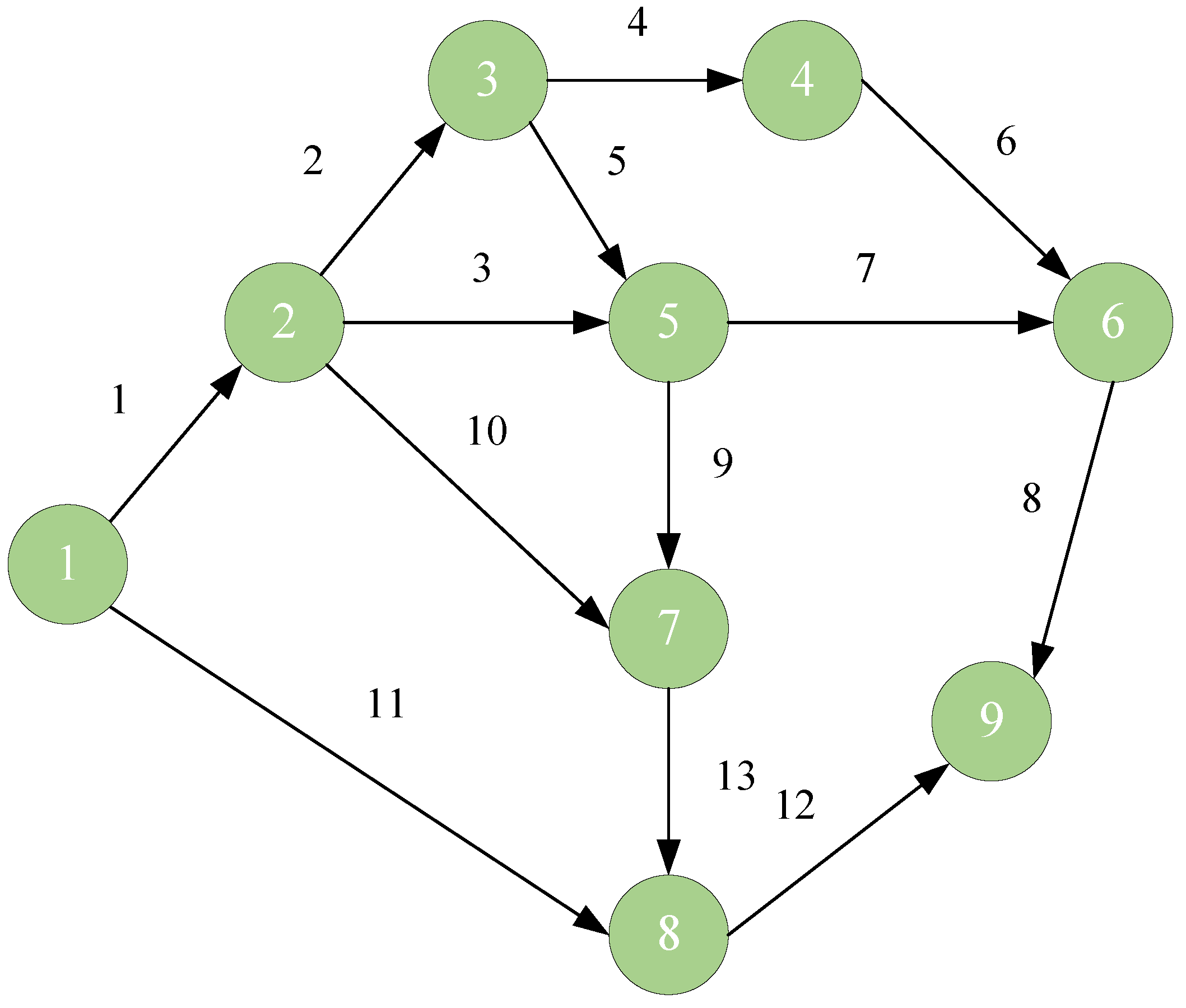
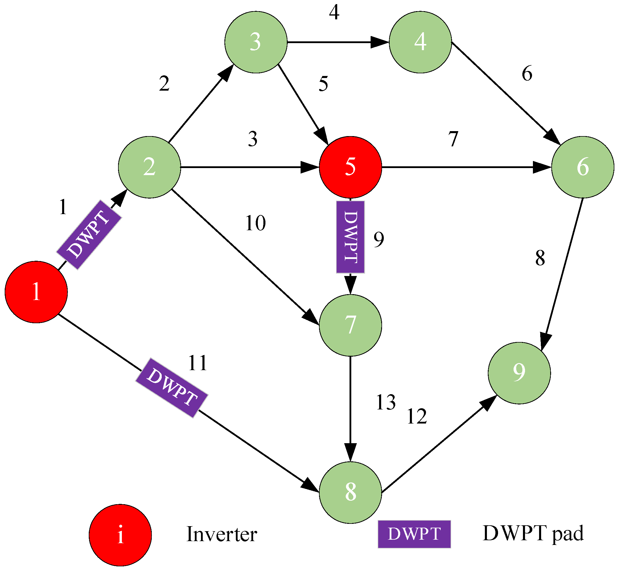
Figure 6, which contains 9 nodes and 13 links (The arrows in the figure indicate the direction of travel on each link, representing the permissible flow direction of traffic.). The data on link length, capacity, and free-flow travel time are shown in
Table 1. The O-D pairs of vehicles are nodes 1–8 and 1–9 in the network. The shortest path method is used to generate valid path sets for each O-D pair, as shown in
Table 2. The 24 h traffic demand of O-D pairs on a typical day is shown in
Table 3.
The charging power capacity per kilometer of DWCS is 65.79 MW [
21], the purchase cost of DWPT is 188.34 USD/m [
4], the purchase cost of an inverter is 14,127.75 USD/unit, and the annual maintenance cost per unit length of DWCS is 65.93 USD/m [
5].
According to statistics from the UK Department for Transport, the rated battery capacity of EVs is set to 50 kWh [
22]. Based on a study on the lifecycle aging behavior of lithium-ion batteries, the actual usable battery capacity degrades to below 90% of the rated battery capacity at the 400–cycle aging inflection point, entering the accelerated aging stage [
23]. Therefore, the actual usable battery capacity is set to 45 kWh. To control the battery depth of discharge, extend battery life, and ensure travel reachability, this study sets the minimum battery SOC threshold of the EV at 12 kWh. The battery energy consumption of the EV is 0.25 kWh/km, the maximum DWCS charging power is 60 kW [
16], and the charging efficiency is 0.9. The initial SOC of the EV at departure is uniformly distributed between 15 kWh and 45 kWh. This study refers to the time cost model proposed in reference [
16] and converts the monetary value of vehicles’ travel time via exchange rate and unit conversion, yielding 11.26 USD/h. The time-of-use electricity price is shown in
Table 4. The parameter values are shown in
Table 5. This study uses the MATLAB 2021b environment and combines the CPLEX solver for an iterative solution to obtain the optimization scheme.
7.1. Simulation Comparison
7.1.1. Two-Level Optimization Scenario Setting for DWCS
Based on the user equilibrium principle, in addition to considering the scenario of full coverage of DWCS, this study also constructs three simulation scenarios and conducts a comparative analysis:
Scenario 1: Considering the optimal travel plan for EV owners, a bi-level optimization scheme for DWCS is proposed.
Scenario 2: By introducing traffic flow guidance fees to regulate traffic flow and based on reducing travel time, considering the optimal travel plan for EV owners, a bi-level optimization scheme for DWCS is proposed.
Scenario 3: Adopting the same DWCS optimization scheme as Scenario 2, considering the optimal travel plan for EV owners with fixed planning, without introducing traffic flow guidance fees.
7.1.2. Planning Results of DWCS
The planning of DWCS in full coverage, Scenario 1, Scenario 2 and Scenario 3 are as follows:
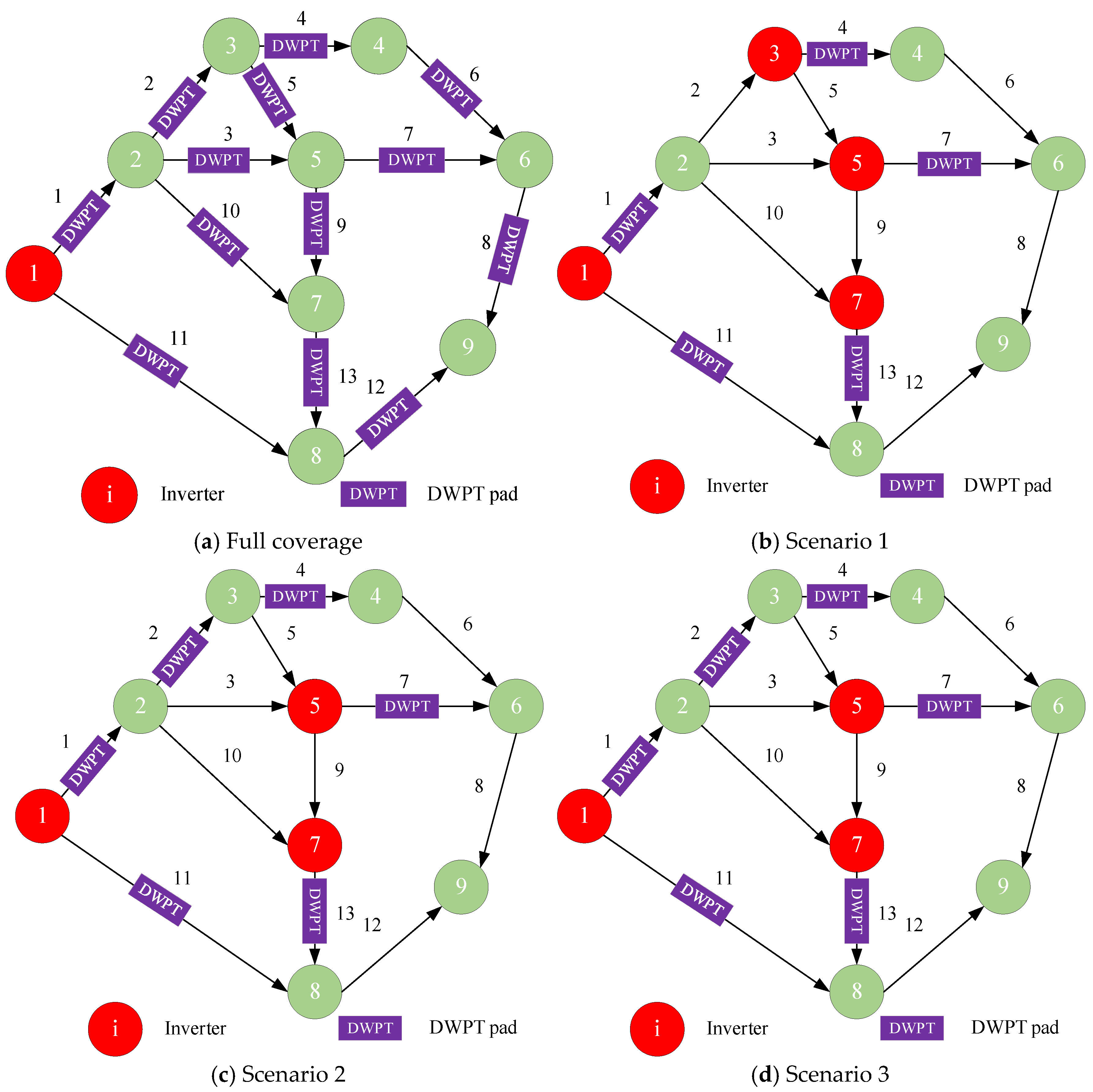
Figure 7 presents the planning results of four DWCSs (The numbers 1–13 in the figure represent the link numbers. The purple boxes indicate links equipped with DWPT, the red nodes represent nodes equipped with inverters, and the green nodes represent ordinary nodes). The scheme shown in
Figure 7a is equipped with a total of one inverter, located at node 1; a total of 13 DWPTs are deployed, on links 1 to 13, with the total deployed length accounting for 100% of the total length of the road network. The scheme shown in
Figure 7b is equipped with a total of four inverters, located at nodes 1, 3, 5, and 7 respectively; a total of five DWPTs are deployed, on links 1, 4, 7, 11, and 13 respectively, with the total deployed length accounting for 44.05% of the total length of the road network. The scheme shown in
Figure 7c is equipped with three inverters, located at nodes 1, 5, and 7; a total of six DWPTs are deployed, on links 1, 2, 4, 7, 11, and 13 respectively, accounting for 52.38% of the total length of the road network, which is the same as Scenario 3 (
Figure 7d).
7.1.3. Comparative Analysis of Optimization Results Between Scenario 1 and the Full-Coverage Scenario
As shown in
Table 6, compared with the annual loss of −6163.06 thousand USD in the full-coverage scenario, the annual net loss of the operator in Scenario 1 is reduced to −775.35 thousand USD, with a loss reduction of 5387.71 thousand USD, achieving a narrowing of losses; the owners’ travel cost is reduced by 18,036.38 thousand USD.
This result is mainly attributed to the following optimization mechanisms: On the DWCS operator side, by optimizing facility planning while ensuring each vehicle can reach its destination smoothly with sufficient power, resource redundancy caused by the full-coverage mode was effectively avoided. This reduced the DWPT installation cost by 55.63% and the DWCS maintenance cost by 55.95%. On the owners’ side, Scenario 1 directly reduced owners’ charging expenses by 18,616.62 thousand USD by eliminating invalid charging in the full-coverage scenario, thereby significantly lowering their overall travel costs.
Compared with the full-coverage scenario, Scenario 1 optimized planning on the upper-level DWCS planning side, but this scheme did not significantly improve travel time costs for owners. Meanwhile, although losses were reduced, the operator remained in a state of loss. In fact, the travel time of vehicles in the transportation network with DWCS directly affects charging costs, overall travel costs, and road congestion levels, and indirectly changes traffic flow distribution. In turn, traffic flow distribution affects the planning profit of DWCS operators and the travel costs of owners. For this reason, we propose Scenario 2 to optimize travel time through a traffic flow guidance fee mechanism and analyze it by comparing Scenarios 1 and 3.
7.1.4. Comparative Analysis of Optimization Results Between Scenario 2 and Scenarios 1 and 3
As shown in
Table 6, compared with Scenario 1, although the total construction and maintenance cost of Scenario 2 increases by 1765.76 thousand USD, the comprehensive net profit increases significantly by 2742.13 thousand USD. At the same time, owners’ charging expenses increase by 1984.15 thousand USD, while the travel time cost decreases substantially by 6740.58 thousand USD.
This is because Scenario 1 optimizes the DWCS planning to match traffic demand based on the traffic flow distribution formed by owners’ path choices, avoiding resource waste. However, this approach does not alter the underlying traffic congestion pattern, leading to relatively high time costs for owners. In contrast, Scenario 2 regulates traffic flow through traffic flow guidance fees, alleviates traffic congestion, and significantly reduces owners’ time costs. Although Scenario 2 involves higher construction and maintenance expenditures due to the installation of additional DWCS facilities, the regulatory effect of the guidance fees indirectly stimulates a significant increase in charging volume. As a result, it achieves a net gain in charging revenue of 1883.52 thousand USD. Combined with the traffic flow guidance fee revenue of 2634.43 thousand USD, Scenario 2 achieves a net profit growth of 2742.13 thousand USD. Although owners bear an additional charging expense of 2634.43 thousand USD, they gain a time cost saving of 6740.58 thousand USD, resulting in a net welfare increase of 2122 thousand USD. Furthermore, to isolate the direct contribution of the traffic flow guidance fee mechanism, this study introduces Scenario 3 as a control scheme. In this scenario, the guidance fee mechanism is removed, while the facility planning solution from Scenario 2 is held unchanged. The comparative analysis yields the following results:
Compared with Scenario 3, the annual comprehensive net profit of the operator under Scenario 2 increases by 3717.68 thousand USD, and the owners’ travel cost decreases by 2433.48 thousand USD. Among these, the owners’ travel time cost decreases by 6421.18 thousand USD, which becomes the main factor driving the reduction in owners’ travel cost.
Therefore, this study compares the estimated total travel time required to fulfill all owners’ travel demands under Scenarios 2 and 3 across different time intervals on a typical day, as shown in
Figure 8. From the perspective of daily total travel time, Scenario 2 achieves a 48.89% reduction compared to Scenario 3, indicating a substantial optimization in travel efficiency. Examining specific time periods, during the low-traffic intervals from 1:00 to 6:00 and 20:00 to 24:00, the difference in travel time between the two scenarios is minimal, largely due to naturally smooth traffic conditions. In contrast, during the peak hours from 7:00 to 19:00, the traffic flow guidance fee mechanism significantly mitigates the additional travel time typically caused by congestion.
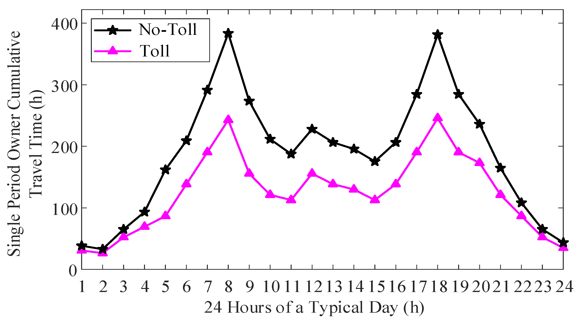
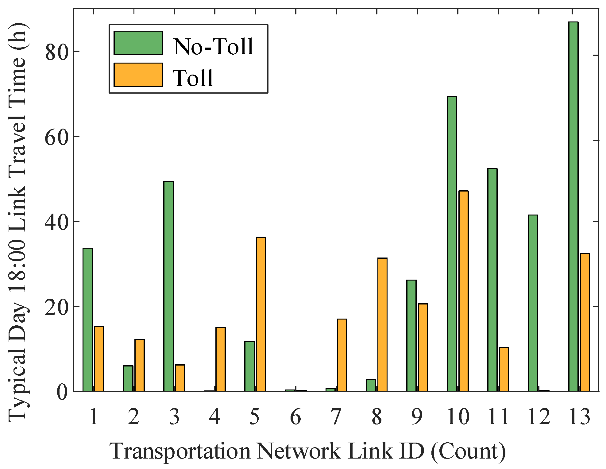
To further examine the regulatory effect of the traffic flow guidance mechanism during peak periods, this study selects the 18:00 peak hour on a typical day for analysis. It compares the travel time distribution characteristics of each link in the road network under two scenarios, as shown in
Figure 9. The results indicate that compared with Scenario 3, the total travel time in Scenario 2 decreases from 381.49 h to 245.82 h, representing a reduction of 35.56%. Moreover, the standard deviation of travel time across links in Scenario 2 is 50.76% lower than that in Scenario 3, suggesting a more balanced spatiotemporal distribution of traffic flow. These findings demonstrate that the traffic flow guidance mechanism can effectively guide the rational allocation of traffic flow, reduce excessive congestion duration on certain links, and promote balanced vehicle distribution across the road network, thereby significantly alleviating peak-period congestion and reducing owners’ travel time costs. Based on the annualized calculation of average daily travel time, owners’ travel time costs are substantially reduced, while the operators’ annual comprehensive net profit is significantly increased.
7.2. Algorithm Performance Analysis
7.2.1. Guarantee of Repeatability and Robustness
To ensure the repeatability and robustness of the research results, the following measures are adopted in this paper. First, regarding repeatability, all numerical experiments are performed under a unified computing environment (MATLAB R2021b for programming, IBM ILOG CPLEX Optimization Studio 12.10 from IBM Corp., Armonk, NY, USA as the solver). All parameter values of the model, constraints, and algorithm initialization methods are disclosed in the paper. The core hyperparameters of the adopted heuristic algorithm and the CPLEX iterative solution are provided in
Section 7.2.4.
Secondly, in terms of robustness, we conducted a parametric sensitivity analysis. As shown in the sensitivity verification table in
Section 7.2.4, the algorithm’s performance is insensitive to variations in key parameters such as crossover rate and mutation rate, and the quality of the obtained solutions remains stable when these parameters are adjusted within reasonable ranges. Furthermore, the stability of the algorithm was verified through multiple independent runs, with average performance metrics reported in
Section 7.2.2 (2). The convergence analysis (
Figure 10) further demonstrates that the algorithm can efficiently converge to a stable solution within a limited number of iterations.
7.2.2. Convergence Analysis of the Lower-Level Algorithm
- (1)
Numerical Convergence Verification
Figure 10 shows the convergence curve of the generalized travel cost solved by the lower-level GA after the upper-level SA perturbs the traffic flow guidance fee at the 60th temperature decrease (the global convergence optimal stage). The maximum number of iterations is set to 80, and the GA converges to the lower-level optimal solution under the near-optimal traffic flow guidance fee after approximately 11 iterations.
- (2)
Algorithm running time
The average time for the GA to converge to the lower-level optimal solution after about 11 iterations for the input traffic flow guidance fee is 2.3 s; the average total time for the SA to complete one perturbation of the traffic flow guidance fee and synchronously finish the whole lower-level GA solution is 2.4 s; when the SA achieves global convergence after 60 iterations with a chain length of 18 for each temperature decrease, the overall average running time of the lower-level algorithm is about 2592 s. With an upper-level convergence threshold of 1 × 10⁻³ and an average of 8 iterations, the total time of the bi-level programming is about 5.76 h.
7.2.3. Quantitative Analysis of Computational Complexity
Under the test scenario with 9 nodes, 13 links, and 2 O-D pairs, the time complexity of each module is analyzed as follows:
(1) SA component: With an initial temperature of 120, a cooling coefficient of 0.9, and termination temperature of 0.22, the number of temperature decay steps k ≈ 60, and 18 iterations within a single temperature step, the total operation complexity of SA is O (k × 18) = O (1080).
(2) GA component: With a population size of 60 and 80 iterations, a single GA run requires fitness evaluation for 60 individuals (including BPR function and SOC constraint verification), yielding a complexity of O (60 × 80) = O (4800). The total number of GA calls within a single bi-level iteration is 60 × 10 = 600, corresponding to a complexity of O (1080 × 4800) = O (5.18 × 10⁶).
(3) Bi-level iteration component: With an upper-level convergence threshold of 1 × 10⁻³, the average number of iterations is 8, and the total complexity of the overall algorithm is O (8 × 5.18 × 106) = O (4.14 × 10⁷).
7.2.4. Parameter Sensitivity Verification
The parameter sensitivity verification table is shown below. As can be seen from
Table 7, the number of iterations and initial temperature are the core sensitive parameters of the algorithm, while the others are secondary sensitive parameters:
7.3. Sensitivity Analysis
In the bi-level model, battery capacity and unit energy consumption determine the charging demand, which in turn affects the planning and capacity determination of upper-level facilities. Meanwhile, different traffic flows alter travel time and the distribution of charging demand and also exert a significant impact on the effectiveness of DWCS planning. For this reason, this section conducts a sensitivity analysis to quantify the impact of changes in the above factors on the optimization results, providing an adjustable planning basis for DWCS operators.
7.3.1. The Impact of Battery Capacity Changes on DWCS and Operational Benefits
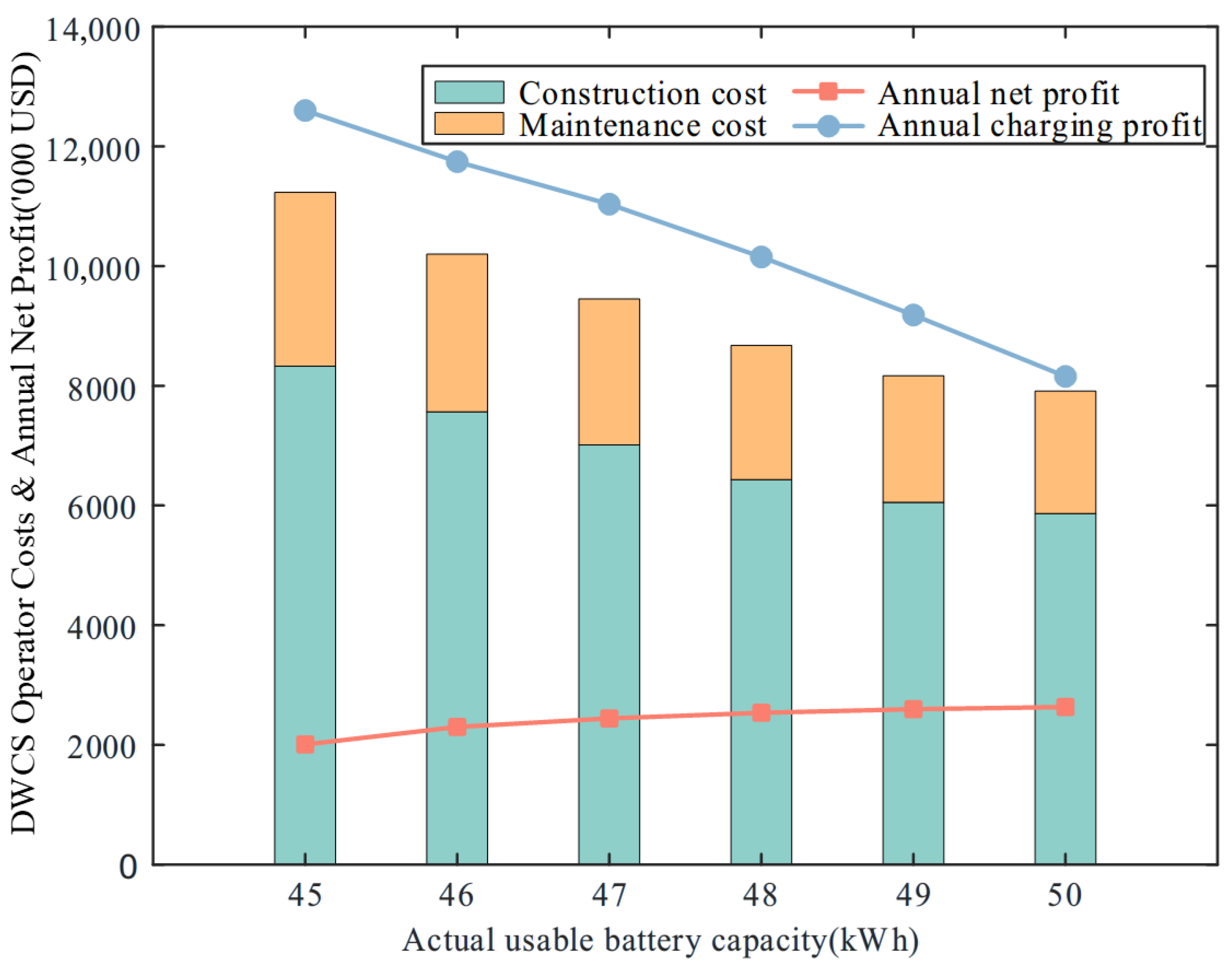
As the battery capacity increases from 45 kWh to 50 kWh (with other parameters unchanged),
Figure 11 shows the planning under the 50 kWh capacity, where the number and locations of inverters and DWPT have changed significantly. In
Figure 12, compared with 45 kWh, the construction cost and maintenance cost of the DWCS operator under the 50 kWh capacity have decreased by 2462.55 thousand USD and 857.09 thousand USD respectively, and the annual net profit has increased by 624.45 thousand USD.
With each 1 kWh increase in battery capacity, the mean state of charge rises from 30 kWh to 30.5 kWh, thereby shifting the distribution of charging thresholds for marginal vehicles. Taking O-D pair 1–8 as an example, the charging threshold for its shortest path (16 km) is 16 kWh—calculated as the minimum energy threshold (12 kWh) plus the route length multiplied by the energy consumption rate (0.25 kWh/km). Vehicles with initial energy in the [15, 16) kWh interval, therefore, require mid-journey charging. Each 1 kWh capacity increment reduces the expected number of such vehicles by approximately 3.23%; when capacity increases to 50 kWh (raising the mean to 32.5 kWh), the cumulative reduction reaches about 14.29%. Similarly, for O-D pair 1–9, the expected number of vehicles in the [15, 18) kWh interval declines by the same proportion. The reduction in marginal vehicles directly lowers charging demand density on certain road segments. This adjustment is propagated from the lower-level traffic assignment to the upper-level planning layer through the bi-level framework, ultimately triggering a reconfiguration of the charging network planning.
Further analysis reveals that the impact of capacity expansion on operator profitability is nonlinear. As capacity increases incrementally from 45 kWh to 50 kWh, the annual profit growth rates decline sequentially: 14.5%, 6.2%, 3.79%, 2.43%, and 1.4%. This diminishing trend arises from two counteracting effects: on one hand, higher capacity reduces the need for charging infrastructure, lowering planning costs; on the other hand, reduced charging demand along routes decreases revenue from charging services. At lower capacity levels, cost savings dominate; however, as capacity continues to rise, marginal cost savings diminish while charging revenue keeps falling in line with demand. The interplay of these two forces leads to a gradual slowdown in profit growth.
It should be noted that while increasing battery capacity can reduce dependence on DWCS, the manufacturing cost of large-capacity batteries remains relatively high, potentially compromising vehicle economics. Therefore, future research must balance the construction and maintenance costs of charging facilities against vehicle costs to achieve overall benefit optimization.
7.3.2. The Impact of Energy Consumption and Battery Capacity on the Construction and Maintenance Cost
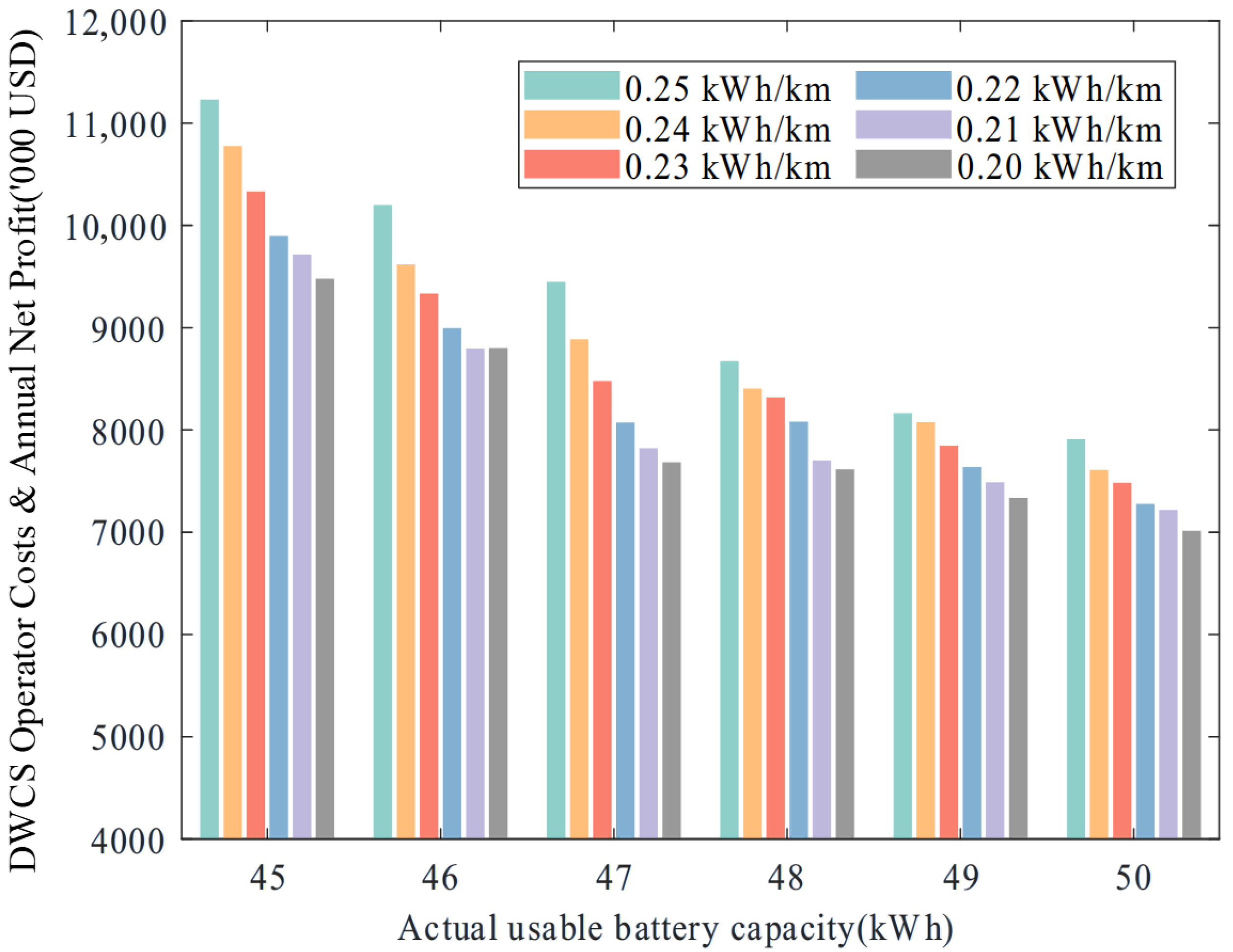
Figure 13 shows the significant impact of energy consumption and battery capacity on the total construction and maintenance costs of DWCS. Taking a battery capacity of 45 kWh as an example, as EV energy consumption decreases from 0.25 kWh/km to 0.20 kWh/km, charging demand declines accordingly. This reduced reliance on DWCS leads to a corresponding drop in total construction and maintenance costs.
When the battery capacity is 45 kWh, and the energy consumption rate is 0.20 kWh/km, the total construction and maintenance cost of the DWCS is substantially lower than in the scenario with a 44 kWh battery and a 0.25 kWh/km consumption rate. This finding suggests that, to maintain a given driving range, higher energy consumption necessitates a larger battery capacity. Energy consumption and battery capacity are closely interrelated, and this relationship directly influences the overall construction and maintenance costs.
7.3.3. Effectiveness of Traffic Flow Guidance Mechanism Under Varying Traffic Flows
To evaluate the planning effectiveness and control capability of introducing a traffic flow guidance mechanism under varying traffic demand conditions, this paper, based on the baseline flow distribution shown in
Table 3, further establishes two scenarios: 80% of the baseline flow (low flow) and 120% of the baseline flow (high flow). While keeping the DWCS planning scheme consistent with the corresponding traffic flow scenario, a horizontal comparison is conducted between two modes: “with traffic guidance mechanism” and “without traffic guidance mechanism.”
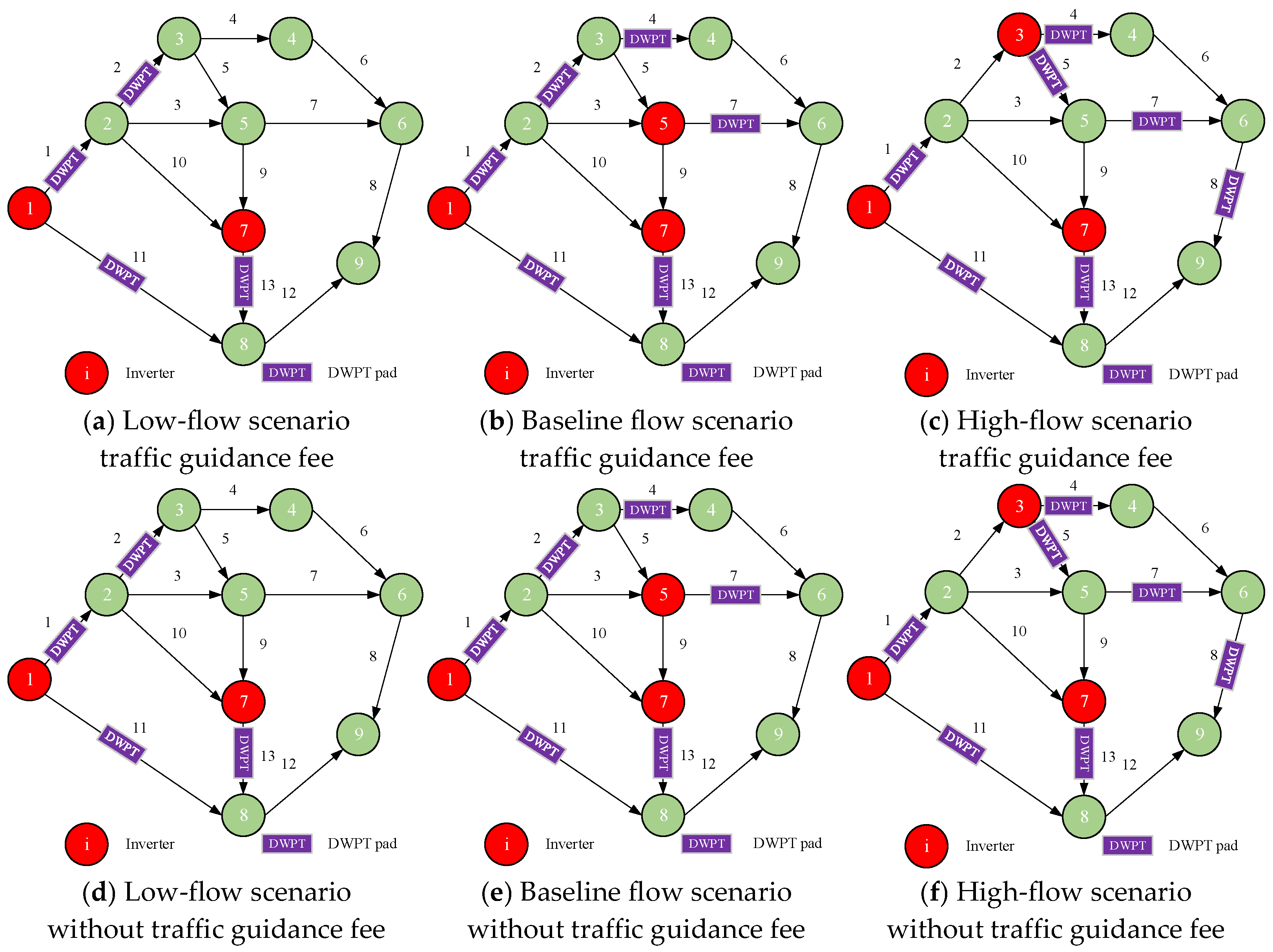
Figure 14 presents the planning results for the six comparative scenarios. In the low-flow scenarios shown in
Figure 14a,d, the road network is equipped with a total of two inverters, located at nodes 1 and 7 respectively; a total of four DWPTs are deployed, on links 1, 2, 11, and 13 respectively, with the total deployed length accounting for 47.61% of the total length of the road network. In the baseline flow scenarios shown in
Figure 14b,e, the road network is equipped with a total of three inverters, located at nodes 1, 5, and 7 respectively; a total of six DWPTs are deployed, on links 1, 2, 4, 7, 11, and 13 respectively, with the total deployed length accounting for 52.38% of the total length of the road network. In the scenarios shown in
Figure 14c,f, the road network is equipped with a total of three inverters, located at nodes 1, 3, and 7 respectively; a total of seven DWPTs are deployed, on links 1, 4, 5, 7, 8, 11, and 13 respectively, with the total deployed length accounting for 55.95% of the total length of the road network. This indicates that as traffic flow increases, the planning scale of DWCS (number of inverters, number of DWPTs, and total length) expands accordingly to meet higher charging demand.
As shown in
Table 8, after the introduction of the traffic flow guidance mechanism, the user travel time costs under the low, baseline, and high flow scenarios decreased by 29.7%, 32.2%, and 43.4%, respectively. This trend indicates that the regulatory capability of the traffic guidance mechanism may strengthen with increasing traffic flow, with its effect on alleviating congestion and saving travel time being relatively more prominent under the high-flow scenario.
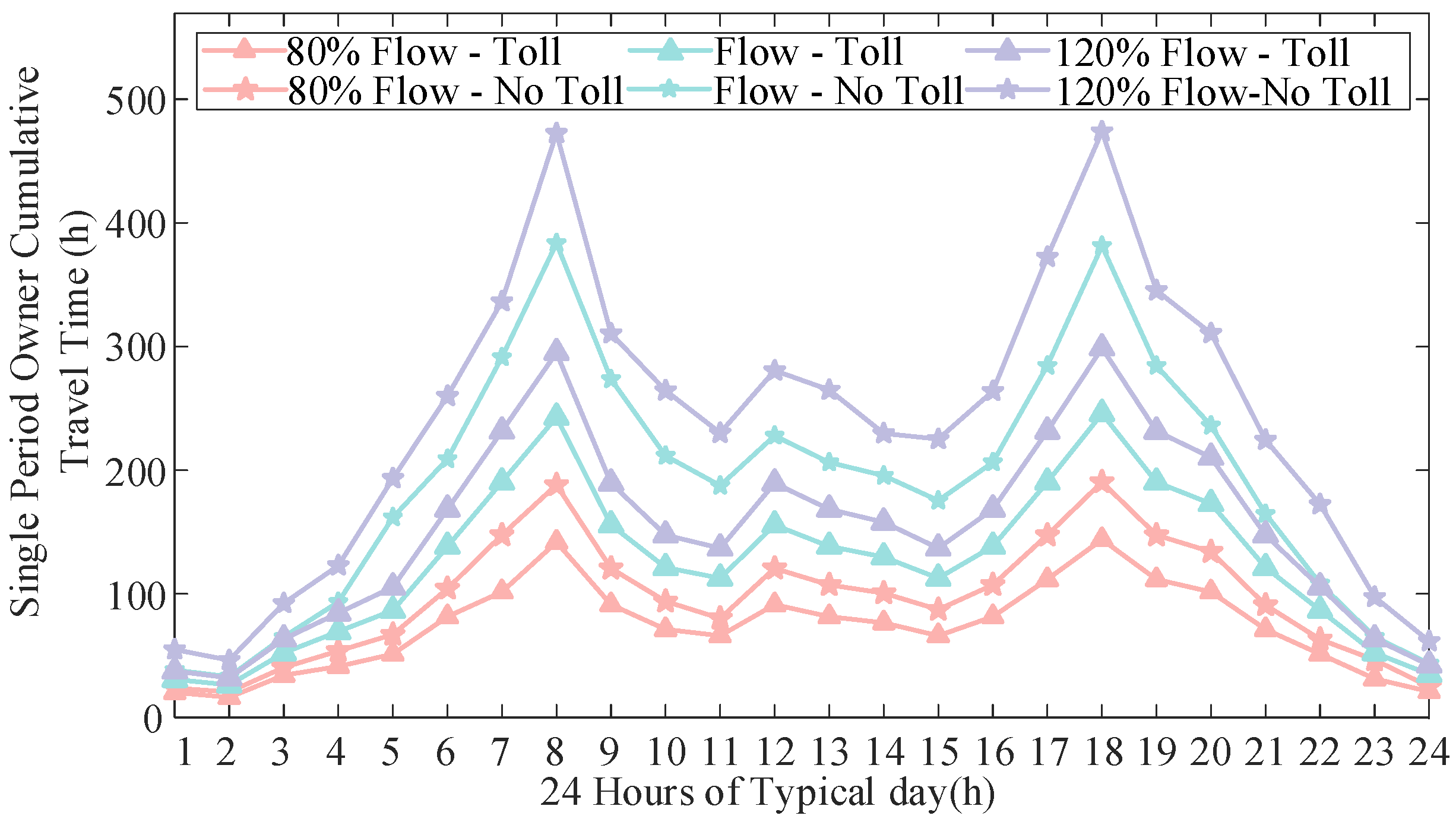
Based on this, combined with the comparison results of the 24 h cumulative travel time curves for a typical day under the six scenarios (
Figure 15), it can be observed that in the 80% low-flow scenario, the curves corresponding to with and without traffic guidance fee are relatively close overall, with relatively small differences in travel time across different periods. Under low-flow conditions, the traffic guidance mechanism has a relatively limited effect on travel choices. As the flow increases to the baseline level, the two curves show a certain degree of separation during the morning and evening peak hours (6:00–10:00, 15:00–20:00), with the cumulative travel time in the scenario without a traffic guidance fee increasing. The impact of the presence or absence of the traffic guidance fee on travel time begins to gradually emerge. In the 120% high-flow scenario, the degree of separation between the curves further widens, and the differences in travel time during the morning and evening peak hours become more pronounced. This reflects that under high-flow conditions, the absence of a traffic guidance mechanism may exacerbate congestion, while the effectiveness of the traffic guidance mechanism in reducing travel time is better demonstrated in this scenario.
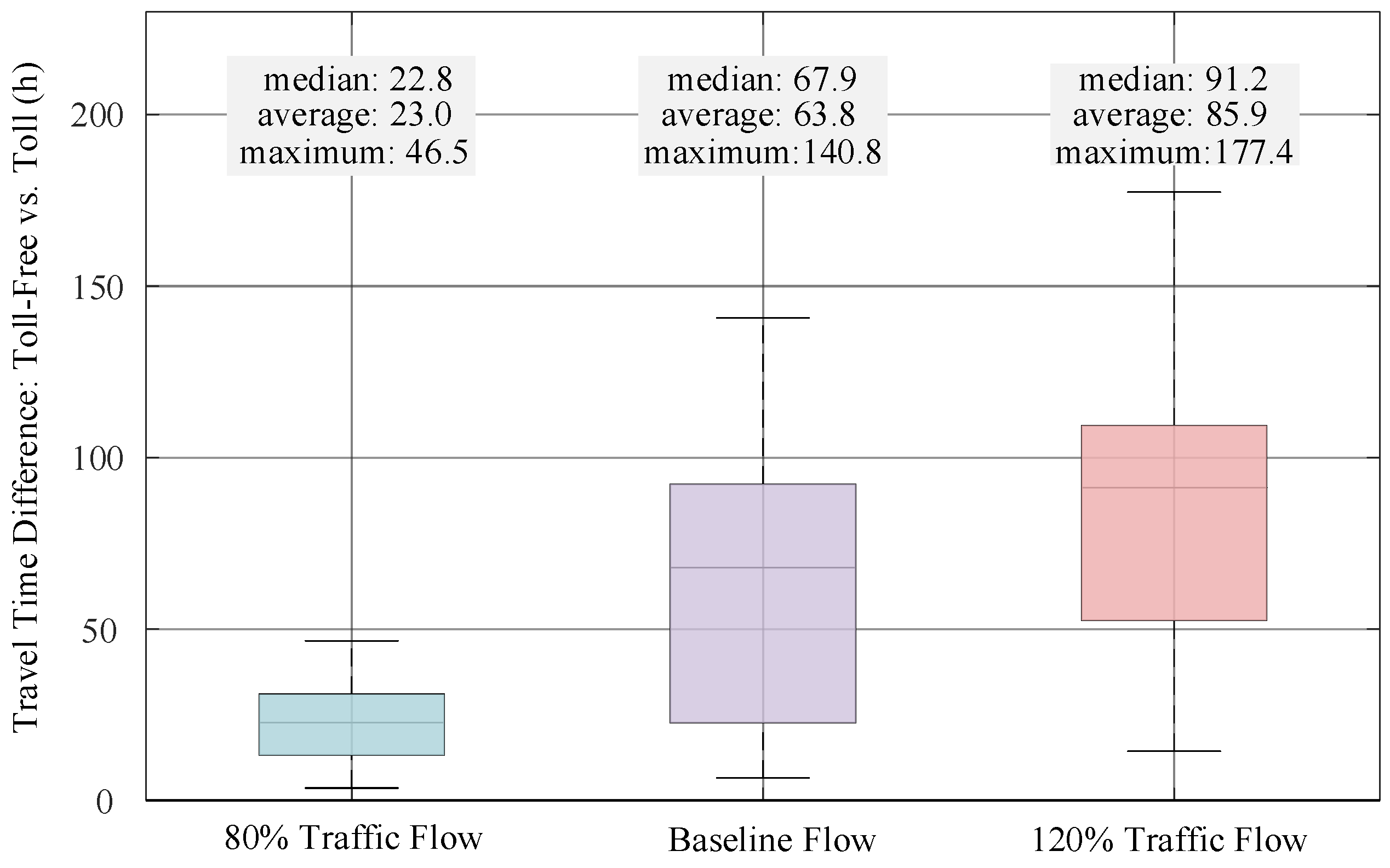
To further quantify the differences caused by the presence or absence of traffic guidance fees and variations in traffic flow from a statistical perspective, we analyze the travel time distributions under different flow scenarios using box plots (
Figure 16). In the 80% low-flow scenario, the box plot is relatively compact, with a median of approximately 22.8 h, and the overall distribution is close to the zero line. This indicates that the traffic system still maintains a certain redundant capacity under low-flow conditions. The influence of traffic guidance fees on travel choices is relatively limited, resulting in a mild overall impact on the total travel time.
When the traffic flow increases to the baseline level, the height of the box increases noticeably, with the median rising to approximately 67.9 h and the upper whisker increasing sharply to about 140.8 h. This demonstrates that under the baseline flow, the traffic system gradually approaches saturation. The absence of price signals from traffic guidance fees may exacerbate congestion in certain periods, thereby significantly enhancing the impact of traffic guidance fees on travel time.
In the 120% high-flow scenario, both the box height and whisker range are relatively large, with the median rising to approximately 91.2 h and the maximum individual difference reaching about 177.4 h. The overall distribution of the boxplot is clearly far from the zero line. This indicates to some extent that the traffic system tends to become saturated under high flow. The absence of traffic guidance fees may lead to a significant increase in travel time, and the role of traffic guidance fees in alleviating congestion and saving travel time is more fully demonstrated in this scenario.
Table 8 also demonstrates the impact of the traffic flow guidance mechanism on system economic efficiency under different traffic flow scenarios. Under low traffic flow, the operator’s loss narrows from 3230.63 thousand USD to 1496.72 thousand USD after introducing tolls. Under the baseline traffic flow scenario, the system turns into a profit, with a net profit of 1966.78 thousand USD. Under high traffic flow, the operator’s net profit surges from 578.93 thousand USD to 5437.87 thousand USD. As traffic volume increases, the role of tolls in improving operator revenue becomes increasingly prominent. In addition, toll revenue also rises significantly with increasing traffic volume, from 1053.77 thousand USD to 3834.39 thousand USD, reflecting that the regulatory intensity of tolls strengthens with the growth of traffic flow.
7.4. Comprehensive Discussion
- (1)
Discussion on More Complex Topologies
At the model structure level, the upper-level planning model aims to maximize the annual net profit of the DWCS operator. Its decision variables include the planning locations of DWPT and inverters, as well as the traffic flow guidance fee, all of which are defined on links and nodes. When the road network scale expands, only the number of decision variables corresponding to links and nodes needs to be increased, while the model structure itself remains unchanged.
At the computational level, to address the curse of dimensionality in large-scale road networks, the framework proposed in this paper can be adapted through parallel computing and distributed optimization architectures. The lower-level user equilibrium model involves flow assignment for multiple O-D pairs. Since the calculations for different O-D pairs are relatively independent, the problem can be decomposed into several subtasks for parallel solution and then converge iteratively via a boundary coordination mechanism. In the upper-level planning model, DWPT planning decisions and traffic flow guidance fees on different links can also be optimized in a partitioned manner. Under the premise of protecting local data privacy, regional operators only exchange boundary flows and coordination parameters to achieve distributed collaboration.
- (2)
Discussion on More Diverse Travel Characteristics
At the travel chain level, the generalized travel cost function uniformly quantifies time cost, charging cost, and traffic flow guidance fee. Different travel types exist in real urban road networks, and the cost sensitivity of various users can be distinguished by introducing weight coefficients according to travel purposes. For instance, rigid commuting, rigid return trips, flexible leisure trips, and business trips have different weights for each cost component. At the temporal–spatial response level, time-dependent traffic flow guidance mechanisms can be adjusted to match travel characteristics during morning and evening peaks: for example, tolls can be appropriately raised to alleviate congestion when traffic is concentrated in the morning peak and lowered to reduce user expenses when traffic is dispersed in the evening peak. At the user heterogeneity level, the SOC constraints in the paper determine the battery level of vehicles at each node. In future work, more realistic distribution rules can be assigned to the initial SOC according to travel purposes (e.g., fully charged for commuting vehicles, large fluctuations for leisure vehicles). Furthermore, methods can be introduced to characterize users’ different sensitivities to traffic flow guidance fee and charging fee, simulating the differentiated choice behaviors where some users prefer detours for lower costs while others prioritize the shortest travel time.
- (3)
Discussion on the Fairness and Social Acceptance of Traffic Flow Guidance Mechanism
One of the core challenges in implementing a traffic flow guidance mechanism in practice is the issue of fairness. When users feel that they are “paying more than they gain,” questions of fairness may arise, making it difficult for the policy to gain public acceptance. This issue is particularly pronounced among different income groups, low-income groups are far more sensitive to charges than high-income groups and without complementary compensation mechanisms, it may exacerbate social inequality. Therefore, how to balance congestion management while considering the fairness of the burden on different groups is a critical issue that must be carefully addressed in policy implementation.
The implementation of the traffic flow guidance mechanism in practice also faces the challenge of user acceptance. Congestion charging policies are sometimes perceived by the public as an additional burden, which may trigger a certain degree of psychological resistance. Improving user acceptance depends on making people feel that they “have choices and receive returns” rather than simply being passive payers. Enhancing users’ understanding and recognition of the policy is an important aspect of improving its implementation effectiveness.
To address the above challenges, future research could draw on a charging and subsidy mechanism: by subsidizing alternative routes, users who choose non-congested sections can gain tangible benefits. This not only alleviates the financial pressure on low-income groups but also changes the public’s perception of the policy, thereby seeking a more balanced implementation path between efficiency and fairness.
- (4)
Discussion on Traffic Flow Guidance Mechanism and Existing Congestion Pricing
Currently, there are two main types of congestion charging schemes: one is per-entry charging, where vehicles pay a fixed fee each time they enter a charging zone, such as Singapore’s Electronic Road Pricing system; the other is daily charging, where vehicles pay only once a day for traveling within the charging zone, such as London’s congestion charge policy. In fact, both of these single charging models have the issue of undercharging long-distance vehicles and overcharging short-distance vehicles. The time-based traffic flow guidance mechanism proposed in this article can complement existing schemes: within per-entry charging zones, dynamic traffic flow guidance mechanism for specific sections can be introduced as a supplement to guide the reasonable distribution of vehicles within the zone; under the daily charging model, traffic guidance mechanism can be superimposed as a secondary adjustment mechanism for vehicles continuously traveling on congested sections.
- (5)
Discussion on the Regulatory Feasibility of the Traffic Flow Guidance Mechanism
The feasibility of traffic flow guidance mechanism policies lies in constructing a stable institutional framework that balances commercial interests and public interests. Private operators aim to maximize profits, and their willingness to participate directly depends on whether traffic flow guidance fee revenues can cover long-term operational costs such as road maintenance and repair, while also providing reasonable returns on investment. Therefore, the focus of policy design is to establish a clear and predictable regulatory system: in terms of charging, set reasonable upper limits and dynamic adjustment mechanisms to ensure operators’ profit margins while preventing excessive charges from harming public interests; in terms of repair standards, define the minimum requirements for road surface service quality to ensure that private operation does not compromise facility quality for profit; in terms of operation periods, stipulate stable concession periods to provide certainty for long-term private capital investment. Only with such institutional guarantees can the private operation model achieve both economic benefits and social benefits, thereby becoming truly feasible and sustainable.