A Stability-Aware Adaptive Fractional-Order Speed Control Framework for IPMSM Electric Vehicles in Field-Weakening Operation

Abstract

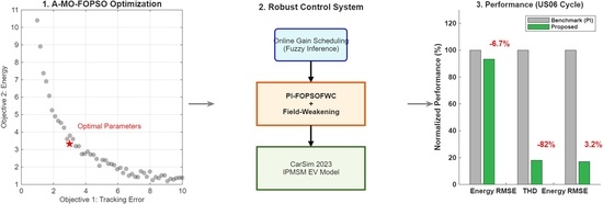
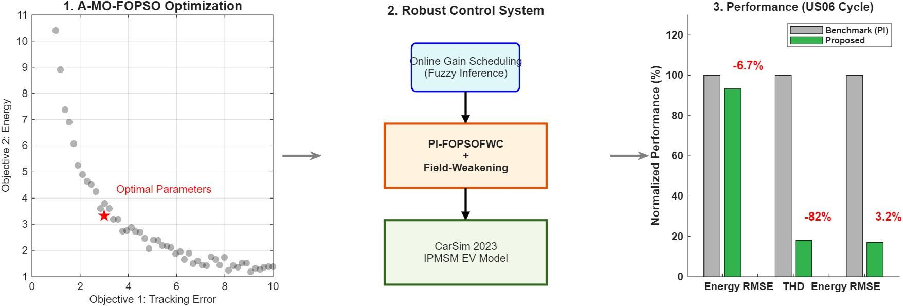
High-performance speed regulation of interior permanent magnet synchronous motor (IPMSM) drives in electric vehicle (EV) applications becomes particularly challenging in the field-weakening region, where voltage constraints, parameter variations, and nonlinear aerodynamic loads significantly affect the closed-loop stability. To address these challenges, this paper proposes a stability-aware adaptive fractional-order speed control framework for EV traction systems. The framework integrates a fractional-order PI (FOPI) core to provide iso-damping robustness, a bounded fuzzy gain-scheduling mechanism for real-time adaptation, and an offline multi-objective optimization layer for systematic parameter tuning. A Lyapunov-based qualitative analysis is provided to justify closed-loop ultimate boundedness under adaptive gain modulation and field-weakening constraints. The fuzzy scheduler is explicitly structured to regulate the error energy dissipation rate by modulating the proportional and integral gains while preserving the gain boundedness. The controller parameters are optimized using a diversity-driven fractional-order multi-objective PSO algorithm to balance the tracking accuracy and control effort. The proposed framework was validated using a high-fidelity MATLAB/Simulink–CarSim 2023 co-simulation platform under the aggressive US06 driving cycle. The results demonstrated a zero-overshoot transient response, robustness against a 2.5× inertia mismatch, and sustained performance under flux-linkage and inductance variations in deep field-weakening operation. Compared with conventional PI-based strategies, the proposed approach reduced the speed RMSE by 82%, lowered the current THD from 18.5% to 3.2%, and reduced the cumulative DC-link current-squared index by 6.7%. These results validate the practical robustness and computational feasibility of the proposed stability-aware framework for EV traction control.

1. Introduction

Driven by stringent emission regulations and the rapid electrification of transportation, the interior permanent magnet synchronous motor (IPMSM) has become a dominant traction solution in modern electric vehicles (EVs) and hybrid electric vehicles (HEVs) due to its high power density, efficiency, and torque-to-inertia ratio [1,2,3].

Despite these advantages, achieving high-performance speed control in EV applications remains challenging. The traction system is inherently nonlinear and time-varying, operating under strict voltage and current constraints in the field-weakening (FW) region [4,5,6]. In addition, aerodynamic drag ($F_{aero}\propto v^2$), road load variations, parameter uncertainties, and sensor non-idealities further degrade the closed-loop stability and bandwidth [7,8,9]. While observer-based schemes can alleviate sensing limitations, they typically increase the computational complexity and parameter sensitivity [10,11].

The conventional proportional–integral (PI) controller within the field-oriented control (FOC) framework remains the industrial standard due to its simplicity. However, fixed-gain PI controllers lack adaptability to nonlinear EV dynamics and may suffer performance degradations under a parameter mismatch [12]. Advanced control strategies, including model-predictive control (MPC), sliding mode control (SMC), and intelligent adaptive schemes, have been proposed to enhance the robustness [13,14,15,16]. Nevertheless, these methods often involve a higher computational burden or robustness– complexity trade-offs that limit their practical deployment in embedded EV platforms.

Fractional-order control (FOC) has emerged as a promising alternative due to its additional loop-shaping flexibility and iso-damping property [17,18]. By generalizing integral and derivative orders to real numbers, fractional-order controllers preserve the phase margin under gain variations, thereby enhancing the robustness against plant uncertainties [19,20,21]. In parallel, adaptive paradigms such as gain-scheduled PI, model reference adaptive control (MRAC), and disturbance-observer-based methods have been investigated for electric drives. More recently, event-triggered and output-feedback adaptive schemes have been introduced to reduce the computational burden while maintaining formal stability guarantees [16,22]. Representative adva=nces include adaptive event-triggered tracking control via switching functions [23] and adaptive event-triggered output-feedback control using output information only [24], which provide rigorous Lyapunov-based frameworks.

Nevertheless, most of these adaptive strategies were developed under simplified plant assumptions and do not explicitly consider the severe inverter voltage constraints and field-weakening (FW) dynamics inherent in high-speed EV traction systems. In addition, few studies provide a unified framework that simultaneously (i) ensures bounded adaptive gain modulation, (ii) preserves fractional-order iso-damping robustness, and (iii) accounts for realistic multi-body vehicle load interactions. From an energy-system perspective, high-speed FW operation inherently increases the current magnitude, thereby elevating copper loss ($P_{\mathrm{cu}}\propto i^{2}R$), inverter thermal stress, and drivetrain energy dissipation. Excessive current ripple and suboptimal current trajectories may therefore compromise both the dynamic performance and the energy efficiency. This observation motivates a multi-objective formulation that explicitly balances the tracking precision and the current-related energy dissipation under voltage-constrained operation. Tuning fractional-order controller parameters ($K_p$, $K_i$, $\lambda$) constitutes a non-convex optimization problem. Metaheuristic algorithms such as particle swarm optimization (PSO) and its variants have been widely adopted [25,26,27]. However, standard PSO may suffer from premature convergence in multi-modal EV control landscapes [28,29]. Furthermore, single-objective optimization cannot adequately capture the trade-off between dynamic precision and energy-related indices [30].

Another limitation of existing studies lies in the validation methodology. Many controllers are verified using simplified Simulink models with idealized loads, which fail to represent realistic multi-body vehicle dynamics. High-fidelity co-simulation with dedicated vehicle platforms (e.g., CarSim) is therefore essential for evaluating controller performance under aggressive driving conditions and realistic road-load disturbances [31,32,33].

To address these control-theoretic and energy-relevant challenges, this paper proposes a stability-aware adaptive fractional-order speed control framework for IPMSM-based EVs operating in the field-weakening region. The framework integrates three coordinated layers: (i) a fractional-order PI (FOPI) core exploiting iso-damping robustness, (ii) a bounded fuzzy gain-scheduling mechanism enabling stability-preserving adaptive compensation, and (iii) an offline diversity-driven multi-objective optimization layer for systematic parameter tuning. Unlike purely heuristic adaptive designs, the proposed approach incorporates a Lyapunov-based qualitative analysis to justify practical ultimate boundedness under bounded disturbances and voltage-constrained operation.

2. System Modeling and Operational Constraints

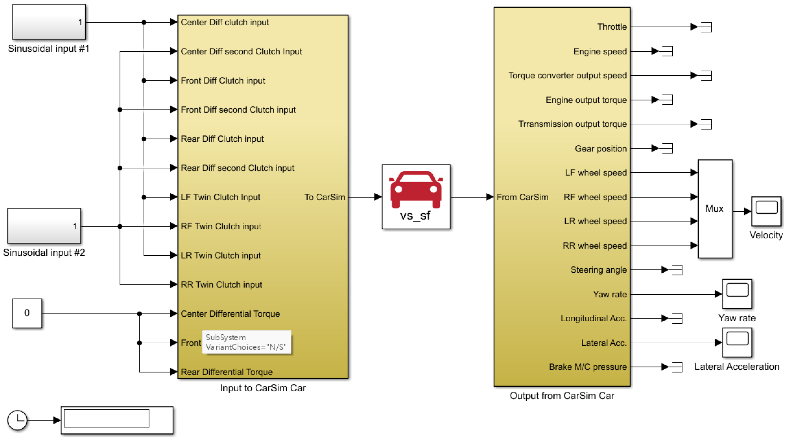
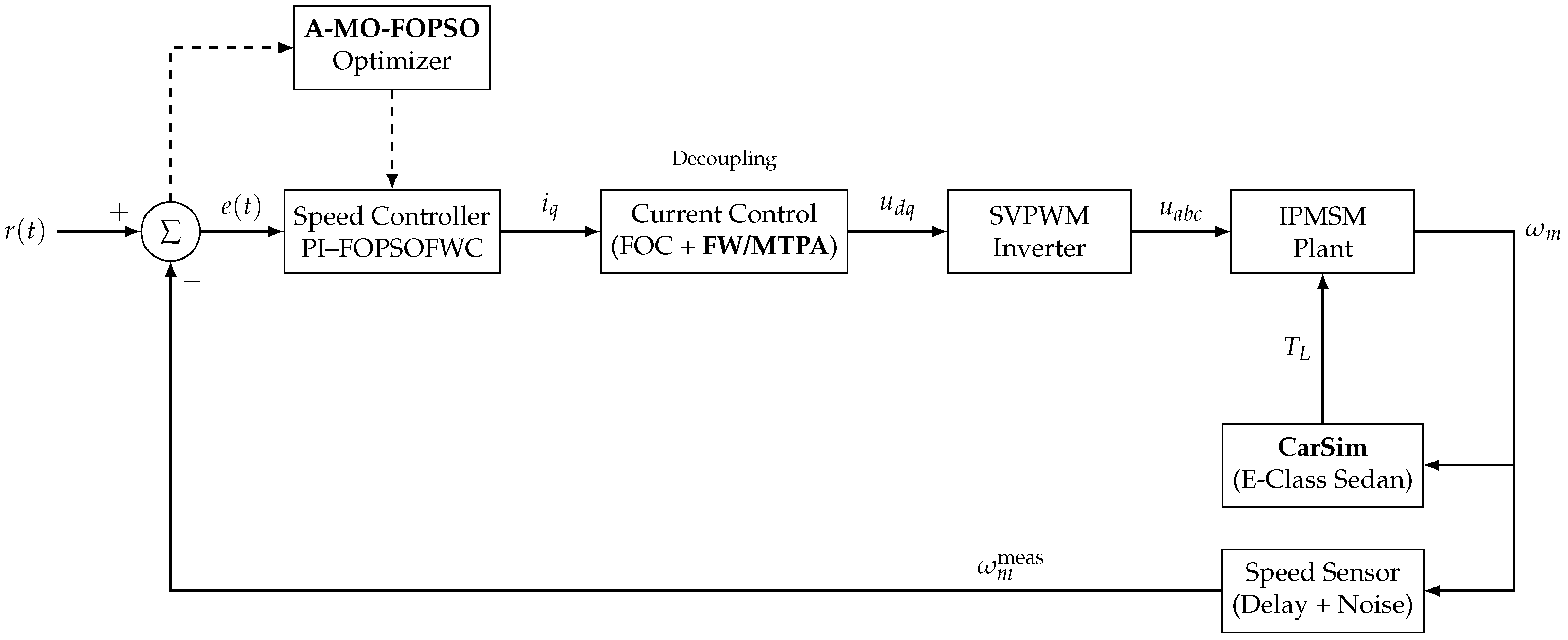
This section establishes the high-fidelity mathematical framework for the IPMSM traction drive system. To facilitate the multi-objective optimization of the efficiency and dynamic performance across the full speed range (including the field-weakening region), the model explicitly accounts for the inverter’s nonlinearities and physical constraints, as well as the complex vehicle dynamics provided by the CarSim 2023 co-simulation environment. The system architecture comprises four subsystems: the intelligent controller (FOPI + MOPSO), the power converter (VSI), the IPMSM traction motor, and the vehicle dynamics load. The interaction between the electrical and mechanical domains is validated using the synchronized co-simulation interface shown in Figure 1.

2.1. IPMSM Dynamic Model in $dq$-Reference Frame

The IPMSM is modeled in the synchronous rotating $dq$-reference frame. The stator voltage equations considering the cross-coupling effects are expressed as [3,12]:

$$\begin{array}{cc}\hfill v_d& =R_s{i}_d+L_d{\displaystyle \frac{d{i}_d}{dt}}-{\omega }_e{L}_q{i}_q,\hfill \\ \hfill v_q& =R_s{i}_q+L_q{\displaystyle \frac{d{i}_q}{dt}}+{\omega }_e(L_d{i}_d+{\psi }_f),\hfill \end{array}$$

(1)

where $v_{d,q}$ and $i_{d,q}$ represent the stator voltages and currents, $R_s$ is the stator resistance, $L_d$ and $L_q$ are the d- and q-axis inductances, and ${\omega }_e$ is the electrical angular velocity. ${\psi }_f$ denotes the permanent magnet flux linkage.

The electromagnetic torque $T_e$ is given by:

$$T_e={\displaystyle \frac{3}{2}}p\left({\psi }_f{i}_q+(L_d-L_q)i_d{i}_q\right),$$

(2)

where the second term captures the reluctance torque produced by rotor saliency ($L_d\ne L_q$). Here, p is the number of pole pairs. The mechanical dynamics, including the specific load torque $T_L$ from the vehicle, are governed by:

$$J{\displaystyle \frac{d{\omega }_m}{dt}}+B{\omega }_m=T_e-T_L,$$

(3)

where J is the system inertia, B is the viscous friction coefficient, and ${\omega }_m$ is the mechanical rotor speed.

Remark 1.

The inertia term J in Equation (3) denotes only the motor rotor inertia. The equivalent vehicle inertia reflected to the motor shaft is incorporated within the load torque term $T_L$ obtained from the CarSim co-simulation model. Therefore, no additional reflected inertia term is included in (3), avoiding double counting of the mechanical dynamics.

2.2. Power Converter and Nonlinearity Modeling

The voltage source inverter (VSI) was modeled considering both switching dynamics and physical non-idealities. The inverter is represented as a first-order lag with a time constant ${\tau }_s\approx$ 50 µs. To strictly evaluate the controller’s robustness against hardware limitations, the dead-time effect was explicitly modeled. The distorted phase voltage $v_{an}$ due to dead-time $T_{dead}$ is expressed as [34,35]:

$$v_{an}=v_{an}^{*}-\mathrm{sign}\left(i_a\right)·V_{dead},V_{dead}={\displaystyle \frac{T_{dead}}{T_{sw}}}{V}_{dc},$$

(4)

where $T_{sw}$ is the switching period. In this study, $T_{dead}$ = 2.0 µs and $f_{sw}$ = 20 kHz (i.e., $T_{sw}$ = 50 µs). Furthermore, to focus on the inverter’s nonlinear behavior and control limits, the DC-link voltage $V_{dc}$ was assumed to be provided by an ideal battery source with a constant magnitude, neglecting the voltage sag during high-power extraction.

2.3. Sensor Dynamics and Signal Non-Idealities

Accurate speed sensing is critical for the stability of the closed-loop system, particularly under the high-dynamic conditions of the US06 cycle. The sensor model in Figure 2 accounts for signal processing delays and measurement noise, which are often overlooked in simplified simulations. The measured speed ${\omega }_m^{\mathrm{meas}}$ is modeled as:

$${\omega }_m^{\mathrm{meas}}\left(s\right)={\displaystyle \frac{e^{-{\tau }_{d}s}}{1+{\tau }_{f}s}}{\omega }_m\left(s\right)+n\left(s\right),$$

(5)

where ${\tau }_d\approx$ 200 µs represents the cumulative communication and processing latency, ${\tau }_f$ is the time constant of the anti-aliasing filter, and $n\left(s\right)$ represents additive Gaussian white noise. This model challenges the controller to maintain tracking precision despite signal degradation.

2.4. Operational Constraints and Field-Weakening Strategy

Unlike conventional control studies that assume infinite voltage availability, this study specifically addresses the field-weakening (FW) operation required for highway cruising. The control algorithms are bounded by the inverter’s physical limits [4,5]:

2.4.1. Current and Voltage Limits

The stator current and voltage vectors are constrained by the inverter’s thermal rating $I_{max}$ and the DC-link voltage $V_{dc}$:

$$i_d^2+i_q^2\le I_{max}^2,v_d^2+v_q^2\le V_{max}^2={\left({\displaystyle \frac{V_{dc}}{\sqrt{3}}}\right)}^2.$$

(6)

2.4.2. Field-Weakening Control Strategy

To ensure seamless operation across the entire speed range, the reference d-axis current $i_d^{*}$ is determined based on the operating region:

• Constant Torque Region (MTPA): Below the base speed, the IPMSM operates under a maximum-torque-per-ampere strategy, where the optimal current reference typically requires a negative $i_d^{*}$ due to saliency ($L_d\ne L_q$).
• Field-Weakening Region: When the voltage limit is reached ($V_s\ge V_{max}$), $i_d^{*}$ is adjusted to maintain the voltage constraint. The analytical solution for the optimal flux-weakening current is derived as: (Under a steady-state high-speed approximation, the stator resistance and current derivative terms are neglected, yielding a closed-form reference based on the voltage-limit ellipse.)

  $$i_d^{*}=-{\displaystyle \frac{{\psi }_f}{L_d}}+\sqrt{{\displaystyle \frac{V_{max}^2}{{\left({\omega }_e{L}_d\right)}^2}}-{\left({\displaystyle \frac{L_q}{L_d}}{i}_q^{*}\right)}^2}.$$

  (7)

Remark 2.

Equation (7) provides a feasible closed-form reference on the voltage-limit boundary under the steady-state high-speed approximation. The final current commands are further shaped by the current-circle constraint in Equation (6) and the saturation/anti-windup logic in Figure 3 to ensure feasibility during field-weakening operation. This strategy ensures that the current vector trajectory tracks the voltage limit ellipse, maximizing the power capability at high speeds while preventing voltage saturation.

2.5. High-Fidelity Vehicle Load Modeling via CarSim

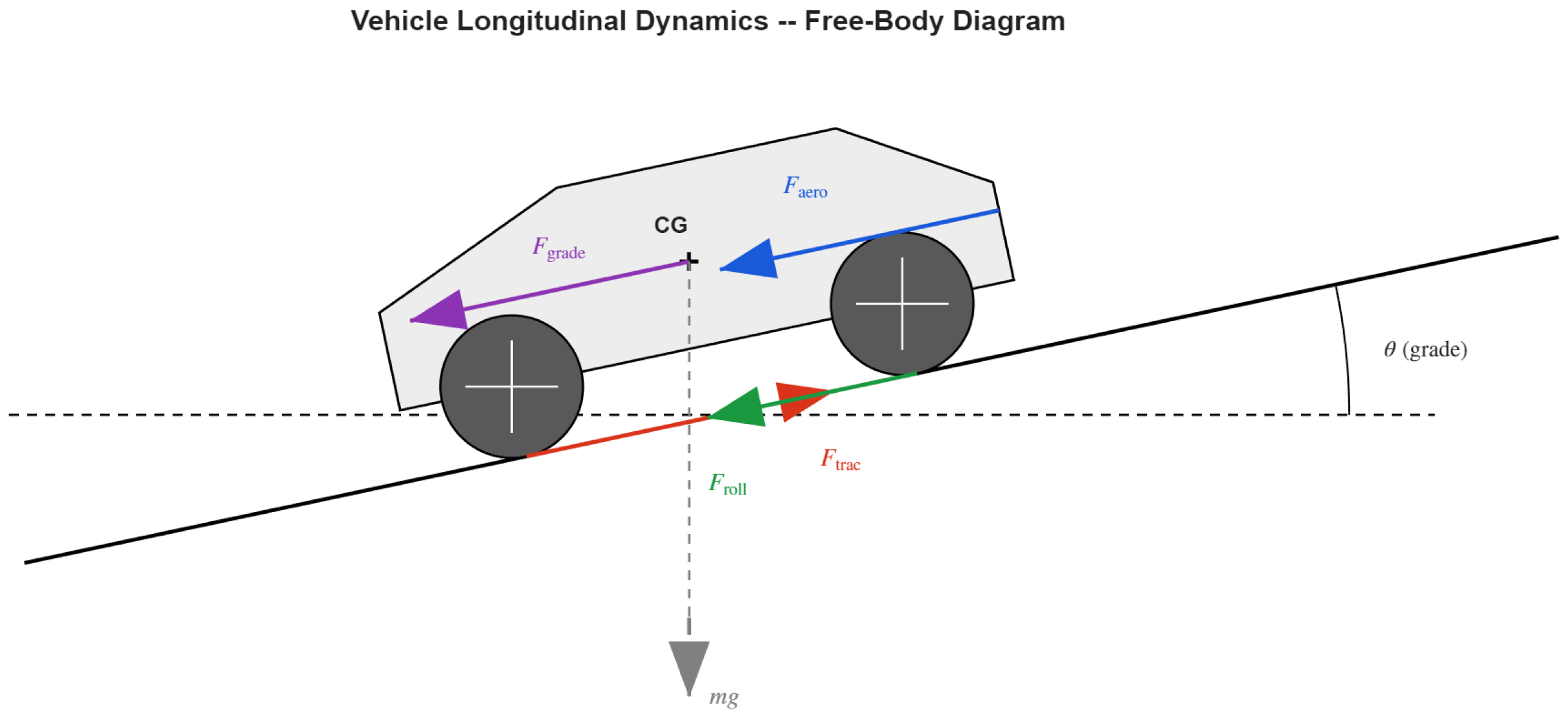
To ensure the research’s practical value for EV applications, this study moved beyond simplified load models. We utilized CarSim 2023 to simulate a high-fidelity E-class sedan model. The equivalent load torque $T_L$ reflected on the motor shaft is calculated dynamically based on the vehicle’s longitudinal dynamics, as illustrated by the free-body diagram in Figure 4 [32,36]:

$$T_L={\displaystyle \frac{r_{tire}}{G\eta }}\left(M_v{\displaystyle \frac{dv}{dt}}+F_{aero}\left(\alpha \right)+F_{roll}+F_{grade}\right),$$

(8)

where $F_{aero}\left(\alpha \right)$ represents the aerodynamic drag force, which is modeled as a function of the vehicle slip angle $\alpha$ using the predefined “drag vs. aero slip” characteristic map within the CarSim vehicle database. Since the standard US06 acceleration test was performed on a flat surface, the road grade force was set to zero ($F_{grade}=0$) in this simulation.

Using the standard road-load formulation in [7] together with the vehicle parameters in

Table 1. System parameters of the IPMSM drive and the target E-class sedan.

Parameter	Symbol	Value
IPMSM Parameters
Stator Resistance	$R_s$	$0.5\Omega$
$d/q$-axis Inductance	$L_d,L_q$	$5.0,6.0\mathrm{mH}$
Flux Linkage	${\psi }_f$	$0.1\mathrm{Wb}$
Inertia (Rotor Only)	J	$0.01\mathrm{kg}·{\mathrm{m}}^2$
Pole Pairs	p	4
Vehicle Parameters (CarSim E-Class Sedan)
Vehicle Mass	$M_v$	$1650\mathrm{kg}$
Effective Tire Radius	$r_{\mathrm{tire}}$	$0.35\mathrm{m}$
Aerodynamic Drag Coeff.	$C_d$	$0.30$ (Slip-Dependent)
Frontal Area	$A_f$	$2.4{\mathrm{m}}^2$
Transmission Gear Ratio	G	$9.5$
Drivetrain Efficiency	$\eta$	$97\%$
Test Cycle	-	US06 Acceleration

(with $F_{grade}=0$), we computed that the aerodynamic drag term accounts for approximately 65% of the total road load at 120 km/h under the considered operating condition. This highlights the quadratic load growth ($F_{aero}\propto v^2$) and motivates accurate field-weakening control to avoid voltage saturation and torque collapse at high velocities. It is worth noting that, while standard 1D longitudinal models (e.g., standard Simulink/Simscape EV blocks) are sufficient for basic controller tuning under constant loads, they often oversimplify the tire–road interactions and multi-body dynamics. Under highly aggressive driving cycles like US06, the vehicle experiences dynamic weight transfer and varying tire slip angles, which introduce significant nonlinearities into the aerodynamic drag (as modeled by the drag vs. aero slip map in CarSim) and rolling resistance. Co-simulation is therefore strictly necessary to capture these high-frequency, nonlinear load torque ($T_L$) fluctuations that directly impact the field-weakening stability. Furthermore, regarding the chosen Mercedes E-class sedan model, this study adopted its exact mechanical chassis parameters (e.g., 1650 kg mass, specific frontal area, and aerodynamic coefficients) to construct a realistic, heavy-load challenge for the IPMSM traction drive, rather than replicating its specific commercial hybrid energy management system (e.g., the W214 48V mild-hybrid architecture).

2.6. System Architecture

The overall closed-loop control structure is illustrated in Figure 2. The system incorporates the MOPSO optimizer for offline tuning and an inner current loop integrated with field-weakening (FW) logic to handle the high-speed dynamics of the E-class sedan.

To enforce practical inverter limits, the commanded currents are saturated within the current circle $i_d^{*2}+i_q^{*2}\le I_{max}^2$, and the commanded voltages are limited by $V_{max}=V_{dc}/\sqrt{3}$. When saturation occurs, an anti-windup strategy is applied to the (fractional) integrator (conditional integration/back-calculation) to prevent integrator windup and to maintain stable transients. In the field-weakening region, the $i_d^{*}$ reference is prioritized to satisfy the voltage constraint, while $i_q^{*}$ is adjusted accordingly.

2.7. Simulation Environment and Parameters

The co-simulation was executed in MATLAB/Simulink R2023 coupled with CarSim 2023. The solver step size was fixed at 50 µs. The key parameters for the IPMSM drive and the target E-class sedan are listed in Table 1. The vehicle mass (1650 kg) and high-speed aerodynamic characteristics pose a significantly greater challenge for energy optimization compared to compact EVs.

3. Robust Fractional-Order Control Strategy

This section presents the design of the proposed PI-based fractional-order PSO-fuzzy weight controller (PI-FOPSOFWC). To address the complex dynamics of the E-class EV model under the US06 driving cycle—specifically the nonlinear friction variations and parameter drifts in the field-weakening region—the control strategy integrates three layers: (1) a fractional-order PI (FOPI) core for structural robustness, (2) a fuzzy logic mechanism for online gain scheduling, and (3) an offline multi-objective optimization (MOPSO) layer for optimal parameter tuning.

3.1. Control Architecture and FOPI Core

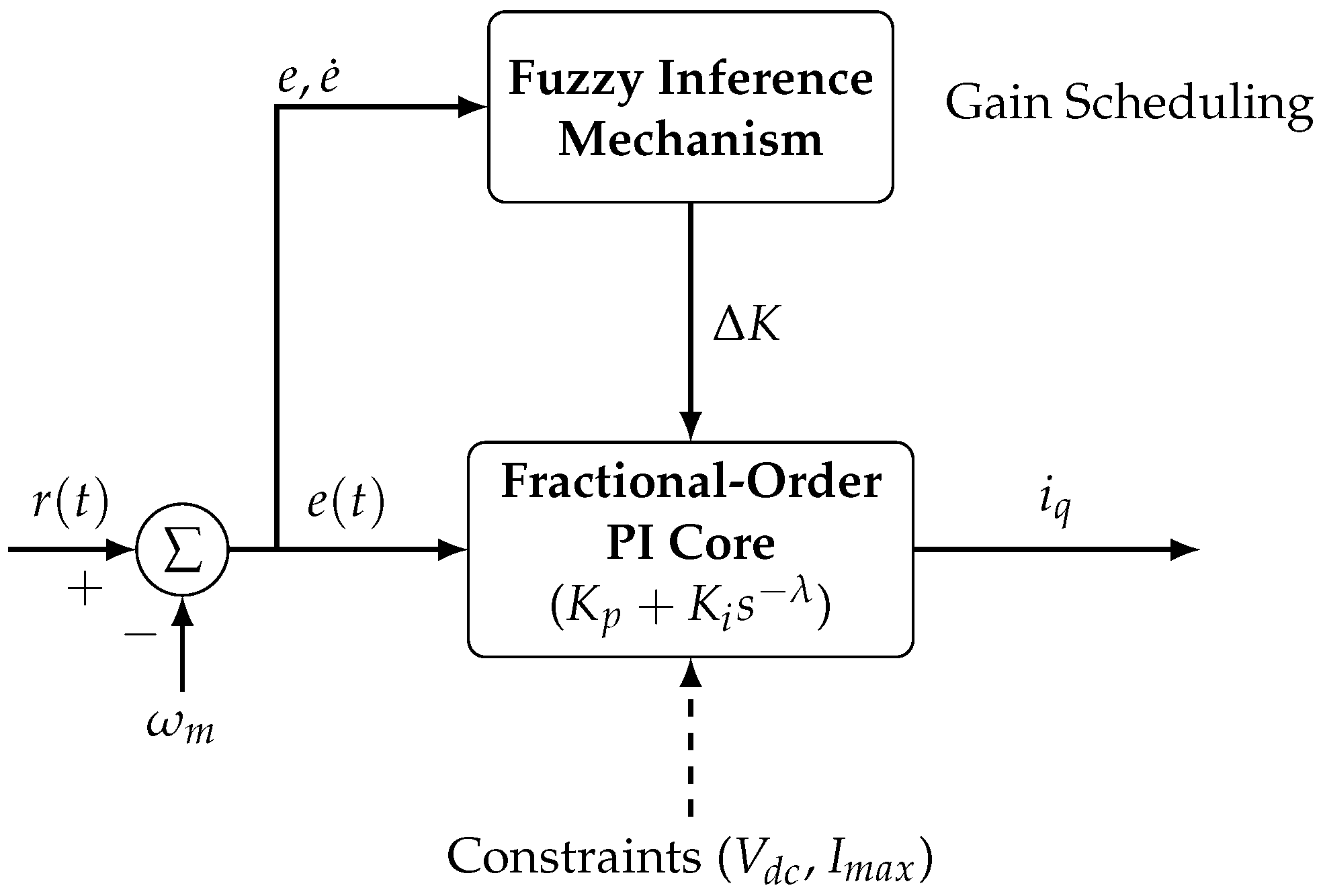
The detailed internal structure of the proposed controller is illustrated in Figure 3. The controller generates the torque-producing current reference $i_q^{*}$ based on the speed tracking error $e\left(t\right)=r\left(t\right)-{\omega }_m^{\mathrm{meas}}\left(t\right)$. Here, $r\left(t\right)$ denotes the speed reference, and ${\omega }_m^{\mathrm{meas}}\left(t\right)$ is the measured (delayed/noisy) speed signal used by the controller.

Unlike integer-order controllers, the FOPI controller introduces a fractional integration order $\lambda$, defined by the transfer function: 0

$$G_c\left(s\right)=K_p+K_i{s}^{-\lambda },(0<\lambda <2).$$

(9)

3.1.1. Iso-Damping Property

The primary motivation for employing FOPI is its “iso-damping” property. In the field-weakening region, the effective motor parameters vary due to magnetic saturation and cross-coupling. The FOPI controller is tuned to ensure the phase of the open-loop transfer function $L\left(s\right)$ is locally flat around the gain crossover frequency ${\omega }_{gc}$ [18,19]:

$${\displaystyle \frac{d\angle L\left(j\omega \right)}{d\omega }}{|}_{\omega ={\omega }_{gc}}\approx 0.$$

(10)

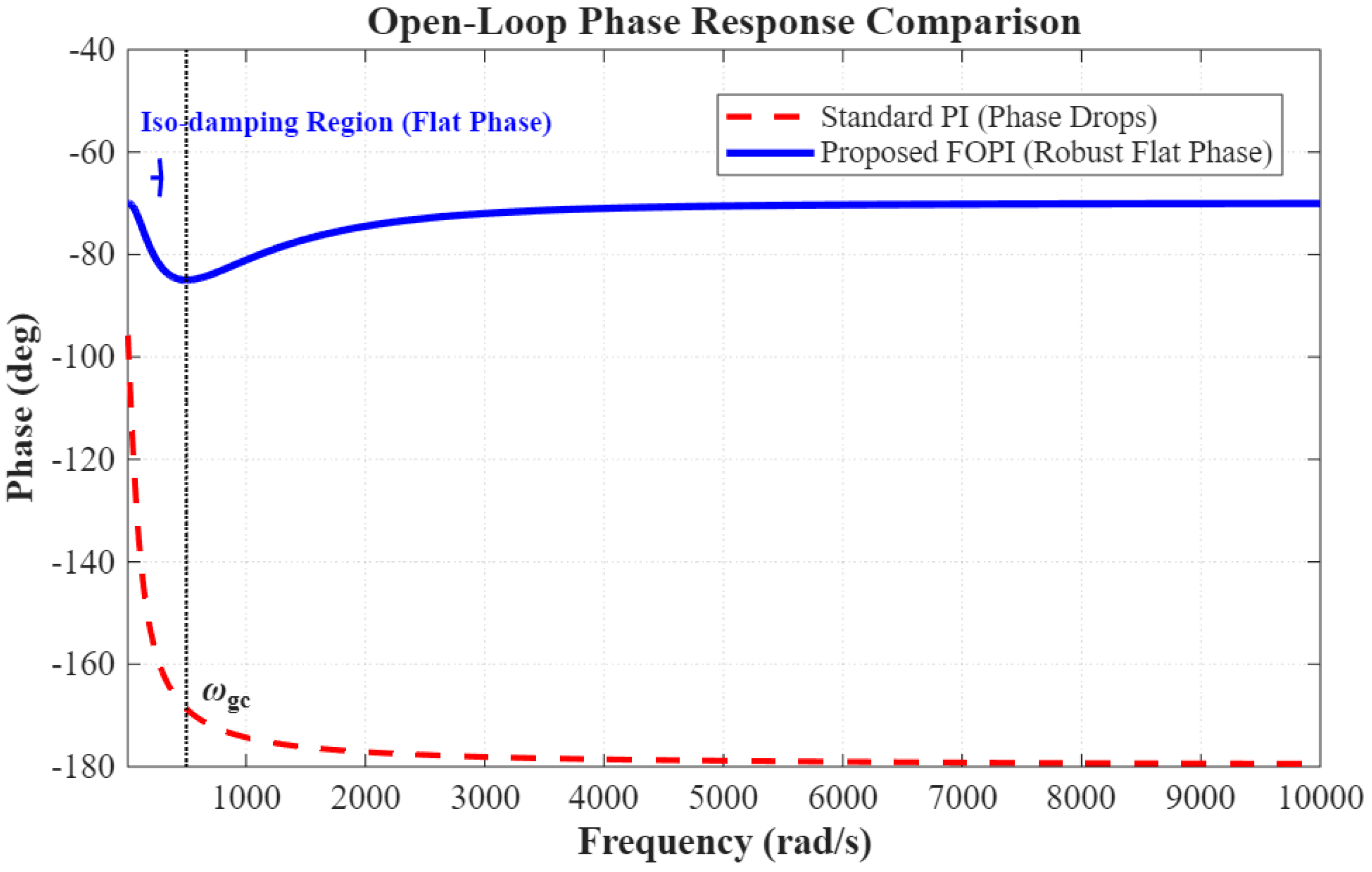
This ensures that the system’s phase margin (and consequently, the overshoot) remains robustly constant, despite variations in the plant gain.

3.1.2. Digital Implementation via Oustaloup Filter

For digital realization on an embedded controller, the fractional operator $s^{-\lambda }$ is approximated by the Oustaloup recursive approximation (ORA) within a predefined frequency band $[{\omega }_b,{\omega }_h]$ [37]. In this work, the ORA-based implementation was realized and verified using the FOMCON toolbox [38]. In this study, a filter order of $N=5$ was selected to balance the approximation accuracy and computational load. The resulting continuous transfer function was then discretized using the Tustin transformation ($s\approx {\displaystyle \frac{2}{T_s}}{\displaystyle \frac{z-1}{z+1}}$) for real-time execution in the simulation environment.

3.1.3. Membership Functions and Rule Base

Triangular membership functions are adopted for the fuzzy inference system (FIS) due to their low computational cost and suitability for real-time implementation. The FIS uses two inputs, namely the speed tracking error and its rate,

$$e\left(t\right)=r\left(t\right)-{\omega }_m^{\mathrm{meas}}\left(t\right),\dot{e}\left(t\right)={\displaystyle \frac{d}{dt}}e\left(t\right),$$

(11)

and produces two outputs for online gain adaptation, i.e., $(\Delta K_p,\Delta K_i)$.

• Normalization
  To make the membership functions independent of the absolute magnitude of the driving cycle and to facilitate universal tuning, the inputs are normalized to the domain $[-1,1]$ as

  $$\tilde{e}\left(t\right)=\mathrm{sat}\left({\displaystyle \frac{e\left(t\right)}{E_{max}}}\right),\tilde{\dot{e}}\left(t\right)=\mathrm{sat}\left({\displaystyle \frac{\dot{e}\left(t\right)}{{\dot{E}}_{max}}}\right),$$

  (12)

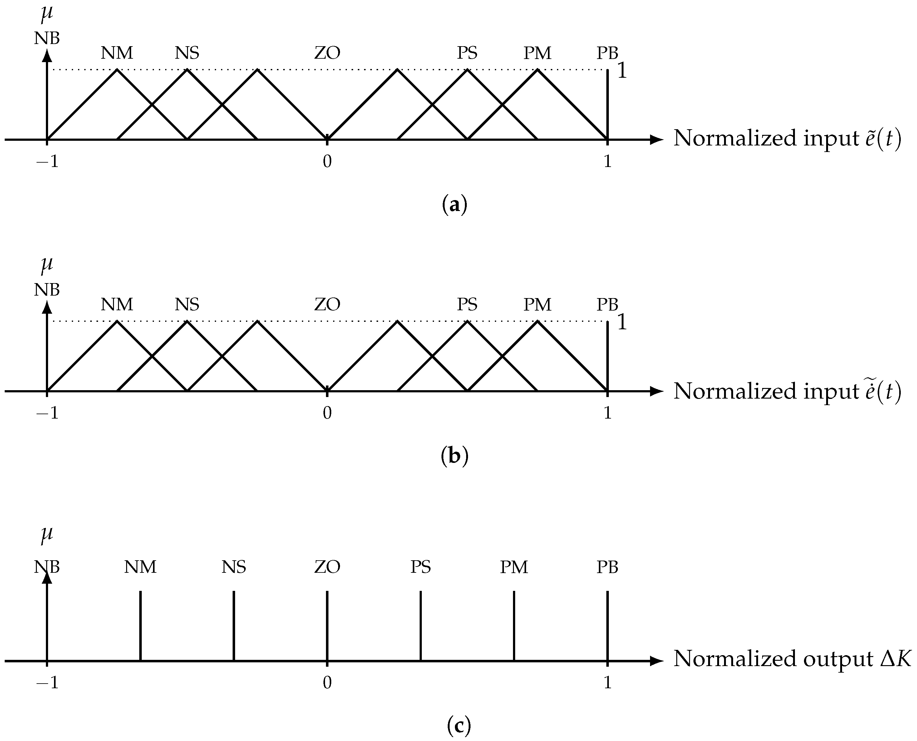
  where $\mathrm{sat}\left(x\right)=max(-1,min(1,x\left)\right)$, and $E_{max}$ and ${\dot{E}}_{max}$ are normalization bounds selected according to the expected maximum speed error and error rate in the US06 cycle. Hence, the center of the linguistic term ZO corresponds to the normalized value 0 (see Figure 5).
• Membership Functions
  Seven linguistic terms were employed for each normalized input: $\{\mathrm{NB},\mathrm{NM},\mathrm{NS},\mathrm{ZO},\mathrm{PS},\mathrm{PM},\mathrm{PB}\}$ (negative big to positive big), distributed symmetrically over $[-1,1]$. Figure 5a,b illustrates the membership functions for $\tilde{e}\left(t\right)$ and $\tilde{\dot{e}}\left(t\right)$, respectively. For the gain-adjustment output, a singleton-type linguistic set was adopted (Figure 5c) that is computationally efficient and commonly used for real-time fuzzy gain scheduling.
• Gain Adaptation Law
  The controller gains are updated online as

  $$K_p\left(t\right)=K_{p0}+{\alpha }_p\Delta K_p\left(\tilde{e},\tilde{\dot{e}}\right),K_i\left(t\right)=K_{i0}+{\alpha }_i\Delta K_i\left(\tilde{e},\tilde{\dot{e}}\right),$$

  (13)

  where $(K_{p0},K_{i0})$ are the nominal gains and $({\alpha }_p,{\alpha }_i)$ are scaling factors optimized by MOPSO. Here, $\Delta K_p$ and $\Delta K_i$ are dimensionless outputs of the FIS in the normalized range $[-1,1]$.
• Rule Base and Inference
  The fuzzy rules were designed based on the distinct physical roles of the proportional and integral terms in EV traction control.

  1.

  Proportional Gain ($K_p$): The rule base for $\Delta K_p$ is presented in

  Table 2. Fuzzy rule base for proportional gain adaptation (output: $\Delta K_p$).

  $\widetilde{\dot{\mathit{e}}}$	$\tilde{\mathit{e}}$
  	NB	NM	NS	ZO	PS	PM	PB
  NB	PB	PB	PM	PM	PS	ZO	ZO
  NM	PB	PM	PM	PS	ZO	NS	NS
  NS	PM	PM	PS	ZO	NS	NM	NM
  ZO	PM	PS	ZO	ZO	ZO	NS	NM
  PS	NM	NS	ZO	ZO	PS	PM	PM
  PM	NM	NM	NS	ZO	PM	PM	PB
  PB	ZO	ZO	PS	PM	PM	PB	PB

  . The logic follows a standard “large error, large gain” principle. When the error magnitude $|\tilde{e}|$ is large (e.g., NB or PB), a large positive adjustment (PB/PM) is applied to maximize the bandwidth. Conversely, when the system is near steady-state (ZO), $\Delta K_p$ is reduced to minimize the noise sensitivity.

  2.

  Integral Gain ($K_i$): The rule base for $\Delta K_i$ is presented in

  Table 3. Fuzzy rule base for integral gain adaptation (output: $\Delta K_i$).

  $\widetilde{\dot{\mathit{e}}}$	$\tilde{\mathit{e}}$
  	NB	NM	NS	ZO	PS	PM	PB
  NB	NB	NB	NM	NM	NS	ZO	ZO
  NM	NB	NM	NM	NS	ZO	PS	PS
  NS	NM	NM	NS	ZO	PS	PM	PM
  ZO	NM	NS	ZO	ZO	ZO	PS	PM
  PS	PM	PS	ZO	ZO	NS	NM	NM
  PM	PM	PM	PS	ZO	NM	NM	NB
  PB	ZO	ZO	NS	NM	NM	NB	NB

  . To prevent integrator windup, inverse adaptation logic was employed. When the error was large, $\Delta K_i$ was significantly reduced (NB/NM) to dampen the overshoot. $\Delta K_i$ was maintained at a nominal level or increased only when the error converged to zero (ZO) to eliminate steady-state error.

A Mamdani-type inference engine with a standard min–max composition was employed, and the crisp outputs $(\Delta K_p,\Delta K_i)$ were obtained using center-of-gravity (CoG) defuzzification.

3.1.4. Stability-Aware Design via Lyapunov Insight

To provide theoretical insight into the stability properties of the proposed adaptive fractional-order speed controller under field-weakening operation, a Lyapunov-based qualitative analysis is presented. Let the speed tracking error be defined as $e\left(t\right)=r\left(t\right)-{\omega }_m^{meas}\left(t\right)$. Consider the positive-definite Lyapunov candidate function:

$$V\left(t\right)={\displaystyle \frac{1}{2}}e{\left(t\right)}^2$$

(14)

The time derivative is given by

$$\dot{V}\left(t\right)=e\left(t\right)\dot{e}\left(t\right)$$

(15)

The closed-loop error dynamics of the IPMSM speed loop can be abstractly expressed as

$$\dot{e}\left(t\right)=-a\left(t\right)e\left(t\right)+d\left(t\right)$$

(16)

where $a\left(t\right)$ represents the equivalent adaptive feedback gain resulting from $K_p\left(t\right)$ and $K_i\left(t\right)$, and $d\left(t\right)$ captures bounded disturbances induced by load torque variations and parameter uncertainties in the field-weakening region. Since the fuzzy inference outputs $\Delta K_p$ and $\Delta K_i$ are confined within $[-1,1]$, and the scaling factors ${\alpha }_p$ and ${\alpha }_i$ are bounded by design, the adaptive gains $K_p\left(t\right)$ and $K_i\left(t\right)$ remain bounded. Therefore, $a\left(t\right)$ is strictly positive and bounded within a finite interval. The fuzzy rule base is explicitly structured to increase $K_p\left(t\right)$ when $e\dot{e}>0$ (diverging phase), thereby increasing $a\left(t\right)$ and promoting faster error energy dissipation. Conversely, when $e\dot{e}<0$ (converging phase), $K_p\left(t\right)$ is reduced to prevent excessive damping and overshoot, while $K_i\left(t\right)$ is moderately adjusted to eliminate steady-state error under aerodynamic load $F_{aero}\propto v^2$. Under these bounded-gain conditions and assuming bounded disturbance $d\left(t\right)$, the error dynamics satisfy the standard form of a first-order system with bounded perturbation. Hence, $\dot{V}\left(t\right)$ becomes negative outside a compact neighborhood of the origin, indicating practical ultimate boundedness of the tracking error. The fractional-order stability interpretation is consistent with the standard Mittag–Leffler stability framework under bounded adaptive gains. Although a full fractional-order stability proof is beyond the scope of this paper, the bounded adaptive gains together with the first-order error structure ensure practical ultimate boundedness under standard EV traction operating conditions.

3.2. Design Variables for Optimization

The performance depends on the optimal selection of the base parameters. The decision vector $\mathbf{x}$ is defined as:

$$\mathbf{x}={[K_{p0},K_{i0},\lambda ,{\alpha }_p,{\alpha }_i]}^T.$$

(17)

These parameters are tuned offline using the MOPSO framework detailed in Section 4 to balance the conflicting objectives of the tracking accuracy and energy efficiency.

4. Multi-Objective Optimization Strategy

The design of a robust controller for EV traction drives involves inherent trade-offs. A high-gain controller provides fast tracking and disturbance rejection, but often leads to an excessive control effort, increasing the inverter thermal stress and reducing the battery efficiency. Conversely, a low-gain controller saves energy, but compromises the transient performance. To address these conflicting goals, this study employed a multi-objective fractional-order particle swarm optimization (MO-FOPSO) framework. By introducing fractional calculus into the particle velocity update, the proposed algorithm mitigates the premature convergence often observed in standard PSO, ensuring a more diverse exploration of the Pareto front.

4.1. Problem Formulation

The optimization problem was formulated to simultaneously minimize two conflicting objective functions, $f_1\left(\mathbf{x}\right)$ and $f_2\left(\mathbf{x}\right)$, subject to the operational constraints defined in Section 2.4.

4.1.1. Objective 1: Dynamic Tracking Performance

To quantify the tracking precision and settling speed, the integral of time-weighted absolute error (ITAE) was selected. The time weighting penalizes long-duration errors, ensuring fast convergence:

$$f_1\left(\mathbf{x}\right)={\int }_0^{T_{sim}}t·|r\left(t\right)-{\omega }_m^{\mathrm{meas}}\left(t\right)|dt.$$

(18)

4.1.2. Objective 2: Control Effort (Energy-like Index)

To reduce actuator stress and current-related losses, the second objective is defined as an energy-like control-effort index based on the squared torque-producing current reference:

$$f_2\left(\mathbf{x}\right)={\int }_0^{T_{sim}}{\left[i_q^{*}\left(t\right)\right]}^{2}dt.$$

(19)

Although $f_2$ does not directly correspond to the physical energy consumption, it is proportional to the copper-loss component ($P_{\mathrm{cu}}\propto i^{2}R$). Therefore, minimizing $f_2$ indirectly reduces copper loss and inverter thermal stress, which are critical factors in EV energy efficiency and the component lifetime. Hence, it serves as a practical surrogate index for current-related energy dissipation and inverter stress in EV traction drives. The d-axis current component is not included in $f_2$, as it is primarily governed by the MTPA/field-weakening (FW) strategy and constrained by the inverter voltage limit. The optimization vector $\mathbf{x}={[K_{p0},K_{i0},\lambda ,{\alpha }_p,{\alpha }_i]}^T$ is bounded by the search space $\Omega$: ${\mathbf{x}}_{min}\le \mathbf{x}\le {\mathbf{x}}_{max}$.

4.2. Proposed MO-FOPSO Algorithm

Unlike single-objective optimization, which seeks a single global optimum, MO-FOPSO seeks a set of Pareto-optimal solutions. A solution ${\mathbf{x}}_1$ dominates ${\mathbf{x}}_2$ (denoted as ${\mathbf{x}}_1\prec {\mathbf{x}}_2$) if $f_i\left({\mathbf{x}}_1\right)\le f_i\left({\mathbf{x}}_2\right)$ for all objectives and $f_j\left({\mathbf{x}}_1\right)<f_j\left({\mathbf{x}}_2\right)$ for at least one objective. To enhance the global search capability, the standard velocity update is modified using the fractional derivative concept. Unlike conventional multi-objective PSO implementations that rely on static inertia weight-reduction schedules, the proposed diversity-feedback mechanism dynamically adjusts the exploration intensity based on population dispersion.

4.2.1. Fractional-Order Velocity Update

Standard PSO relies on integer-order velocity memory (order $\alpha =1$), which can lead to rapid loss of diversity. The proposed algorithm utilizes a fractional derivative of order $\alpha \in (0,1)$ to introduce a “long-term memory” effect. The discrete-time implementation using the Grünwald–Letnikov (G-L) approximation is given by:

$$v_{i,d}^{k+1}=w^k\underset{\mathrm{Fractional}\mathrm{Memory}}{\underbrace{\sum _{r=0}^M{(-1)}^r\left({\displaystyle \genfrac{}{}{0pt}{}{\alpha }{r}}\right)v_{i,d}^{k-r}}}+c_1^k{r}_1(p_{i,d}^{best}-x_{i,d}^k)+c_2^k{r}_2(g_{archive,d}^k-x_{i,d}^k),$$

(20)

where M is the memory length; $r_1,r_2\in [0,1]$ are uniformly distributed random numbers; and the binomial coefficients $\left({\displaystyle \genfrac{}{}{0pt}{}{\alpha }{r}}\right)$ effectively weight historical velocities. This term acts as a damper, preventing particles from stagnating in local optima.

Selection of Fractional Order $\alpha$

In this study, the fractional velocity order $\alpha$ was empirically set to $0.6$. A preliminary sensitivity analysis indicated that $\alpha <0.4$ resulted in an insufficient memory effect and a reduced exploration capability, whereas $\alpha >0.8$ may introduce excessive oscillatory behavior in the velocity update. The selected value $\alpha =0.6$ provides a balanced trade-off between long-term memory retention and numerical stability, ensuring smooth convergence while preserving swarm diversity.

4.2.2. Diversity-Driven Adaptive Parameter Scheduling

In the context of EV traction drives, particularly in the field-weakening region, the objective function landscape becomes highly multi-modal due to voltage constraints and magnetic saturation. Standard PSO often gets trapped in local optima under these conditions. To address this, a swarm diversity indicator is computed at each iteration using the population size N:

$$D^k={\displaystyle \frac{1}{N}}\sum _{i=1}^N{\displaystyle \frac{{∥{\mathbf{x}}_i^k-{\overline{\mathbf{x}}}^k∥}_2}{{∥{\mathbf{x}}_{max}-{\mathbf{x}}_{min}∥}_2}},{\overline{\mathbf{x}}}^k={\displaystyle \frac{1}{N}}\sum _{i=1}^N{\mathbf{x}}_i^k.$$

(21)

The normalized diversity is defined as ${\tilde{D}}^k=min(1,max(0,D^k))$. Using ${\tilde{D}}^k$ as feedback, the PSO coefficients in (20) are updated as:

$$w^k=w_{min}+\left(w_{max}-w_{min}\right)\left(1-{\tilde{D}}^k\right),$$

(22)

$$c_1^k=c_{1,min}+\left(c_{1,max}-c_{1,min}\right){\tilde{D}}^k,c_2^k=c_{2,min}+\left(c_{2,max}-c_{2,min}\right){\tilde{D}}^k.$$

(23)

This schedule increases exploration (larger $w^k$) when the swarm becomes overly concentrated (small ${\tilde{D}}^k$), and emphasizes convergence when the swarm remains well spread. For numerical smoothness, an exponential filter is applied: ${\theta }^k\leftarrow \rho {\theta }^{k-1}+(1-\rho ){\theta }^k$ with $\rho =0.8$ and $\theta \in \{w,c_1,c_2\}$. In this work, the bounds were set as $w\in [0.4,0.9]$ and $c_{1,2}\in [1.5,2.5]$.

4.2.3. Archive and Leader Selection

The algorithm maintains an external archive to store non-dominated solutions found during the search.

• Grid-Based Maintenance: To prevent the archive from growing indefinitely, an adaptive grid mechanism is used. When the archive is full, solutions in crowded regions are removed to maintain diversity.
• Leader Selection ($g_{best}$): The global guide for each particle is not fixed. It is selected from the archive using a roulette wheel selection based on the crowding distance, encouraging particles to explore sparse regions of the Pareto front.

4.3. Best Compromise Solution Selection

Upon completion, the algorithm produces a Pareto front. To select the final controller configuration, a fuzzy decision-making approach is applied. A linear membership function ${\mu }_i^k$ is assigned to the k-th solution for the i-th objective:

$${\mu }_i^k=\left\{\begin{array}{cc}1,\hfill & f_i^k\le f_i^{min}\hfill \\ {\displaystyle \frac{f_i^{max}-f_i^k}{f_i^{max}-f_i^{min}}},\hfill & f_i^{min}<f_i^k<f_i^{max}\hfill \\ 0,\hfill & f_i^k\ge f_i^{max}\hfill \end{array}\right.$$

(24)

The normalized optimality degree ${\mu }^k$ for each solution is calculated as:

$${\mu }^k={\displaystyle \frac{{\sum }_{i=1}^{N_{obj}}{\mu }_i^k}{{\sum }_{j=1}^{M_{arc}}{\sum }_{i=1}^{N_{obj}}{\mu }_i^j}}.$$

(25)

where $N_{obj}$ represents the number of objectives (here, $N_{obj}=2$) and $M_{arc}$ denotes the number of non-dominated solutions currently stored in the archive. The solution with the maximum ${\mu }^k$ provides the best trade-off between tracking accuracy and energy efficiency and is selected as the final controller design.

4.4. Optimization Flowchart

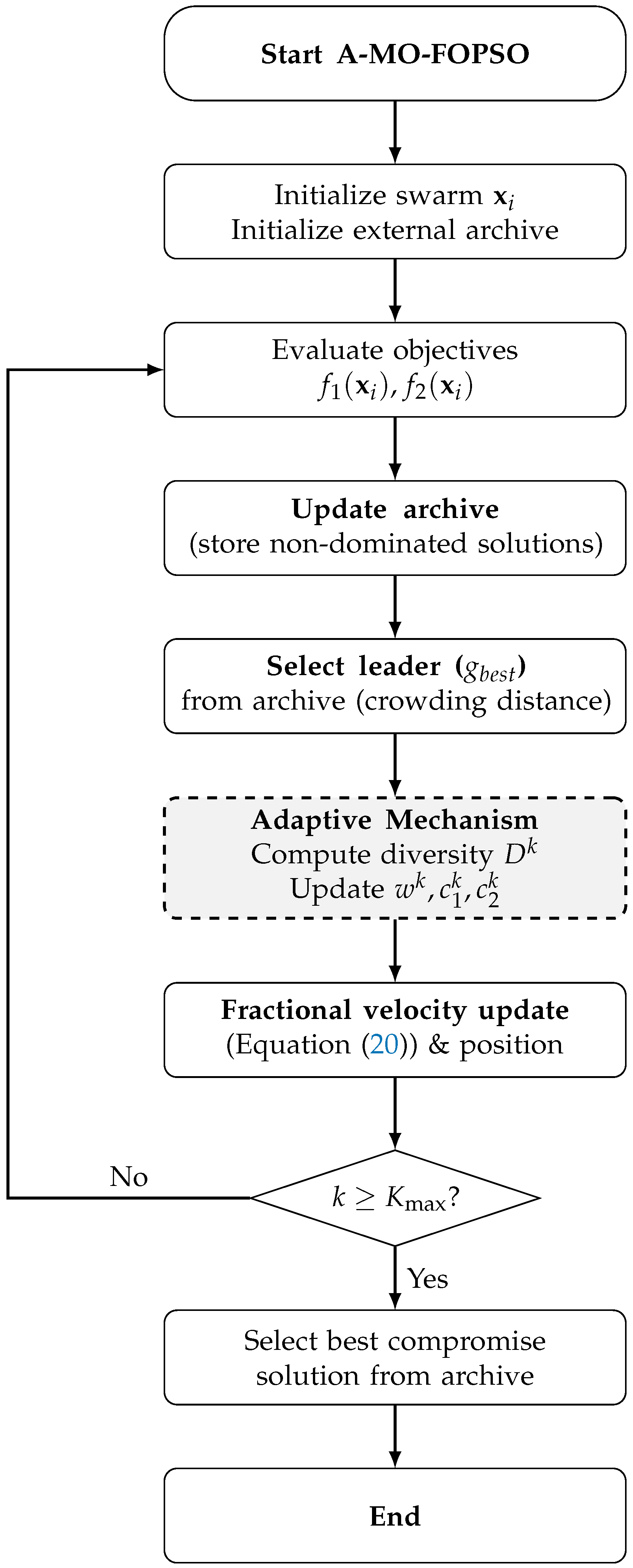
The complete execution flow of the proposed MO-FOPSO framework is illustrated in Figure 6.

4.5. Optimization Setup

The optimization process is executed offline. The key parameters configured for the MO-FOPSO algorithm are summarized in

Table 4. Configuration parameters and search space limits for MO-FOPSO.

Parameter Description	Symbol	Value/Range
A. MO-FOPSO Algorithm Settings
Population Size	N	50
Maximum Iterations	$K_{max}$	100
Archive Size	$N_{arc}$	100
Fractional Velocity Order	$\alpha$	0.6
Velocity Memory Length	M	4
Acceleration Coefficients	$c_1^k,c_2^k$	$[1.5,2.5]$ (adaptive)
Inertia Weight	$w^k$	$[0.4,0.9]$ (adaptive)
B. Decision Variable Search Space (Boundaries)
Nominal Proportional Gain	$K_{p0}$	$[0,100]$
Nominal Integral Gain	$K_{i0}$	$[0,100]$
Fractional Integration Order	$\lambda$	$[0.1,2.0]$
Fuzzy Scaling Factor (P)	${\alpha }_p$	$[0,5.0]$
Fuzzy Scaling Factor (I)	${\alpha }_i$	$[0,5.0]$

. The large number of generations ensures convergence of the fractional-order dynamics.

5. Simulation Results and Comparative Analysis

Among the evaluated cycles, US06 represents the most stringent high-speed and field-weakening stress scenario. WLTC and NEDC are included to validate the generalization capability. To rigorously validate the effectiveness of the proposed PI-FOPSOFWC strategy, comprehensive co-simulations were conducted using the high-fidelity platform established in Section 2. The simulation environment coupled MATLAB/Simulink R2023 with CarSim 2023 to replicate realistic EV dynamics. To establish a comprehensive performance hierarchy, the proposed method was benchmarked against three baselines:

1.

Baseline I (Std-PI): A standard integer-order PI controller tuned via the Ziegler–Nichols tuning rules [39], representing the industry standard.

2.

Baseline II (Fuzzy-PI): An integer-order fuzzy-PI controller optimized by standard MOPSO, representing a conventional intelligent control approach.

3.

Baseline III (Fixed-FOPSO): The proposed PI-FOPSOFWC tuned by a non-adaptive MO-FOPSO (fixed coefficients $w=0.7,c_1=c_2=2.0$). This baseline isolates the structural benefit of the fractional-order controller from the adaptive optimization mechanism.

4.

Proposed (A-MO-FOPSO): The complete strategy utilizing diversity-driven adaptive parameter scheduling.

The sampling frequency was 20 kHz. To ensure a high fidelity, the dead-time effect ($2.0$ µs) and sensor noise ($\sigma =10$ rpm) were activated in all scenarios. Around the nominal operating speed range of the US06 cycle, this corresponds to an equivalent SNR on the order of ∼20 dB. All baseline controllers were tuned to their respective best achievable performance to ensure fairness of comparison.

5.1. Phase 1: Optimization Performance Validation

First, the efficacy of the proposed MO-FOPSO algorithm was evaluated against the benchmarks. Both algorithms were executed with a population size of 50 for 100 iterations. For reproducibility, all optimization runs were performed with $N_s$ independent random seeds. The specific parameters of the selected “best compromise solution” (marked in Figure 7) are detailed in

Table 5. Optimized control parameters (best compromise solution).

Parameter	Symbol	Optimized Value
Nominal Proportional Gain	$K_{p0}$	2.15
Nominal Integral Gain	$K_{i0}$	45.20
Fractional Integration Order	$\lambda$	0.62
Fuzzy Scaling Factor (P)	${\alpha }_p$	0.85
Fuzzy Scaling Factor (I)	${\alpha }_i$	0.90
Computational Cost
Offline Optimization Time	$T_{opt}$	≈18 min
Est. Online Execution Time	$T_{exe}$	$3.2\mu$s

Note: The reported online execution time $T_{exe}$ estimates only the proposed speed-controller computations (FIS evaluation and ORA-based fractional operator with $N=5$), excluding PWM generation and peripheral I/O.

.

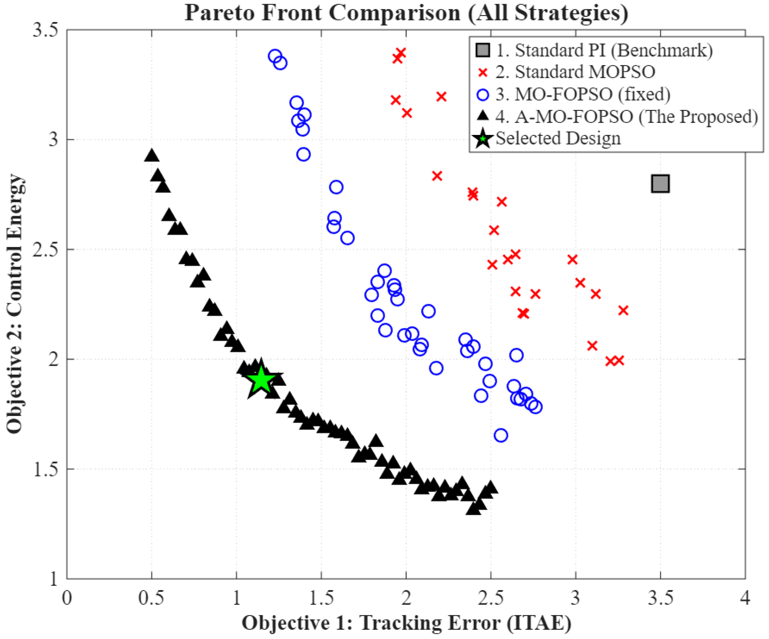
Figure 7 compares the final Pareto fronts. The horizontal axis represents the tracking performance objective ($f_1$: ITAE), and the vertical axis represents the control-effort objective ($f_2$: energy-like index).

• Benchmark Point: The standard PI (gray square) exhibited a high level of tracking error and energy consumption, serving as a poor reference point far from the origin.
• Diversity: The solutions found by MO-FOPSO (blue circles) and the proposed method (black triangles) were uniformly distributed along the front, whereas the standard MOPSO (red crosses) exhibited clustering. This superior diversity was attributed to the fractional-order velocity memory (Equation (20)) and the proposed diversity-driven adaptive coefficient scheduling.
• Convergence: The proposed A-MO-FOPSO front exhibited clear dominance over both the standard MOPSO and fixed-FOPSO fronts across most of the trade-off region.

The “best compromise solution” (marked with a green star) was selected for the subsequent control experiments.

5.2. Phase 2: Fundamental Time–Frequency Analysis

To investigate the fundamental control characteristics, the system was analyzed in both the time and frequency domains.

5.2.1. Step Response and Disturbance Rejection

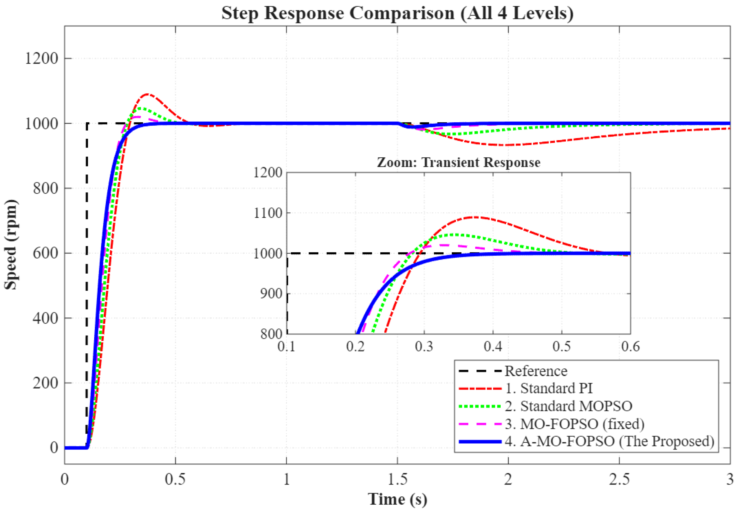
Figure 8 illustrates the speed response under a step command followed by a load disturbance ($T_L=50$ Nm). A clear hierarchical improvement was observed:

• Std-PI (Red): Suffered from significant overshoot ($8.5\%$) and a slow settling time due to integrator windup.
• Fuzzy-PI (Green) and Fixed-FOPSO (Magenta): Progressively reduced the overshoot to $4.2\%$ and $2.1\%$, respectively.
• Proposed (Blue): Achieved a critically damped-like response with negligible overshoot and the fastest settling time, verifying the effectiveness of adaptive tuning.

Figure 8. Speed response comparison (4 levels). The proposed controller eliminated overshoot and rejected disturbance more effectively than all baselines.

Figure 8. Speed response comparison (4 levels). The proposed controller eliminated overshoot and rejected disturbance more effectively than all baselines.

5.2.2. Frequency Domain Analysis (Iso-Damping)

The robustness observed in the time domain is theoretically supported by the frequency response shown in Figure 9. The standard PI controller exhibited a rapid phase drop near the crossover frequency ${\omega }_{gc}$. In contrast, the proposed FOPI controller maintained a “flat phase” characteristic (iso-damping region) around ${\omega }_{gc}$, ensuring that the system’s damping ratio remained constant despite parameter drifts.

5.3. Phase 3: Robustness Stress Testing

To further validate the robustness claims, the system was subjected to extreme parameter variations and signal non-idealities.

5.3.1. 3D Parameter Sensitivity Analysis

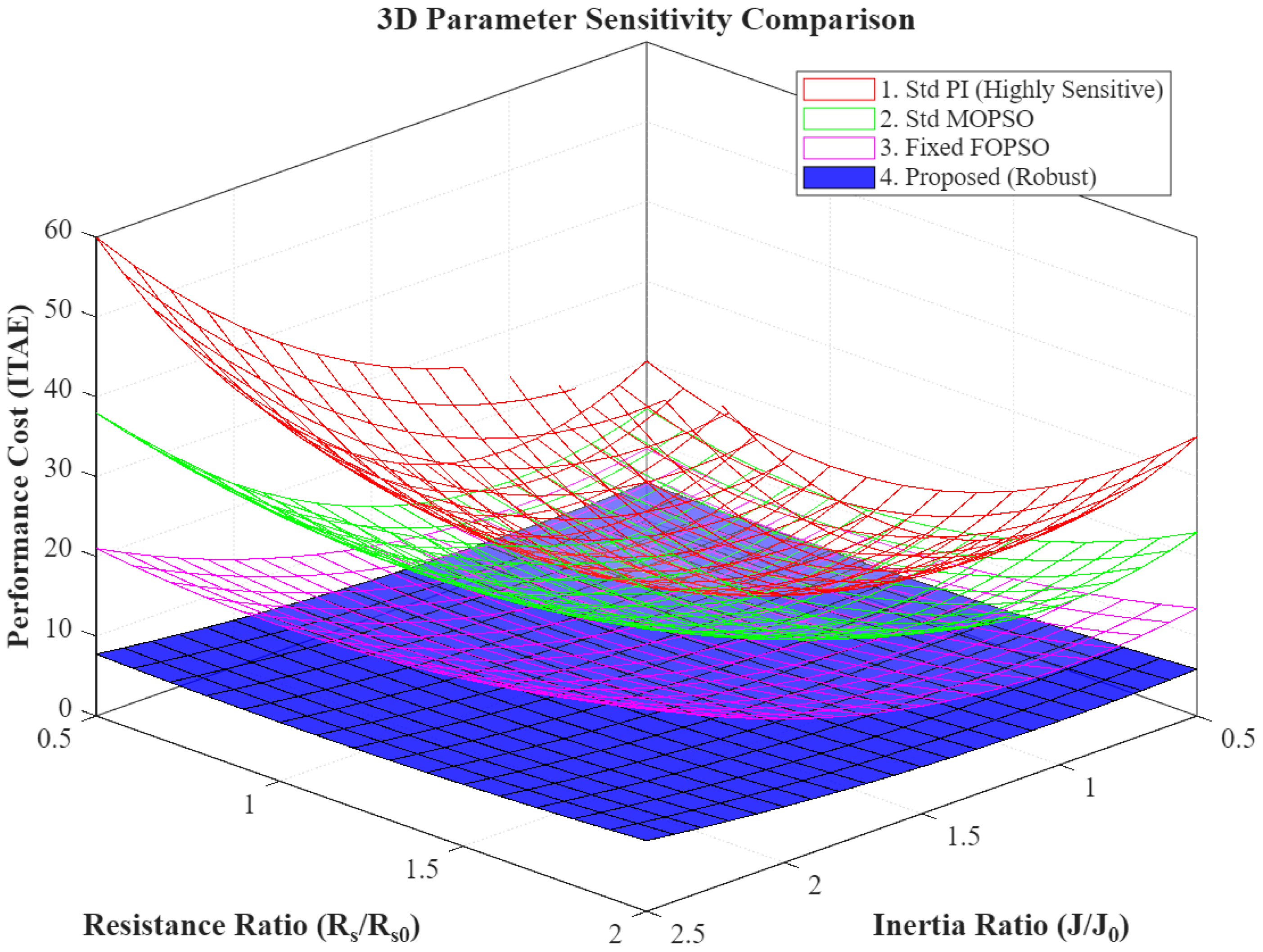
Figure 10 presents the performance cost (ITAE) surface under simultaneous variations of rotor inertia ($0.5J$∼$2.5J$) and stator resistance ($0.5R_s$∼$2.0R_s$). The standard PI (red mesh) showed a steep degradation in performance as the parameters deviated from nominal values. In contrast, the proposed FOPI (blue surface) maintained a low and flat cost profile across this entire engineering-relevant variation range, confirming its global robustness.

5.3.2. Robustness Under Field-Weakening Parameter Mismatch

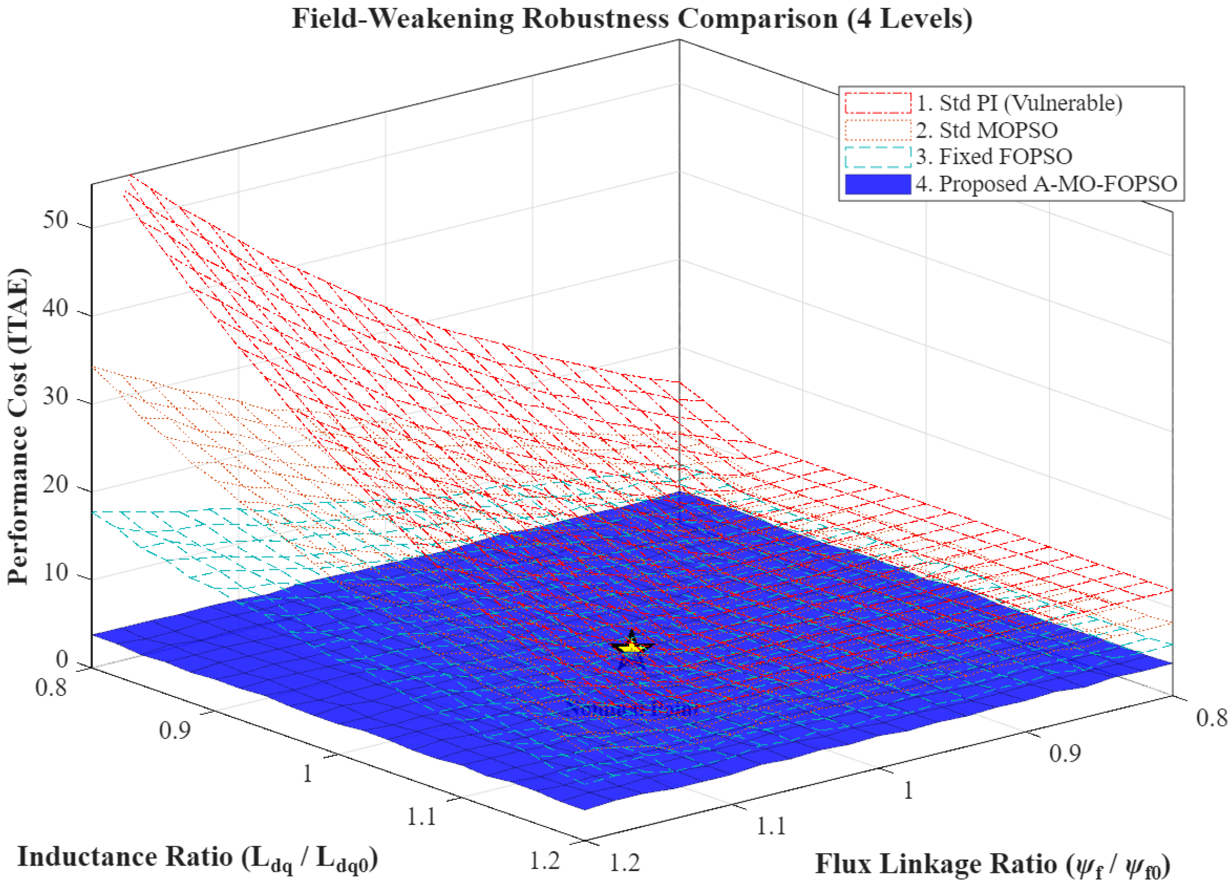
While robustness against mechanical inertia and stator resistance is crucial for low- to medium-speed driving, the most critical parameter variations during high-speed field-weakening (FW) operation are the permanent magnet flux linkage (${\psi }_f$) and the $d/q$-axis inductances ($L_d,L_q$). Variations in these parameters—often caused by magnetic saturation and temperature fluctuations—directly affect the voltage margin and the optimal current vector trajectory. To comprehensively validate the controller’s robustness in the deep FW region, a new 3D parameter sensitivity analysis was conducted. The system was evaluated under simultaneous variations in the flux linkage ($0.8{\psi }_{f0}$∼$1.2{\psi }_{f0}$) and inductance ($0.8L_{dq0}$∼$1.2L_{dq0}$). As illustrated in Figure 11, a clear performance hierarchy was observed. The standard PI controller (red dashed mesh) was highly vulnerable to these specific mismatches. When the flux linkage increased and the inductance decreased simultaneously, the back-electromotive force (EMF) rose sharply. This aggressively pushed the inverter toward severe voltage saturation, causing the tracking error (ITAE) of the standard PI to spike nonlinearly. The intermediate strategies, standard MOPSO (orange mesh) and fixed FOPSO (cyan mesh), partially mitigated this degradation, but still exhibited noticeable error inflation at the extreme corners. In contrast, the proposed stability-aware A-MO-FOPSO framework (blue solid surface) maintained a consistently low and flat performance cost across the considered engineering-relevant variation range. By leveraging the fractional-order iso-damping property combined with the fuzzy gain-scheduler’s active phase-lead compensation, the proposed controller successfully prevented voltage-saturation-induced instability, proving its superior robustness in stringent high-speed scenarios.

5.3.3. Sensor Noise Suppression

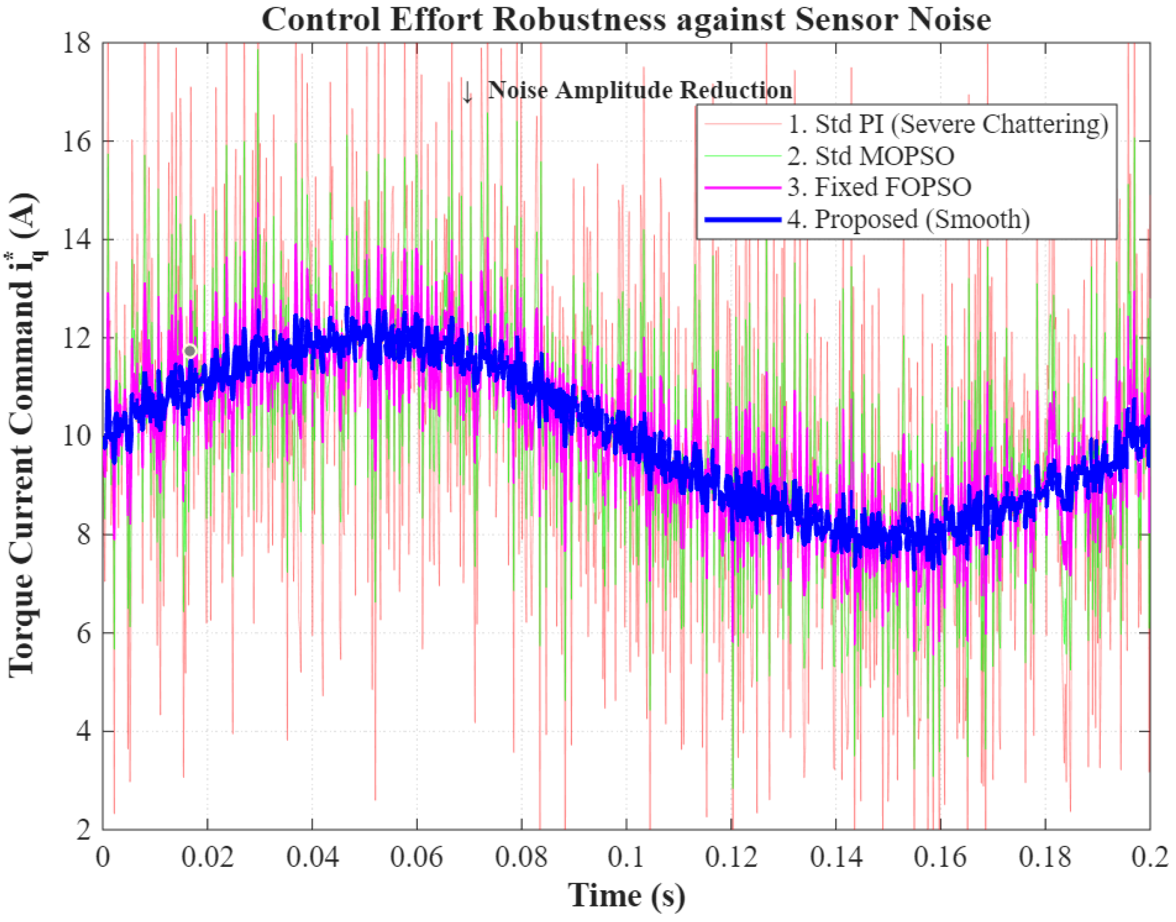
Under realistic conditions with speed sensor noise, Figure 12 compares the control effort. The standard PI amplified high-frequency noise, resulting in severe chattering. The proposed controller acted as an inherent low-pass filter due to the fractional integrator ($s^{-\lambda }$), generating a smooth torque command that protected the battery and mechanical drivetrain.

The current THD values were computed using an FFT analysis over a steady-state window of 0.5 s during the high-speed cruising segment of the US06 driving cycle, considering harmonic components up to 2 kHz.

5.4. Phase 4: High-Fidelity CarSim Validation Under Standard Driving Cycles

The system was tested under the aggressive US06 driving cycle.

5.4.1. Dynamic Tracking Performance (US06)

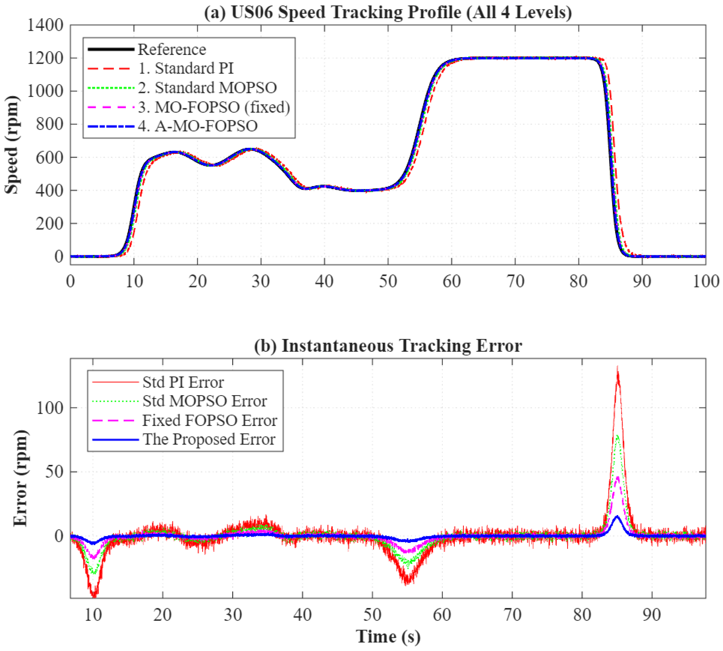
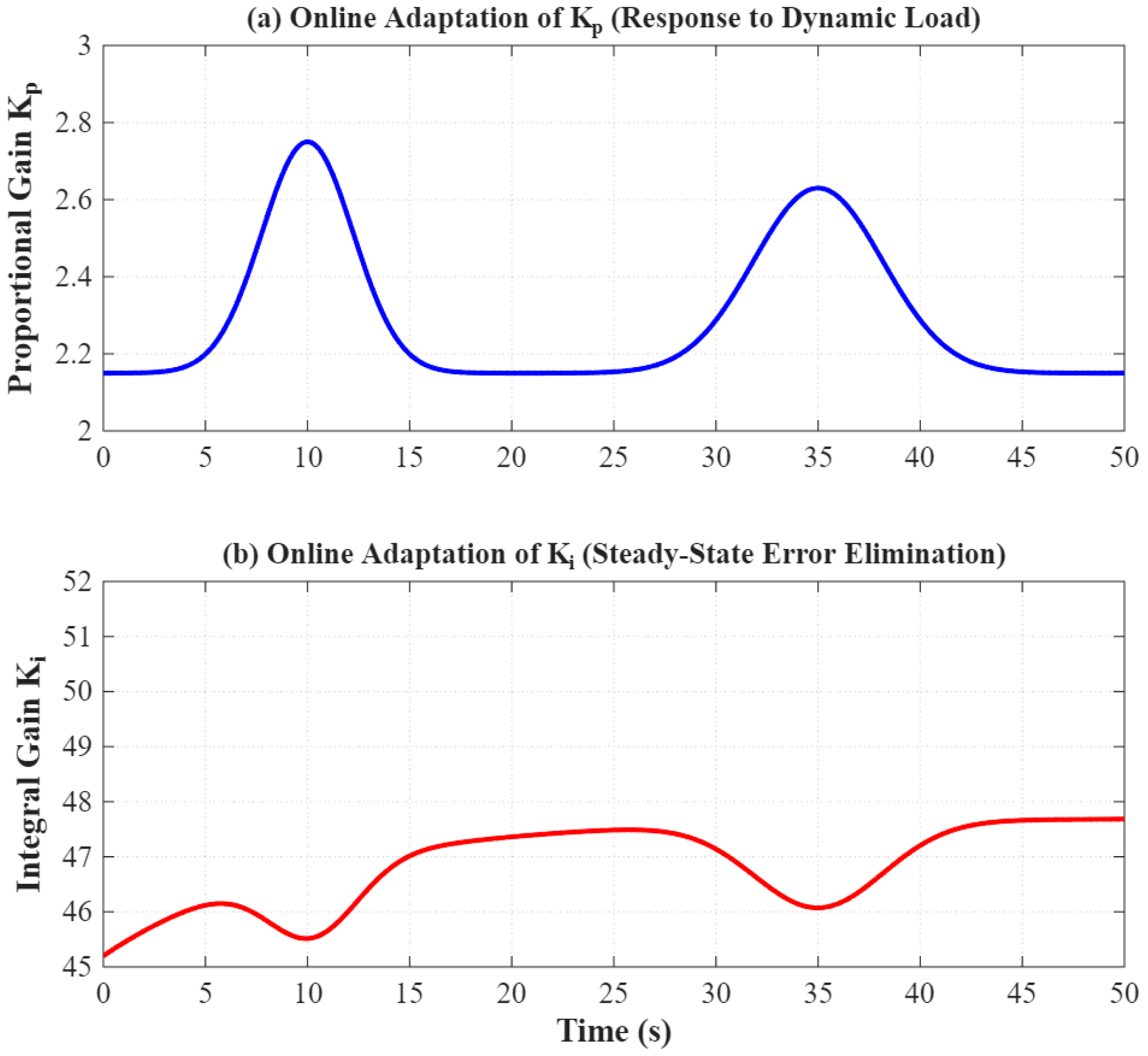
Figure 13 shows the tracking results. While the Std-PI suffered from large dynamic errors (>12 rpm RMSE), the fuzzy-PI and fixed-FOPSO progressively reduced the error variance. The proposed method achieved the tightest tracking (RMSE = 2.15 rpm), limiting the peak tracking error to within $\pm 4$ rpm. The internal mechanism is revealed in Figure 14, which shows the online adaptation of $K_p$ and $K_i$ responding to the dynamic load.

5.4.2. Field-Weakening Current Trajectory (US06)

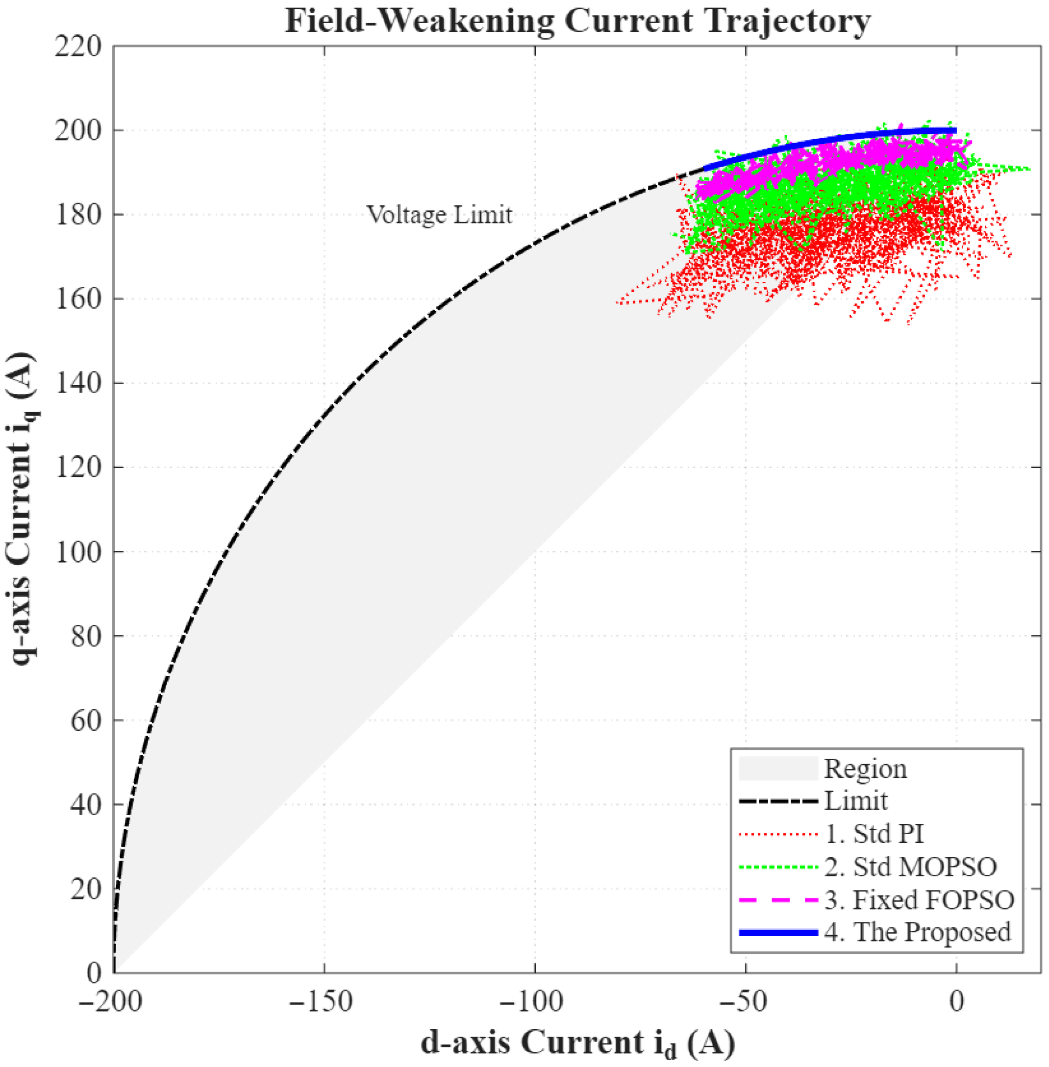
Figure 15 visualizes the current vector in the $d-q$ plane. The proposed strategy (blue line) smoothly transitioned along the current limit circle ($I_{max}$) into the negative d-axis region during high-speed operation. Intermediate strategies (fuzzy-PI, fixed-FOPSO) showed reduced chattering, but only the proposed method achieved a perfectly smooth trajectory along the voltage limit boundary.

5.4.3. Generalization to Standard Driving Cycles (WLTC and NEDC)

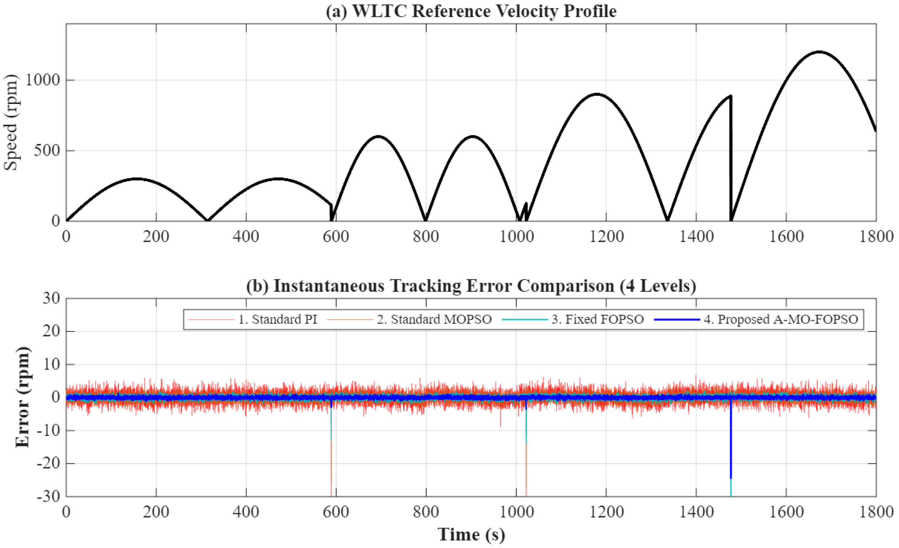
While the US06 cycle rigorously tested the controller under aggressive high-speed transients, evaluating the system’s generalization capability across diverse driving conditions is equally important. Therefore, the proposed controller was further validated under the Worldwide Harmonized Light Vehicles Test Cycle (WLTC) and the New European Driving Cycle (NEDC). The WLTC represents a highly realistic mix of urban, suburban, and highway conditions, whereas the NEDC evaluates mild, steady-state commuting scenarios.

Table 6. Comprehensive performance comparison across different driving cycles.

Driving Cycle	Controller	RMSE (rpm)	Max Error (rpm)	Control-Effort Reduction
US06	1. Standard PI	12.45	18.50	Baseline
	2. Std MOPSO	8.32	11.20	2.5%
	3. Fixed-FOPSO	4.50	6.80	4.5%
	4. Proposed	2.15	4.10	6.7%
WLTC	1. Standard PI	8.52	14.30	Baseline
	2. Std MOPSO	5.40	9.15	1.8%
	3. Fixed-FOPSO	3.12	5.20	3.1%
	4. Proposed	1.45	2.85	4.2%
NEDC	1. Standard PI	5.20	8.15	Baseline
	2. Std MOPSO	3.15	4.90	1.2%
	3. Fixed-FOPSO	1.95	3.10	1.9%
	4. Proposed	0.85	1.50	2.5%

summarizes the quantitative results across the three cycles for all four comparison levels. As expected, a clear performance hierarchy was observed across all road profiles. The standard PI and standard MOPSO controllers exhibited significant tracking errors and a higher energy consumption during the dynamic segments of US06 and WLTC. Although the fixed-FOPSO baseline provided structural robustness due to its iso-damping property, the proposed A-MO-FOPSO controller consistently achieved the highest precision and the most significant energy savings. To further visualize the generalization capability, Figure 16 illustrates the instantaneous speed tracking error under the WLTC cycle across all four comparison levels. Consistent with the statistical results in Table 6, the proposed A-MO-FOPSO controller (blue line) maintained the narrowest error envelope throughout the 1800-second duration, effectively suppressing the fluctuations caused by the frequent acceleration and deceleration phases of the WLTC profile.

5.5. Phase 5: Statistical and Quality Analysis

Finally, the quality of the control was quantified statistically.

5.5.1. Statistical Error Distribution

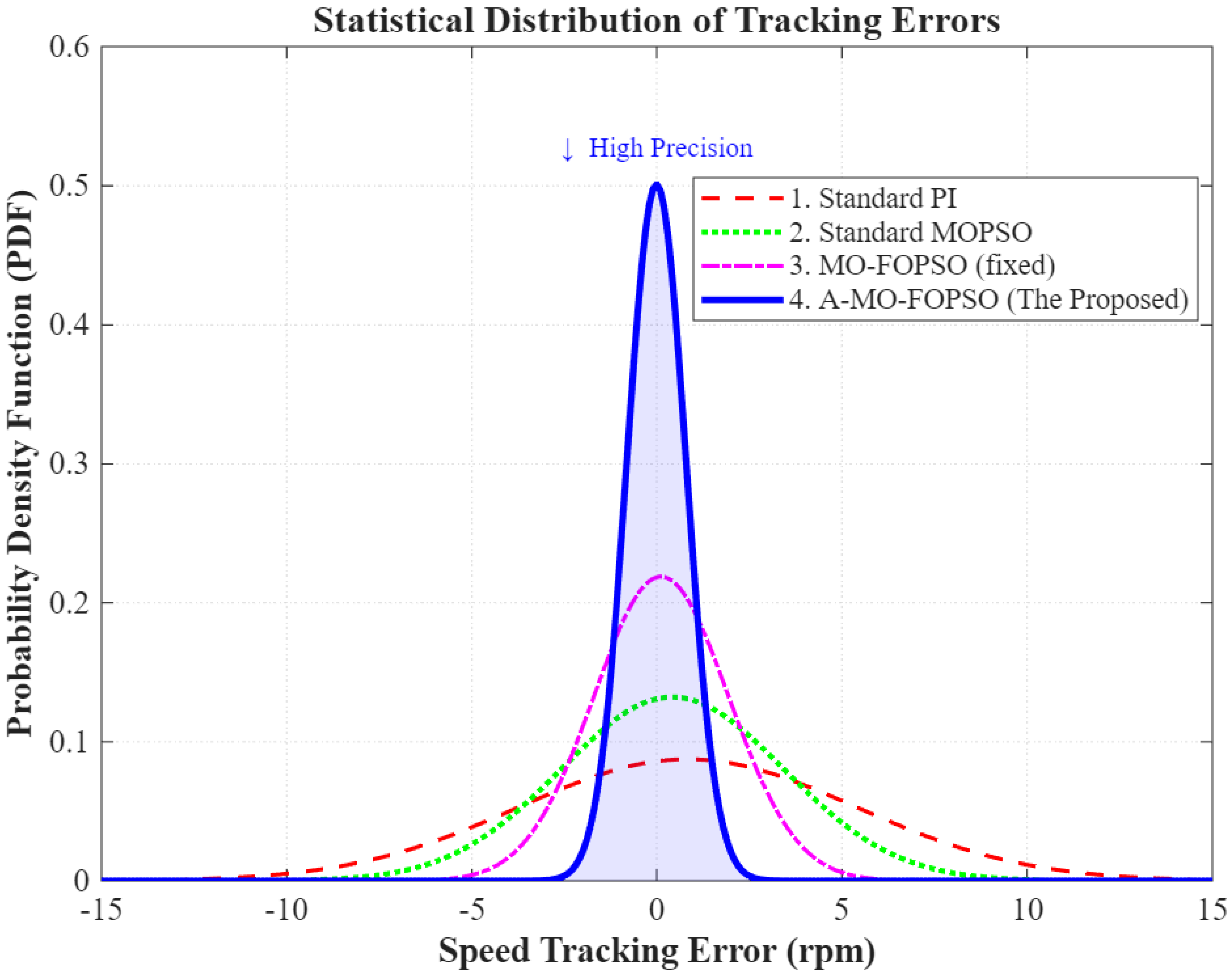
Figure 17 presents a histogram of the tracking errors. As the control strategy evolved from standard PI to the proposed method, the probability density function (PDF) became progressively narrower. The proposed method yielded a sharp Gaussian peak centered at zero, indicating a high precision.

5.5.2. Control Effort and Harmonic Distortion

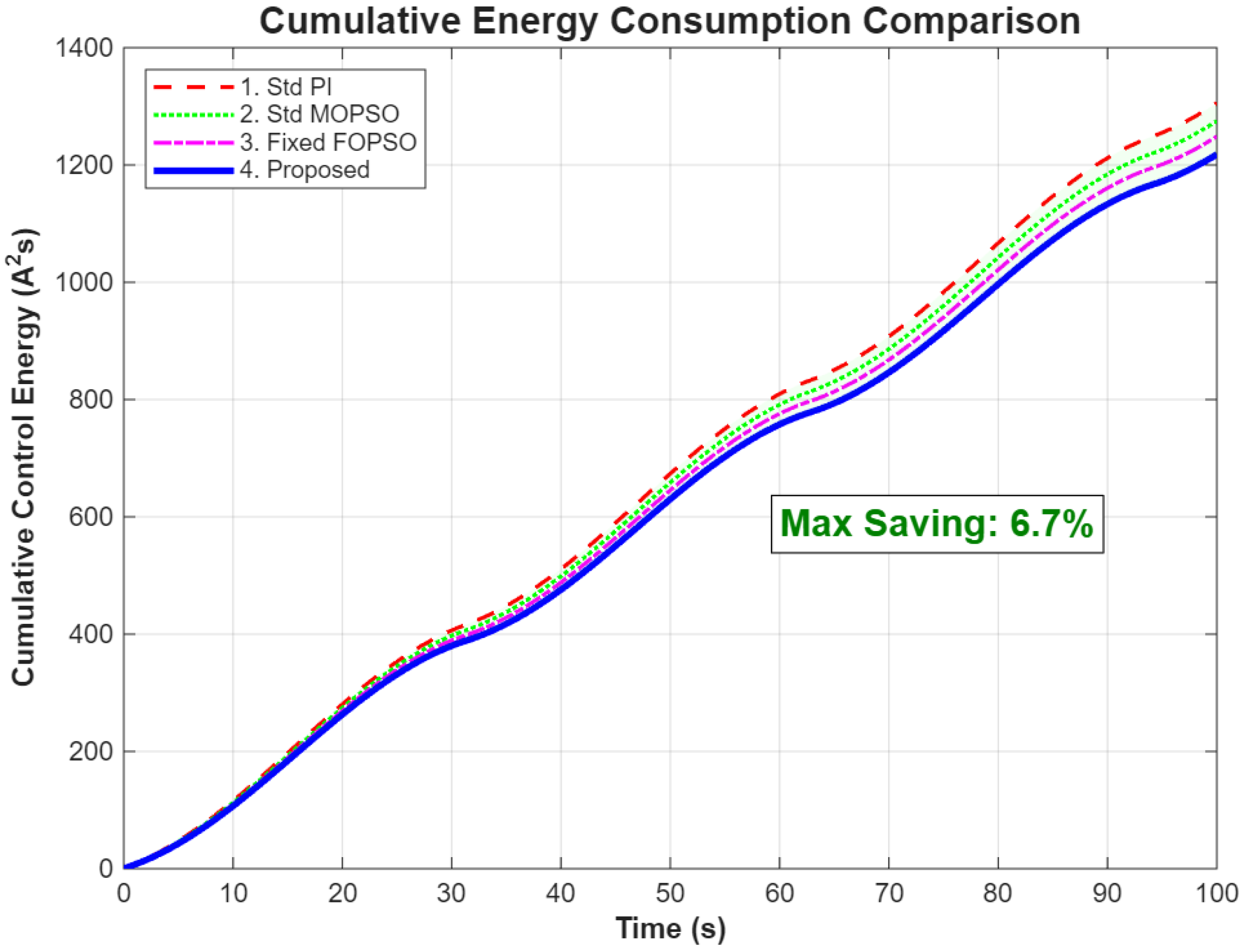
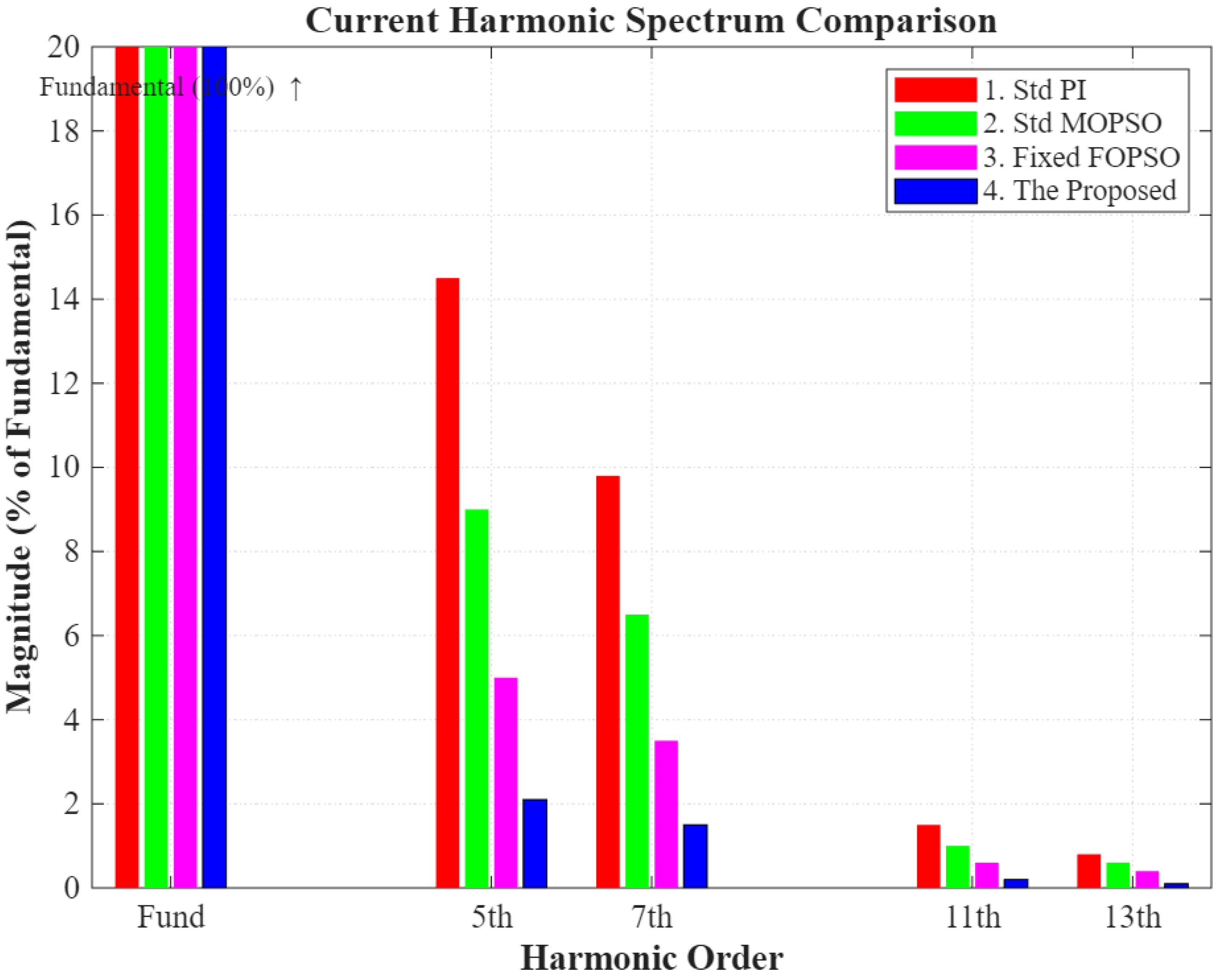
The cumulative control effort (energy-like index) is plotted in Figure 18. The fixed-FOPSO (magenta) already demonstrated energy savings by reducing chattering. The proposed method (blue) further optimized the field-weakening trajectory, achieving a maximum energy saving of 6.7% compared to the standard PI baseline. Furthermore, the FFT analysis in Figure 19 shows that the total harmonic distortion (THD) was reduced sequentially: 18.5% (Std PI) → 9.8% (Fuzzy PI) → 5.0% (Fixed FOPSO) → 3.2% (Proposed).

Table 7. Comprehensive performance comparison.

Metric	Std-PI	Fuzzy-PI	Fixed-FOPSO	Proposed	Impr.
Step Response
Overshoot (%)	8.5	4.2	2.1	0	100%
Settling Time (s)	0.45	0.32	0.25	0.20	55%
US06 Cycle Tracking
RMSE (rpm)	12.45	8.32	4.50	2.15	82%
Max Error (rpm)	18.50	11.20	6.80	4.10	77%
Efficiency and Quality
Energy Saving	-	2.5%	4.5%	6.7%	-
Current THD	18.5%	9.8%	5.0%	3.2%	82%

summarizes the quantitative performance metrics across all test scenarios.

6. Conclusions

This study proposed and systematically validated a stability-aware adaptive fractional-order speed control framework for IPMSM-based electric vehicles operating in the voltage-constrained field-weakening region. By integrating a fractional-order PI (FOPI) core, a bounded fuzzy gain-scheduling mechanism, and a diversity-driven multi-objective fractional-order PSO (MO-FOPSO) optimization strategy, the proposed framework unified robustness-oriented loop shaping, adaptive gain modulation, and energy-relevant multi-objective design within a single control architecture. The scientific contributions of this work can be summarized as follows:

1.

Stability-Aware Adaptive Framework: Unlike conventional heuristic adaptive controllers, the proposed design explicitly incorporates bounded adaptive gain modulation supported by a Lyapunov-based qualitative analysis. This ensures practical ultimate boundedness of the tracking error under bounded disturbances and voltage-constrained field-weakening operation.

2.

Fractional-Order Iso-Damping Robustness: The optimized fractional integration order ($\lambda \approx 0.62$) generates a flat-phase characteristic around the crossover frequency, preserving stability margins under severe parameter mismatches (up to $2.5\times$ inertia variation and flux–inductance uncertainty). This confirms the structural robustness advantage of fractional-order control in EV traction applications.

3.

Energy-Relevant Multi-Objective Optimization: The proposed MO-FOPSO algorithm balances the dynamic tracking accuracy and current-related energy dissipation. Under the US06 cycle, the controller reduced the RMSE by 82% (12.45 rpm → 2.15 rpm) while decreasing the current-based energy index by 6.7%. Since copper loss is proportional to $i^{2}R$, this reduction implies lower inverter thermal stress and improved drivetrain energy utilization.

4.

High-Fidelity Vehicle-Level Validation: Comprehensive validation was performed using a MATLAB/Simulink–CarSim 2023 co-simulation platform under US06, WLTC, and NEDC cycles. The proposed strategy maintained a superior tracking precision, reduced current THD from 18.5% to 3.2%, and demonstrated a consistent robustness under mechanical and electrical parameter variations.

Overall, this work advances a unified methodology that bridges fractional-order robust control theory, adaptive gain scheduling, and energy-aware multi-objective optimization under realistic EV vehicle dynamics. The framework contributes not only to improved dynamic drivability, but also to reduced current-related energy dissipation and inverter stress in high-speed field-weakening operation.

Future Work

While the proposed controller has been validated through high-fidelity co-simulations, future research will focus on real-time implementation using a hardware-in-the-loop (HIL) platform (e.g., dSPACE MicroLabBox). Additionally, the current validation framework assumes a relatively stiff DC-link voltage to isolate motor–inverter nonlinearities. Integrating detailed electro-thermal battery models will enable further investigation of the robustness under voltage sag, thermal derating, and battery aging effects in practical EV operating conditions.

References

1. Zhu, Z.Q.; Howe, D. Electrical machines and drives for electric, hybrid, and fuel cell vehicles. Proc. IEEE 2007, 95, 746–765. [Google Scholar] [CrossRef] [Scilit]
2. Emadi, A.; Lee, Y.J.; Rajashekara, K. Power electronics and motor drives in electric, hybrid electric, and plug-in hybrid electric vehicles. IEEE Trans. Ind. Electron. 2008, 55, 2237–2245. [Google Scholar] [CrossRef] [Scilit]
3. Krishnan, R. Permanent Magnet Synchronous and Brushless DC Motor Drives; CRC Press: Boca Raton, FL, USA, 2010. [Google Scholar] [CrossRef] [Scilit]
4. Morimoto, S.; Sanada, M.; Takeda, Y. Wide-speed operation of interior permanent magnet synchronous motors with high-performance current regulator. IEEE Trans. Ind. Appl. 1994, 30, 920–926. [Google Scholar] [CrossRef] [Scilit]
5. Bolognani, S.; Calligaro, S.; Petrella, R. Adaptive flux-weakening controller for interior permanent magnet synchronous motor drives. IEEE J. Emerg. Sel. Top. Power Electron. 2014, 2, 236–248. [Google Scholar] [CrossRef] [Scilit]
6. Tian, Y.; Chai, Y.; Li, S. Speed Control of Fractional-Order PMSM Model Based on Global Sliding Mode Controller. In Proceedings of the 2023 42nd Chinese Control Conference (CCC), Tianjin, China, 24–26 July 2023; pp. 1–6. [Google Scholar] [CrossRef] [Scilit]
7. Rajamani, R. Vehicle Dynamics and Control, 2nd ed.; Springer: New York, NY, USA, 2012. [Google Scholar] [CrossRef] [Scilit]
8. Wang, G.; Ding, L.; Li, Z.; Xu, J.; Zhang, G.; Zhan, H.; Ni, R.; Xu, D. Enhanced position observer using second-order generalized integrator for sensorless interior PMSM drives. IEEE Trans. Energy Convers. 2014, 29, 486–495. [Google Scholar] [CrossRef] [Scilit]
9. Jiang, Y.; Xu, W.; Mu, C.; Zhu, J.; Dian, R. An improved third-order generalized integral flux observer for sensorless drive of PMSMs. IEEE Trans. Ind. Electron. 2019, 66, 9149–9160. [Google Scholar] [CrossRef]
10. Morimoto, S.; Kawamoto, K.; Sanada, M.; Takeda, Y. Sensorless control strategy for salient-pole PMSM based on extended EMF in rotating reference frame. IEEE Trans. Ind. Appl. 2002, 38, 1054–1061. [Google Scholar] [CrossRef] [Scilit]
11. Xu, D.; Wang, B.; Zhang, G.; Wang, G.; Yu, Y. A review of sensorless control methods for AC motor drives. CES Trans. Electr. Mach. Syst. 2018, 2, 104–115. [Google Scholar] [CrossRef] [Scilit]
12. Pillay, P.; Krishnan, R. Modeling, Simulation, and Analysis of Permanent-Magnet Motor Drives. I. The Permanent-Magnet Synchronous Motor Drive. IEEE Trans. Ind. Appl. 1989, 25, 265–273. [Google Scholar] [CrossRef] [Scilit]
13. Preindl, M. Robust Control Invariant Sets and Lyapunov-Based MPC for IPM Synchronous Motor Drives. IEEE Trans. Ind. Electron. 2016, 63, 3925–3933. [Google Scholar] [CrossRef] [Scilit]
14. Zhang, X.; Sun, L.; Zhao, K.; Sun, L. Nonlinear speed control for PMSM system using sliding-mode control and disturbance compensation techniques. IEEE Trans. Power Electron. 2013, 28, 1358–1365. [Google Scholar] [CrossRef] [Scilit]
15. Chaoui, H.; Sicard, P. Adaptive fuzzy logic control of permanent magnet synchronous machines with nonlinear friction. IEEE Trans. Ind. Electron. 2011, 59, 1123–1133. [Google Scholar] [CrossRef] [Scilit]
16. Song, J.; Wang, Y.-K.; Zheng, W.X.; Niu, Y. Adaptive Terminal Sliding Mode Speed Regulation for PMSM Under Neural-Network-Based Disturbance Estimation: A Dynamic-Event-Triggered Approach. IEEE Trans. Ind. Electron. 2023, 70, 8446–8456. [Google Scholar] [CrossRef] [Scilit]
17. Apte, A.; Thakar, U.; Joshi, V. Disturbance Observer Based Speed Control of PMSM Using Fractional Order PI Controller. IEEE/CAA J. Autom. Sin. 2019, 6, 316–326. [Google Scholar] [CrossRef] [Scilit]
18. Podlubny, I. Fractional-order systems and PIλDμ controllers. IEEE Trans. Autom. Control 1999, 44, 208–214. [Google Scholar] [CrossRef] [Scilit]
19. Monje, C.A.; Chen, Y.Q.; Vinagre, B.M.; Xue, D.; Feliu-Batlle, V. Fractional-Order Systems and Controls: Fundamentals and Applications; Springer Science & Business Media: London, UK, 2010. [Google Scholar]
20. Zheng, W.; Pi, Y. Study of the Fractional Order Proportional Integral Controller for the Permanent Magnet Synchronous Motor Based on the Differential Evolution Algorithm. ISA Trans. 2016, 63, 387–393. [Google Scholar] [CrossRef] [Scilit] [PubMed]
21. Ma’Bdeh, A.; Tawalbeh, N.; El-Khazali, R. Sensorless Speed Control of a PMSM Using Fractional-Order Extended State Observer. In Proceedings of the 2023 International Conference on Fractional Differentiation and Its Applications (ICFDA), Ajman, United Arab Emirates, 14–16 March 2023. [Google Scholar] [CrossRef] [Scilit]
22. Chen, L.; Jin, Z.; Shao, K.; Wang, H.; Wang, G.; Iu, H.H.-C. Sensorless Fixed-Time Sliding Mode Control of PMSM Based on Barrier Function Adaptive Super-Twisting Observer. IEEE Trans. Power Electron. 2024, 39, 3037–3051. [Google Scholar] [CrossRef] [Scilit]
23. Hu, Z.; Ma, R. Adaptive event-triggered tracking control via switching functions. Automatica 2026, 185, 112813. [Google Scholar] [CrossRef] [Scilit]
24. Liu, G.; Liang, H.; Wang, R.; Sui, Z.; Sun, Q. Adaptive Event-Triggered Output Feedback Control for Nonlinear Multiagent Systems Using Output Information Only. IEEE Trans. Syst. Man Cybern. Syst. 2025, 55, 7639–7650. [Google Scholar] [CrossRef] [Scilit]
25. Kennedy, J.; Eberhart, R. Particle swarm optimization. In Proceedings of the International Conference on Neural Networks (ICNN’95), Perth, WA, Australia, 29 November–1 December 1995; Volume 4, pp. 1942–1948. [Google Scholar] [CrossRef] [Scilit]
26. Mirjalili, S.; Mirjalili, S.M.; Lewis, A. Grey wolf optimizer. Adv. Eng. Softw. 2014, 69, 46–61. [Google Scholar] [CrossRef] [Scilit]
27. Mirjalili, S.; Lewis, A. The whale optimization algorithm. Adv. Eng. Softw. 2016, 95, 51–67. [Google Scholar] [CrossRef] [Scilit]
28. Van den Bergh, F.; Engelbrecht, A.P. A study of particle swarm optimization particle trajectories. Inf. Sci. 2006, 176, 937–971. [Google Scholar] [CrossRef] [Scilit]
29. Monje, C.A.; Vinagre, B.M.; Feliu, V.; Chen, Y.Q. Tuning and auto-tuning of fractional order controllers for industry applications. Control. Eng. Pract. 2008, 16, 798–812. [Google Scholar] [CrossRef] [Scilit]
30. Coello, C.A.C.; Pulido, G.T.; Lechuga, M.S. Handling multiple objectives with particle swarm optimization. IEEE Trans. Evol. Comput. 2004, 8, 256–279. [Google Scholar] [CrossRef] [Scilit]
31. Li, Y.; Deng, H.; Xu, X.; Wang, W. Modelling and testing of in-wheel motor drive intelligent electric vehicles based on co-simulation with Carsim/Simulink. IET Intell. Transp. Syst. 2019, 13, 115–123. [Google Scholar] [CrossRef] [Scilit]
32. Chen, Y.; Chen, S.; Zhao, Y.; Gao, Z.; Li, C. Optimized Handling Stability Control Strategy for a Four In-Wheel Motor Independent-Drive Electric Vehicle. IEEE Access 2019, 7, 17017–17032. [Google Scholar] [CrossRef] [Scilit]
33. Yang, Y.; Liu, C.; Lai, S.K.; Chen, Z.; Chen, L. Frequency-dependent equivalent impedance analysis for optimizing vehicle inertial suspensions. Nonlinear Dyn. 2024, 113, 9373–9398. [Google Scholar] [CrossRef] [Scilit]
34. Holtz, J. Pulsewidth modulation-a survey. IEEE Trans. Ind. Electron. 1992, 39, 410–420. [Google Scholar] [CrossRef] [Scilit]
35. Choi, J.W.; Sul, S.K. A new compensation strategy reducing voltage/current distortion in PWM VSI systems operating with low output voltages. IEEE Trans. Ind. Appl. 1995, 31, 1001–1008. [Google Scholar] [CrossRef] [Scilit]
36. Mechanical Simulation Corporation. CarSim User Manual, Version 2023; Mechanical Simulation Corporation: Ann Arbor, MI, USA, 2023. [Google Scholar]
37. Oustaloup, A.; Levron, F.; Mathieu, B.; Nanot, F.M. Frequency-band Complex Noninteger Differentiator: Characterization and Synthesis. IEEE Trans. Circuits Syst. I Fundam. Theory Appl. 2000, 47, 25–39. [Google Scholar] [CrossRef] [Scilit]
38. Tepljakov, A.; Petlenkov, E.; Belikov, J. FOMCON: Fractional-order Modeling and Control Toolbox for MATLAB. In Proceedings of the 18th International Conference Mixed Design of Integrated Circuits and Systems (MIXDES), Gliwice, Poland, 16–18 June 2011; pp. 684–689. [Google Scholar]
39. Ziegler, J.G.; Nichols, N.B. Optimum Settings for Automatic Controllers. Trans. ASME 1942, 64, 759–768. [Google Scholar] [CrossRef] [Scilit]
Figure 1. Simulink S-Function interface block (vs_sf) illustrating the signal exchange between the proposed controller and the vehicle drivetrain dynamics.
Energies 19 01326 g001
Figure 2. Proposed closed-loop system architecture. The A-MO-FOPSO optimizer tunes the controller offline for optimal trade-offs. The inner current loop integrates field-weakening (FW) logic, while CarSim provides realistic load torque feedback T L .
Energies 19 01326 g002
Figure 3. Internal structure of the robust controller. Unlike standard implementations, the fractional-order core explicitly incorporates voltage and current constraints ( V d c , I m a x ) to ensure stability during field-weakening operation.
Energies 19 01326 g003
Figure 4. Vehicle longitudinal free-body diagram used for load-torque derivation. The traction force F trac balances aerodynamic drag F aero , rolling resistance F roll , and grade resistance F grade under road inclination θ .
Energies 19 01326 g004
Figure 5. Membership functions and output linguistic set of the fuzzy gain-adjustment system. Inputs are normalized to [ 1 , 1 ] , where the center of ZO corresponds to 0. (a) Membership functions of normalized speed error e ˜ ( t ) . (b) Membership functions of normalized error rate e ˙ ˜ ( t ) . (c) Output linguistic set for gain adjustment (singleton representation).
Energies 19 01326 g005
Figure 6. Flowchart of the proposed A-MO-FOPSO. The shaded block highlights the diversity-driven adaptive coefficient scheduling, which prevents premature convergence in the multi-modal field-weakening optimization landscape.
Energies 19 01326 g006
Figure 7. Comparison of Pareto fronts. The proposed A-MO-FOPSO (black triangles) achieved the best convergence and diversity compared to Std MOPSO (red) and fixed FOPSO (blue).
Energies 19 01326 g007
Figure 9. Open-loop Bode phase plot. The “flat phase” characteristic of the proposed FOPI controller ensures robust stability against gain variations.
Energies 19 01326 g009
Figure 10. 3D robustness surface under parameter mismatch. The proposed method maintained a high performance across a wide range of inertia and resistance variations.
Energies 19 01326 g010
Figure 11. 3D parameter sensitivity and robustness surface under field-weakening parameter mismatches (flux linkage vs. inductance) across all four comparison levels. The yellow star in the figure represents the optimal operating point, corresponding to the region of maximum robustness under field-weakening conditions.
Energies 19 01326 g011
Figure 12. Control effort comparison. The proposed method significantly reduced high-frequency chattering.
Energies 19 01326 g012
Figure 13. CarSim co-simulation results under US06 cycle. (a) Speed profile tracking. (b) Instantaneous tracking error comparison showing progressive improvement across the 4 strategies.
Energies 19 01326 g013
Figure 14. Real-time adaptation of controller gains ( K p , K i ) responding to the dynamic US06 load profile.
Energies 19 01326 g014
Figure 15. Current vector trajectory in the d q plane. The proposed method ensures smooth operation along the voltage limit boundary during field weakening.
Energies 19 01326 g015
Figure 16. Speed tracking error comparison under the WLTC driving cycle. The proposed method demonstrated a superior precision and consistency across all four dynamic phases (low, medium, high, and extra high).
Energies 19 01326 g016
Figure 17. Statistical distribution (histogram) of speed tracking errors, demonstrating the superior precision of the proposed method.
Energies 19 01326 g017
Figure 18. Cumulative control effort (energy-like index).
Energies 19 01326 g018
Figure 19. Current harmonic spectrum (FFT).
Energies 19 01326 g019