Finite Element Simulation and Experimental Study of a Redesigned Solar Thermal Prototype with Parabolic Concentration

Abstract

This study proposes a novel redesign of a solar water heater prototype by integrating a stationary compound parabolic concentrator (CPC) internally within a standard collector housing. Unlike conventional flat-plate systems or external trough collectors, this design aims to enhance thermal efficiency while maintaining a compact footprint suitable for residential retrofitting in tropical climates. The system’s thermal performance was analyzed using a 3D finite element method (FEM) based on the convection-diffusion equation, with a specific focus on a 2 cm focal length configuration designed to fit spatial constraints. The simulation results indicated a maximum water temperature of 62.9 °C under concentrated solar flux, while the experimental prototype achieved a maximum temperature of 55.0 °C under corresponding field conditions. The comparative analysis reveals a temperature discrepancy of approximately 8 °C (12.5%), which is attributed to the simplified boundary conditions neglecting radiative losses in the model. Despite this deviation, the proposed parabolic design demonstrated a distinct thermal enhancement compared to the conventional baseline. These findings validate the technical feasibility of the compact internal concentrator, offering a low-cost, high-performance alternative for domestic water heating applications.

1. Introduction

Solar energy is widely recognized as one of the most abundant and sustainable renewable resources. Specifically, the thermal component of solar radiation offers significant potential for practical applications, particularly for water heating in residential and commercial sectors, such as hotels. Despite Thailand’s high solar potential, the hospitality and residential sectors continue to rely heavily on conventional electric water heaters, leading to substantial energy inefficiencies and increased costs. Consequently, the advancement of solar thermal technology is essential as a strategic solution to reduce energy consumption, lower greenhouse gas emissions, and promote long-term sustainability in tropical regions.

To enhance system performance, recent advancements in solar thermal technology have increasingly relied on computational methods. The literature highlights the critical role of numerical simulation in optimizing concentrating solar collectors. For instance, computational modeling has been utilized to assess the thermal performance of parabolic trough collectors (PTCs), emphasizing the impact of receiver tube geometry on temperature uniformity [1]. Furthermore, the application of three-dimensional (3D) numerical analysis has proven effective in predicting complex temperature fields in solar receivers, as demonstrated by research that integrated fluid-thermal coupling to validate system designs [2]. Additionally, recent work employed FEM specifically to analyze the thermal yield of hybrid parabolic concentrator systems, confirming that FEM is a robust tool for accurately simulating heat transfer phenomena in complex geometries [3]. Validating these numerical models with experimental data remains a cornerstone of reliable research, as seen in investigations that coupled simulation with thermal imaging to verify efficiency improvements in novel collector designs [4].

Regarding the choice of numerical method, while differential equations describe the majority of engineering problems, they are often challenging to solve analytically. Although FDM is straightforward to implement, it has limitations in specifying boundary conditions for complex structures. In contrast, FEM helps address these issues by accurately representing the original shape in a detailed and realistic manner [5]. This capability is particularly vital for designing the curved surfaces of parabolic concentrators.

The recent literature from 2023 to 2024 has extensively explored methods to further enhance the efficiency of PTCs. For instance, Limboonruang et al. (2023) [6] demonstrated that modifying receiver geometries with external fins significantly improves heat transfer. Furthermore, Mahdhi et al. (2025) [7] investigated stationary PTCs specifically for domestic water heating, highlighting the potential of simplified tracking systems. Recent studies in 2021–2024 have further explored advanced techniques to maximize collector efficiency. For example, research published in Elsevier investigated the use of nanofluids and twisted tape inserts to enhance the thermal conductivity of parabolic trough collectors [8]. While these methods successfully increase heat transfer rates, they often introduce higher hydraulic resistance and operational costs. Similarly, a study in Elsevier focused on the techno-economic optimization of solar water heaters for residential buildings, highlighting the importance of system integration [9]. Furthermore, recent numerical investigations in Appl. Sci have analyzed complex geometric modifications to the receiver tube to improve optical efficiency [10]. However, most existing studies focus on large-scale power generation or require complex external layouts. There remains a significant research gap regarding compact, internal parabolic concentrators integrated directly into household water heaters for tropical climates that are both cost-effective and easy to fabricate.

Therefore, the novelty of this study lies in the development of a compact, static parabolic solar water heater design that bridges this gap. Unlike previous works that rely on complex tracking or 1D approximations, this research utilizes a simplified 3D FEM approach to evaluate the thermal gradients and validates the redesign with experimental prototyping. This study aims to provide a verified, efficient solution that balances thermal performance with the practical constraints of residential application.

It should be emphasized that numerical modeling in this study is positioned as a constrained-design, preliminary engineering validation rather than a high-precision multiphysics analysis. The objective is to practically assess the macroscopic thermal trends and structural feasibility of the parabolic concentrator prior to full-scale deployment.

This paper presents a mathematical model for predicting temperature distributions in solar thermal systems, governed by second-order partial differential equations. The contents are divided into six sections. Section 1 is an introduction. Section 2 describes materials and methods. Section 3 describes result of solar thermal. Section 4 presents designs of solar thermal prototype for experiment results. Section 5 presents comparison of simulation results and discussion. Lastly, a conclusion is in Section 6.

2. Materials and Methods

2.1. Thermal Analysis of Solar Thermal

PDE in Equation (1) shows 3D heat transfer equation with the heat source is used to obtain the temperature distribution in solar thermal [11].

$$k{\displaystyle \frac{\partial }{\partial x}}{\displaystyle \frac{\partial T}{\partial x}}+k{\displaystyle \frac{\partial }{\partial y}}{\displaystyle \frac{\partial T}{\partial y}}+k{\displaystyle \frac{\partial }{\partial z}}{\displaystyle \frac{\partial T}{\partial z}}-\rho c\left(u{\displaystyle \frac{\partial T}{\partial x}}+v{\displaystyle \frac{\partial T}{\partial y}}+w{\displaystyle \frac{\partial T}{\partial z}}\right)+Q=\rho c{\displaystyle \frac{\partial T}{\partial t}},$$

(1)

where k is thermal conductivity (W/m·°C), T is temperature (°C), ρ is the density of the mass (kg/m³), c is the capacity of the specific heat (J/kg·°C), Q is internal heat generation (W/m³), and u, v, and w is axis velocity of water flow x, y, and z, respectively (m/s).

2.2. Discretization

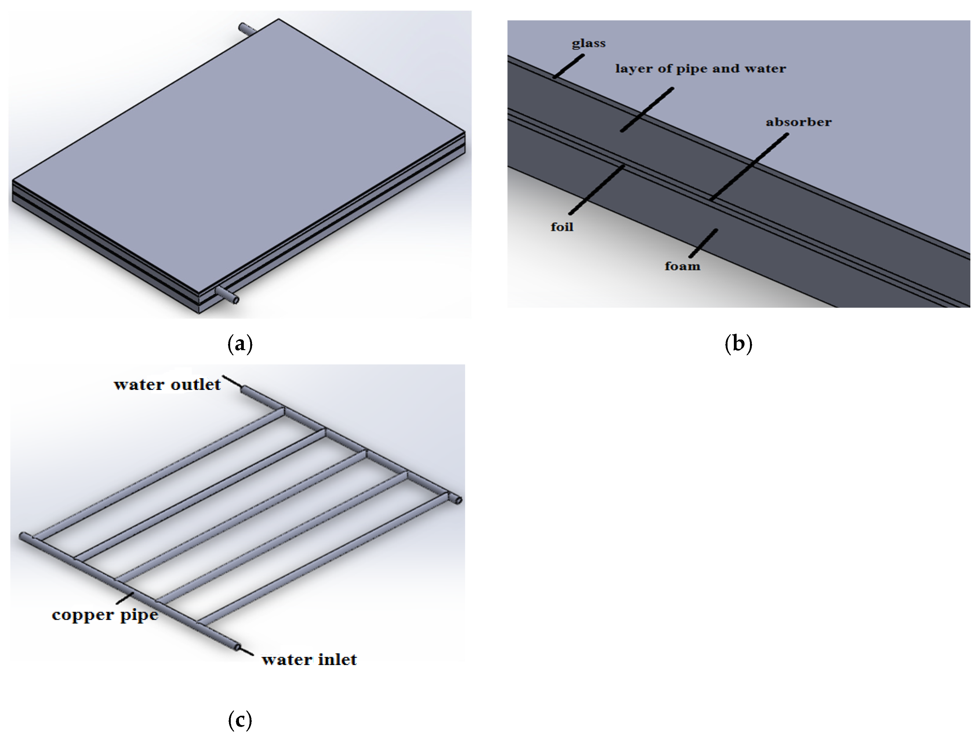
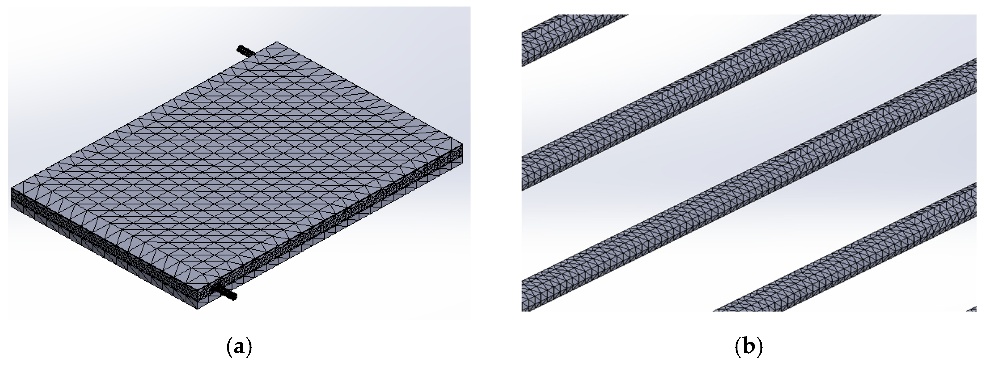
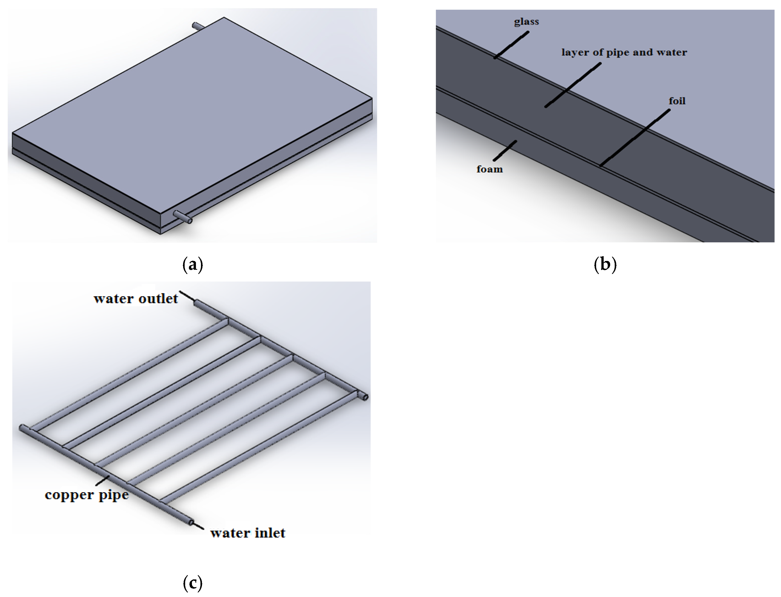
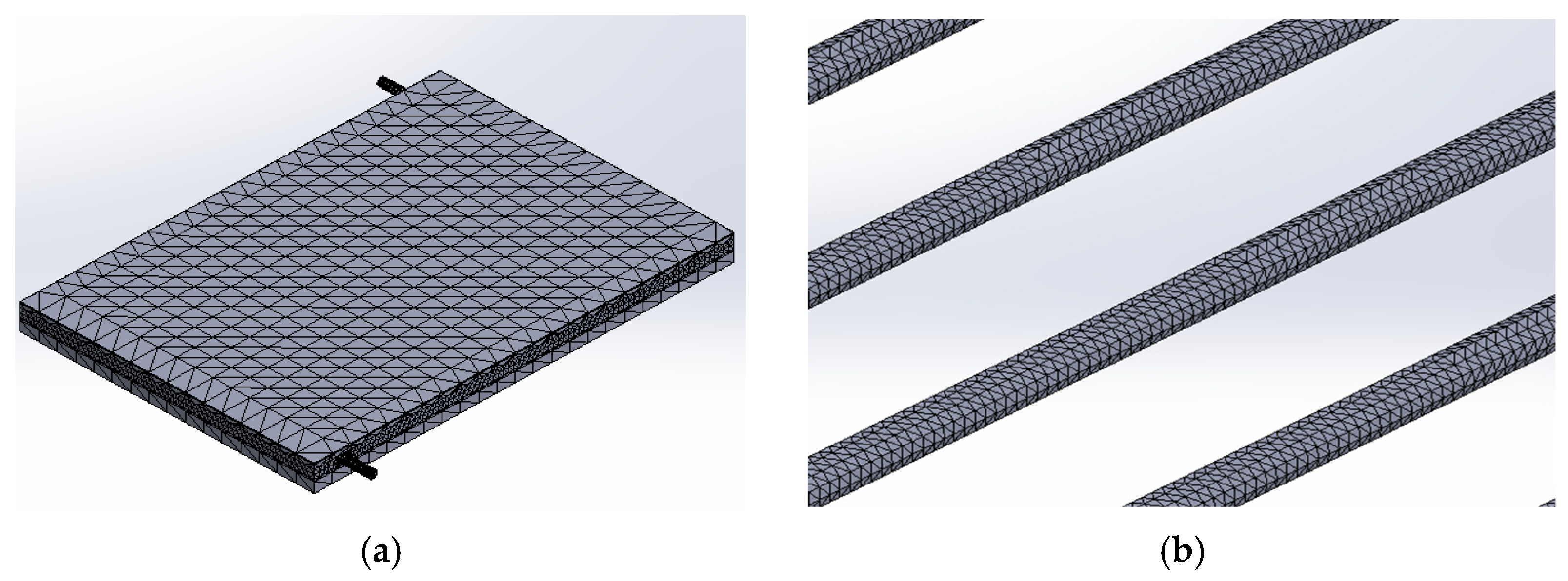
The domain of study can be discretized using linear tetrahedron elements when using the 3D FEM. Solid Work (Version 2024) for the production of 3D grids can achieve this property. Figure 1 depicts the specifics of a conventional solar thermal system with an absorber, whereas Figure 2 depicts the mesh of a conventional solar thermal system with an absorber. The mesh of pipe and water comprises 266,569 elements and 47,329 nodes. Figure 3 depicts specifics of the new solar thermal design with parabolic concentration and Figure 4 depicts a mesh of the new solar thermal design with parabolic concentration and pipe and water mesh with 119,035 nodes and 119,035 elements. The domain was discretized using linear tetrahedral elements. This element type was specifically chosen over hexahedral elements due to its superior adaptability to the complex curved geometries present in the system, specifically the parabolic reflector surface and the cylindrical receiver tube. Tetrahedral meshing avoids the element distortion often encountered when mapping hexahedral grids onto non-orthogonal curvatures, ensuring geometric fidelity and numerical stability. To conduct this preliminary engineering validation, the 3D-FEM model was established under specific constrained-design parameters. Deliberate physical simplifications were applied to balance computational efficiency with practical engineering assessment, avoiding the complexities of high-precision multiphysics solvers.

2.3. Formulation

In this study, the Galerkin weighted residual method was employed to ensure that each term in the governing heat-transfer equation satisfies the weighted integral formulation. A four-node tetrahedral element (linear 3-dimensional element) was adopted as the interpolation, or shape function, for approximating the temperature field within the finite element domain. Accordingly, the temperature distribution is expressed following the formulations presented in Equations (2) and (3), consistent with standard FEM heat-transfer analysis methods [12].

$$T\left(x,y,z\right)=T_1{N}_1+T_2{N}_2+T_3{N}_3+T_4{N}_4,$$

(2)

where N_i, i = 1, 2, 3, 4 is the element shape function, and the T_i, i = 1, 2, 3, 4 is the temperature of each node (1, 2, 3, 4, respectively) of the elements, then

$$N_i={\displaystyle \frac{1}{6V}}\left(a_i+b_{i}x+c_{i}y+d_{i}z\right),$$

(3)

where V is the volume of each element, which derived from Equation (4).

$$V={\displaystyle \frac{1}{6}}\left|\begin{array}{cccc}1& x_1& y_1& z_1\\ 1& x_2& y_2& z_2\\ 1& x_3& y_3& z_3\\ 1& x_4& y_4& z_4\end{array}\right|,$$

(4)

where

$$\begin{gathered} a_1=x_4(y_2{z}_3-y_3{z}_2)+x_3(y_4{z}_2-y_2{z}_4)+x_2(y_3{z}_4-y_4{z}_3) \\ {a}_2=x_4(y_3{z}_1-y_1{z}_3)+x_3(y_1{z}_4-y_4{z}_1)+x_1(y_4{z}_3-y_3{z}_4) \\ {a}_3=x_4(y_1{z}_2-y_2{z}_1)+x_2(y_4{z}_1-y_1{z}_4)+x_1(y_2{z}_4-y_4{z}_2) \\ {a}_4=x_3(y_2{z}_1-y_1{z}_2)+x_2(y_1{z}_3-y_3{z}_1)+x_1(y_3{z}_2-y_2{z}_3) \\ {b}_1=y_4(z_3-z_2)+y_3(z_2-z_4)+y_2(z_4-z_3) \\ {b}_2=y_4(z_3-z_2)+y_1(z_3-z_4)+y_3(z_4-z_1) \\ {b}_3=y_4(z_3-z_2)+y_2(z_1-z_4)+y_1(z_4-z_2) \\ {b}_4=y_3(z_3-z_2)+y_1(z_2-z_3)+y_2(z_3-z_1) \\ {c}_1=x_4(z_2-z_3)+x_2(z_3-z_4)+x_3(z_4-z_2) \\ {c}_2=x_4(z_3-z_1)+x_3(z_1-z_4)+x_1(z_4-z_3) \\ {c}_3=x_4(z_1-z_2)+x_1(z_2-z_4)+x_2(z_4-z_1) \\ {c}_4=x_3(z_2-z_1)+x_2(z_1-z_3)+x_1(z_3-z_2) \\ {d}_1=x_4(y_3-y_2)+x_3(y_2-y_4)+x_2(y_4-y_3) \\ {d}_2=x_4(y_1-y_3)+x_1(y_3-y_4)+x_3(y_4-y_1) \\ {d}_3=x_4(y_2-y_1)+x_2(y_1-y_4)+x_1(y_4-y_2) \\ {d}_4=x_3(y_1-y_2)+x_1(y_2-y_3)+x_2(y_3-y_1) \end{gathered}$$

From Equation (1) there is a Galerkin approach equation as referring to the differential equation; it was then adapted by using the weighted residual method, which element domain V as in Equation (4) was done by using the integrations as follow Equation (5) [13].

$${\int }_V{N}_n\rho c{\displaystyle \frac{\partial T}{\partial t}}dV+{\int }_{V}k\left({\displaystyle \frac{\partial N_n}{\partial x}}{\displaystyle \frac{\partial T}{\partial x}}+{\displaystyle \frac{\partial N_n}{\partial y}}{\displaystyle \frac{\partial T}{\partial y}}+{\displaystyle \frac{\partial N_n}{\partial z}}{\displaystyle \frac{\partial T}{\partial z}}\right)dV+{\int }_V{N}_n\rho c\left(u{\displaystyle \frac{\partial T}{\partial x}}+v{\displaystyle \frac{\partial T}{\partial y}}+w{\displaystyle \frac{\partial T}{\partial z}}\right)dV+{\int }_{\mathrm{\Gamma }}{N}_n\left(hT\right)d\mathrm{\Gamma }={\int }_V{N}_{n}QdV+{\int }_{\mathrm{\Gamma }}{N}_n\left(h{T}_{\mathrm{\infty }}\right)d\mathrm{\Gamma },$$

(5)

In the compact matrix form,

$${\left[C\right]}_{4\times 4}{\left\{\dot{T}\right\}}_{4\times 1}+{\left[\left[K_c\right]+\left[K_v\right]+\left[K_h\right]\right]}_{4\times 4}{\left\{T\right\}}_{4\times 1}={\left\{Q_Q\right\}}_{4\times 1}+{\left\{Q_h\right\}}_{4\times 1}.$$

(6)

$${\left[C\right]}_{4\times 4}={\displaystyle \frac{\rho cV}{20}}\left[\begin{array}{cccc}2& 1& 1& 1\\ 1& 2& 1& 1\\ 1& 1& 2& 1\\ 1& 1& 1& 2\end{array}\right].$$

(7)

$${\left[K_c\right]}_{4\times 4}={\displaystyle \frac{k}{36V}}\left[\begin{array}{cccc}{b}_1{b}_1+c_1{c}_1+d_1{d}_1& b_1{b}_2+c_1{c}_2+d_1{d}_2& b_1{b}_3+c_1{c}_3+d_1{d}_3& b_1{b}_4+c_1{c}_4+d_1{d}_4\\ -& b_2{b}_2+c_2{c}_2+d_2{d}_2& b_2{b}_3+c_2{c}_3+d_2{d}_3& b_2{b}_4+c_2{c}_4+d_2{d}_4\\ -& -& b_3{b}_3+c_3{c}_3+d_3{d}_3& b_3{b}_4+c_3{c}_4+d_3{d}_4\\ Sym& -& -& b_4{b}_4+c_4{c}_4+d_4{d}_4\end{array}\right].$$

(8)

$${\left[K_h\right]}_{4\times 4}={\displaystyle \frac{hV}{20}}\left[\begin{array}{cccc}2& 1& 1& 1\\ 1& 2& 1& 1\\ 1& 1& 2& 1\\ 1& 1& 1& 2\end{array}\right].$$

(9)

$${\left[K_c\right]}_{4\times 4}={\displaystyle \frac{\rho c}{36}}\left[\begin{array}{cccc}{ub}_1+v{c}_1+w{d}_1& u{b}_2+v{c}_2+w{d}_2& u{b}_3+v{c}_3+w{d}_3& u{b}_4+v{c}_4+w{d}_4\\ {ub}_1+v{c}_1+w{d}_1& u{b}_2+v{c}_2+w{d}_2& u{b}_3+v{c}_3+w{d}_3& u{b}_4+v{c}_4+w{d}_4\\ {ub}_1+v{c}_1+w{d}_1& u{b}_2+v{c}_2+w{d}_2& u{b}_3+v{c}_3+w{d}_3& u{b}_4+v{c}_4+w{d}_4\\ {ub}_1+v{c}_1+w{d}_1& u{b}_2+v{c}_2+w{d}_2& u{b}_3+v{c}_3+w{d}_3& u{b}_4+v{c}_4+w{d}_4\end{array}\right].$$

(10)

$${\left[Q_h\right]}_{4\times 1}={\displaystyle \frac{h{T}_{\mathrm{\infty }}V}{4}}\left[\begin{array}{c}1\\ 1\\ 1\\ 1\end{array}\right],$$

(11)

$${\left[Q_Q\right]}_{4\times 1}={\displaystyle \frac{QV}{4}}\left[\begin{array}{c}1\\ 1\\ 1\\ 1\end{array}\right],$$

(12)

where h is convective heat transfer (W/m² °C), and $T_{\mathrm{\infty }}$ is ambient temperature (°C).

The natural convection effect within the collector enclosure is quantified through the convective heat transfer coefficient (h), determined by the Nusselt number and Rayleigh number. The simulation of temperature distribution in solar thermal must be discretized as shown in Equation (5), with the continuation of discretization displayed in Equations (6) and (13). For time discretization, the backward difference method (=1) is adopted based on Equation (14). This approach is preferred over forward (=0) and Crank–Nicolson (=1/2) schemes due to its superior convergence and unconditional stability [14].

In this simulation, the solar energy absorbed by the receiver is approximated as an internal volumetric heat generation source (Q) within the receiver tube material. While solar radiation is physically a surface heat flux, this volumetric approximation is utilized to simplify the mesh complexity and assumes rapid radial heat conduction across the thin copper wall.

$$\beta {\left\{\dot{T}\right\}}^{t+∆t}+\left(1/\beta \right){\left\{\dot{T}\right\}}^t={\displaystyle \frac{{\left\{T\right\}}^{t+∆t}-{\left\{T\right\}}^t}{∆t}}.$$

(13)

$${\left\{\dot{T}\right\}}^{t+∆t}={\displaystyle \frac{{\left\{T\right\}}^{t+∆t}-{\left\{T\right\}}^t}{∆t}}.$$

(14)

The FEM estimate expression is a 4 $\times$ 4 matrix for a single element with four nodes. In the calculation of all elements in a system with n nodes, the system equation is the n $\times$ n matrix as the scalar.

The formulation of the element interpolation function in 3D is based on a linear tetrahedral element derived from the governing heat-transfer equation. It is assumed that the temperature variation within each element follows a linear distribution. This relationship is expressed in Equation (2), while Equation (3) defines the corresponding element shape functions used to approximate the temperature field [15].

Modeling parameters for the solar thermal system are summarized in

Table 1. The parameters of solar thermal.

Material	k (W/m °C)	C (J/kg °C)	ρ (kg/m3)
Glass	1.05	840	2600
Absorber (aluminum)	205	896	2700
Air	0.024	1005	1.2
Foil	0.0395	1200	2.6989
Foam	0.031	1500	30
Pipe (copper)	400	385	8700
Water	0.6	4187	1000

, whereas

Table 2. Input data of solar thermal analysis in 3D FEM.

Data	Value
Initial temperature	30 °C
Ambient temperature	30 °C
Water inlet temperature	30 °C
Inlet water velocity	50 mm/s
Specific heat capacity [18,19]	50 kJ/kg °C
Δt	1 s
Internal heat generation of traditional solar thermal with absorber derived from lux meter	241,500 W/m3
Internal heat generation of new design of solar thermal with parabolic concentration derived from lux meter	318,250 W/m3

provides the input data required for 3D FEM-based thermal analysis [16,17].

Solar intensity was monitored using a digital lux meter (METEON, Kipp & Zonen, Delft, The Netherlands). Since a pyranometer was not available for this low-cost prototype study, the measured illuminance was converted to estimated solar irradiance (G in W/m²) using the luminous efficacy approximation for direct sunlight (1 Lux ≈ 0.0079 W/m²). This estimated irradiance served as the basis for calculating the internal heat generation rate used in the simulation—a mathematical simplification converting surface flux to volumetric generation to optimize FEM computation while maintaining energy balance.

Uncertainty Analysis. To ensure the reliability of the experimental data, the uncertainty and accuracy of the measuring instruments were considered. The temperature measurements were conducted using Type-K thermocouples, which offer a wide operating range with an accuracy of ±1.5 °C. Solar illuminance was monitored using a digital lux meter with a calibration accuracy of ±5%.

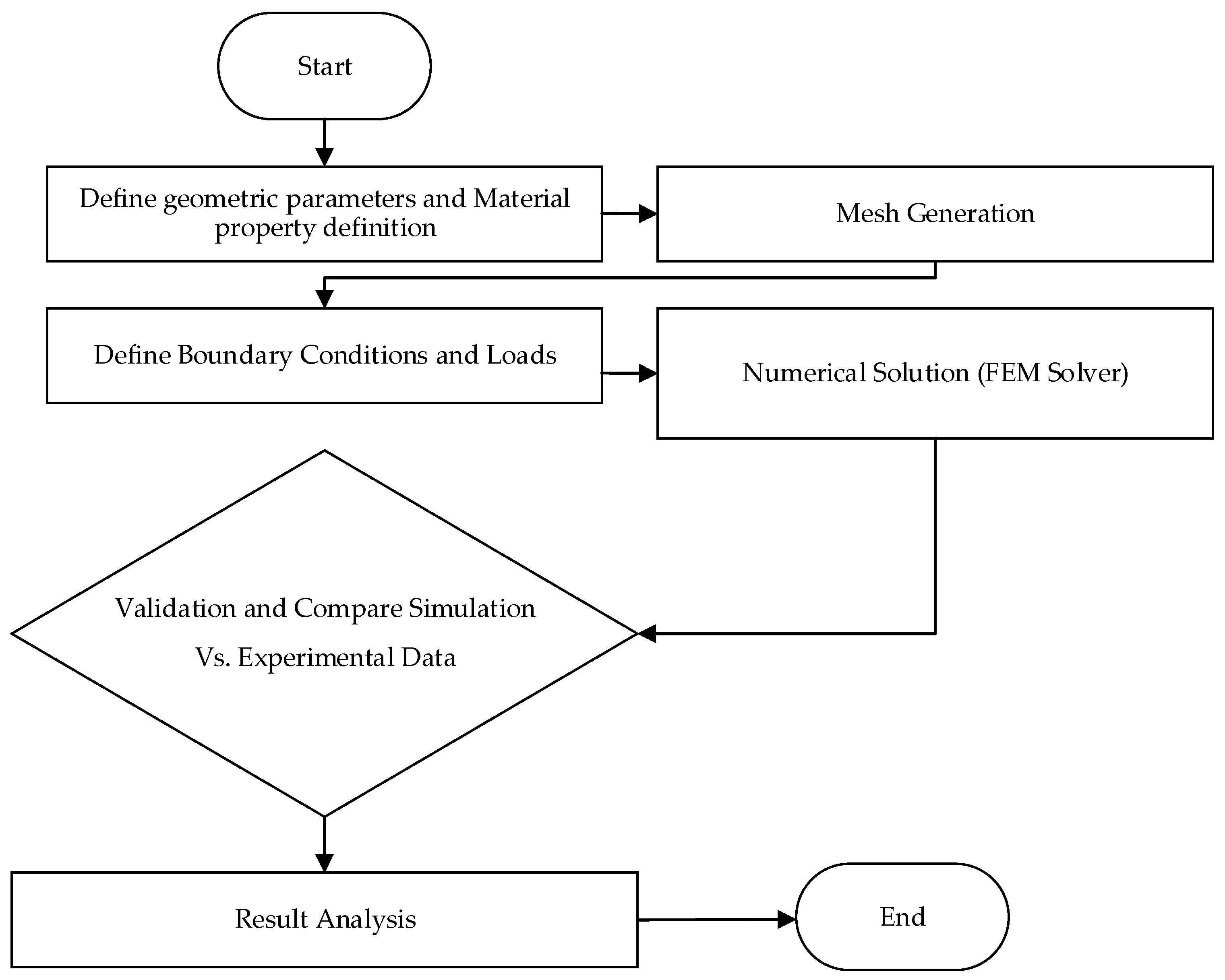
The computational framework employed in this study is illustrated in Figure 5. The procedure begins with the geometric modeling of the parabolic concentrator and receiver tube, followed by mesh generation. Material properties were defined with water density modeled as a temperature-dependent variable to capture thermal stratification effects.

Key boundary conditions were derived from field measurements: solar illuminance was converted into an equivalent volumetric heat generation rate to simulate the internal heat source. FEM solver then computed the steady-state solution for the convection-diffusion equation. Finally, the validity of the model was assessed by comparing the simulated maximum temperature and thermal gradients against the experimental prototype results.

3. Result of Solar Thermal

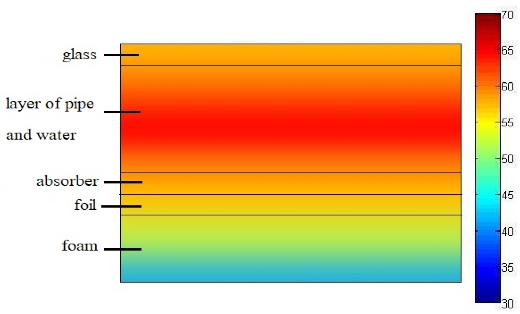
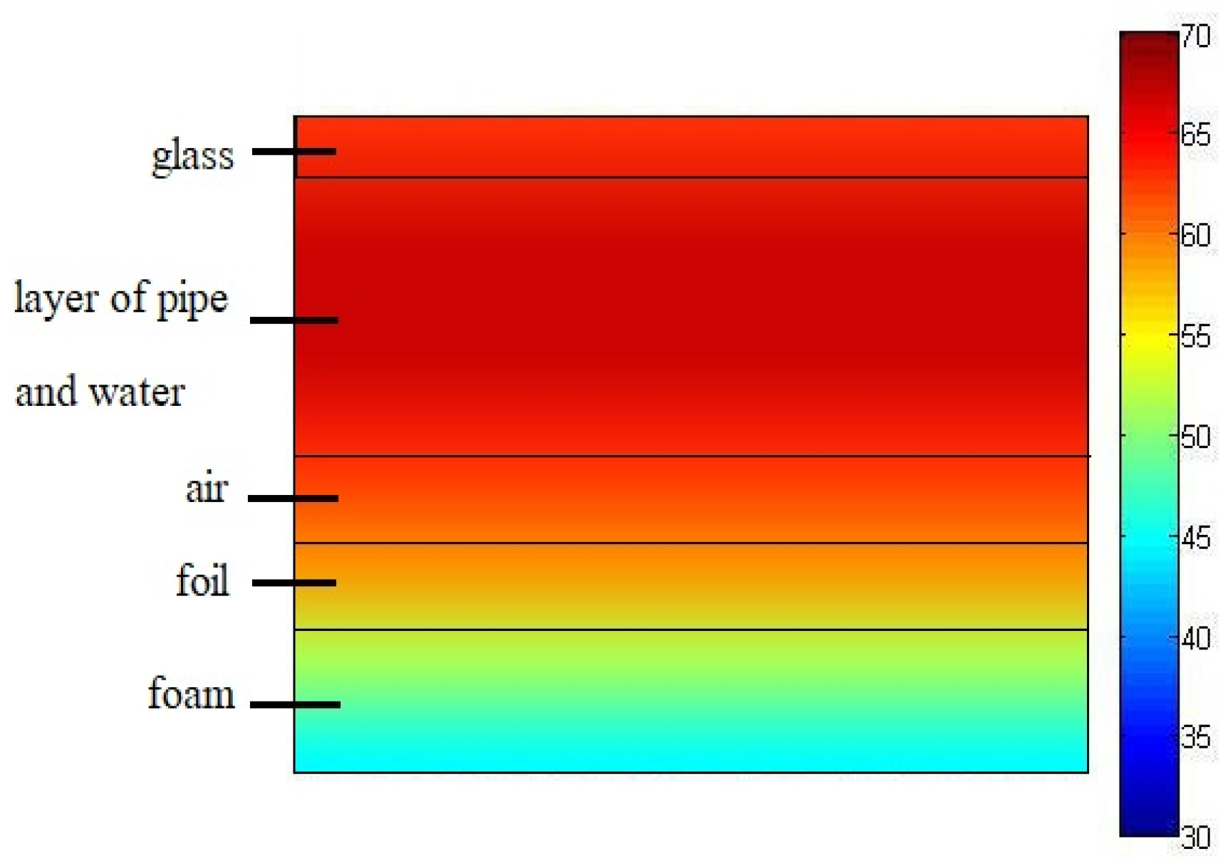
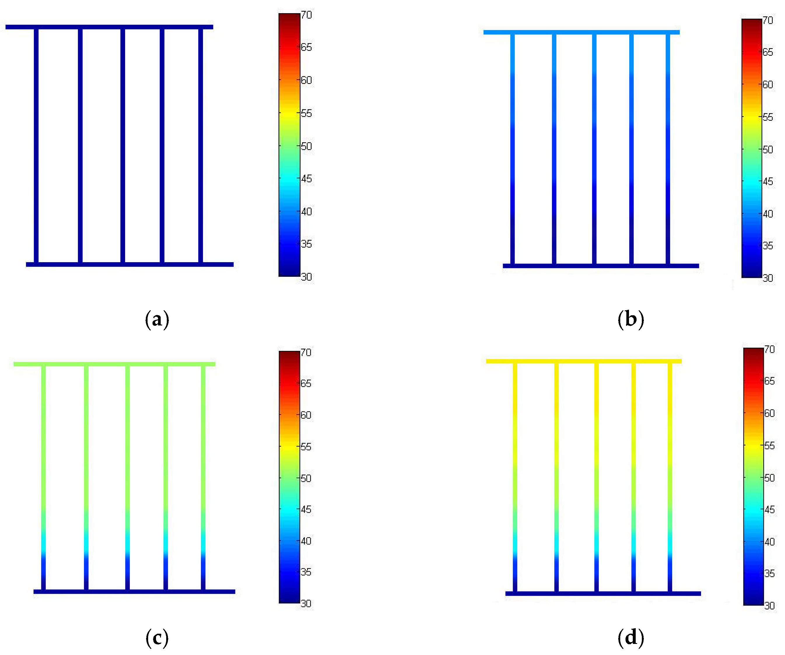
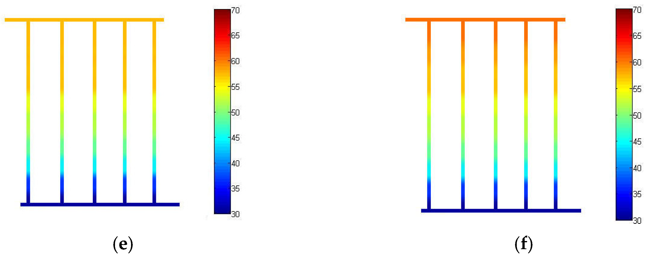
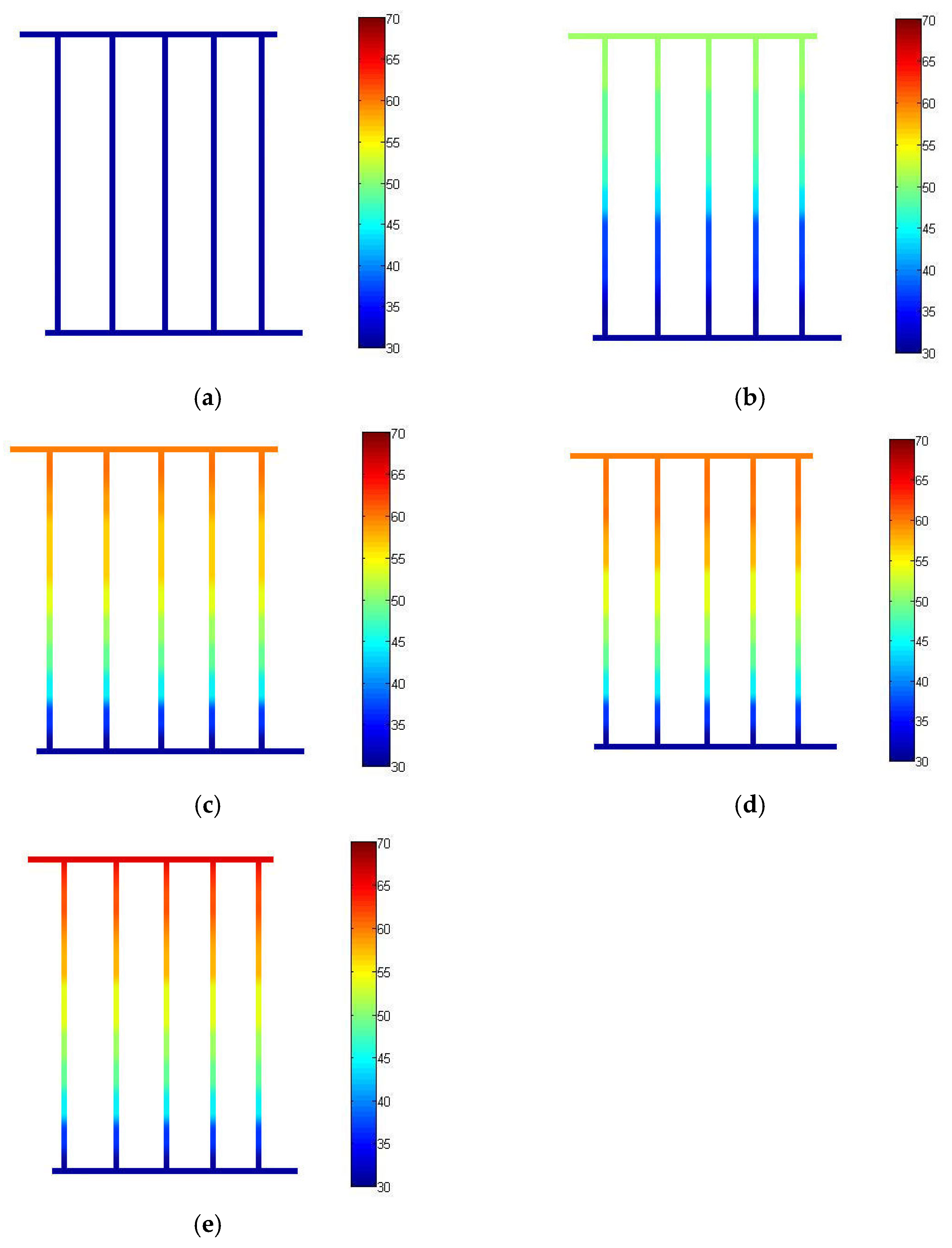
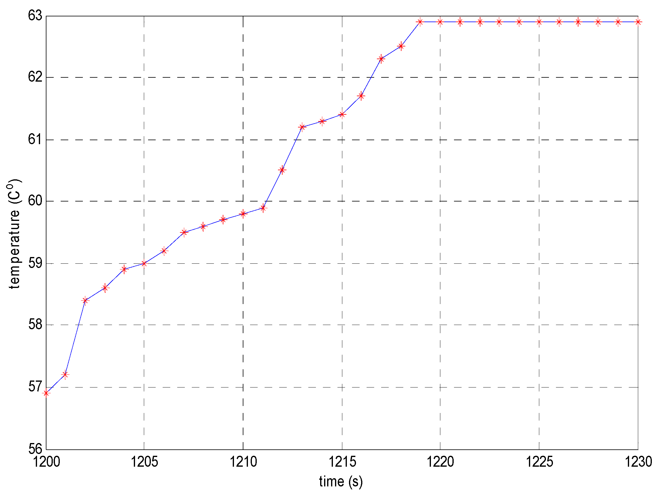
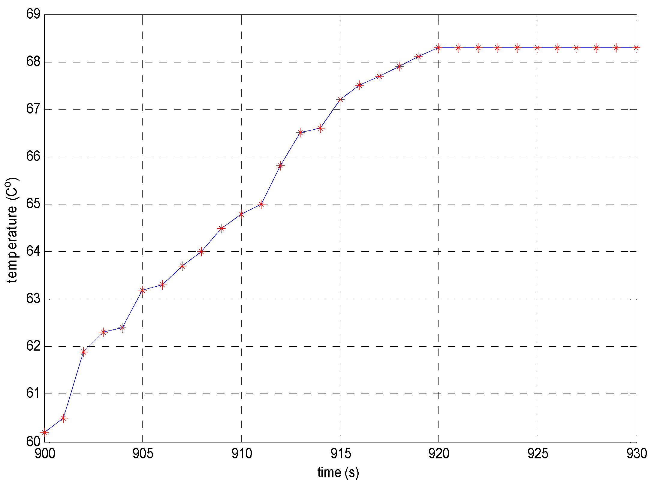
The paper’s FEM-based simulation is coded with MATLAB (Version R2024a) programming to calculate the temperature distribution in solar thermal systems. Figure 6 and Figure 7 illustrate the simulated temperature distributions for the conventional absorber and the proposed parabolic concentrator design, respectively. Figure 8 and Figure 9 depict the simulation result of temperature distribution in water when traditional solar thermal with absorber and novel solar thermal design with parabolic concentration are evaluated, respectively. Figure 10 and Figure 11 depict the simulation result of the maximum temperature distribution in water when traditional solar thermal with absorber is compared to the novel design of solar thermal with parabolic concentration. The simulation results of temperature comparison between conventional solar thermal with absorber and innovative solar thermal design with parabolic concentration are displayed in

Table 3. Comparison simulation result of temperature between traditional solar thermal with absorber and new design of solar thermal with parabolic concentration.

Material	Traditional Solar Thermal with Absorber		New Design of Solar Thermal with Parabolic Concentration
	Max Temperature (°C)	Min Temperature (°C)	Max Temperature (°C)	Min Temperature (°C)
Glass	58.1	56.3	63.1	63.4
Water	62.9	30	68.3	30
Absorber	61.4	57.7	-	-
Air	-	-	63.4	56.4
Foil	57.7	49.5	56.4	50.3
Foam	49.5	42.3	50.3	44.8

[20].

Figure 6 and Figure 7 compare the temperature distributions of the conventional and parabolic designs. In both configurations, temperatures rise from the glazing layer to the water core, where solar absorption leads to maximum fluid temperatures. The insulating layers (foil and foam) then induce a negative thermal gradient, reducing the temperature from the pipe wall down to the ambient condition (30 °C) at the system boundary.

Figure 8 and Figure 9 depict simulation results of temperature distribution in water when traditional solar thermal with absorber and new design of solar thermal with parabolic concentration are considered, indicating that when the water is released, the temperature does not change significantly because the heat accumulation is insufficient to transfer heat to the pipe. Yet, when heat accumulation is able to transfer heat to the pipe, the water will be replaced extremely rapidly. Water is in a stable state because it is constantly evaporating and being replaced by fresh water. The temperature will rise from the lower zone where water enters to the upper zone where it exits because heat is accumulated whenever water moves. Maximum water output temperature at steady state is 62.9 °C for classic solar thermal with absorber and 68.3 °C for the new solar thermal design with parabolic concentration.

Figure 10 and Figure 11 depict the simulation results of the maximum temperature distribution at the water outlet for the conventional solar thermal system with absorber and the new design of solar thermal with parabolic concentration, respectively, demonstrating that when heat is transferred to the pipe, the water will be rapidly changed. The water is then in a constant state since water continues to flow out, and new water will replace the old.

Table 3 compares the temperatures of conventional solar thermal absorbers and novel solar thermal concentration parabolic designs. The water temperature in the new solar thermal design with parabolic concentration is higher than in conventional solar thermal systems with absorber. Due to the rise in parabolic concentration rather than absorber, it concentrates internal heat production by accumulating heat at its focal point.

4. Designs of Solar Thermal Prototype for Experiment Result

4.1. Designs of Traditional Solar Thermal with Absorber

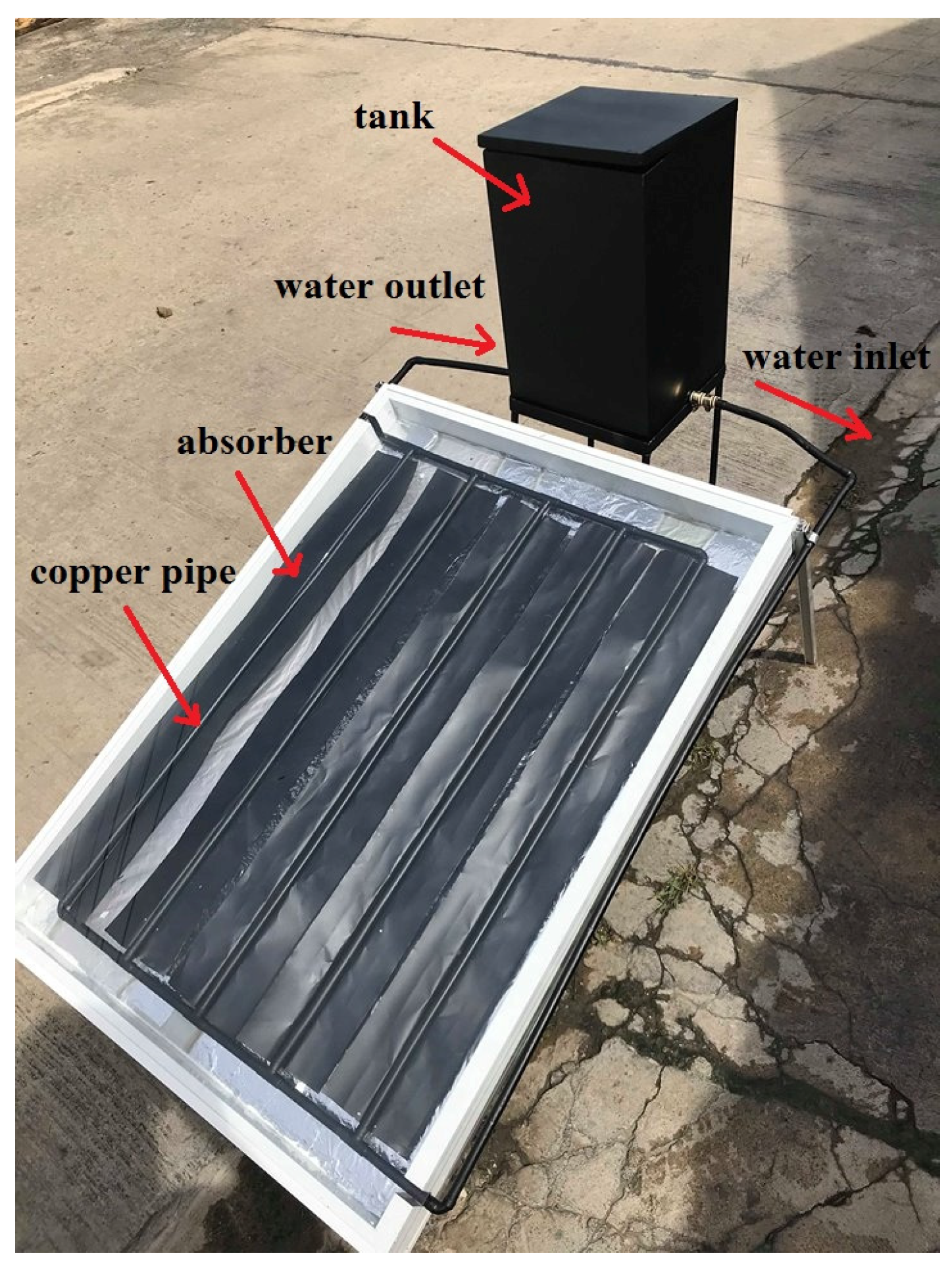
The diameter and length of a conventional solar thermal absorber are 700 mm and 1000 mm. The initial 3 mm-thick layer of glass prevents dust and heat loss. Pipe and water make up the second layer. The absorber sends heat to the pipe, which then transfers heat to the water. The pipe, which has a 16 mm diameter and a 2 mm wall thickness, transfers heat to the water. The third layer is an absorber that turns sunlight into fluid heat energy. Figure 12 demonstrates that the fourth layer is an insulated foil and the final layer is an insulating foam.

4.2. New Designs of Solar Thermal Prototype with Parabolic Concentration

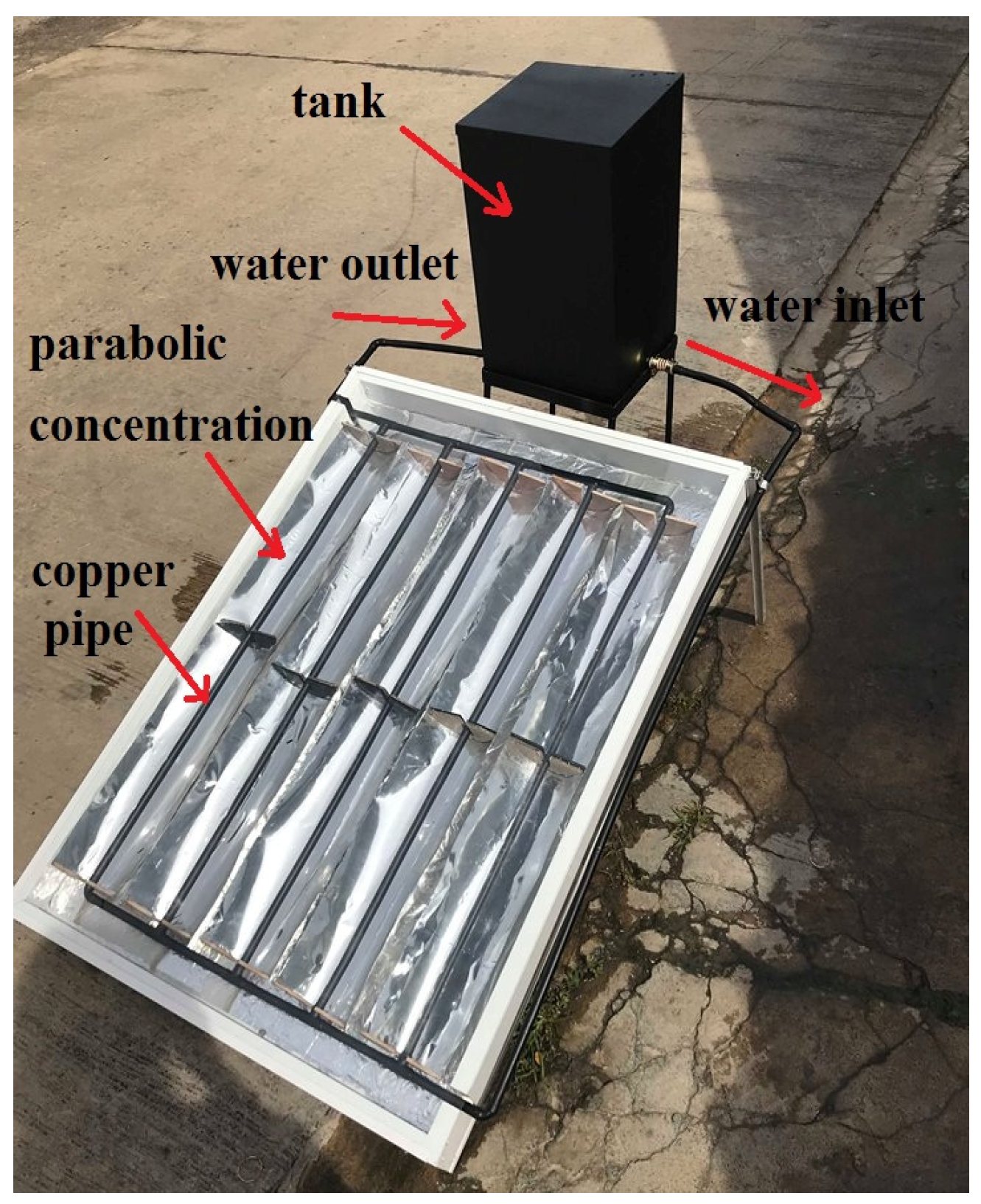
The new design of the solar thermal prototype with parabolic concentration has a width of 700 mm and a length of 1000 mm. The initial 3 mm-thick layer of glass prevents dust and heat loss. The second layer is a pipe and water with a 16 mm diameter and a 2 mm thickness. The design of the parabolic concentrator is based on the equation x² = 4cy, where c represents the focal length. The geometric parameters of the parabolic concentrator were determined using a constraint-based design approach rather than unconstrained optimization. The focal length (c = 2 cm) and aperture width were selected to satisfy two critical physical constraints: geometric fit: the concentrator array must fit within the fixed internal volume of the existing commercial water heater casing without overlapping edges; and manufacturability: the curvature must be feasible for manual fabrication using standard aluminum sheets (THAI WATSADU, Khon Kaen, Thailand). Therefore, the selected dimensions represent the most effective configuration achievable within the specific spatial limitations of the retrofit application. The third layer is a parabolic concentration that accumulates heat at the focal point to increase internal heat production. Figure 13 demonstrates that the fourth layer is an insulated foil and the final layer is an insulating foam.

4.3. Comparative Analysis with Recent Studies

When compared to the latest similar systems reported in referents, the proposed design offers distinct unique advantages. First, structural compactness: unlike the external, large-footprint collectors presented in [7], the proposed design integrates the parabolic concentrator internally within the water heater unit. This makes it suitable for residential retrofitting in limited spaces. Cost-effectiveness: while [6] utilized complex finned tubes which increase manufacturing costs, the proposed design employs a standard copper tube with a calculated optimal focal length. Simulation accuracy: by adapting the 3D FEM approach typically used in electromagnetics—a method distinct from the 1D/2D lumped parameter models often seen in the literature [1]—this study achieved a more precise prediction of the temperature gradient across the 3D geometry of the receiver.

5. Comparison of Simulation Results and Discussion

5.1. Comparative of Simulation Results

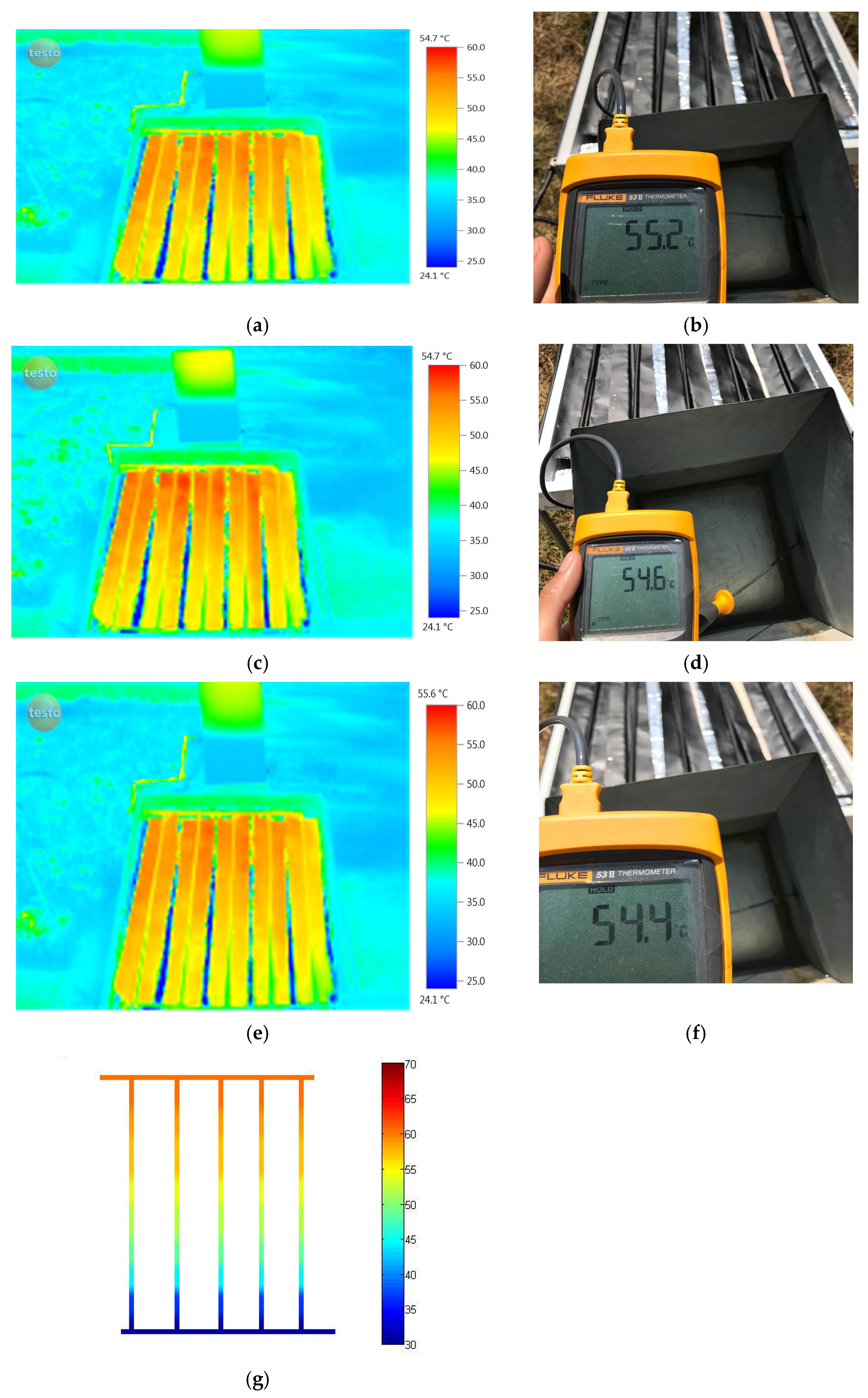
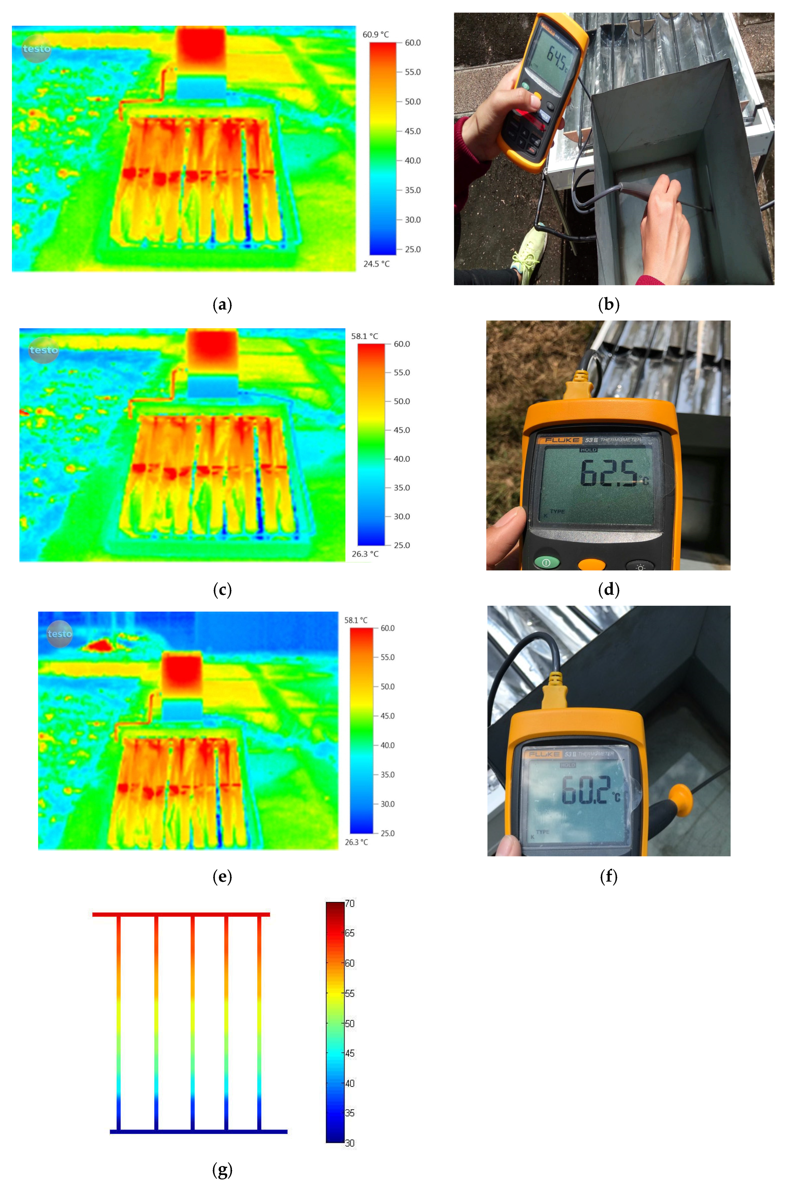
The results obtained from thermal imaging using a Testo 880 camera (Testo SE & Co. KGaA, Titisee-Neustadt, Germany) and thermocouples (Type K, Fluke 80PK-22 SureGrip™, Fluke Corporation, Everett, WA, USA) are compared with the simulation results. Figure 14 and Figure 15 show the simulation and experimental outcomes for the conventional solar thermal system with an absorber and the new solar thermal design with parabolic concentration, respectively. Additionally,

Table 4. Comparison of simulation results and experiment results when considered traditional solar thermal with absorber.

Condition	Simulation Result (°C)	Experiment Result (°C)
		Max Temperature from Thermal Image	Max Temperature from Thermocouple
First test	62.9	54.7	55.2
Second test	62.9	54.7	54.6
Third test	62.9	55.6	54.4
Average	62.9	55.0	54.7

and

Table 5. Comparison of simulation results and experiment results when considered new design of solar thermal with parabolic concentration.

Condition	Simulation Result (°C)	Experiment Result (°C)
		Max Temperature from Thermal Image	Max Temperature from Thermocouple
First test	68.3	60.9	64.5
Second test	68.3	58.1	62.5
Third test	68.3	58.1	60.2
Average	68.3	59.0	62.4

present a comparison between the simulated and experimental results for both the conventional solar thermal system with an absorber and the innovative parabolic concentration design, respectively. To ensure a fair comparison despite the lack of real-time solar irradiance control, both the conventional flat-plate absorber and the proposed parabolic concentrator were tested simultaneously under identical environmental conditions. This side-by-side arrangement minimizes the impact of fluctuating solar intensity and ambient variables on the comparative results.

5.2. Discussion

The comparative analysis (Figure 13 and Figure 14, Table 4 and Table 5) confirms the superior performance of the parabolic design over the conventional absorber. The concentrator intensifies heat generation at the focal point, driving thermal stratification where lower-density hot water naturally accumulates at the upper sections. A maximum discrepancy of approximately 8 °C (26% thermal gradient deviation) was observed, primarily attributed to the exclusion of radiative heat losses in the simplified FEM model. Unlike high-fidelity multiphysics models [21] that achieve <0.1% error using complex electromagnetic-thermal coupling, this study employs a simplified approach specifically strictly for preliminary prototyping of low-cost retrofits. Although absolute temperatures are overestimated, the model successfully captures the relative thermal enhancement trends, validating the feasibility of the parabolic design.

Statistical Error Analysis. To quantitatively evaluate the accuracy of the FEM simulation against the experimental data, statistical metrics including the Root Mean Square Error (RMSE) and the coefficient of determination (R²). The calculated RMSE was 6.8 °C, representing the average magnitude of the prediction error. Despite the absolute discrepancy caused by neglecting radiative losses, the coefficient of determination R² was found to be 0.95, indicating a very strong correlation between the simulated trends and the experimental measurements. These statistical values indicate that the simplified model is adequate for predicting the relative thermal performance of the parabolic design.

To verify whether the neglected radiative heat loss is physically consistent with the observed ~8 °C deviation between the simulation and experimental results, a simplified analytical estimation was performed using the Stefan–Boltzmann law. The radiative heat transfer rate (Q_rad) from the receiver tube to the ambient environment can be approximated as

$$Q_{rad}=\epsilon \sigma A\left(T_s^4-T_{amb}^4\right).$$

(15)

Using the operational parameters (e.g., T_S ≈ 338 K or 65 °C and T_amb ≈ 303 K or 30 °C), the estimated radiative heat loss over the experimental duration corresponds to a specific amount of unreleased thermal energy. When this unaccounted energy is applied to the sensible heat equation (Q = mC_p∆T) for the specific mass of water in the system, it yields a theoretical temperature difference (∆T) of approximately 7 to 9 °C. This order-of-magnitude validation quantitatively confirms that the ~8 °C overestimation in the FEM model is directly and physically attributable to the exclusion of the thermal radiation term.

A qualitative sensitivity analysis was considered to evaluate the model’s robustness against variations in key parameters, namely solar input, convective coefficient, and surface emissivity. Analytically, fluctuations in solar irradiance directly shift the maximum heat generation, while variations in the convective and radiative boundaries (emissivity) alter the heat dissipation rates. These boundary effects account for the ~8 °C absolute temperature overestimation observed in the simulation. However, while such parameter variations affect the absolute peak temperatures, the relative thermal gradients across the collector layers and the comparative enhancement of the parabolic design remain highly consistent. Consequently, despite the modeling simplifications, the overall thermal behavior and the primary conclusions of this study are fundamentally robust.

The current model relies on the following simplifying assumptions:

• Radiative Heat Loss: The exclusion of surface-to-ambient radiation in the FEM model resulted in a slight overprediction of temperatures (~ 8 °C deviation).
• Solar Input Approximation: The heat generation rate was derived from illuminance data rather than direct pyranometer readings, serving as an approximation of solar irradiance.
• Environmental Stability: Dynamic outdoor conditions (e.g., variable wind speed) were modeled as constant parameters.

6. Conclusions

This study successfully conducted a preliminary engineering validation of a redesigned solar water heater integrating an internal stationary parabolic concentrator. Operating under a constrained-design framework, the application of the simplified 3D-FEM allowed for the practical prediction of thermal distribution trends, which were subsequently compared against experimental prototype data.

Key findings from the study are as follows:

• The simulation model predicted a maximum water temperature of 62.9 °C at the focal zone.
• The experimental prototype, tested under corresponding field conditions, achieved a maximum water temperature of 55.0 °C.
• The comparative analysis reveals an absolute temperature error of 7.9 °C (a relative error of approximately 12.5%). The physical implication of this overestimation is primarily attributed to external boundary simplifications in the numerical model, specifically the neglect of surface-to-ambient radiative heat losses.
• Furthermore, a thermal gradient deviation of approximately 26% was observed when comparing the temperature drop across the collector layers. Physically, this discrepancy implies variations in internal thermal transport, likely due to unmodeled contact resistances between the physical components (e.g., pipe and absorber) and the simplified natural convection dynamics within the fluid.

Despite these specific deviations, the thermal behavior trends between simulation and experiment remain consistent. The results confirm that the proposed parabolic design significantly increases the heat generation rate compared to the conventional flat-plate baseline. Future work will focus on incorporating surface-to-surface radiation into the FEM model to reduce the prediction error and conducting a long-term economic feasibility analysis.

References

1. Grena, R.; Lanchi, M.; Frangella, M.; Ferraro, V.; Marinelli, V.; D’Auria, M. Thermal Analysis of Parabolic and Fresnel Linear Solar Collectors Using Compressed Gases as Heat Transfer Fluid in CSP Plants. Energies 2024, 17, 3880. [Google Scholar] [CrossRef] [Scilit]
2. Kong, L.; Niu, Y.; Fan, D.; Shi, M.; Zheng, Z. Numerical Simulation Analysis of the Temperature Field of Molten Salt Linear Fresnel Collector. Energies 2025, 18, 5815. [Google Scholar] [CrossRef] [Scilit]
3. Maatallah, T.; Houcine, A.; Saeed, F.; Khan, S.; Ali, S. Simulated Performance Analysis of a Hybrid Water-Cooled Photovoltaic/Parabolic Dish Concentrator Coupled with Conical Cavity Receiver. Sustainability 2024, 16, 544. [Google Scholar] [CrossRef] [Scilit]
4. Can, O.F.; Celik, N.; Ozgen, F.; Kistak, C.; Taskiran, A. Experimental and Numerical Analysis of the Solar Collector with Stainless Steel Scourers Added to the Absorber Surface. Appl. Sci. 2024, 14, 2629. [Google Scholar] [CrossRef] [Scilit]
5. Bunmat, A.; Saikham, P.; Siripat, T.; Thuaythungsa, A.; Pao-la-or, P. Simulation of Electromagnetic Field of Electrical Conductor Materials in Wireless Charging Device Using 3D Finite Element Method. Int. Rev. Model. Simul. 2025, 18, 1–8. [Google Scholar] [CrossRef] [Scilit]
6. Limboonruang, T.; Oyinlola, M.; Harmanto, D.; Bunyawanichakul, P.; Phunapai, N. Optimizing Solar Parabolic Trough Receivers with External Fins: An Experimental Study on Enhancing Heat Transfer and Thermal Efficiency. Energies 2023, 16, 6520. [Google Scholar] [CrossRef] [Scilit]
7. Mahdhi, J.; Hamdi, F.; Ebadi, H.; Bouabidi, A.; Ennetta, R.; Savoldi, L. Experimental Study of a Stationary Parabolic Trough Collector with Modified Absorbers for Domestic Water Heating. Energies 2025, 18, 3261. [Google Scholar] [CrossRef] [Scilit]
8. Arun, M.; Barik, D.; Ahmad, H.; Alraddadi, I.; Shenashen, M.A.; Khan, Z.A. Parabolic trough solar collector technology using TiO2 nanofluids with dimpled tubes. Case Stud. Therm. Eng. 2024, 61, 104840. [Google Scholar] [CrossRef] [Scilit]
9. Arif, M.N.; Waqas, A.; Butt, F.A.; Mahmood, M.; Khoja, A.H.; Ali, M.; Ullah, K.; Mujtaba, M.A.; Kalam, M.A. Techno-economic assessment of solar water heating systems for sustainable tourism in northern Pakistan. Alex. Eng. J. 2022, 61, 5485. [Google Scholar] [CrossRef] [Scilit]
10. Barrón-Díaz, J.E.; Flores-Johnson, E.A.; Chan-Colli, D.G.; Koh-Dzul, J.F.; Bassam, A.; Patiño-Lopez, L.D.; Carrillo, J.G. FEM-CFD Simulation and Experimental Study of Compound Parabolic Concentrator (CPC) Solar Collectors with and without Fins for Residential Applications. Appl. Sci. 2021, 11, 3704. [Google Scholar] [CrossRef] [Scilit]
11. Lewis, R.W.; Nithiarasu, P.; Seetharamu, K.N. Fundamentals of the Finite Element Method for Heat and Fluid Flow; John Wiley & Sons: Hoboken, NJ, USA, 2004. [Google Scholar]
12. Bhatti, M.A. Advanced Topics in Finite Element Analysis of Structures; John Wiley & Sons: Hoboken, NJ, USA, 2006. [Google Scholar]
13. Kattan, P.I. MATLAB Guide to Finite Elements, 2nd ed.; Springer: Berlin/Heidelberg, Germany, 2007. [Google Scholar]
14. Jabbar, M.A.; Phyu, H.N.; Liu, Z.J.; Bi, C. Modeling and numerical simulation of a brushless permanent-magnet dc motor in dynamic conditions by time-stepping technique. IEEE Trans. Ind. Appl. 2004, 40, 763–769. [Google Scholar] [CrossRef]
15. Kaloudis, E.; Grigoriadis, D.G.E.; Papanicolaou, E.; Panidis, T. Large eddy simulations of turbulent mixed convection in the charging of a rectangular thermal storage tank. Int. J. Heat Fluid Flow 2013, 44, 776–791. [Google Scholar] [CrossRef] [Scilit]
16. Sheeba, J.B.; Rohini, A.K. Structural and thermal analysis of asphalt solar collector using finite element method. J. Energy 2014, 2014, 602087. [Google Scholar] [CrossRef] [Scilit]
17. Russel, Y. The effect of natural convection on viscous-flow heat transfer in horizontal tubes. Chem. Eng. Sci. 2013, 17, 335–350. [Google Scholar]
18. Yu, Y.J.; Masahiro, S.; Masashi, N. Boundary condition effects on the flow stability in toroidal thermosyphon. Int. J. Heat Fluid Flow 2002, 23, 81–91. [Google Scholar] [CrossRef] [Scilit]
19. Sparrow, E.M.; Gregg, J.L. Laminar free convection from a vertical plate with uniform heat flux. ASME J. Heat Transf. 1956, 75, 435–440. [Google Scholar] [CrossRef] [Scilit]
20. Dinsenmeyer, R.; Fourmigué, J.F.; Caney, N.; Marty, P. Volume of fluid approach of boiling flows in concentrated solar plants. Int. J. Heat Fluid Flow 2017, 65, 177–191. [Google Scholar] [CrossRef] [Scilit]
21. Stebel, M.; Kubiczek, K.; Rodriguez, G.R.; Palacz, M.; Garelli, L.; Melka, B.; Haida, M.; Bodys, J.; Nowak, A.J.; Lasek, P.; et al. Thermal analysis of 8.5 MVA disk-type power transformer cooled by biodegradable ester oil working in ONAN mode by using advanced EMAG–CFD–CFD coupling. Int. J. Electr. Power Energy Syst. 2022, 136, 107737. [Google Scholar] [CrossRef] [Scilit]
Figure 1. Detail of traditional solar thermal with absorber: (a) traditional solar thermal with absorber; (b) each layer; (c) pipe and water.
Energies 19 01182 g001
Figure 2. Mesh of traditional solar thermal with absorber: (a) traditional solar thermal with absorber; (b) pipe and water.
Energies 19 01182 g002
Figure 3. Detail of the new design of solar thermal with parabolic concentration: (a) the new design of solar thermal with parabolic concentration; (b) each layer; (c) pipe and water.
Energies 19 01182 g003
Figure 4. Mesh of the new design of solar thermal with parabolic concentration: (a) the new design of solar thermal with parabolic concentration; (b) pipe and water.
Energies 19 01182 g004
Figure 5. Simulation flowchart.
Energies 19 01182 g005
Figure 6. Simulation result of temperature distribution in solar thermal when considered traditional solar thermal with absorber (°C).
Energies 19 01182 g006
Figure 7. Simulation result of temperature distribution in solar thermal when considered new design of solar thermal with parabolic concentration (°C).
Energies 19 01182 g007
Figure 8. Simulation result of temperature distribution in water when considered traditional solar thermal with absorber (°C): (a) 0 s; (b) 300 s; (c) 600 s; (d) 900 s; (e) 1200 s; (f) 1220 s.
Energies 19 01182 g008aEnergies 19 01182 g008b
Figure 9. Simulation result of temperature distribution in water when considered new design of solar thermal with parabolic concentration (°C): (a) 0 s; (b) 300 s; (c) 600 s; (d) 900 s; (e) 1200 s.
Energies 19 01182 g009
Figure 10. Simulation result of maximum temperature distribution which is the water outlet when considered traditional solar thermal with absorber (°C).
Energies 19 01182 g010
Figure 11. Simulation result of maximum temperature distribution which is the water outlet when considered new design of solar thermal with parabolic concentration (°C).
Energies 19 01182 g011
Figure 12. Traditional solar thermal with absorber.
Energies 19 01182 g012
Figure 13. New designs of solar thermal prototype with parabolic concentration.
Energies 19 01182 g013
Figure 14. Simulation result and experimental result when considered traditional solar thermal with absorber: (a) first experiment result from thermal image; (b) first experiment result from thermocouple; (c) second experiment result from thermal image; (d) second experiment result from thermocouple; (e) third experiment result from thermal image; (f) third experiment result from thermocouple; (g) simulation result.
Energies 19 01182 g014
Figure 15. Simulation result and experimental result when considered new design of solar thermal with parabolic concentration: (a) first experiment result from thermal image; (b) first experiment result from thermocouple; (c) second experiment result from thermal image; (d) second experiment result from thermocouple; (e) third experiment result from thermal image; (f) third experiment result from thermocouple; (g) simulation result.
Energies 19 01182 g015