Optimal Linear Feedback Control—OLFC Applied to a Small Turbine Operating in Region II

Abstract

Wind energy production is growing year after year, increasing the share of wind energy in global energy sources. The amount of energy obtained depends on the wind speed. When wind speeds are below the nominal value, the goal is to maximize energy production. To optimize energy extraction under these conditions, the study employs the optimal torque (OT) control method in combination with the Optimal Linear Feedback Control (OLFC) technique. Although the OLFC method was developed some time ago, the literature has not yet thoroughly explored its application to wind turbines. This work aims to evaluate the dynamic response and energy output of a small-scale wind turbine equipped with an OLFC. Performance is evaluated relative to the uncontrolled system. The results demonstrate that the turbine controlled by the OLFC strategy maintained optimal operating conditions throughout the evaluation period under all wind scenarios. In contrast, the uncontrolled turbine exhibited inferior performance and failed to achieve the desired optimal parameters. The controlled turbine also shows a higher generated power than the uncontrolled turbine across all evaluated wind conditions. The OLFC technique demonstrated satisfactory performance, was simple to implement, and did not require system linearization.

1. Introduction

In 2020, the total installed electricity generation capacity from renewable energy sources was 111% higher than in 2010 [1]. In 2024, 90% of all expansion in the electricity sector was in renewable energy, with 20% of this growth driven by wind energy [2]. Projections indicate that total installed capacity will reach 18,000 GW by 2050, with solar and wind energy sources accounting for 77.78% of this capacity [2]. Wind energy plays a prominent role due to availability and potential for deployment across many regions of the world [3]. In addition, wind energy is versatile and modular. The installation of large-scale wind turbines, with power ratings above 1 MW, can significantly affect the surrounding environment [4]. The use of small-scale wind turbines, capable of generating up to 10 kW, represents a less environmentally intrusive alternative [4].

Wind turbines are rotating machines that capture a portion of the wind’s kinetic energy and convert it into electrical energy. As the wind flows over the turbine blades, it exerts aerodynamic forces that produce rotational kinetic energy in the rotor shaft. A gearbox typically connects to the rotor shaft. It increases its rotational speed and transmits to the generator shaft at the appropriate operating speed. The generator then converts the available rotational kinetic energy into electrical energy using magnetic fields and delivers it to the electrical grid.

Horizontal-axis wind turbines (HAWTs) are the dominant configuration [5]. They offer considerable advantages, such as improved aerodynamic performance, balanced transmission loads, and lower cost. The HAWT with a three-bladed rotor has become the current industry standard [6].

In the past, wind turbines were operated at a fixed speed. Technological advancements over the past few decades have enabled variable-speed operation. It is possible to adjust the rotor’s rotation speed to match variations in wind speed [6]. This type of operation is advantageous because it allows for maximizing energy production and reducing mechanical stress and power fluctuations [6,7,8].

Small-scale wind turbines typically use a horizontal-axis, three-bladed rotor configuration. Depending on the generator type, they may operate with or without a gearbox. Permanent magnet synchronous generators (PMSGs) and induction generators (IGs) are the most commonly used [6]. PMSGs are used for their greater efficiency, better performance, and greater ability to remain operational during fault passages [6]. Variable-speed turbines commonly use induction generators (IGs) with power electronic converters. Their lower cost primarily justifies their adoption compared with alternative generator technologies. However, the use of an IG requires a gearbox and external excitation supply [6]. The IGs allow the turbine rotor speed to vary by approximately ±30% around the generator synchronous speed [9,10].

Variable-speed wind turbines operate in four distinct regions [4,7,8,11,12,13,14]. Region I occurs when the wind speed is less than or equal to the cut-in speed ($V_{cut\text{-}in}$) required for starting. Under these conditions, the torque developed in the rotor is less than the torque required to start the turbine and produce energy. Therefore, the turbine remains stationary. For this reason, the turbines remain off. The equipment begins operating at wind speeds greater than $V_{cut\text{-}in}$. This is the beginning of Region II, which extends to the rated wind speed ($V_{rated}$). The objective is to achieve the condition that maximizes wind energy conversion. This is generally done using maximum power point tracking (MPPT). The next operating region is Region III. It starts at wind speeds greater than $V_{rated}$ and extends to the cut-off speed ($V_{cut\text{-}off}$). The objective is to regulate power output to prevent exceeding the system’s operational limits. The control action used in this region is generally the adjustment of the blade pitch angle ($\beta$). The controller defines the angle according to the wind speed. The last operational region is Region IV. It starts the instant the wind speed exceeds $V_{cut\text{-}off}$. The equipment is then shut down to prevent damage.

It is needed to improve energy capture efficiency to make wind power generation more competitive. Wind power extraction depends on the power coefficient ($C_P$), which is influenced by the tip-speed ratio ($\lambda$) and the blade pitch angle ($\beta$). In Region II, the objective is to maximize wind energy extraction. The optimal tip-speed ratio (${\lambda }_{opt}$) and the optimal blade pitch angle (${\beta }_{opt}$) define the optimal operating conditions. The control system maintains the rotor blades at ${\beta }_{opt}$ while varying the rotor speed according to the MPPT procedure. It ensures that the rotor attains ${\lambda }_{opt}$ at any wind speed. The MPPT procedure can be used in any wind turbine [13]. Turbine performance is influenced by the control system used in the MPPT strategy [6]. The MPPT procedure identifies the optimal operating point using measured parameters, such as wind speed, generator shaft speed, or generated power [9]. The system compares the measured values with their optimal references and sends a control signal to the controller, which adjusts generator operation [15].

A wide variety of MPPT control methods are available in the literature. The most well-known MPPT methods are tip speed ratio (TSR), perturb-and-observe (P&O), and optimal torque (OT) [6,16].

The TSR method determines the rotor rotational speed required to maintain ${\lambda }_{opt}$ for the current wind speed [16]. The control system obtains the signal from the difference between the measured rotor shaft speed and the reference defined by the TSR procedure. The controller adjusts the generator torque, thereby modifying the generator rotational speed and, consequently, the rotor speed. The application of the TSR method is limited by its higher cost and by the requirement for accurate wind speed measurements [16].

The P&O method uses measured variations in generated power relative to the known turbine power curve to adjust rotor speed [16]. The method responds rapidly to instantaneous wind variations, which may cause unnecessary changes in rotor speed and oscillations in the MPPT process [16].

The OT adjusts the generator torque to achieve the reference value, based on the generator shaft rotational speed. A quadratic law of the generator speed determines the reference generator torque. It is necessary to know the rotor’s aerodynamic parameters. One limitation of the OT method is its inability to adjust rotor speed rapidly in response to wind speed variations, which negatively affects MPPT performance [17]. Researchers proposed several improvements to accelerate the MPPT process, developing methods that improved optimal torque, decreased torque gain, and adaptive torque gain [16]. Although these approaches improve MPPT performance, engineers face difficulties in tuning their parameters. In addition, it can enhance OT performance by combining it with neural networks and fuzzy logic controllers [6].

In addition to the MPPT methods already presented, other methods have been developed, including sliding mode control, linear-quadratic-Gaussian control, and nonlinear control, $H_{\infty }$ control, model predictive control [9]. Recently, reinforcement learning techniques have also improved MPPT control methods by adapting to system changes and effectively handling uncertainties and disturbances [18]. A review of control method strategies for region II and the MPPT strategy was conducted by [6,12,19,20]. Sophisticated MPPT methods provide better performance but require high-processing-capability hardware [16]. When used without such resources, it causes convergence and performance problems [16].

The OT is the primary approach employed in wind turbines due to its ease of implementation [16,21]. When applied to small wind turbines, it delivers satisfactory performance. In this work, we adopt OT control with an MPPT strategy for wind turbine operation in Region II.

Many researchers have successfully applied optimal control strategies to wind turbines. The linear quadratic regulator (LQR) with optimal gain scheduling demonstrates greater stability, faster response, and higher accuracy than conventional controllers [22]. The combined back-stepping and LQR control demonstrates improved robustness and performance, as well as enhanced power quality and stability [23]. In [24], an improved LQR is presented for controlling the two-mass model of a wind turbine. The proposed controller achieved better performance and reduced fluctuations in generated power when compared with conventional controllers.

The OLFC is an extension of the LQR for problems involving nonlinear systems [25,26]. Some researchers have successfully employed the OLFC controller. It was applied to a microelectromechanical system, achieving robust trajectory tracking without requiring linearization or elimination of the system nonlinearities [27,28]. In [29], researchers used OLFC to stabilize an atomic force microscopy mechanism along a predefined orbit, achieving good tracking performance and robustness under parametric error analysis. In [30], OLFC stabilized chaotic motion on a predefined periodic orbit to synchronize a Lorenz system, achieving high accuracy with minimal trajectory errors and low computational cost. Additionally, in [31], researchers applied OLFC to drive an energy production system along the desired trajectory, obtaining low tracking error relative to the reference trajectory.

This work aims to evaluate the performance of the OLFC technique combined with OT for a small wind turbine operating in region II. We assess the OLFCler’s ability to achieve MPPT. We analyze the state error behavior throughout the entire simulation time. We use four different wind conditions in our analyses: stepwise increase in wind speed, linear ramp in wind speed, rapid gusts, and turbulent wind. We also verify the optimal operating condition of the OLFC controller in each wind condition. The energy produced during the simulation for each wind condition was determined. This value allows the extrapolation of annual energy production in each situation. The annual energy production gains using OLFC control were determined. Finally, we discuss the limitations of this work and suggest opportunities for further development.

We have structured this work into five sections. Section 2 discusses the aerodynamic and mechanical model of the wind turbine in detail. Section 3 discusses the OLFC technique and develops the controller design in detail. Section 4 presents the simulation definitions and parameters of the small wind turbine and the four wind profiles used. Section 5 presents and analyzes the results obtained. Also, we discuss the limitations of this study. Finally, this work presents conclusions and suggestions for future work.

2. Mathematical Modeling of a Small Wind Turbine

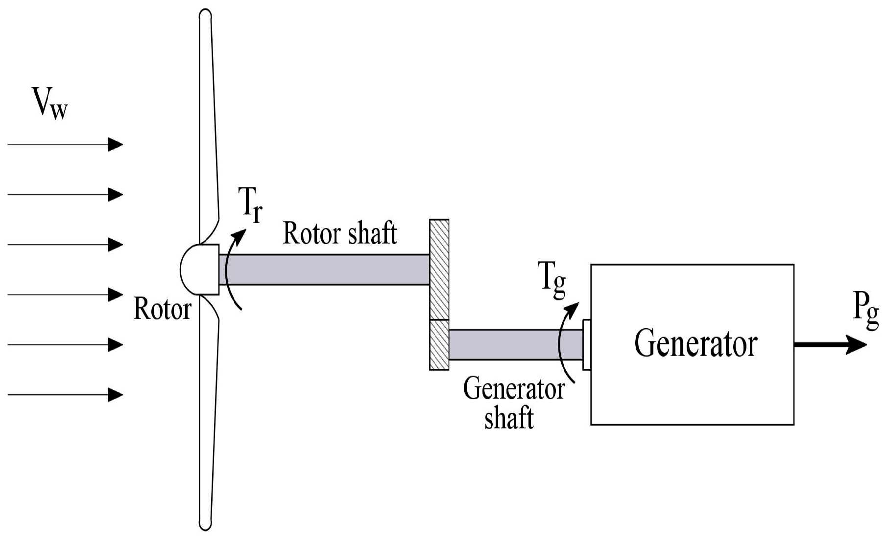
The modern wind turbines consist of three subsystems: aerodynamic, mechanical, and electrical [32,33,34,35,36]. The aerodynamic subsystem is the rotor, which converts wind energy into rotor torque ($T_r$). The mechanical subsystem consists of a shaft that connects the rotor to the gears, which increase the rotation speed for the shaft connected to the generator, delivering generator torque ($T_g$). The final subsystem is the generator’s electrical system, which converts the mechanical energy of the shaft rotation into electrical power. Figure 1 shows a schematic representation of a typical wind turbine.

2.1. Aerodynamic of Wind Turbine

Aerodynamics is an important point in the construction of a mathematical model of a wind turbine. Large wind turbines have long, flexible blades that interact significantly with the wind [37,38]. In recent years, CFD (Computational Fluid Dynamics) and aeroelastic models have been employed in large turbines [17,36,39,40,41,42,43,44].

However, it requires more computational resources. Small turbines have blades that are smaller than those of large turbines and therefore less flexible. A simplified aerodynamic model has been widely used in some projects [4,11,12,33,45,46,47,48]. The simplified model assumes a rigid rotor. The model disregards aerodynamic instability and aeroelastic interactions.

The simplified aerodynamic model uses non-linear expressions for power. The accuracy is directly related to the uncertainties involved in the $C_P$ expressions [4,11,12,33,45,46,47,48]. The focus of this work is on the application of the OLFC controller and its performance in small-scale wind turbine systems. This work employs the simplified aerodynamic model. The simplified model is presented below.

According to [11,33,36,45,46,49,50], the rotor converts wind power into mechanical power ($P_r$) by:

$$P_r={\displaystyle \frac{1}{2}}{\rho }_{air} \pi R^2 C_P\left(\lambda ,\beta \right) V_w^3,$$

(1)

${\rho }_{air}=1.225 {\displaystyle \raisebox{1ex}{$\mathrm{k}\mathrm{g}$}\!\left/ \!\raisebox{-1ex}{${\mathrm{m}}^3$}\right.}$, $R$ is the radius of the rotor and $V_w$ is the wind speed at the height of the rotor. The $C_P\left(\lambda ,\beta \right)$ is influenced by $\beta$ and $\lambda$, the latter defined by

$$\lambda ={\displaystyle \frac{R {\omega }_r}{V_w}},$$

(2)

${\omega }_r$ is the rotor speed shaft. The relationship between the rotor shaft’s rotational mechanical power and the torque developed by the rotor as

$$T_r={\displaystyle \frac{P_r}{{\omega }_r}}={\displaystyle \frac{1}{2}}{\rho }_{air} \pi R^3{ C}_P\left(\lambda ,\beta \right){ V}_w^2,$$

(3)

the $C_P\left(\lambda ,\beta \right)$ indicates the capacity to convert wind energy into mechanical energy. Theoretical considerations limit it to the Betz limit [10,51]. The $C_P\left(\lambda ,\beta \right)$ reaches its maximum value $C_{P,max}$ at a specific operating point defined by ${\lambda }_{opt}$ and ${\beta }_{opt}$. The rotor blade geometry determines the optimal values of these parameters. At the maximum operating point, the rotor develops its maximum torque $\left(T_{r,max}\right)$, given by

$$T_{r,max}={\displaystyle \frac{1}{2}}{\rho }_{air} \pi R^5{\displaystyle \frac{C_{P,max}}{{\lambda }_{opt}^3}} {\omega }_r^2,$$

(4)

2.2. Simplified Mechanical Model

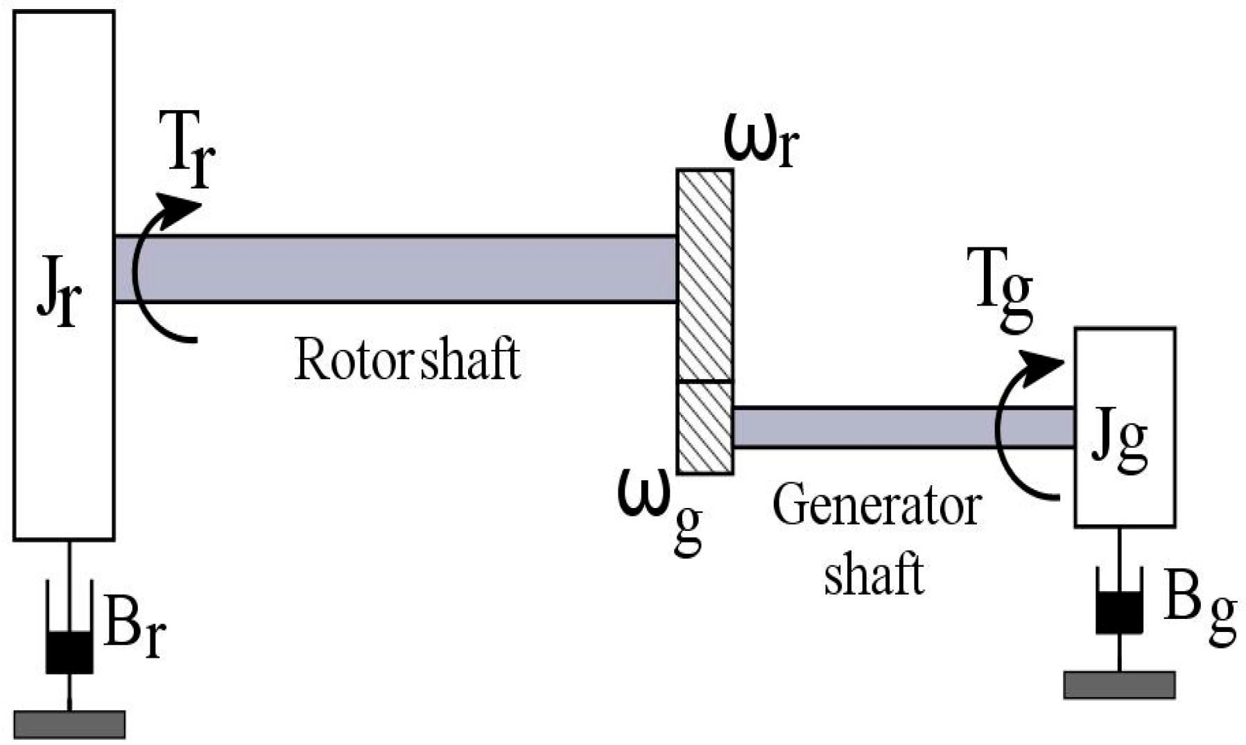
Figure 2 shows a simplified dynamic model of a wind turbine. This model including rotor’s shaft, gears, and generator [7,10,32,33,41,47,48,52,53].

• where ${\omega }_g$ is the rotational speed of the shaft connected to the generator. The rotor inertia is composed of the inertia of the blades of the shaft hub connecting the rotor and gears. Inertia $J_g$ is composed of the inertia of the generator assembly and shaft. We considered both axes rigid. The viscous friction coefficient $B_r$ represents the viscous damping of the rotor and the shaft connected to it. The viscous friction coefficient $B_g$ represents the viscous damping of the generator and the shaft connected to it. We considered ideal gears; flexibility and friction losses are negligible. Therefore, the relationship between the rotational speed of both axes is given by

$${\omega }_g=N {\omega }_r,$$

(5)

$N$ is the speed gain between the gears.

Applying Newton’s second law to the model shown in Figure 2 and using the relationships presented in Equation (5), we obtained the equation of rotational systems dynamics [10,11,43,44] as

$$J_T {\dot{\omega }}_g={\displaystyle \frac{T_r}{N}}-T_g-T_f,$$

(6)

$J_s$ is the inertia of all parts of the system and $T_f$ is the viscous friction torque of the mechanical system, given by

$$J_s={\displaystyle \frac{J_r}{N^2}}+J_g,$$

(7)

$$T_f=B_S {\omega }_g={\displaystyle \frac{B_r}{N^2}}+B_g,$$

(8)

$B_S$ is the coefficient of viscous friction of the mechanical system. Substituting Equations (7) and (8) into Equation (6) and isolating ${\dot{\omega }}_g$ gives us:

$${\dot{\omega }}_g={\displaystyle \frac{T_r}{N J_s}}-{\displaystyle \frac{T_g}{J_s}}-{\displaystyle \frac{B_s {\omega }_g}{J_s}}.$$

(9)

It is important to emphasize that the model used is justified for application in small-scale turbines. Due to the shaft’s flexibility, it is not particularly influential on the system dynamics. For medium- and large-scale applications, we suggest using a model that accounts for shaft stiffness and damping and provides a more realistic description of gear dynamics. Some examples can be found in [7,15,32,36,42,44,45,48,50,54].

2.3. Generator Model

In addition to the dynamic mechanical system, the dynamics of the generator must also be described. The power converters can regulate the generator speed in variable-speed wind turbines [6]. The mechanical components of the generator have a slower dynamic than the circuits and components of the same electrical system [11,16,19]. Thus, we can treat the systems separately and, in a simplified approach, consider the electrical system as an actuator.

The dynamic behavior of the generator is satisfactorily modeled by a simple first-order system [32,34,36,41,55], as

$${\dot{T}}_g=-{\displaystyle \frac{T_g}{{\tau }_g}}+{\displaystyle \frac{T_{g,ref}}{{\tau }_g}},$$

(10)

${\tau }_g$ is the time constant of the generator, $T_g$ is the generator’s torque and $T_{g,ref}$ is the reference generator’s torque. Considering negligible losses in the shafts and gears, the power available at the generator shaft $P_g$ is:

$$P_g=T_g {\omega }_g.$$

(11)

In real wind turbines, there are losses involved in the gearbox and shaft transmission. We computed these losses by substituting the mechanical system’s efficiency into Equation (11).

3. Wind Turbine Control

In region II, the MPPT procedure keeps pitch angle fixed ${\beta }_{opt}$, then $C_P$ depends only on λ. Combining Equations (2) and (5) directly relates the value of λ to ${\omega }_g$. The controller will adjust the value of ${\omega }_g$ to follow the reference torque ($T_{g,ref}$) curve [6,19,20,56,57]. In the OT method, $T_{g,ref}$ follow the quadratic law given by the following expression according to [10,32,41,42,50]:

$$T_{g,ref}=C_g {\omega }_g^2,$$

(12)

$$C_g={\displaystyle \frac{1}{2}}{\rho }_{air} \pi R^5{\displaystyle \frac{C_{P,max}}{N^3 {\lambda }_{opt}^3}},$$

(13)

$C_g$ is a constant that depends on the aerodynamic parameters of the rotor. The $V_w$ information is not required in this method.

3.1. State Space Model of the System

According to [25,26,28,29,30], a nonlinear control system can be written as follows:

$$\dot{\mathit{x}}\left(t\right)=\mathit{A} \mathit{x}\left(t\right)+\mathit{g}\left(\mathit{x}\right)+\mathit{U}\left(t\right),$$

(14)

$\mathit{A}$ is the state matrix of dimension $n\times n$; $\mathit{g}\left(\mathit{x}\right)$ is a vector of continuous nonlinear functions of dimension $n\times 1$. The variable $\mathit{x}$ represents the state vector of dimension $n\times 1$; $\mathit{U}$ is the control signal vector of dimension $r\times 1$.

Defining the first state variable $x_1\left(t\right)=T_g$ and the second state variable $x_2\left(t\right)={\omega }_g$, the dynamic system is represented in state space by the following expressions:

$$\left\{\begin{array}{c}\dot{x_1}\\ \dot{x_2}\end{array}\right\}=\left[\begin{array}{cc}-{\displaystyle \frac{B_s}{J_s}}& -{\displaystyle \frac{1}{J_s}}\\ 0& -{\displaystyle \frac{1}{{\tau }_g}}\end{array}\right]\left\{\begin{array}{c}{x}_1\\ x_2\end{array}\right\}+\left\{\begin{array}{c}0\\ {\displaystyle \frac{C_g}{{\tau }_g}}{x}_1^2\end{array}\right\}+\left\{\begin{array}{c}{\displaystyle \frac{T_r\left(x_1\right)}{N J_s}}\\ 0\end{array}\right\}+\mathit{U}.$$

(15)

We chose a HAWT with a three-bladed rotor that uses IG. The nominal electrical power HAWT is 3 kW. The present work adopts the aerodynamic and mechanical parameters from [10,58].

The rotor length is $R=1.483 \mathrm{m}$. The generator’s rated speed is ${\omega }_{g,rated}=204 \mathrm{r}\mathrm{a}\mathrm{d}/\mathrm{s}$. The turbine starts operating at $V_{cut\text{-}in}=5 \mathrm{m}/\mathrm{s}$ and reaches nominal operating conditions at $V_{rated}=13 \mathrm{m}/\mathrm{s}$.

The mechanical parameters of the system are: $J_s=0.03615 \mathrm{k}\mathrm{g}.{\mathrm{m}}^2$, $B_s=0.002 \mathrm{N}.\mathrm{m}.\mathrm{s}/\mathrm{r}\mathrm{a}\mathrm{d}$ and $N=3.32$. The time constant of the generator is equal to ${\tau }_g=0.1 \mathrm{s}$.

The ${\lambda }_{opt}=7.0$, which leads to $C_{P,max}=0.351$. In operate region II, $C_P\left(\lambda \right)$ is given by the following expression [10,58]:

$$C_P\left(\lambda \right)=6\times {10}^{-7} {\lambda }^5+1\times {10}^{-5} {\lambda }^4-65\times {10}^{-5} {\lambda }^3+2\times {10}^{-5} {\lambda }^2+76\times {10}^{-3} \lambda +0.007.$$

(16)

3.2. Optimal Linear Feedback Control—OLFC

The control technique used defines the control signal. The method used relates to the stability of the control signal and its performance. The OLFC technique was developed based on Lyapunov stability theory and to extend the application of LQR to nonlinear dynamic systems [27,30]. Its most significant advantage lies in its simplicity of implementation.

Consider the vector control system $\mathit{U}$ has two parts: $\mathit{U}=\tilde{\mathit{u}}+{\mathit{u}}_f$, with $\tilde{\mathit{u}}$ as a signal of the feedforward control, which is a function of the desired state value $\tilde{\mathit{x}}$. The ${\mathit{u}}_f$ is signal of feedback control. If $\mathit{e}=\left(\mathit{x}-\tilde{\mathit{x}}\right)\to \mathbf{0}$, so ${\mathit{u}}_f\to \mathbf{0}$ [27,30].

Considering the system is in the desired orbit and then the feedforward control $\tilde{\mathit{u}}$ defined by

$$\tilde{\mathit{u}}=\dot{\tilde{\mathit{x}}}-\mathit{A}\tilde{\mathit{x}}-\mathit{g}\left(\tilde{\mathit{x}}\right).$$

(17)

Defining ${\mathit{u}}_f=\mathit{B} \mathit{u}$, where B is the control matrix. The system defined by Equation (14) in deviations form is given by

$$\dot{\mathit{e}}=\mathit{A}\mathit{e}+\mathit{G}\left(\mathit{e},\tilde{\mathit{x}}\right)+\mathit{B} \mathit{u}.$$

(18)

with $\mathit{G}\left(\mathit{e},\tilde{\mathit{x}}\right)$ being a matrix with nonlinear terms. According to [27,59], if there exist matrices $\mathit{Q}$ and $\mathit{R}$ that are positive definite symmetric matrix, such that:

$$\tilde{\mathit{Q}}=\mathit{Q}-{\mathit{G}}^T\left(\mathit{e},\tilde{\mathit{x}}\right) \mathit{P}-\mathit{P} \mathit{G}\left(\mathit{e},\tilde{\mathit{x}}\right),$$

(19)

then $\tilde{\mathit{Q}}$ is also positive and definite and minimizing the cost functional given by

$$J={\int }_0^{\infty }\left({\mathit{e}}^T \tilde{\mathit{Q}} \mathit{e}+{\mathit{u}}^T\mathit{R} \mathit{u}\right)dt.$$

(20)

The control $\mathit{u}$ can be found by solving the equation:

$$\mathit{u}=-{\mathit{R}}^{-1} {\mathit{B}}^{\mathit{T}}\mathit{P} \mathit{e}=-\mathit{K} \mathit{e},$$

(21)

the symmetric matrix $\mathit{P}$ can be found from the algebraic Riccati equation:

$$\mathit{P}\mathit{A}+{\mathit{A}}^T\mathit{P}-\mathit{P}\mathit{B}{\mathit{R}}^{-1}{\mathit{B}}^{\mathit{T}}\mathit{P}+\mathit{Q}=\mathbf{0}.$$

(22)

It is possible analyze numerically $\tilde{\mathit{Q}}$ [28,59] using the follow expression:

$$L\left(T\right)={\mathit{e}}^T\left(T\right) \tilde{\mathit{Q}}\left(T\right) \mathit{e}\left(T\right).$$

(23)

If the function $L\left(T\right)$ is positive definite for any time interval $T$, then the matrix $\tilde{\mathit{Q}}$ is defined positive too. According to [26], these conditions guarantee stability, closed-loop operation, and controller optimality. The complete demonstration can be found in [26].

3.3. OLFC Applied to Wind Turbine Model

Considering MPPT operation, the desired state $\tilde{\mathit{x}}={\left[{\tilde{x}}_1, {\tilde{x}}_2 \right]}^T$ is given by

$${\tilde{x}}_1={\displaystyle \frac{V_w {\lambda }_{opt} N}{R}},\hspace{1em}\hspace{1em}{{\tilde{x}}_2=C}_g {\tilde{x}}_1^2,$$

(24)

substituting Equation (24) into Equation (17), the feedforward control $\tilde{\mathit{u}}={\left[{\tilde{u}}_1, {\tilde{u}}_2\right]}^T$ results in:

$${\tilde{u}}_1=\dot{{\tilde{x}}_1}+{\displaystyle \frac{B_s}{J_s}} {\tilde{x}}_1+{\displaystyle \frac{1}{J_s}} {\tilde{x}}_2-{\displaystyle \frac{1}{N J_s}} T_r\left({\tilde{x}}_1\right),$$

(25)

$${\tilde{u}}_2=\dot{{\tilde{x}}_2}+{\displaystyle \frac{1}{{\tau }_g}} {\tilde{x}}_2-{\displaystyle \frac{C_g}{{\tau }_g}} {\tilde{x}}_1^2.$$

(26)

the error as $\mathit{e}={\left[e_1, e_2\right]}^T$, then the feedback control is given by

$${\mathit{u}}_f=\mathit{B} \mathit{u}=\left[\begin{array}{c}0\\ 1\end{array}\right]u,$$

(27)

Then, representation of the system in deviations form is:

$$\left\{\begin{array}{c}\dot{e_1}\\ \dot{e_2}\end{array}\right\}=\left[\begin{array}{cc}-{\displaystyle \frac{B_s}{J_s}}& -{\displaystyle \frac{1}{J_s}}\\ 0& -{\displaystyle \frac{1}{{\tau }_g}}\end{array}\right]\left\{\begin{array}{c}{e}_1\\ e_2\end{array}\right\}+\mathit{G}\left(\mathit{e},\tilde{\mathit{x}}\right)+\left[\begin{array}{c}0\\ 1\end{array}\right]u.$$

(28)

by comparison between Equation (28) with Equation (18), the matrices $\mathit{A} \mathrm{a}\mathrm{n}\mathrm{d} \mathit{G}\left(\mathit{e},\tilde{\mathit{x}}\right)$ are:

$$\mathit{A}=\left[\begin{array}{cc}-{\displaystyle \frac{B_s}{J_s}}& -{\displaystyle \frac{1}{J_s}}\\ 0& -{\displaystyle \frac{1}{{\tau }_g}}\end{array}\right],\hspace{1em}\hspace{1em}\mathit{G}\left(\mathit{e},\tilde{\mathit{x}}\right)=\left[\begin{array}{c}{\displaystyle \frac{1}{N J_s}}\left(T_r \left(e_1+{\tilde{x}}_1\right)-T_r \left({\tilde{x}}_1\right)\right)\\ {\displaystyle \frac{C_g}{{\tau }_g}} \left(e_1^2+2 e_1 {\tilde{x}}_1\right)\end{array}\right].$$

(29)

Equations (21) and (22) define the feedback control $u$. The signal $u$ is dependent on the choice of matrices $\mathit{Q}$ and $\mathit{R}$. In the next section, we present the matrices selected for each profile in the simulations.

4. Simulation Parameters and Wind Speed Profiles

We carried out the simulations using MATLAB R2024b software. The state equations were integrated using the Runge–Kutta 4th-order method. The time step used in the simulations was equal to $∆t=0.005 \mathrm{s}$, for wind speed profiles (WSP) A, B, and C. For WSP D, the time step was $∆t=0.00025 \mathrm{s}$, with relative and absolute convergence criteria equal to $\mathrm{R}\mathrm{e}\mathrm{l}\mathrm{T}\mathrm{o}\mathrm{l}=\mathrm{A}\mathrm{b}\mathrm{s}\mathrm{T}\mathrm{o}\mathrm{l}=1\times {10}^{-6}$. All simulations were executed in the time interval $[0, 600] \mathrm{s}.$

Evaluate the dynamic response of controlled and uncontrolled systems under four wind conditions. This work is based on the selected wind conditions from previous studies. The wind profiles are as follows:

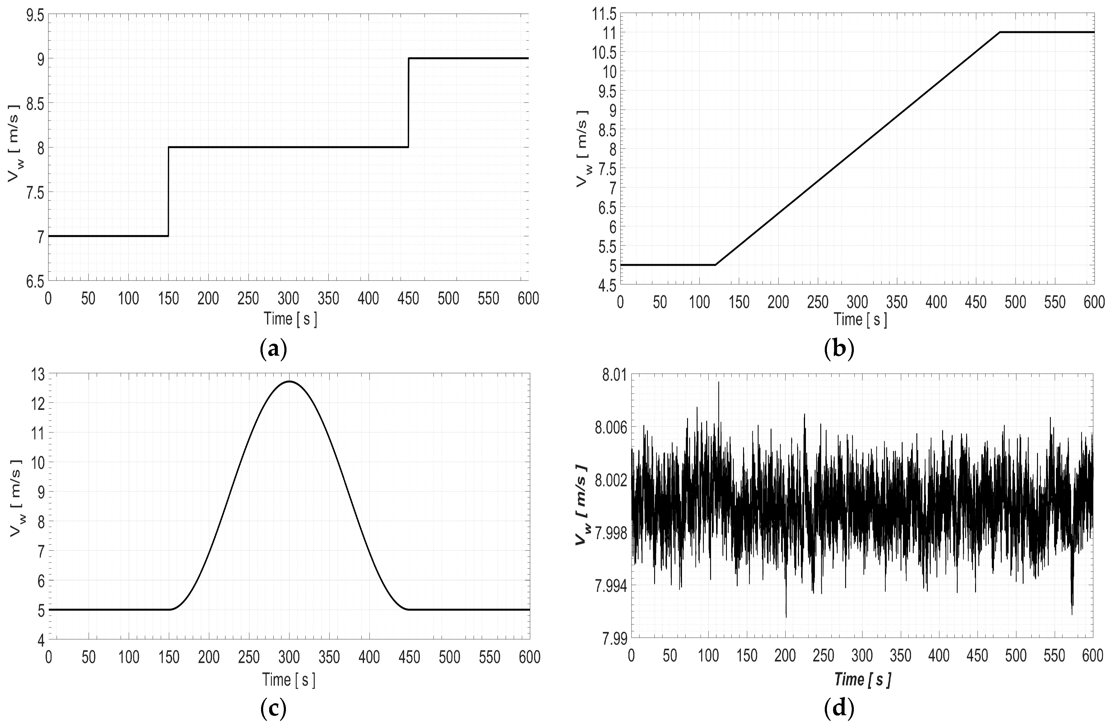
• WSP–A: wind speed profile starts with $7 \mathrm{m}/\mathrm{s},$ maintaining this value for $150 \mathrm{s}$. Then follows an increase in speed of $1 \mathrm{m}/\mathrm{s}$, remaining at this value for $300 \mathrm{s}$. After that, a new increase in speed of 1 m/s is maintained until the end of the simulation. This profile is based on the wind profiles used in [43,48,52,53,54];
• WSP–B: wind speed profile starts at $5 \mathrm{m}/\mathrm{s}$ and maintains that speed for up to $120 \mathrm{s}$. Subsequently, a linear increase in speed begins at 11 m/s over a $360 \mathrm{s}$ interval. After that, the speed value remains at $11 \mathrm{m}/\mathrm{s}$ until the end of the simulation. This profile is based on the wind profiles used in [43,52,60];
• WSP–C: It is a simplified wind gust profile based on the works [52,60,61]. The simplified wind gust profile is given by

  $$V_w\left(t\right)=\{\begin{array}{c}5, t\le T_1\\ 5+V_{gust} \left[1-\cos \left({\displaystyle \frac{2\pi \left(t-T_1\right)}{T_2-T_1}}\right)\right]\\ 5, t>T_2\end{array} T_1<t\le T_2,$$

  (30)

  $V_{gust}=3.85846 \mathrm{m}/\mathrm{s}$ is the amplitude speed of gust, $T_1=150 \mathrm{s}$ is starting time of the gust and $T_2=450 \mathrm{s}$ is end time of gust. We adjusted the value of $V_{gust}$ so that the peak gust velocity would not exceed $V_{rated}$.
• WSP–D: It is a turbulent wind profile given by $V_w\left(t\right)=V_m+V_t$.$V_m$ is the mean value and $V_t$ is the turbulent component [11]. The value of $V_m$ was assumed equal to 8.0 m/s. The turbulent component $V_t$ was obtained by Kaimal turbulence spectra [11,44,46,54,60]. We consider turbulence to be normal based on [62], with ${\sigma }_1$ given by

  $${\sigma }_1=I_{ref} \left(0.75 V_{hub}+5.6\right),$$

  (31)

  $I_{ref}$ equal to 0.18, for class A in [63]. $V_{hub}$ is wind speed at hub height that assumed equal $V_m$ in this work.

Figure 3 shows a graphical representation of the four wind conditions used in this study.

The Q and R matrices used were chosen according to the wind conditions. For WSP–A and WSP–D, the $\mathit{Q}$ and $\mathit{R}$ matrices are:

$$\mathit{Q}={10}^4\left[\begin{array}{cc}1& 0\\ 0& 200\end{array}\right], \mathit{R}=\left[1\right].$$

(32)

Using Equation (22), we obtain the $\mathit{P}$ matrix as

$$\mathit{P}=\left[\begin{array}{cc}4976.624& -97.208\\ -97.208& 1406.149\end{array}\right].$$

(33)

Replacing $\mathit{R},\mathit{B},\mathit{P}$ in Equation (21), results in a signal $u$ equal to:

$$u=97.208 e_1-1406.149 e_2.$$

(34)

The OLFC controller signal is then obtained by $\mathit{U}=\tilde{\mathit{u}}+{\mathit{u}}_f$. The closed-loop poles $\mathit{E}$ of the system are as follows:

$$\mathit{E}=\left[\begin{array}{c}-1.957\\ -1414.248\end{array}\right],$$

(35)

both poles are negative real numbers, as required for the stability of the closed-loop system.

For WSP–B and WSP–C, the $\mathit{Q}$ and $\mathit{R}$ matrices are:

$$\mathit{Q}={10}^4\left[\begin{array}{cc}1& 0\\ 0& 1\end{array}\right], \mathit{R}=\left[0.0001\right].$$

(36)

Solving Equation (22) yields:

$$\mathit{P}=\left[\begin{array}{cc}361.773& -0.998\\ -0.998& 1.002\end{array}\right].$$

(37)

Replacing $\mathit{R},\mathit{B},\mathit{P}$ in Equation (21), we obtain the control $u$ by

$$u=9979.965 e_1-10017.574 e_2.$$

(38)

The closed-loop poles $\mathit{E}$ of the system are as follows:

$$\mathit{E}=\left[\begin{array}{c}-27.663\\ -9999.967\end{array}\right],$$

(39)

both poles are negative real numbers, as required for the stability of the closed-loop system.

We selected the $\mathit{Q}$ matrix for WSP–A and WSP–D to emphasize $T_g$. For WSP–B and WSP–C, we weighted ${\omega }_g$ and $T_g$ equally in the $\mathit{Q}$ matrix. We prioritized reducing control energy by using a low value of $\mathit{R}$.

5. Results and Discussions

The following sections present the results obtained in this study. The analysis and discussion examine the results for each evaluated wind condition. Next, the study presents the annual energy production corresponding to each of these conditions. Finally, the discussion addresses considerations related to the models and the results.

5.1. Results of WSP–A

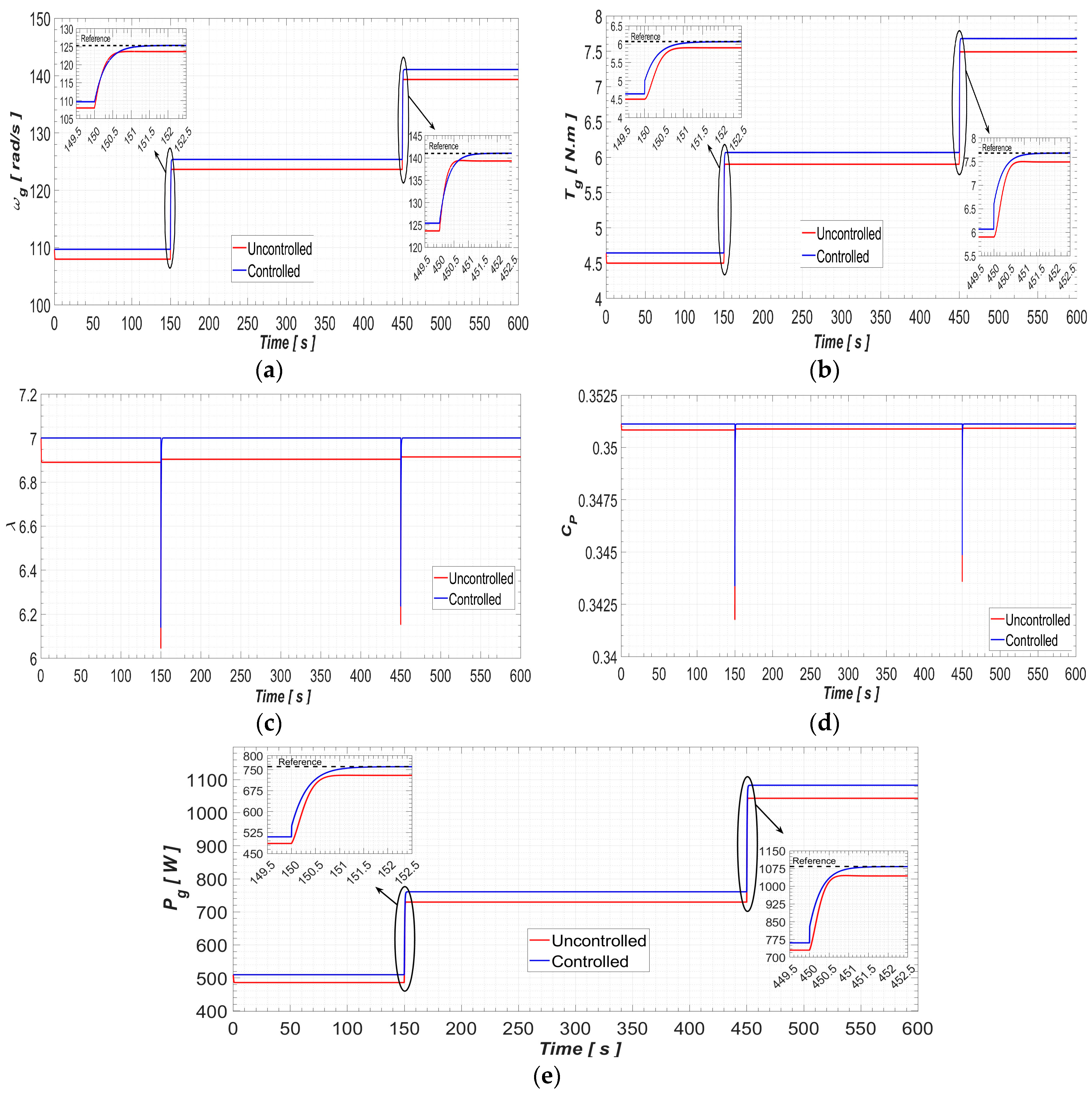
Figure 4 shows the results obtained from the simulation using the WSP–A. In all the graphs of Figure 4, the blue line remains above the red line. This indicates a superior response of the controlled system in all parameters. Figure 4a–c show a clearer difference in the parameters ${\omega }_g$, $T_g$, and $\lambda$. The differences in $C_P$ appear less pronounced. In Figure 4c,d, there is an abrupt variation in both systems in the step speed instants. When analyzing the available $P_g$ in Figure 4e, it is evident that the differences between the systems increase with each change in speed.

We magnified Figure 4a,b,e in the regions corresponding to the step speeds 7–8 m/s and 8–9 m/s. The dashed lines indicate the state reference values following the step speed. Equation (24) yields these values. While their product defines the reference value for $P_g$. For each speed step, we calculated $\mathrm{overshoot}$ and settling time $\left(t_s\right)$ for the controlled system to settle within 2% of the corresponding reference value [28].

Table 1. Results of t_s and overshoot of the variables ${\omega }_g$, $T_g$ and $P_g$ for the controlled system.

Variable	${\mathit{t}}_{\mathit{s}\mathbf{,}\mathbf{7}\mathbf{-}\mathbf{8}}$ [s]	${\mathbf{o}\mathbf{v}\mathbf{e}\mathbf{r}\mathbf{s}\mathbf{h}\mathbf{o}\mathbf{o}\mathbf{t}}_{\mathbf{7}\mathbf{-}\mathbf{8}}$	${\mathit{t}}_{\mathit{s}\mathbf{,}\mathbf{8}\mathbf{-}\mathbf{9}}$ [s]	${\mathbf{\%} \mathbf{o}\mathbf{v}\mathbf{e}\mathbf{r}\mathbf{s}\mathbf{h}\mathbf{o}\mathbf{o}\mathbf{t}}_{\mathbf{8}\mathbf{-}\mathbf{9}}$
${\omega }_g$	$1.845$	0.018	$1.730$	0.022
$T_g$	$1.240$	0.001	$1.185$	0.002
$P_g$	$2.895$	2.300 × 10−5	$2.795$	3.372 × 10−5

presents the obtained $t_s$ and overshoot for the variables ${\omega }_g$, $T_{g,}$ and $P_g$.

The $t_s$ values for variable ${\omega }_g$ rather than those of $T_g$. The result stems from setting $Q_{22}$ higher than $Q_{11}$ in Equation (32). Since both variables drive power dynamics, $P_g$ showed higher settling times. The OLFC can meet the 2% criterion within acceptable timeframes. A tuning value for $Q_{11}$ in Equation (32) can allow faster settling. The overshot values were determined after each step. The overshot values are approximately ${10}^{-2}$ for ${\omega }_g$ and on the order of ${10}^{-3}$ for $T_g$.

Figure 5a–c show the behavior of the error signal for the states, $e_1, e_2$ and the behavior of the functional $L(T$) throughout the simulation for the WSP–A. In Figure 5a,b, details of the behavior of the $e_1$ and $e_2$ errors in the constant velocity regions were included. The $e_1$ shows stable values in order ${10}^{-2}$ far from the abrupt speed transition regions. The $e_2$ show stable values in order ${10}^{-3}$ far from the abrupt speed transition regions. It is observed that significant variations in the moment of the speed change, given by the discontinuity in the speed profile, occur. The $e_1$ exhibits higher peak amplitudes than $e_2$, which suggests significant variation in the generator’s speed. To reduce peak values, we recommend adjusting the controller’s $\mathit{Q}$ matrix values. Note that all values of $L\left(T\right)$ are positive, guaranteeing the optimality condition of the controller.

5.2. Results of WSP–B

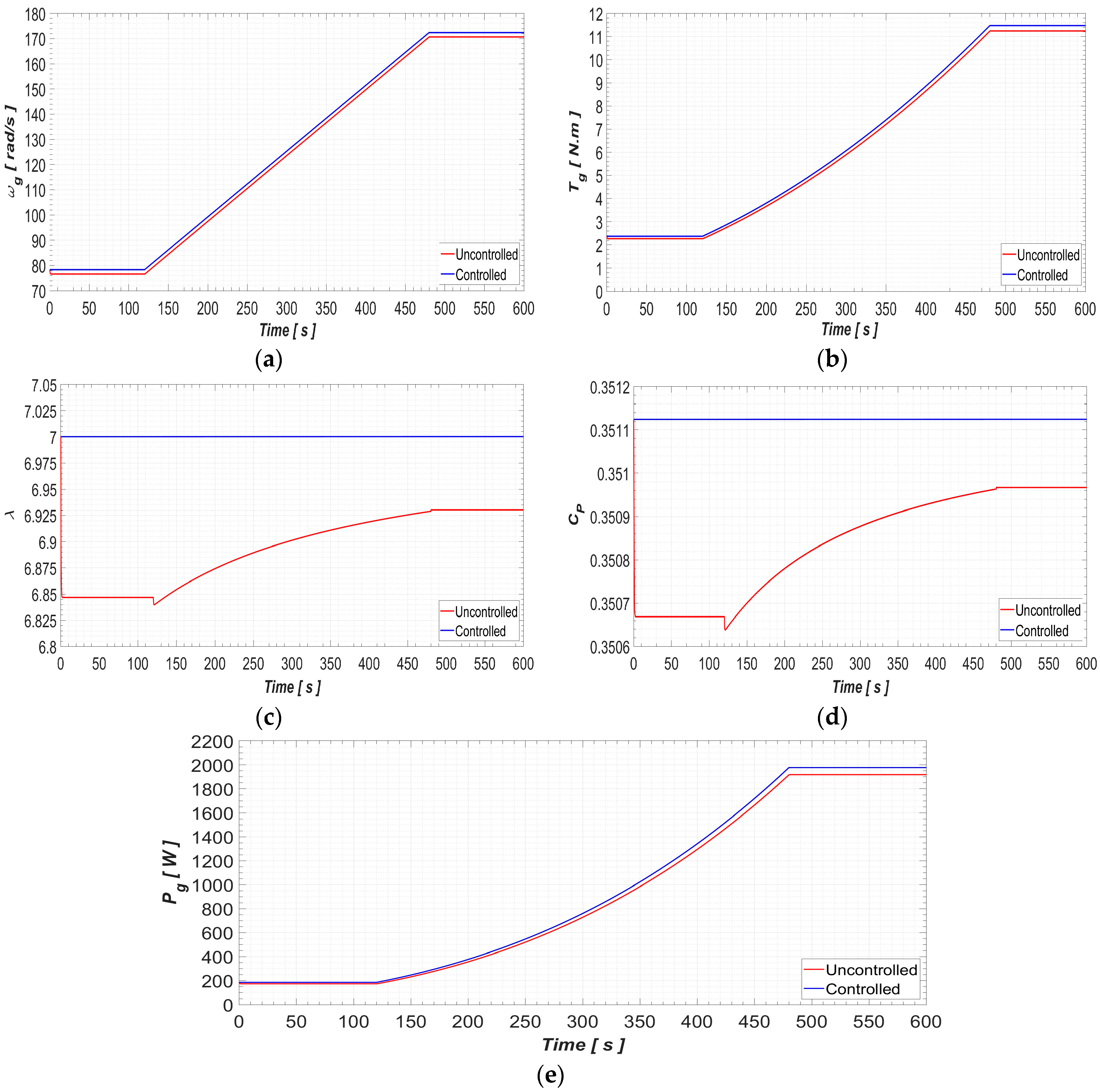
Figure 6 shows the results obtained from the simulation using the WSP–B. As can be seen in Figure 6a,b, the OLFC manages to maintain its ${\omega }_g$ and $T_g$, the values defined by the MPPT strategy at each instant. The wind turbine without control operates suboptimally at all times. The differences in the operation of the uncontrolled and controlled systems become clearer when observing Figure 6c,d. In Figure 6e, between the start of the simulation and around the change in speed, the difference between the systems is minimal. From the start, the linear increase in speed begins. This difference grows until it stabilizes again, reinforcing that the controlled turbine responds more quickly to changes in speed, as previously observed.

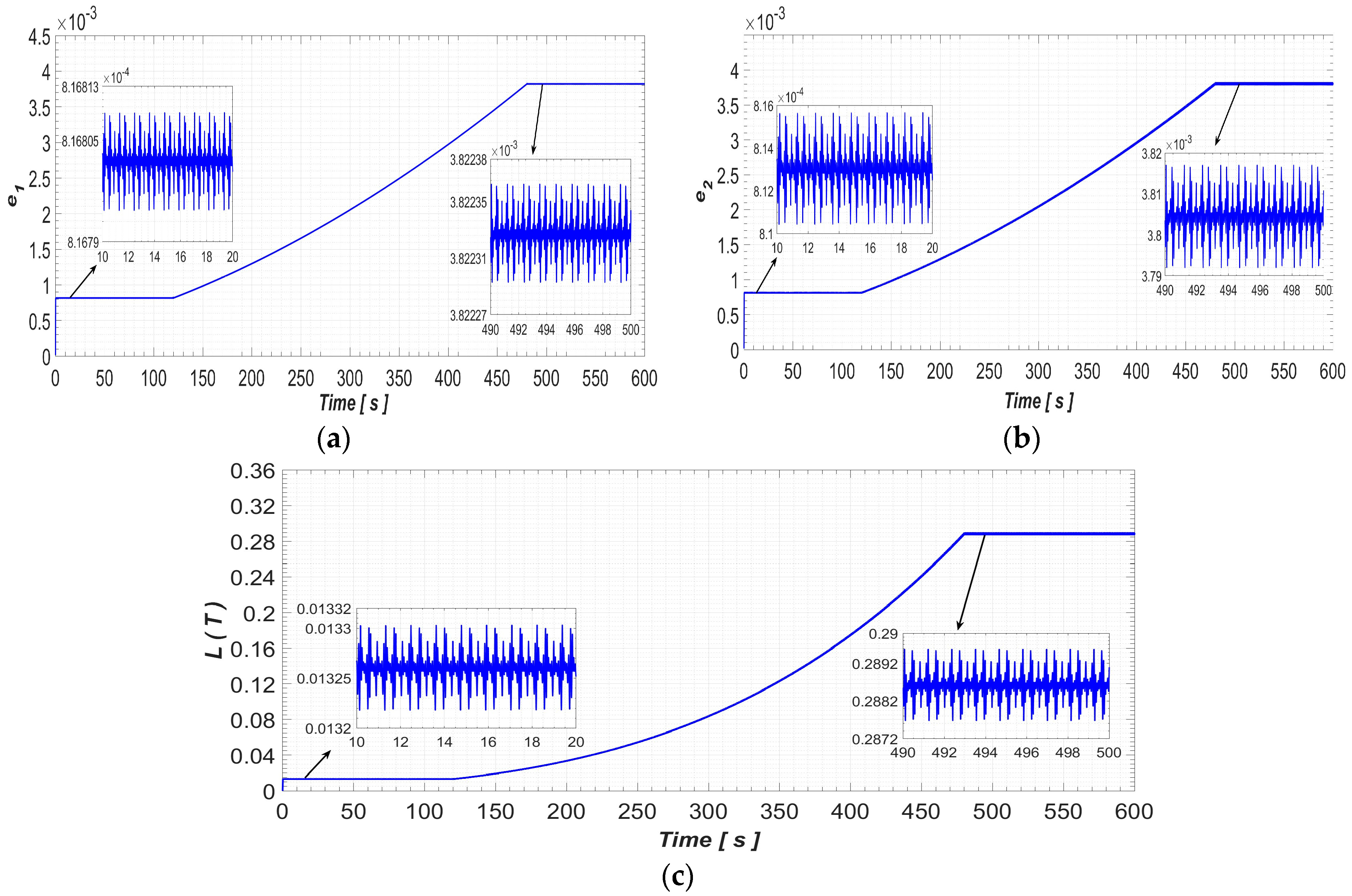
Figure 7a–c show the behavior of the error signal $e_1, e_2$ and the functional $L(T$) throughout the simulation for the WSP–B. The $e_1$ and $e_2$ errors follow the trend of the WSP–B wind profile, since the desired values depend on the wind speed. The magnitudes of $e_1$ and $e_2$ are about ${10}^{-3}$ throughout the simulation time. This indicates the OLFC’s ability to maintain the desired values with acceptable precision and without significant variations. In Figure 7a,b, details of the behavior of the $e_1$ and $e_2$ errors in the constant velocity regions were included. The values found are very similar in magnitude and behavior for $e_1$ and $e_2$. The variations in the flat regions were minor than ${10}^{-3}$. In Figure 7c, the values are positive throughout the simulation. This ensures optimal conditions for the controller. Some oscillations in the flat regions were also observed.

5.3. Results of WSP–C

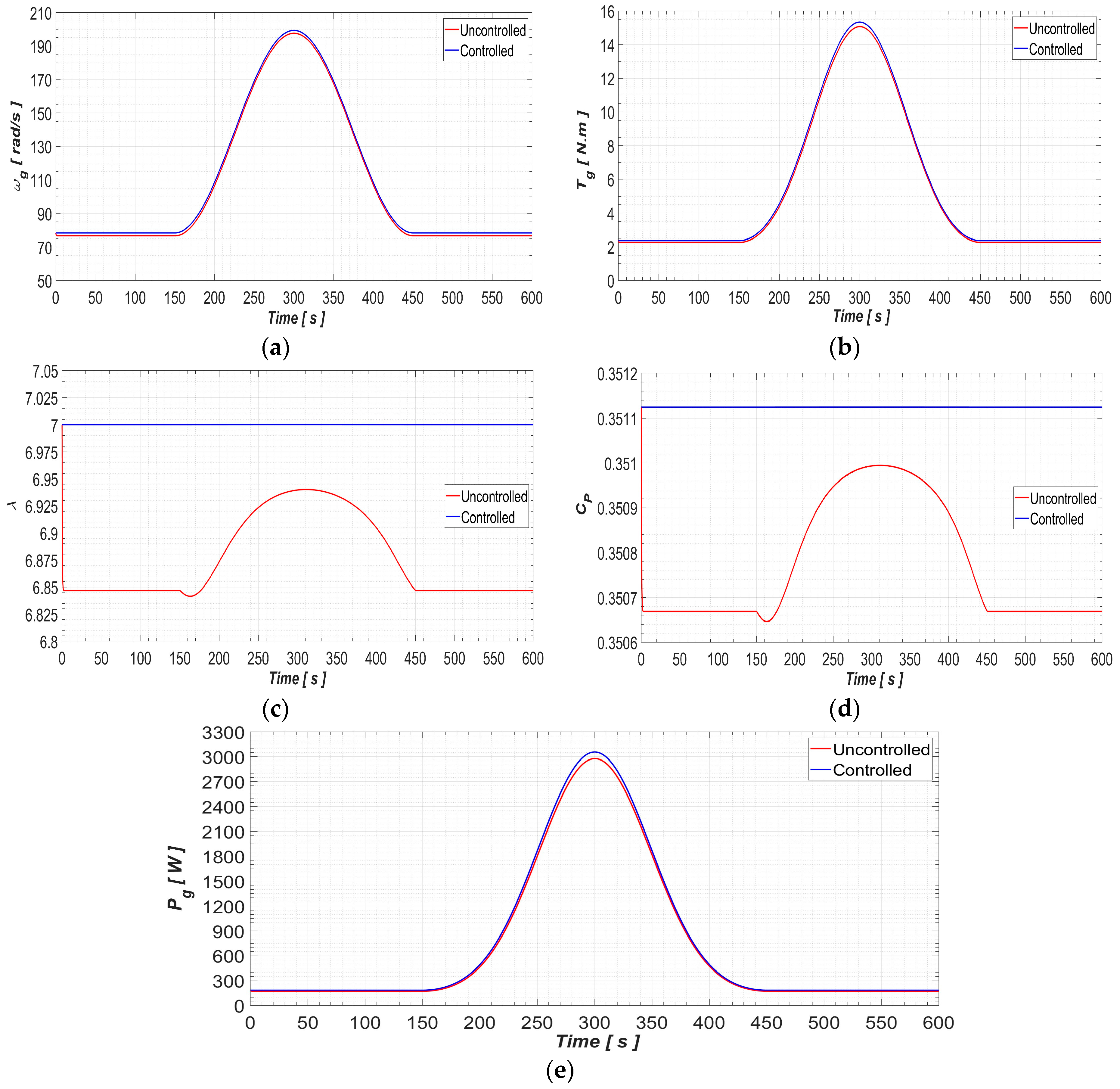
Figure 8 shows the results obtained for the WSP–C. We can see in Figure 8a,b the differences between the systems in the instants before and after the gust are minor. The difference becomes more evident at the gust velocity point. The differences between the systems are more apparent in the aerodynamic parameters $\lambda$ and $C_P$. The controlled system follows the optimal values even during gusts. The uncontrolled system, on the other hand, is more susceptible to variation. This difference is most evident in Figure 8e, which shows that the controlled system extracts more energy during the gust.

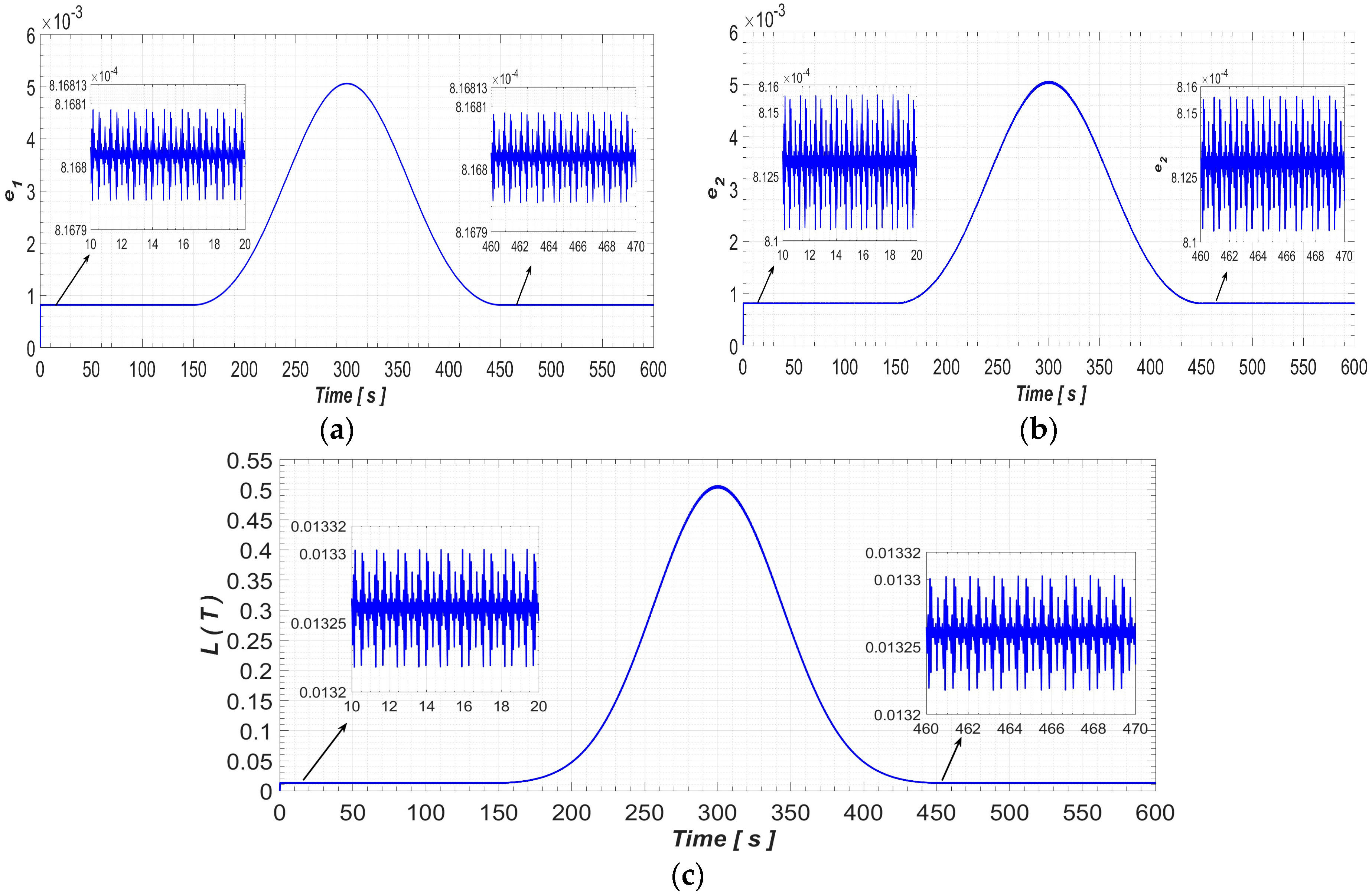
Figure 9a–c show the error signal $e_1, e_2$ and the functional $L(T$) throughout the simulation for the WSP–C. The errors value obtained for the WSP–C profile is similar to that observed in the WSP–B profile. In Figure 9a,b, details in the constant velocity regions were included. The values found are very similar in magnitude and behavior for $e_1$ and $e_2$. The variations in the flat regions were minor than ${10}^{-4}$. Although the speed variation in WSP–C is more complex than that of the WSP–B profile, both profiles exhibit a smooth speed transition. The feedforward component of the controller OLFC works well with this type of variation. In Figure 9c, we see that the values of $L(T$) are positive, indicating that the controller’s optimality conditions are satisfied.

5.4. Results of WSP–D

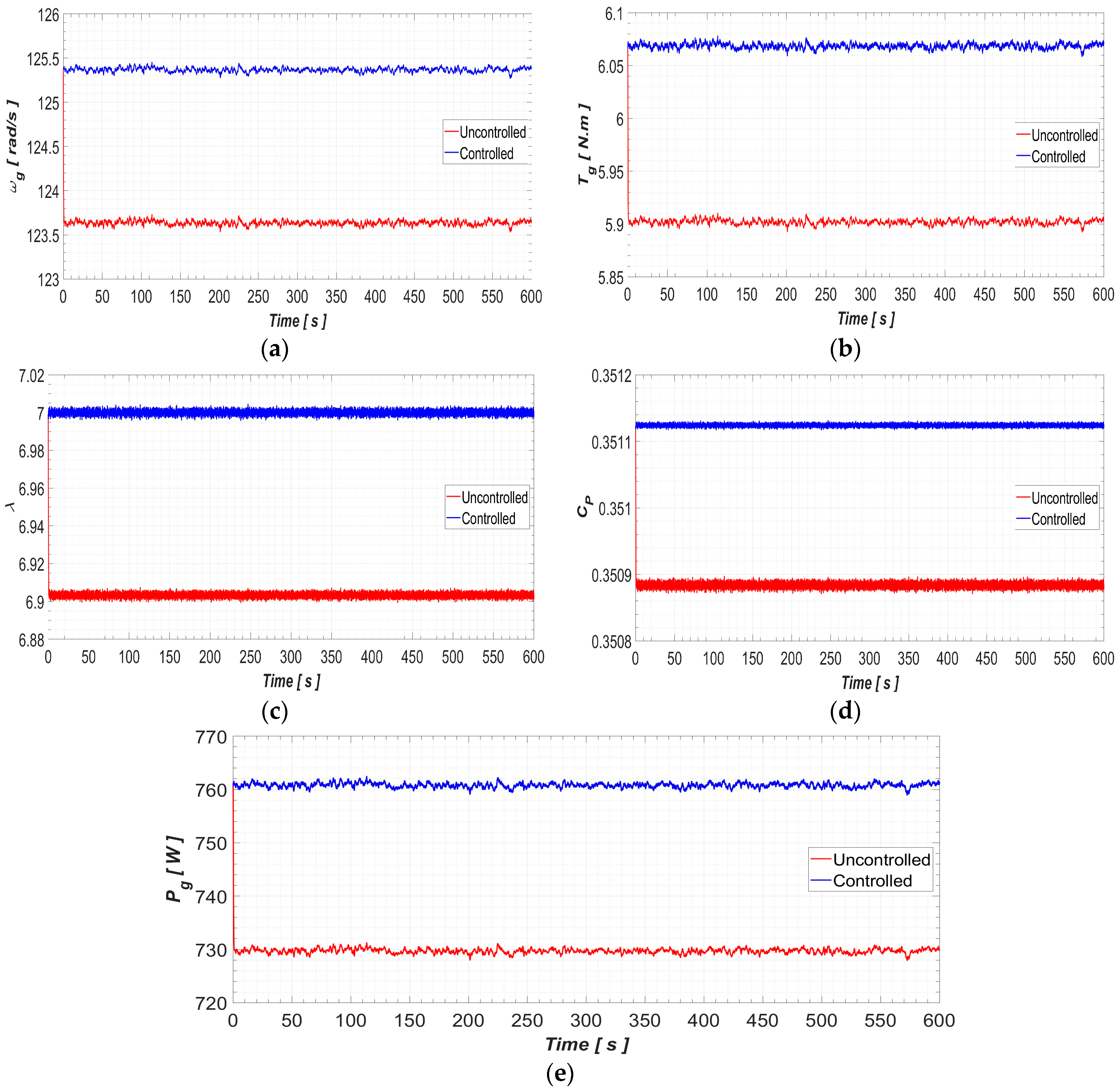
Figure 10 shows the results obtained for the WSP–D. In Figure 10a,b,d,e, the observed behavior for ${\omega }_g$, $T_g$, $C_P$, and $P_g$ is similar. The controlled system exhibits smaller oscillation amplitudes than those observed in the uncontrolled system. Figure 10b shows the behavior of $\lambda$; the oscillations have similar amplitudes in both systems. The values of the parameters analyzed in the controlled system exhibit variations around the MPPT condition. In the uncontrolled system, these oscillations occur around a value that differs from the MPPT condition, resulting in inferior performance.

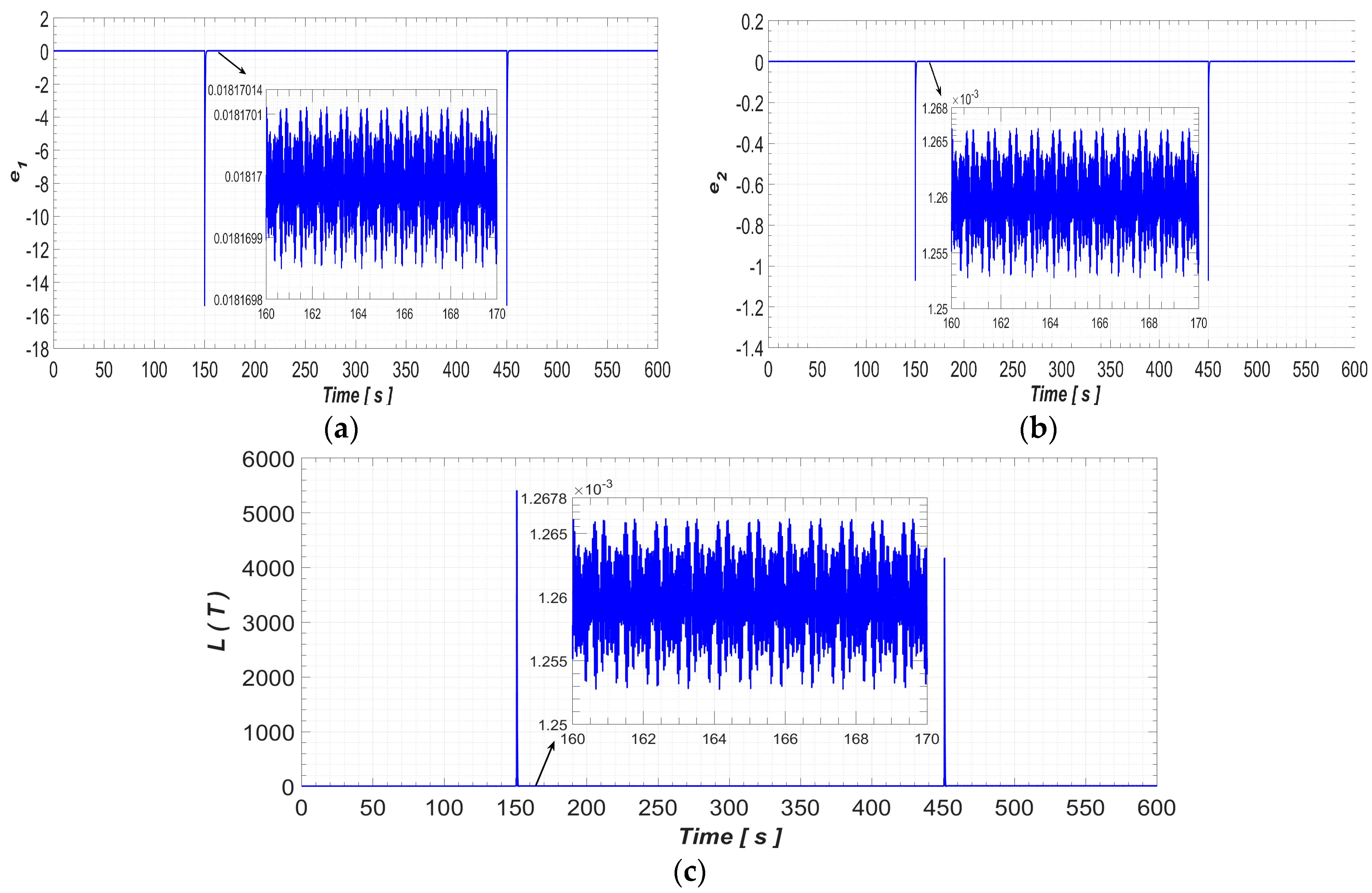
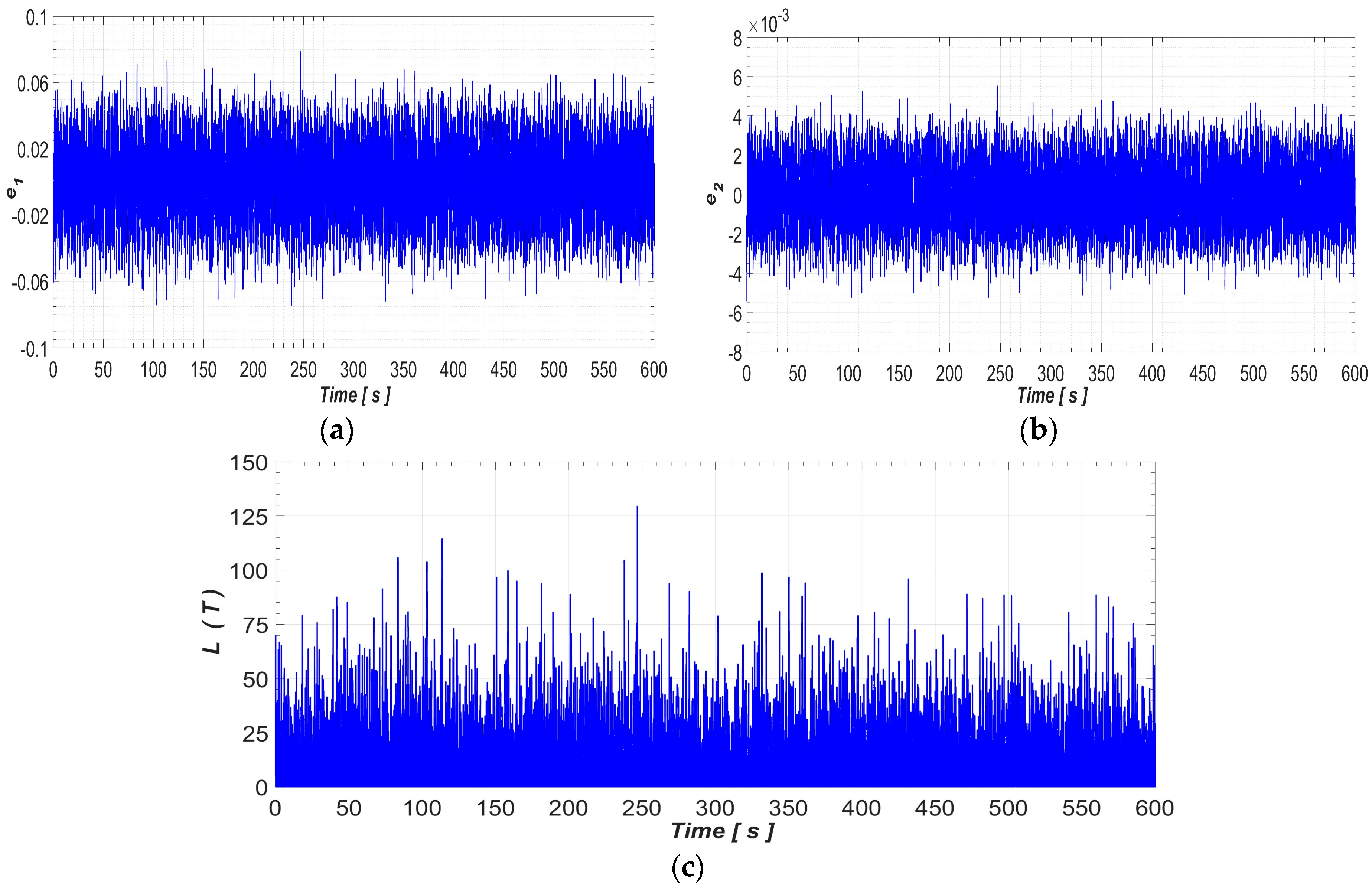
In Figure 11a,b, similar behavior is observed in the temporal variation profile of $e_1$ and $e_2$. However, $e_1$ are an order of magnitude different from the order of magnitude of $e_2$. As observed previously, this is expected, since the matrix $\mathit{Q}$ defined for this condition has a greater weight for $T_g$. The values of $L\left(T\right)$ are all positive, as shown in Figure 11c. This indicates that the OLFC optimality conditions are satisfied.

The results presented for the WSP–D condition are essential to the applicability of the OLFC technique because the WSP–D profile is closer to those found in real-world applications.

5.5. Comparative Analysis of Energy Production

To estimate the impact of behavioral differences between the wind turbine controlled using the OLFC technique and the uncontrolled wind turbine, we calculated the energy generated over the $600 \mathrm{s}$ simulation interval for each wind speed profile. Based on this value, the study estimates the energy generated over one year and presents the results in

Table 2. Energy production for the wind turbine throughout the simulation and the annual energy production estimate.

WSP	Energy in 600 s Uncontrolled [Ws]	Energy in 600 s Controlled [Ws]	Energy in 1 Year Uncontrolled [kWh]	Energy in 1 Year Controlled [kWh]
A	$5.513\times {10}^5$	$5.720\times {10}^5$	$8049.643$	$8351.557$
B	$4.482\times {10}^5$	$4.673\times {10}^5$	$6544.241$	$6821.927$
C	$4.376\times {10}^5$	$4.538\times {10}^5$	$6389.343$	$6625.321$
D	$4.378\times {10}^5$	$4.565\times {10}^5$	$6392.237$	$6664.589$

.

The percentage gain in energy production from the controlled wind turbine compared to the uncontrolled turbine over the course of one year, for each profile, was 3.75%, 4.24%, 3.69%, and 4.26%, respectively.

5.6. Discussions and Limitations

The OLFC controller demonstrated consistent performance and stability across the various wind conditions evaluated. A key advantage of the OLFC method is its use of fixed gains, which ensures implementation complexity comparable to other fixed-gain strategies [30].

In step velocity transitions, such as those observed in the WSP–A profile, temporary disturbances were caused without compromising subsequent system stability, as shown in Table 1.

In smooth velocity transition profiles, such as WSP–B and WS−C, the OLFC controller did not exhibit low-amplitude oscillations. Furthermore, under wind profiles resembling real-world applications with normal turbulence, the controller delivered satisfactory performance, outperforming the uncontrolled system.

The proposed method, integrating OLFC and OT techniques, extracted increased energy from the wind system in all scenarios. While the increase in generated energy is approximately 4%, wind turbines typically possess an expected service life of 20 years. Consequently, this generation gain significantly impacts the cumulative energy yield over the equipment’s entire lifespan.

As previously highlighted, the OT method relies on aerodynamic parameters. Therefore, the turbine’s aerodynamic characteristics directly influence rotational speed and generator torque. Uncertainties regarding these parameters affect both the MPPT strategy’s capabilities and the controller’s performance.

Simplified aerodynamic and mechanical models limit the analyses in this study to small-power wind turbines. Medium- and high-power turbines require high-fidelity models [37]. Therefore, the performance and stability of the OLFC and OT approach when applied to other turbine types may differ from those observed in this work.

6. Conclusions

This work focuses on the application of the OLFC technique in small-scale wind turbines. The results of this study demonstrate that the OLFC controller achieved satisfactory performance when applied to optimal torque (OT) control within the MPPT strategy across different wind speed profiles. Furthermore, the OLFC controller achieved a gain in annual energy production compared to the same uncontrolled wind turbine. The gains were 3.75% (WSP–A), 4.24% (WSP–B), 3.69% (WSP–C), and 4.26% (WSP–D). The main advantage of the OLFC technique lies in its computational simplicity. The OLFC method uses fixed gains, eliminating the need for additional calculations in each iteration.

It is important to note that the conclusions apply only to small-scale turbines. The aerodynamic models used for rotor, shaft, and generator dynamics are simplified. They are not representative of medium and large-scale wind turbines, where flexibility and aerodynamics are influential.

The study suggests the following future possibilities:

• Verification of the OLFC technique’s performance in benchmark models or experimental tests will allow for an understanding of the technique’s strengths and limitations;
• Evaluate the OFC technique associated with the TSR and P&O methods, in applications similar to those in this article;
• Compare the behavior of the OFC technique with other control techniques traditionally used in HAWTs.

References

1. Global Wind Energy Council, GWEC. Global Wind Report 2025. Available online: www.gwec.net/reports/globalwindreport/2025 (accessed on 14 January 2026).
2. Gil-Garcia, I.C.; Fernández-Guillamón, A.; García-Cascales, M.S.; Molina-García, A.; Dagher, H. A green electrical matrix-based model for the energy transition: Maine, USA case example. Energy 2024, 290, 130246. [Google Scholar] [CrossRef] [Scilit]
3. Deghoum, K.; Gherbi, M.T.; Sultan, H.S.; Jameel Al-Tamimi, A.N.; Abed, A.M.; Abdullah, O.I.; Mechakra, H.; Boukhari, A. Optimization of Small Horizontal Axis Wind Turbines Based on Aerodynamic, Steady-State, and Dynamic Analyses. Appl. Syst. Innov. 2023, 6, 33. [Google Scholar] [CrossRef] [Scilit]
4. Borunda, M.; Garduno, R.; de la Cruz Soto, J.; Figueroa Díaz, R.A. Intelligent Control of an Experimental Small-Scale Wind Turbine. Energies 2024, 17, 5656. [Google Scholar] [CrossRef] [Scilit]
5. Olabi, A.G.; Wilberforce, T.; Elsaid, K.; Salameh, T.; Sayed, E.T.; Husain, K.S.; Abdelkareem, M.A. Selection Guidelines for Wind Energy Technologies. Energies 2021, 14, 3244. [Google Scholar] [CrossRef] [Scilit]
6. Pande, J.; Nasikkar, P.; Kotecha, K.; Varadarajan, V. A Review of Maximum Power Point Tracking Algorithms for Wind Energy Conversion Systems. J. Mar. Sci. Eng. 2021, 9, 1187. [Google Scholar] [CrossRef] [Scilit]
7. Dahhani, O.; El-Jouni, A.; Boumhidi, I. Assessment and control of wind turbine by support vector machines. Sust. Energy Tech. Assess. 2018, 27, 167–179. [Google Scholar] [CrossRef] [Scilit]
8. Rajendran, S.; Jena, D.; Diaz, M.; Rodríguez, J. Terminal Integral Synergetic Control for Wind Turbine at Region II Using a Two-Mass Model. Processes 2023, 11, 616. [Google Scholar] [CrossRef] [Scilit]
9. Prajzendanc, P.; Kreischer, C. A Review of New Technologies in the Design and Application of Wind Turbine Generators. Energies 2025, 18, 4082. [Google Scholar] [CrossRef] [Scilit]
10. Idrissi, I.; Chafouk, H.; El Bachtiri, R.; Khanfara, M. Modeling and Simulation of the Variable Speed Wind Turbine Based on a Doubly Fed Induction Generator. In Modeling of Turbomachines for Control and Diagnostic Applications; Loboda, I., Yepifanov, S., Eds.; IntechOpen: London, UK, 2019; Chapter 5. [Google Scholar] [CrossRef] [Scilit]
11. Mérida, J.; Aguilar, L.T.; Dávila, J. Increasing Power Generation Efficiency in Horizontal Wind Turbines by Rejecting Electromechanical Uncertainties Due to the Wind. IEEE Contr. Syst. Lett. 2022, 6, 217–222. [Google Scholar] [CrossRef] [Scilit]
12. Elkodama, A.; Ismaiel, A.; Abdellatif, A.; Shaaban, S.; Yoshida, S.; Rushdi, M.A. Control Methods for Horizontal Axis Wind Turbines (HAWT): State-of-the-Art Review. Energies 2023, 16, 6394. [Google Scholar] [CrossRef] [Scilit]
13. Wang, Q.; Du, Z.; Chen, W.; Ai, C.; Kong, X.; Zhang, J.; Liu, K.; Chen, G. Maximum Power Point Tracking Control of Offshore Hydraulic Wind Turbine Based on Radial Basis Function Neural Network. Energies 2024, 17, 449. [Google Scholar] [CrossRef] [Scilit]
14. Pustina, L.; Biral, F.; Serafini, J. A novel Economic Nonlinear Model Predictive Controller for power maximisation on wind turbines. Renew. Sustain. Energy Rev. 2022, 170, 112964. [Google Scholar] [CrossRef] [Scilit]
15. Saravanakumar, R.; Jena, D. Nonlinear control of wind turbine with optimal power capture and load mitigation. Energy Syst. 2016, 7, 429–448. [Google Scholar] [CrossRef] [Scilit]
16. Qi, L.; Zhao, M.; Wu, S.; Zhang, X.; Meng, P.; Zhao, Y.; Deng, W. Adaptive torque feed-forward control for wind turbine MPPT considering predicted wind speed characteristics. Int. J. Electr. Power Energy Syst. 2025, 167, 110598. [Google Scholar] [CrossRef] [Scilit]
17. He, S.; Wang, B.; Chen, Y. Improved optimal torque control for large scale floating offshore wind turbines based on interval type-2 fuzzy logic system. Ocean. Eng. 2025, 330, 121186. [Google Scholar] [CrossRef] [Scilit]
18. Mazare, M. Adaptive optimal secure wind power generation control for variable speed wind turbine systems via reinforcement learning. Appl. Energy 2024, 353, 122034. [Google Scholar] [CrossRef] [Scilit]
19. Menezes, E.J.N.; Araújo, A.M.; Silva, N.S.B. A review on wind turbine control and its associated methods. J. Clean. Prod. 2018, 174, 945–953. [Google Scholar] [CrossRef] [Scilit]
20. Kumar, D.; Chatterjee, K. A review of conventional and advanced MPPT algorithms for wind energy systems. Renew. Sustain. Energy Rev. 2016, 55, 957–970. [Google Scholar] [CrossRef] [Scilit]
21. Lazzerini, G.; Deleuran Grunnet, J.; Gybel Hovgaard, T.; Caponetti, F.; Datta Madireddi, V.; De Tavernier, D.; Mulders, S.P. COFLEX: A novel set point optimiser and feedforward-feedback control scheme for large, flexible wind turbines. Wind Energy Sci. 2025, 10, 1303–1327. [Google Scholar] [CrossRef] [Scilit]
22. Radaideh, A.; Bodoor, M.; Al-Quraan, A. Active and Reactive Power Control for Wind Turbines Based DFIG Using LQR Controller with Optimal Gain-Scheduling. J. Electr. Comput. Eng. 2021, 2021, 1218236. [Google Scholar] [CrossRef] [Scilit]
23. Mebkhouta, T.; Golea, A.; Boumaraf, R.; Benchouia, T.M.; Karboua, D. A High Robust Optimal Nonlinear Control with MPPT Speed for Wind Energy Conversion System (WECS) Based on Doubly Fed Induction Generator (DFIG). Period. Polytech. Electr. Eng. Comput. Sci. 2024, 68, 1–11. [Google Scholar] [CrossRef] [Scilit]
24. We, H.; Liu, Y.; Lee, S.M.; Park, J.H. Optimal Power Regulating for Wind Turbine with LQR and Disturbance Accommodation Pitch Control. In Proceedings of the 2023 9th International Conference on Control, Automation and Robotics (ICCAR), Beijing, China, 21–23 April 2023; pp. 262–267. Available online: https://ieeexplore.ieee.org/document/10151773 (accessed on 16 February 2026).
25. Rafikov, M.; Balthazar, J.M. On an optimal control design for Rössler system. Phys. Lett. A 2004, 333, 241–245. [Google Scholar] [CrossRef] [Scilit]
26. Rafikov, M.; Balthazar, J.M. On control and synchronization in chaotic and hyperchaotic systems via linear feedback control. Commun. Nonlinear Sci. Numer. Simul. 2008, 13, 1246–1255. [Google Scholar] [CrossRef] [Scilit]
27. Tusset, A.M.; Balthazar, J.M.; Bassinello, D.G.; Pontes, B.R., Jr.; Felix, J.L.P. Statements on chaos control designs, including a fractional order dynamical system, applied to a “MEMS” comb-drive actuator. Nonlinear Dyn. 2012, 69, 1837–1857. [Google Scholar] [CrossRef] [Scilit]
28. Peruzzi, N.J.; Chavarette, F.R.; Balthazar, J.M.; Tusset, A.M.; Perticarrari, A.L.P.M.; Brasil, R.M.F.L. The dynamic behavior of a parametrically excited time-periodic MEMS taking into account parametric erros. J. Vib. Control 2016, 22, 4101–4110. [Google Scholar] [CrossRef] [Scilit]
29. Ribeiro, M.A.; Balthazar, J.M.; Lenz, W.B.; Rocha, R.T.; Tusset, A.M. Numerical Exploratory Analysis of Dynamics and Control of an Atomic Force Microscopy in Tapping Mode with Fractional Order. Shock. Vib. 2020, 2020, 4048307. [Google Scholar] [CrossRef] [Scilit]
30. Daum, H.H.; Tusset, A.M.; Ribeiro, M.A.; Balthazar, J.M.; Bueno, A.M.; Litak, G. Dynamics and Control of a Vibrating System with Hyperchaotic Behavior Using an Electronic Circuit Implementation. Braz. J. Phys. 2022, 52, 104. [Google Scholar] [CrossRef] [Scilit]
31. Ribeiro, M.A.; Balthazarm, J.M.; Daum, H.H.; Tusset, A.M. Dynamical behaviour and Control of a Magnetic structure, composed by a Shape Memory spring driven by a DC motor with limited power supply to harvesting energy. J. Phys. Conf. Ser. 2024, 2647, 252013. [Google Scholar] [CrossRef] [Scilit]
32. Mérida, J.; Aguilar, L.T.; Dávila, J. Analysis and synthesis of sliding mode control for large scale variable speed wind turbine for power optimization. Ren. Energy 2014, 71, 715–728. [Google Scholar] [CrossRef] [Scilit]
33. Mechter, A.; Kemih, K.; Ghanes, M. Backstepping control of a wind turbine for low wind speeds. Nonlinear Dyn. 2016, 84, 2435–2445. [Google Scholar] [CrossRef] [Scilit]
34. Morsi, A.; Abbas, H.S.; Mohamed, A.M. Wind turbine control based on a modified model predictive control scheme for linear parameter-varying systems. IET Control Theory Appl. 2017, 11, 3056–30368. [Google Scholar] [CrossRef] [Scilit]
35. Golnary, F.; Moradi, H. Dynamic modelling and design of various robust sliding mode controls for the wind turbine with estimation of wind speed. Appl. Math. Model. 2019, 65, 566–585. [Google Scholar] [CrossRef] [Scilit]
36. Hassan, A.; Ahmad, G.; Shafiullah, M.; Islam, A.; Shafiul Alam, M. Review of the Intelligent Frameworks for Pitch Angle Control in Wind Turbines. IEEE Access 2025, 13, 29864–29885. [Google Scholar] [CrossRef] [Scilit]
37. Veers, P.; Botasso, C.L.; Manuel, L.; Naughton, J.; Pao, L.; Paquette, J.; Bobertson, A.; Robinson, M.; Anathan, S.; Barlas, T.; et al. Grand challenges in the design, manufacture, and operation of future wind turbine systems. Wind Energ. Sci. 2023, 8, 1071–1131. [Google Scholar] [CrossRef] [Scilit]
38. Li, Z.; Gao, Z.; Chen, Y.; Dai, Y.; Jianwen, W. Unsteady dynamic load and output performance of the rotor using the dynamic wake theory. Energy Sources Part A Recovery Util. Environ. Eff. 2024, 46, 7257–7273. [Google Scholar] [CrossRef] [Scilit]
39. Zhang, H.; Wen, J.; Golnary, F.; Zhou, L. Output Power Control and Load Mitigation of a Horizontal Axis Wind Turbine with a Fully Coupled Aeroelastic Model: Novel Sliding Mode Perspective. Mathematics 2022, 10, 2735. [Google Scholar] [CrossRef] [Scilit]
40. Yang, L.; Liao, K.; Ma, Q.; Khayyer, A.; Sun, H. Coupled aero-servo-elastic method for floating offshore wind turbine wake analysis. Ocean. Eng. 2024, 307, 118108. [Google Scholar] [CrossRef] [Scilit]
41. Brahmi, O.; Bouchema, A.; Kahla, S. New optimal robust control for maximum power point tracking and electromagnetic torque ripple minimization of wind energy conversion system. Wind Eng. 2024, 49, 356–374. [Google Scholar] [CrossRef] [Scilit]
42. El-Baklish, A.K.; El-Badawy, A.A.; Frison, G.; Diehl, M. Nonlinear model predictive pitch control of aero-elastic wind turbine blades. Renew. Energy 2020, 161, 777–791. [Google Scholar] [CrossRef] [Scilit]
43. Sethuraman, L.; Xing, Y.; Gao, Z.; Venugopal, V.; Mueller, M.; Moan, T. A 5MW direct-drive generator for floating spar-buoy wind turbine: Development and analysis of a fully coupled Mechanical model. Proc. Inst. Mech. Eng. Part A J. Power Energy 2014, 228, 718–741. [Google Scholar] [CrossRef] [Scilit]
44. Wen, H.; Liang, D.; Song, Z.; Liu, Y. Adaptive model predictive controller for power regulation and load reduction in large wind turbines. Trans. Inst. Meas. Control 2025, 0. [Google Scholar] [CrossRef] [Scilit]
45. ur Rehman, A.; Ali, N.; Khan, O.; Pervaiz, M. A Disturbance Observer Based Sliding Mode Control for Variable Speed Wind Turbine. IETE J. Res. 2022, 68, 1823–1830. [Google Scholar] [CrossRef] [Scilit]
46. Bouchemal, B.; Chemachema, M. Model-free control for variable-speed wind energy conversion systems based on power tracking. Electr. Eng. 2025, 107, 179–189. [Google Scholar] [CrossRef] [Scilit]
47. Mensou, S.; Essadki, A.; Nasser, T.; Idrissi, B.B.; Tarla, L.B. Dspace DS1104 implementation of a robust nonlinear controller applied for DFIG driven by wind turbine. Renew. Energy 2020, 147, 1759–1771. [Google Scholar] [CrossRef] [Scilit]
48. Sang, Y.; Dai, Z.; Ren, Y.; Wu, Q.; Wang, Y.; Xue, H. NESO-based nonlinear proportional-integral pitch control of the TLP-based floating offshore wind turbine. Energy 2025, 333, 137073. [Google Scholar] [CrossRef] [Scilit]
49. Elbeji, O.; Hannachi, M.; Benhamed, M.; Sbita, L. Artificial neural network–based sensorless control of wind energy conversion system driving a permanent magnet synchronous generator. Wind Eng. 2020, 45, 459–476. [Google Scholar] [CrossRef] [Scilit]
50. Guo, L.; Yin, M.; Cai, C.; Xie, Y.; Zou, Y. Optimal Decreased Torque Gain Control for Maximizing Wind Energy Extraction Under Varying Wind Speed. J. Mod. Power Syst. Clean Energy 2023, 11, 853–862. [Google Scholar] [CrossRef] [Scilit]
51. Rafaat, S.M.; Hussein, R. Power Maximization and Control of Variable-Speed Wind Turbine System Using Extremum Seeking. J. Power Energy Eng. 2018, 6, 51–69. [Google Scholar] [CrossRef]
52. Jiao, X.; Meng, W.; Yang, Q.; Fu, L.; Chen, Q. Adaptive continuous neural pitch angle control for variable-speed wind turbines. Asian J. Control 2019, 21, 1966–1979. [Google Scholar] [CrossRef] [Scilit]
53. Nguyen, P.T.H.; Stüdli, S.; Braslavsky, J.H.; Middleton, R. Lyapunov stability of grid-connected wind turbines with permanent magnet synchronous generator. Eur. J. Control 2022, 65, 100615. [Google Scholar] [CrossRef] [Scilit]
54. Saravanakumar, R.; Jena, D. Validation of an integral sliding mode control for optimal control of a three blade variable speed variable pitch wind turbine. Int. J. Electr. Power Energy Syst. 2015, 69, 421–429. [Google Scholar] [CrossRef] [Scilit]
55. Nayl, T.; Mohammed, M.Q.; Muhamed, S.Q. Modelling design of wind turbine generator. Int. J. Adv. Technol. Eng. Explor. 2022, 9, 2394–7454. [Google Scholar] [CrossRef] [Scilit]
56. Ha, K.; Truong, H.V.A.; Dang, T.D.; Ahn, K.K. Recent Control Technologies for Floating Offshore Wind Energy System: A Review. Int. J. Precis. Eng. Manuf. Green Technol. 2021, 8, 281–301. [Google Scholar] [CrossRef] [Scilit]
57. Apata, O.; Oyedoku, D.T.O. An overview of control techniques for wind turbine systems. Sci. Afr. 2020, 10, e00566. [Google Scholar] [CrossRef] [Scilit]
58. Krafczyk, P. Modélisation et Mise en Oeuvre d’une Chaîne de Production Éolienne à Base de la MADA. Autre. 2013. dumas-01244420. Available online: https://dumas.ccsd.cnrs.fr/dumas-01244420v1 (accessed on 16 February 2026).
59. Tusset, A.M.; Rafikov, M.; Balthazar, J.M. An intelligent controller design for magnetorheological damper based on quarter-car model. J. Vib. Control 2009, 15, 1907–1920. [Google Scholar] [CrossRef] [Scilit]
60. Abrous, A.; Wamkeue, R.; Berkouk, E.M. Modeling and simulation of a wind model using a spectral representation method. In Proceedings of the 2015 3rd International Renewable and Sustainable Energy Conference (IRSEC), Marrakech, Morocco, 10–13 December 2015; pp. 1–6. [Google Scholar] [CrossRef] [Scilit]
61. Länger-Möller, A. Simulation of transient gusts on the NREL 5MW wind turbine using the URANS solver THETA. Wind Energy Sci. 2018, 3, 461–474. [Google Scholar] [CrossRef] [Scilit]
62. Manwell, J.F.; Mcgowan, J.G.; Rogers, A.L. Wind Energy Explained: Theory, Design and Application, 2nd ed.; John Wiley & Sons: West Sussex, UK, 2009; p. 329. [Google Scholar]
63. Bao, D.; Jiang, A.; Li, C.; Shi, Z.; Han, Q.; Luo, Y.; Zhang, S. The Study of Structural Dynamic Response of Wind Turbine Blades under Different Inflow Conditions for the Novel Variable-Pitch Wind Turbine. Energies 2024, 17, 4057. [Google Scholar] [CrossRef] [Scilit]
Figure 1. Schematic components of a typical wind turbine.
Energies 19 01129 g001
Figure 2. Simplified two-mass model.
Energies 19 01129 g002
Figure 3. Wind speed profiles used, (a) WSP–A; (b) WSP–B; (c) WSP–C; (d) WSP–D.
Energies 19 01129 g003
Figure 4. The results of the dynamic behavior of the systems for the condition WSP–A (a) ω g ; (b) Tg; (c) λ; (d) CP; (e) Pg.
Energies 19 01129 g004
Figure 5. OLFC controller performance for WSP–A; (a) e1; (b) e2; (c) L(T).
Energies 19 01129 g005
Figure 6. The results of the dynamic behavior of the systems for the condition WSP–B (a) ω g ; (b) Tg; (c) λ; (d) CP; (e) Pg.
Energies 19 01129 g006
Figure 7. OLFC controller performance for WSP–B; (a) e1; (b) e2; (c) L(T).
Energies 19 01129 g007
Figure 8. The results of the dynamic behavior of the systems for the condition WSP–C (a) ω g ; (b) Tg; (c) λ; (d) CP; (e) Pg.
Energies 19 01129 g008
Figure 9. OLFC controller performance for WSP–C; (a) e1; (b) e2; (c) L(T).
Energies 19 01129 g009
Figure 10. The results of the dynamic behavior the systems for the condition WSP–D (a) ω g ; (b) Tg; (c) λ; (d) CP; (e) Pg.
Energies 19 01129 g010
Figure 11. OLFC controller performance for WSP–D; (a) e1; (b) e2; (c) L(T).
Energies 19 01129 g011