Investigation of Subsurface Current Flow Using an Active Front-End Converter for Through-the-Soil Long-Range Wireless Power Transfer

Abstract

There is a strong demand for buried sensor networks in industries including mining, agriculture, geothermal energy, and oil/gas. However, the integration of these sensors is bottle-necked by the need for electric power which cannot be delivered by conventional means, i.e., cables, photocells, and batteries. To mitigate this bottle-neck, a recent technique was developed that utilizes conduction currents through the soil and subsurface (TTS) to transfer power wirelessly over large distances. The work presented here further investigates changes in conducted power signals as they flow over a 50m radius around a buried TTS Transmitter. An Active Front-End (AFE) converter in tandem with an integrated inverter output is used for creating signals with large spectral densities in order to study attenuation effects throughout the subsurface. The changes in the signals’ spectral content over distance are analyzed and discussed. The abilities to separate attenuation from current spread (divergence) from attenuation due to resistive loss are given, allowing the identification of frequencies best suited for long range power transfer.

1. Introduction

The proliferation of wireless sensor networks has become increasingly vital for monitoring and collecting data in various fields such as agriculture, geothermal energy production, mining, and oil/gas. However, the deployment and maintenance of underground sensor nodes pose significant challenges due to the limited accessibility and the need for reliable and efficient power sources. Traditional methods of supplying power to remote devices rely on cumbersome wiring or finite battery life, which face limitations in scalability and long-term viability. In response to these challenges, wireless power transfer (WPT) in outdoor environments has been a focus of much ongoing research. Several works have demonstrated WPT for powering IoT sensors in natural settings [1,2,3,4]. Many of these WPT methodologies utilize inductive power transfer (IPT) and so require the positioning of coils directly over each other to achieve power transmission. The conductivity of the earth can be a significant challenge in this IPT approach, as eddy currents generated in the conductive soil attenuate the signal with depth, lowering the overall efficiency of the IPT system the deeper it is buried. Other WPT methods have explored the collection of EM space-wave radiation in the High Frequency (HF) to Super High Frequency (SHF) bands for powering large area IoT devices [5,6,7,8,9]. In these approaches, an above-ground transmitter emits energy over a field. Receivers at the surface of the ground collect this energy over a long period of time. Once a state-of-charge threshold is met in each receiver, the sensor circuit is energized, measurements are taken, and the data is re-transmitted back to a base-station. The main challenge in this approach is again the conductivity of the earth, as high frequency radio waves do not penetrate the lossy dielectric of the soil.

To address the challenges of underground sensing, a new technique, known as Through-the-Soil or Through-the-Substrate Wireless Power Transfer (TTS WPT), was recently developed that leverages the conductivity of the earth to transfer power [10]. In this technique, a buried set of electrodes in contact with the earth are energized within an SLF to VLF frequency range. At these frequencies, the earth functions like a conductor, allowing a conduction current to radially emanate from the electrodes and into the surrounding earth. This approach is comparable to a Single Wire Earth Return (SWER) system, which utilizes the soil/subsurface as a return path for long distance power distribution in remote areas [11,12,13]. However, unlike SWER, TTS power transfer removes the above ground, single wire, forward path and replaces it with the top strata of the earth, relying exclusively on earth conduction currents through all subsurface strata for energy transmission.

Presently, the only TTS studies conducted have focused on the power electronics development to extend range and system efficiency [10,14]. Range enhancement requires higher drive currents, and different inverter designs have been proposed for developing higher peak conduction currents for TTS transmission [14]. However, the spectral changes that undergo a conducted power signal when flowing through the soil need further investigation. In particular, since the soil is a lossy dielectric, a certain amount of attenuation is expected. Knowing such parameters could be useful when designing larger-scale TTS systems with improved range/efficiency.

Therefore, this work aims to explore any spectral changes that occur as conduction currents flow outward from a TTS TX. In order to increase the spectral density of the conduction currents, an inverter in tandem with an Active Front-End (AFE) converter is used to drive the TTS TX. A capacitive differentiator is used to modify the square-wave output of the inverter to a pulse. The function of the AFE is to rectify the negative pulses, producing an outward divergent positive pulse train. By using pulses of all the same direction and magnitude, the waveforms become harmonically dense, which drastically accelerates the data collection/analysis as opposed to discretely driving the system at individual frequencies.

The manuscript is organized as follows: a brief background is presented with a differentiation between near-field vs. far-field and how the TTS system is affected by skin-depth and resistance between electrodes. Next, the inverter and AFE rectification topology will be presented in the Materials and Methods (Section 2). A triggering scheme will be explored such that the AFE is operated in a Non-Resonant Zero Voltage/Zero Current Switching (NR-ZVZCS) mode, thereby reducing voltage and current stresses on the AFE from the high intensity, 8 kW peak powers of the inverter. Section 3 will present the measurements of the spectral changes in the waveforms over distance, while Section 4 discusses the analysis of the results. The conclusions and key takeaways are reported in Section 5.

2. Materials and Methods

2.1. TTS Background

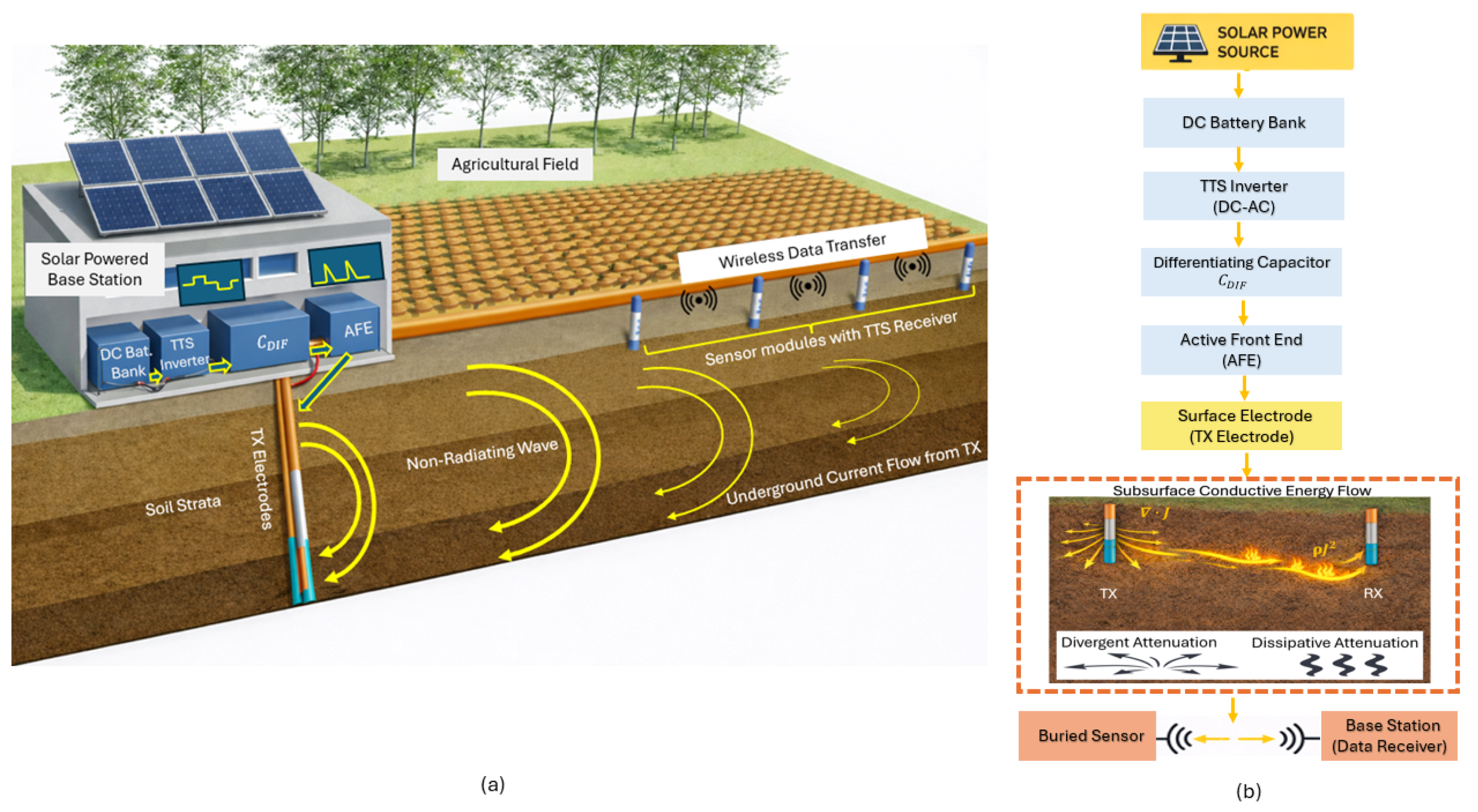
Figure 1 illustrates the proposed Through-the-Soil (TTS) system for agricultural applications, depicting power flow from solar arrays through soil conduction to field receivers and the complete system architecture. Electrical energy harvested from a photovoltaic array charges the DC battery bank and is converted to a high-frequency excitation by a TTS inverter. The signal is shaped by a differentiating capacitor $C_{\mathrm{DIF}}$ and delivered to an Active Front End (AFE), which controls switching and waveform characteristics before coupling the energy into the soil through a surface transmission electrode. The electrode injects an alternating electric field that, due to the conductivity of the soil, produces a current density that travels over and throughout the subsurface, enabling energy transfer through the soil medium. The conducted power signal experiences geometric spreading due to current density divergence $(\nabla ·\mathbf{J})$ and dissipative attenuation from ohmic heating $\rho J^2$. Buried receiver electrodes intercept the subsurface current to power subsurface sensor modules. Power delivery occurs through this conduction current mechanism, while sensed data return to the base station either via the same conduction current methodology, or through conventional wireless RF transmitters (if near the surface). Since there exists very limited research literature on the attenuation factors of near-field excitations within the earth’s subsurface, this work focuses on the frequency spectrum analysis of the subsurface conductive energy flow highlighted in Figure 1b.

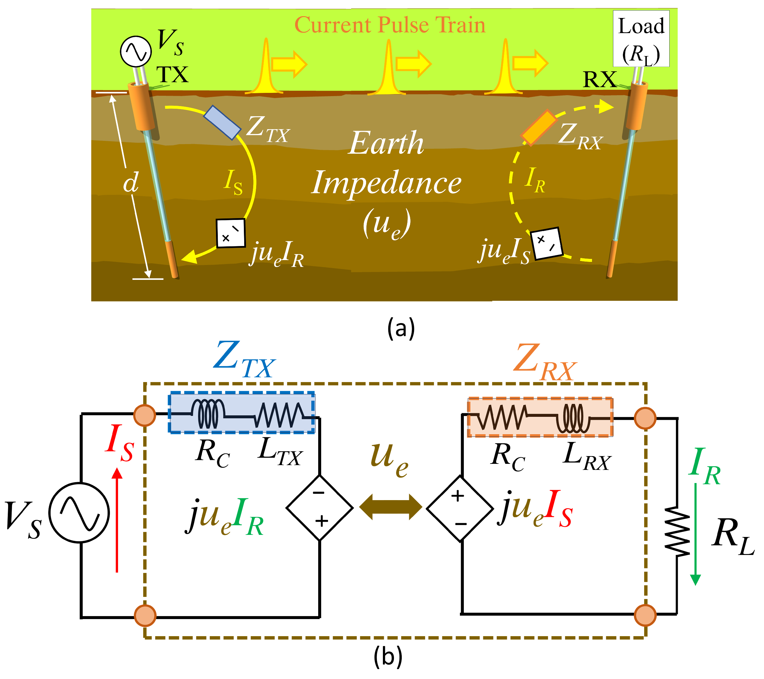
While the TTS system was presented and derived in [10], we will present a brief review of it here. Referring to Figure 2, the TTS transmitter (Tx), in its simplest form, consists of at least two conductors in direct contact with the soil. One electrode is positioned at the soil surface, while the other is placed vertically below the surface. When an alternating voltage is applied to the electrodes, a current is generated throughout the soil which diverges outward in a circular pattern underground. Current flow through the soil is not a new concept. Over the last 2 centuries, current flow from a buried electrode has been extensively studied in power distribution systems for substation grounding [15,16,17,18,19]. Conducted currents are also studied extensively in geophysics, where electrical signals are used to form maps of underground subsurface resistivity [16,20,21,22].

In [10], instead of attempting to electrically model the complex impedance network of the soil around the TX, which is very heterogeneous and highly variable, electromagnetic field theory was employed instead. A Hertzian dipole approximation was used due to the size and separation of the electrodes being significantly small compared to the wavelengths of the frequencies used to excite the TX, which were in the SLF to VLF range (30 Hz to 30 kHz). Readers may recall, a Herztian dipole assumes an infinitesimally small antenna dimension ($dl$) with a uniform current along the structure. This should not be confused with a radiating dipole (half-wave, quarter-wave, etc.), whose physical dimensions are comparable to the wavelengths of frequencies used. For the TTS system driven at SLF-VLF frequencies, the associated wavelengths are between 10,000 km to 10 km. Even if the relative permittivity of the soil was somehow as high as pure water (80), this would still correspond to a wavelength range of 1120 km to 1.1 km, which is far larger than the biggest dimension of the TTS TX (being at most 0.09 km and well below $1/10$ the wavelength). These factors make the Hertzian dipole a decent approximation for deriving TTS field distributions.

Due to Hertzian dipoles being so electrically small, they possess a very low radiation resistance, and thus are very poor far-field radiators. This means that the operational methodology presented in [10] for creating TTS power transfer is, by definition, a system that functions entirely within the near-field. A benefit with a near-field system is that the input impedance is complex, and the power injected into the system does not need to be purely real.

The potential distribution ${\varphi }_e$ around the top electrode was modeled in [10] as

$$\mathfrak{Im}\left\{{\Phi }_e\right\}=\mathfrak{Im}\left\{{\displaystyle \frac{I_{S}d\cos \theta }{4\pi \left({\sigma }^2+{\left(\omega \epsilon \right)}^2\right)}}\left[\left({\displaystyle \frac{\omega \epsilon \beta }{r}}+{\displaystyle \frac{\sigma }{r^2}}\right)-j\left({\displaystyle \frac{\sigma \beta }{r}}+{\displaystyle \frac{\omega \epsilon }{r^2}}\right)\right]\right\}$$

$${\Phi }_e=-{\displaystyle \frac{I_{S}d}{4\pi \left({\sigma }^2+{\left(\omega \epsilon \right)}^2\right)}}\left({\displaystyle \frac{\sigma \beta }{\left(r\right)}}+{\displaystyle \frac{\omega \epsilon }{{\left(r\right)}^2}}\right)$$

(1)

where $I_s$ is the injected current from the source, $\sigma$ is the soil conductivity, $ϵ$ is the soil permittivity, $\omega$ is the angular frequency, and d is the separation distance between top and bottom electrodes. Note that $d=2\pi a$, which takes into account that the separation distance between the electrodes is not just the metal electrodes but also a portion of the soil surrounding the electrodes. From (1), the “earth” impedance ($u_e$) that the underground current encounters as it flows radially (r) outward from the top electrode is defined as

$$u_e=-{\displaystyle \frac{d}{4\pi ({\sigma }^2+{\left(\omega ϵ\right)}^2)}}\left({\displaystyle \frac{\sigma \beta }{\left(r\right)}}+{\displaystyle \frac{\omega ϵ}{{\left(r\right)}^2}}\right)$$

(2)

Equation (2) can be re-written in terms of the loss tangent $(\sigma /\omega \epsilon )$ of the soil/subsurface as

$$u_e=-{\displaystyle \frac{d}{4\pi \omega \epsilon \left({\left(\frac{\sigma }{\omega \epsilon }\right)}^2+1\right)}}\left(\left({\displaystyle \frac{\sigma }{\omega \epsilon }}\right){\displaystyle \frac{\beta }{\left(r\right)}}+{\displaystyle \frac{1}{{\left(r\right)}^2}}\right)$$

(3)

In the SLF/VLF range, ${(\sigma /\omega \epsilon )}^2\gg 1$, such that (3) can be approximated as

$$u_e\approx -{\displaystyle \frac{d\rho }{4\pi }}\left({\displaystyle \frac{\omega n}{c\left(r\right)}}+{\displaystyle \frac{\omega \epsilon \rho }{{\left(r\right)}^2}}\right)$$

(4)

where $\rho$ is the resistivity of the subsurface $(\rho =1/\sigma )$, c is the speed of light in a vacuum, and n is the refractive index of the medium $(n=\sqrt{{\epsilon }_r}$, where ${\epsilon }_r$ is the relative permittivity). It can be seen in (4) that as the frequency is increased, the earth impedance will likewise increase—indicating that the earth’s impedance is similar to an inductance, which will function as a low-pass filter. Normally, inductance is defined as a positive reactance, but this nomenclature comes from making the driving voltage source’s temporal phase the reference point in the circuit. In the derivation of (2), it is the current that is the reference, as the magnetic vector potential of the Hertzian dipole is with respect to the drive current, which is assumed to have zero temporal phase. This flips the sign of the reactance.

The potential distribution over an area around the TTS Tx will increase according to (1) as $u_e$ increases. Higher drive frequency should therefore enhance the potential distribution over the area. However, it should be noted that the source must be restricted to a sufficiently low frequency (VLF, SLF) in order for the approximation of (1) to be valid. The experimental frequency limit determined in [10] was approximately 20 kHz. However, a more detailed investigation of this limit must be conducted.

The real component $R_{TX}$ is defined in the well-known grounding literature [15,16,17,18,19] for the resistance between a pair of buried electrodes in contact with the soil. Ref. [23] splits the total electrode resistance ($R_t$) into a local contact resistance ($R_c$), and a separation resistance ($R_s$). When the electrodes are touching, it is assumed the resistance between the pair is nearly zero ($R_c=R_s$), and as they are separated $R_t$ becomes

$$R_t=R_c-R_s$$

$$R_t={\displaystyle \frac{\rho }{2\pi r_e}}-{\displaystyle \frac{\rho }{2\pi r_s}}$$

(5)

where $\rho$ is the soil resistivity, $r_e$ is the radius of the electrodes (assuming both electrodes have the same radius) which is fixed, and $r_s$ is the separation distance between electrodes. For a TTS TX with an electrode separation of 90 m and a soil resistivity of 200 Ωm, $R_s$ is only 0.35 Ω. The majority of the loss is thus from the contact resistance ($R_c$) which can be lowered by using multiple ground rods [15,16,17,18,19]. It is important to study how power signals traverse the region surrounding the TTS TX. Knowing the frequencies that attenuate quickly will allow a designer to avoid operating the system at such frequencies. This is also important for the advancement of in-tandem communications, where recent work has focused on utilizing TTS principles to send information completely underground [24].

2.2. Experimental System

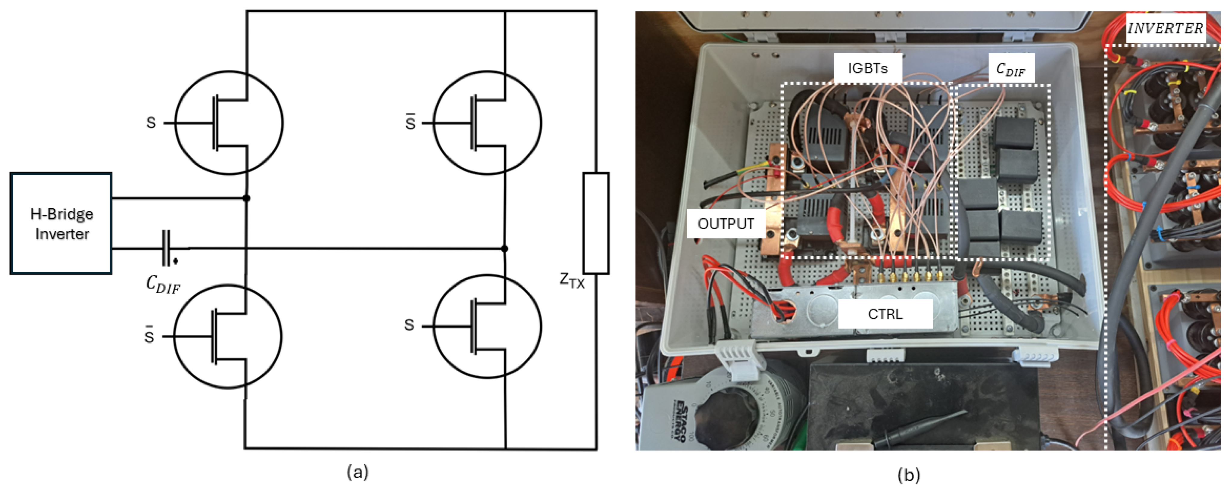
In order to study the effects of frequency on current flowing around a TTS system, the inverter used in [10] was modified with an Active Front End (AFE) converter. The schematic of the experimental system is shown in Figure 3. The approach was to use a capacitance ($C_{DIF}$) in series with the TX input impedance ($Z_{TX}$) that differentiates the square-wave output of the inverter into pulses, all while maintaining large peak current across $Z_{TX}$ so that the TTS signal range over the soil/subsurface was maximized. The AFE circuit topology is shown in Figure 3, which is comprised of an H-bridge converter configuration fed by an H-bridge inverter. The differentiation capacitor $\left(C_{DIF}\right)$ was placed in series with the inverter. $C_{DIF}$ and the impedance of the TTS TX form a low-pass filter with a time constant ($\tau$). As long as the inverter switching speed was much lower than this $\tau$, a current pulse would flow through $Z_{TX}$ during the inverter’s first half cycle, while a negative current pulse would flow in the inverter’s second half cycle. Changing the value of $C_{DIF}$ would change the width of the current pulse across $Z_{TX}$.

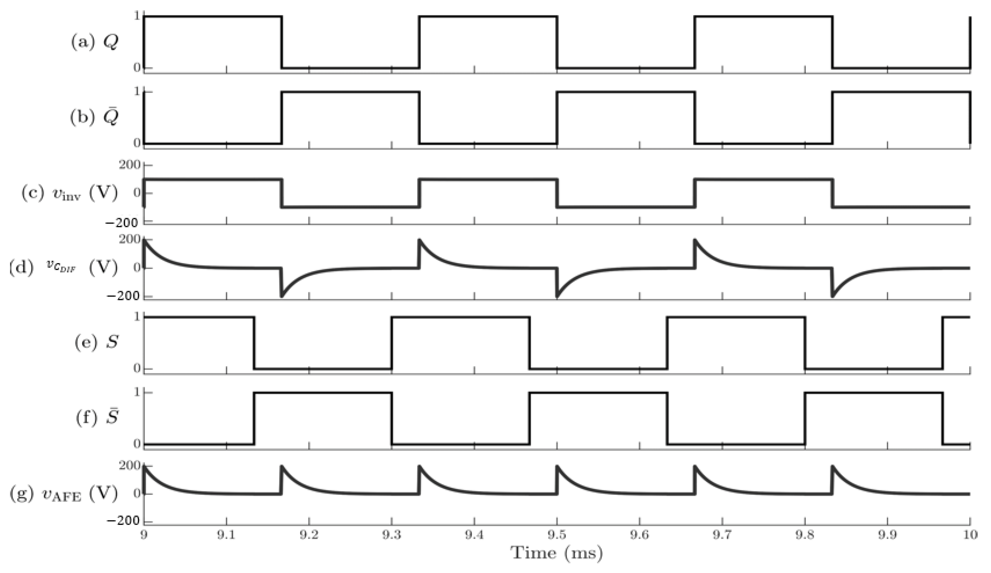
The inverter operated at a 50% duty cycle square-wave at a frequency of 500 Hz. Proper timing of the AFE allowed the negative pulses of the differentiated inverter output to be rectified. This created a continuous positive pulse train at twice the inverter’s switching frequency (1 kHz). If the AFE was triggered during time periods where the voltage and current across the load were significantly low, a ZVZC switching would be achieved and very little stress would be placed on the AFE transistors. The timing diagram of the AFE switching waveforms are shown in Figure 4 along side the resulting output waveform that entered the TTS TX. The switching signals represented by Q and $\overline{Q}$ represent the on state with a logic 1 (Q) and off state with a logic zero ($\overline{Q}$) of the inverter, while the S and $\overline{S}$ represent those of the AFE.

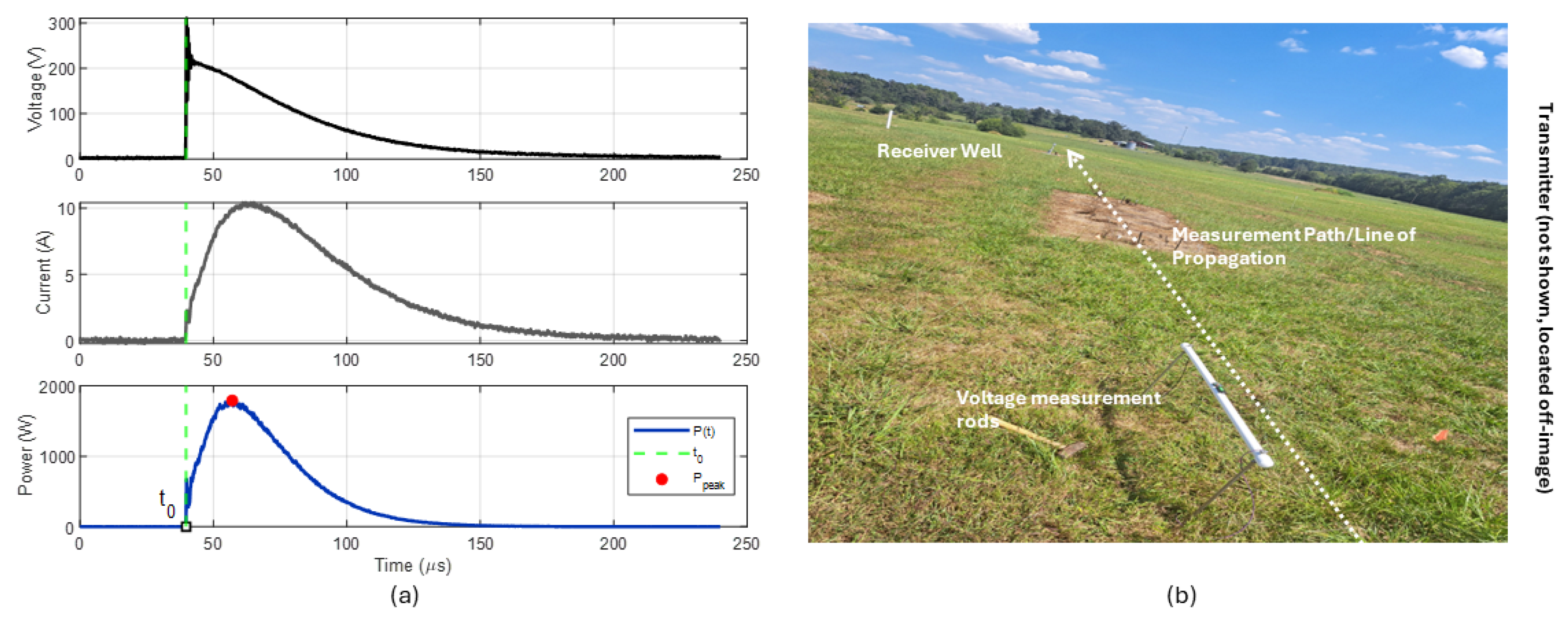
Figure 5a shows the measured voltage, current, and instantenous power waveforms of a single pulse within the pulse train that were output from the AFE and injected into the TTS TX. Note that there is a phase shift between the voltage and current pulses measured across $Z_{TX}$, which demonstrates that the TX input impedance has a reactive component. This is a rather unique result, since potentials throughout the subsurface are in phase with the injected current; the phase difference manifests between the voltage source and the currents throughout the ground, indicating that the earth (not just the metal structure of the TX) acts partly as an inductor. The potential difference created by the current flowing over the area was measured using the same technique shown in [10] and annotated in Figure 5b. The pulse train was captured at 10 distinct locations between 1 m spaced receiving electrodes.

3. Closed-Form Average Pulse Power Approximation

It would be advantageous to calculate the average pulse power from an equation that utilizes the peak power measurements without having to record the pulse train, multiply the signals together, and then integrate over the period. With this in mind, the following is a derivation of a few approximate equations that allow quick calculation based on basic oscilloscope measurements, without either relying on the math function of the scope (which may not always be available) or data collection and processing.

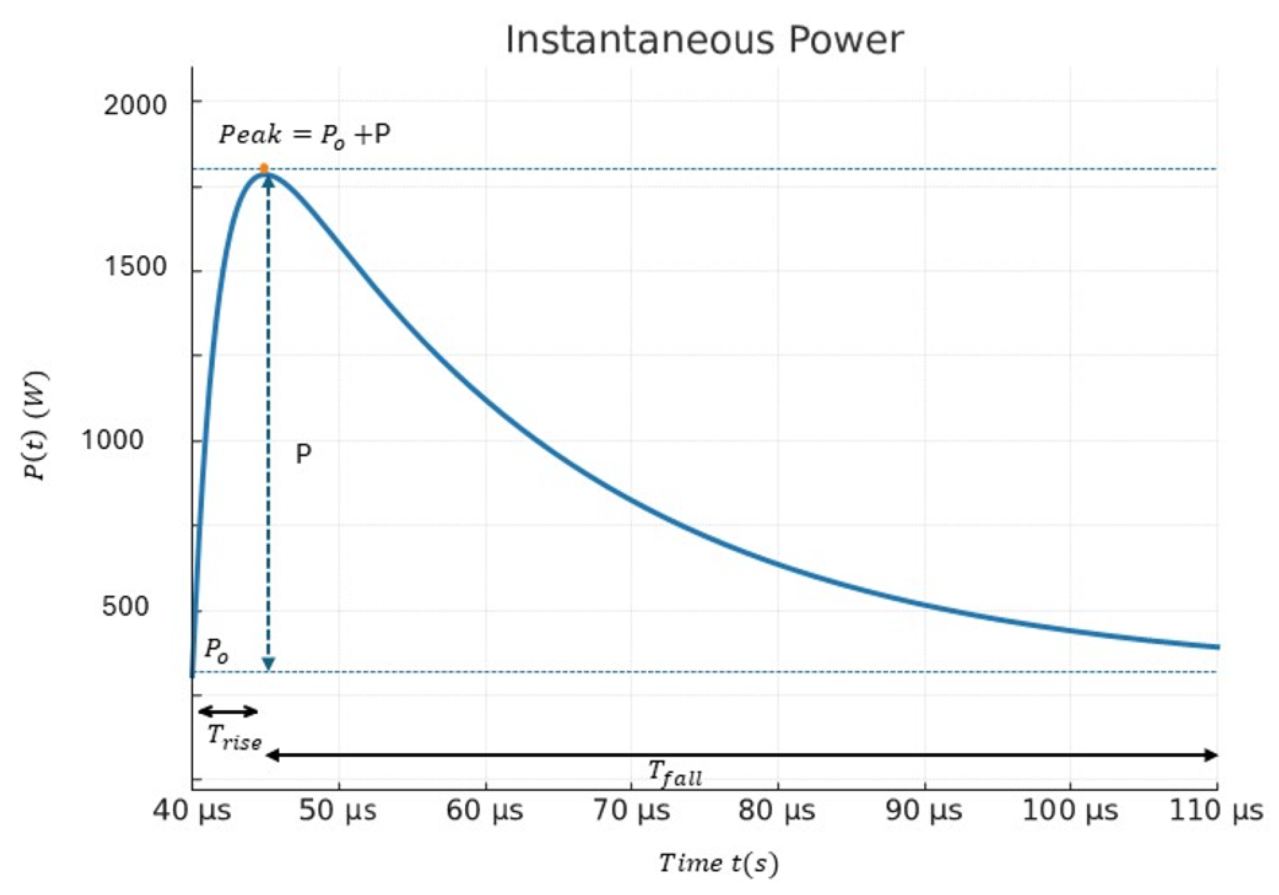
To do this we must first approximate the shape of the resulting instantaneous waveform of Figure 5. This approximate waveform is shown in Figure 6. The instantaneous power will thus be

$$P\left(t\right)=v_{\mathrm{well}}\left(t\right)i_{\mathrm{well}}\left(t\right),$$

and is modeled over the window $[t_0,t_0+T]$ by a half-sine rise followed by a half-sine fall, with $T=T_{\mathrm{rise}}+T_{\mathrm{fall}}$:

$$P\left(t\right)=\left\{\begin{array}{cc}{P}_0+P\sin \left({\displaystyle \frac{\pi (t-t_0)}{2T_{\mathrm{rise}}}}\right),\hfill & t_0\le t<t_0+T_{\mathrm{rise}},\hfill \\ P_0+P\sin \left({\displaystyle \frac{\pi (t_0+T_{\mathrm{rise}}+T_{\mathrm{fall}}-t)}{2T_{\mathrm{fall}}}}\right),\hfill & t_0+T_{\mathrm{rise}}\le t\le t_0+T_{\mathrm{rise}}+T_{\mathrm{fall}}.\hfill \end{array}\right.$$

(6)

Here $P_0=P\left(t_0\right)$ is the baseline and $P=P_{\mathrm{peak}}-P_0$ is the incremental peak above baseline. By construction,

$$P\left(t_0\right)=P(t_0+T)=P_0,P\left(t_0+T_{\mathrm{rise}}\right)=P_0+P.$$

(7)

Full-width-at-half-maximum (FWHM).

Let $P_{1/2}=P_0+\frac{P}{2}$. Solving $P\left(t\right)=P_{1/2}$ for the rising and falling edges yields

$$t_1=t_0+{\displaystyle \frac{T_{\mathrm{rise}}}{3}},t_2=t_0+T_{\mathrm{rise}}+{\displaystyle \frac{2T_{\mathrm{fall}}}{3}},$$

(8)

so the FWHM is

$$\mathrm{PW}=t_2-t_1={\displaystyle \frac{2}{3}}\left(T_{\mathrm{rise}}+T_{\mathrm{fall}}\right)={\displaystyle \frac{2}{3}}T.$$

(9)

Average over the pulse window $[t_0,t_0+T]$.

$$\overline{P}={\displaystyle \frac{1}{T}}{\int }_{t_0}^{t_0+T}P\left(t\right)dt={\displaystyle \frac{1}{T}}\left(I_{\mathrm{rise}}+I_{\mathrm{fall}}\right),$$

(10)

with the normalized changes of variables

$$u={\displaystyle \frac{t-t_0}{T_{\mathrm{rise}}}}\in [0,1],v={\displaystyle \frac{t_0+T-t}{T_{\mathrm{fall}}}}\in [0,1].$$

(11)

This gives

$$\begin{array}{cc}\hfill I_{\mathrm{rise}}& =P_0{T}_{\mathrm{rise}}+P{T}_{\mathrm{rise}}{\int }_0^1\sin \left({\displaystyle \frac{\pi u}{2}}\right)du=P_0{T}_{\mathrm{rise}}+{\displaystyle \frac{2}{\pi }}P{T}_{\mathrm{rise}},\hfill \end{array}$$

(12)

$$\begin{array}{cc}\hfill I_{\mathrm{fall}}& =P_0{T}_{\mathrm{fall}}+P{T}_{\mathrm{fall}}{\int }_0^1\sin \left({\displaystyle \frac{\pi v}{2}}\right)dv=P_0{T}_{\mathrm{fall}}+{\displaystyle \frac{2}{\pi }}P{T}_{\mathrm{fall}}.\hfill \end{array}$$

(13)

Therefore,

$$\begin{array}{|c|}\hline \overline{P}=P_0+{\displaystyle \frac{2}{\pi }}P=P_0+{\displaystyle \frac{2}{\pi }}\left(P_{\mathrm{peak}}-P_0\right).\\ \hline\end{array}$$

(14)

For the half-sine model, $\overline{P}$ is independent of $T_{\mathrm{rise}}$ and $T_{\mathrm{fall}}$.

Figure 6. Instantaneous power waveform and timing definitions.

Figure 6. Instantaneous power waveform and timing definitions.

Complementary Averages for Periodic Excitation

Each expression below is closed-form and depends only on $P_0,P_{\mathrm{peak}}$ (or their FWHM equivalent).

• Per-pulse average (pulse window only):

  $${\overline{P}}_{\mathrm{pulse}}=P_0+{\displaystyle \frac{2}{\pi }}P=P_0+{\displaystyle \frac{2}{\pi }}\left(P_{\mathrm{peak}}-P_0\right).$$

  (15)
• Period average with true duty (repetition every $1/f$ s, baseline $P_0$ between pulses):

  $${\overline{P}}_{\mathrm{period}}=P_0+{\displaystyle \frac{2}{\pi }}P\delta ,\delta \equiv Tf(\mathrm{true}\mathrm{duty}\mathrm{factor}).$$

  (16)
• Period average using FWHM-based duty. For a half-sine, $\mathrm{PW}=\frac{2}{3}T\Rightarrow \delta =Tf=\frac{3}{2}(\mathrm{PW}·f)$. With $D_{\mathrm{FWHM}}=\mathrm{PW}·f$,

  $${\overline{P}}_{\mathrm{period}}=P_0+{\displaystyle \frac{3}{\pi }}P{D}_{\mathrm{FWHM}}=P_0+{\displaystyle \frac{3}{\pi }}\left(P_{\mathrm{peak}}-P_0\right)(\mathrm{PW}·f).$$

  (17)

It should be noted that the accuracy between these averages arises from (i) the time window used (pulse-only vs. full period including off-time at $P_0$), and (ii) the width definition (true duration T vs. FWHM $\mathrm{PW}$). The shape factor $2/\pi$ reflects the mean of a half-sine above baseline. This closed form uses only annotated features of the experimental waveform, avoiding numerical integration and enabling comparison across operating points, which allows a quick approximation of the average pulse power without complex analysis or special equipment functions. The benefits of (15)–(17) are that they may be quickly calculated from oscilloscope measurements, which is ideal during field-related experimentation.

To obtain these parameters, record the voltage and current waveforms with a digital oscilloscope using appropriate high-voltage and current probes. Deskew the channels to remove probe/channel delay so that $V\left(t\right)$ and $I\left(t\right)$ are time-aligned. If a math channel is available, compute instantaneous power as $P\left(t\right)=V\left(t\right)I\left(t\right)$. Use cursors (or gated measurements) to (i) read the baseline power $P_0$ over a short, quiescent interval immediately preceding the pulse start $t_0$, and (ii) identify the peak power $P_{\mathrm{peak}}$ by locating the maximum of $P\left(t\right)$ within the pulse window $[t_0,t_0+T]$. Record $t_0$, T, $P_0$, and $P_{\mathrm{peak}}$ from the instrument readouts. If on-instrument multiplication is unavailable, approximate the time-aligned voltage and current traces and compute $P\left(t\right)$. Define $P_0$ as the mean of $P\left(t\right)$ over the prepulse baseline window, and define $P_{\mathrm{peak}}$ as ${max}_{t\in [t_0,t_0+T]}P\left(t\right)$. Using identical time indices for $V\left(t\right)$ and $I\left(t\right)$ is required to avoid bias in $P_0$ and $P_{\mathrm{peak}}$. These locations are annotated in Figure 5a where $P_0$ and $P_{peak}$ are marked.

4. Results: Spectral Analysis

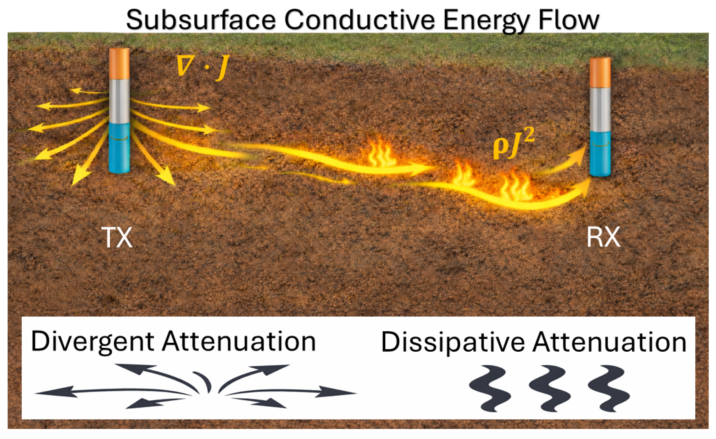
The signal intensity over an area is fundamentally dictated by two factors. The first factor is the material-dependent power dissipation derived from both contact resistance ($R_c$) and the losses due to current moving through the soil between the TX and RX ($\rho J^2$). The second factor is a reduction due to the divergence of the currents as they emanate away from the TX ($\nabla ·\mathbf{J}$). These two types of attenuation are illustrated in Figure 7. The reduction due to divergence is defined in (1). If the TTS system’s input impedance could be made mostly reactive, then the attenuation due to divergence could not be considered a loss since the source voltage would, ideally, be 90 degrees out of phase with the potential around the TX. This phase shift is experimentally shown in Figure 5a where the input voltage (top) leads the current (middle) waveform, showing that the inductive portion reduces the total power per pulse. The more reactive the TX would become, the greater the phase shift and the less active power would be injected. Here we will look at both the signal attenuation from divergence, and then the approximate attenuation due to resistive dissipation. It will be shown that the dissipative attenuation between locations actually reduces with increasing frequency (within the 20 kHz limit of the study).

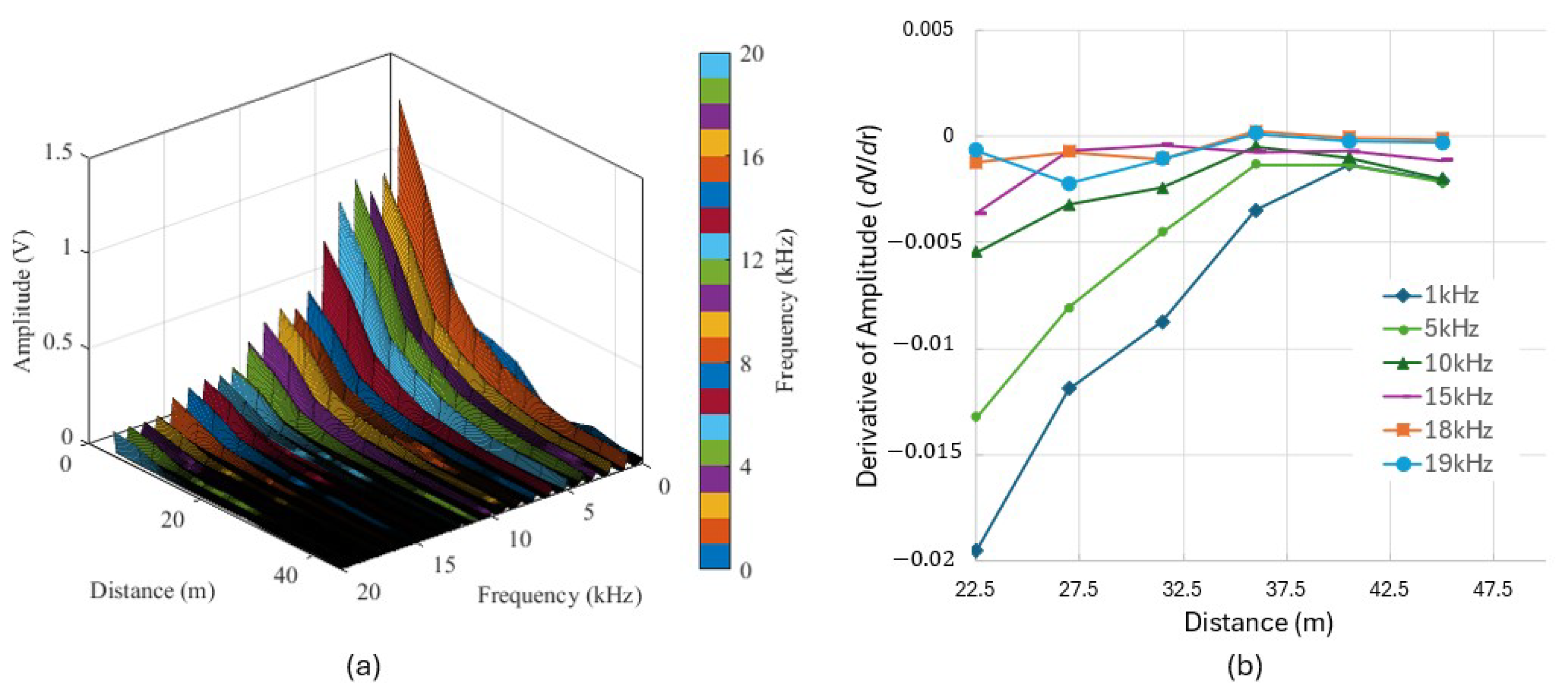
To study the signal attenuation over distance, we conducted a Fast Fourier Transform (FFT) at specific locations to characterize changes in the transmitted power signal. The setup included the transmitter station adjacent to an agricultural testing field. The transmitter station contained the pulse generator and the AFE connected to a battery bank as the power supply to inject current into the soil. An oscilloscope was used to record the resulting voltages in the ground vs time at the different measurement points along a path moving away from the TX. The FFT at each location was used to analyze the frequency components of the signal. Divergent attenuation is seen as an overall amplitude reduction in the FFT measurements from one location to another. The dissipative resistive losses are found by looking at the derivative of the changes in amplitude per frequency in the FFT, which are smaller changes between individual peaks over the same distance. These resistive losses in the soil are not expected to uniformly affect all frequencies.

4.1. Characterization of Distance-Dependent Divergent Attenuation

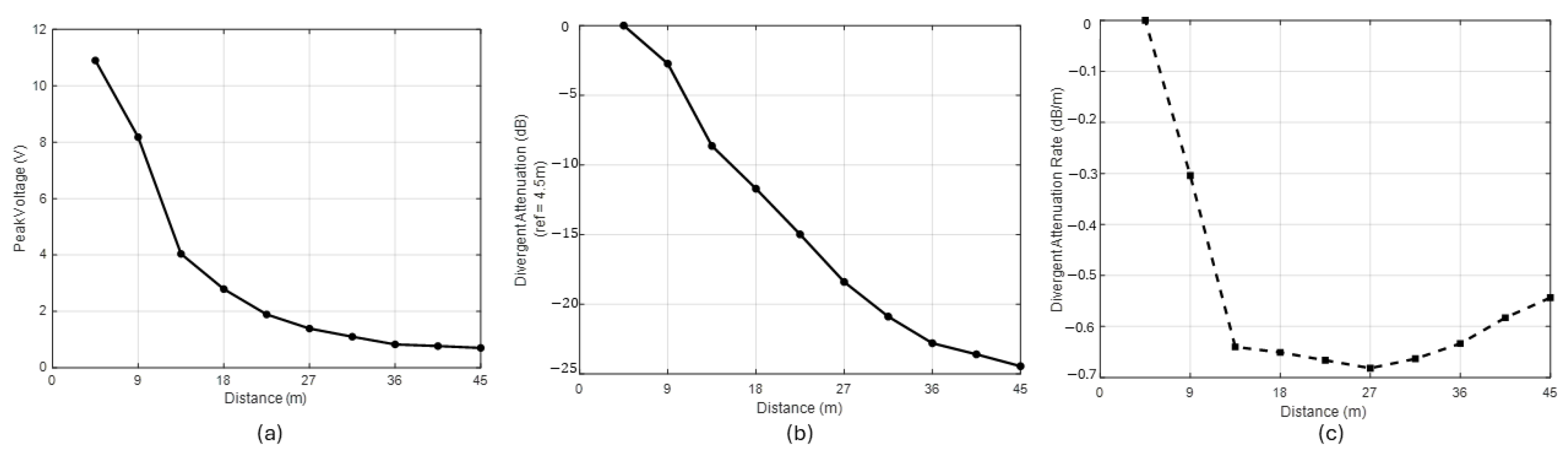
Figure 8a shows the peak voltage recorded in the time domain at each measurement location away from the TX. The measured amplitudes exhibit a distinct $1/r^2$-like decay, with peak voltage decreasing from approximately 11 V at 4.5 m to below 1 V at 45 m (note that this decay actually follows (4), which is $1/r-1/r^2$). The most pronounced attenuation occurs within the initial 13.5 m, which is to be expected from such a $1/r^2$ response. The Divergent Attenuation (${\alpha }_D$) in decibels (dB), as a function of frequency and distance, was evaluated by:

$${\alpha }_D(f,d)=20{\log }_{10}\left({\displaystyle \frac{\left|X_{\mathrm{d}}\left(f\right)\right|}{\left|X_{ref}\left(f\right)\right|}}\right)\left[\mathrm{dB}\right],$$

(18)

where $\left|X_d\left(f\right)\right|$ is the spectral amplitude at distance d, and $\left|X_{\mathrm{ref}}\left(f\right)\right|$ is the reference amplitude at $d_{\mathrm{ref}}=4.5\mathrm{m}$. This is shown in Figure 8b. By plotting the overall signal intensities in the FFT, the attenuation due to divergence of the currents underground is readily seen. The divergent attenuation increases monotonically to approximately −25 dB at 45 m. Taking the derivative of Figure 8b, $\left(A^{\prime }\left(d\right)={\displaystyle \frac{\mathrm{d}A}{\mathrm{d}d}}\right)$, yields the divergent attenuation’s rate of change (Figure 8c) over distance, which can be seen to reduce (the slope becomes positive) beyond 27 m.

4.2. Dissipative Attenuation

It is possible to determine subtle attenuation effects, unrelated to divergence, by analyzing differences between Fourier peaks at a given measurement location, and comparing them to the FFTs at other locations. While subtle, these differences can be used to determine frequencies that have less losses over the area, vs frequencies that may exhibit more loss as the currents travel away from the TX.

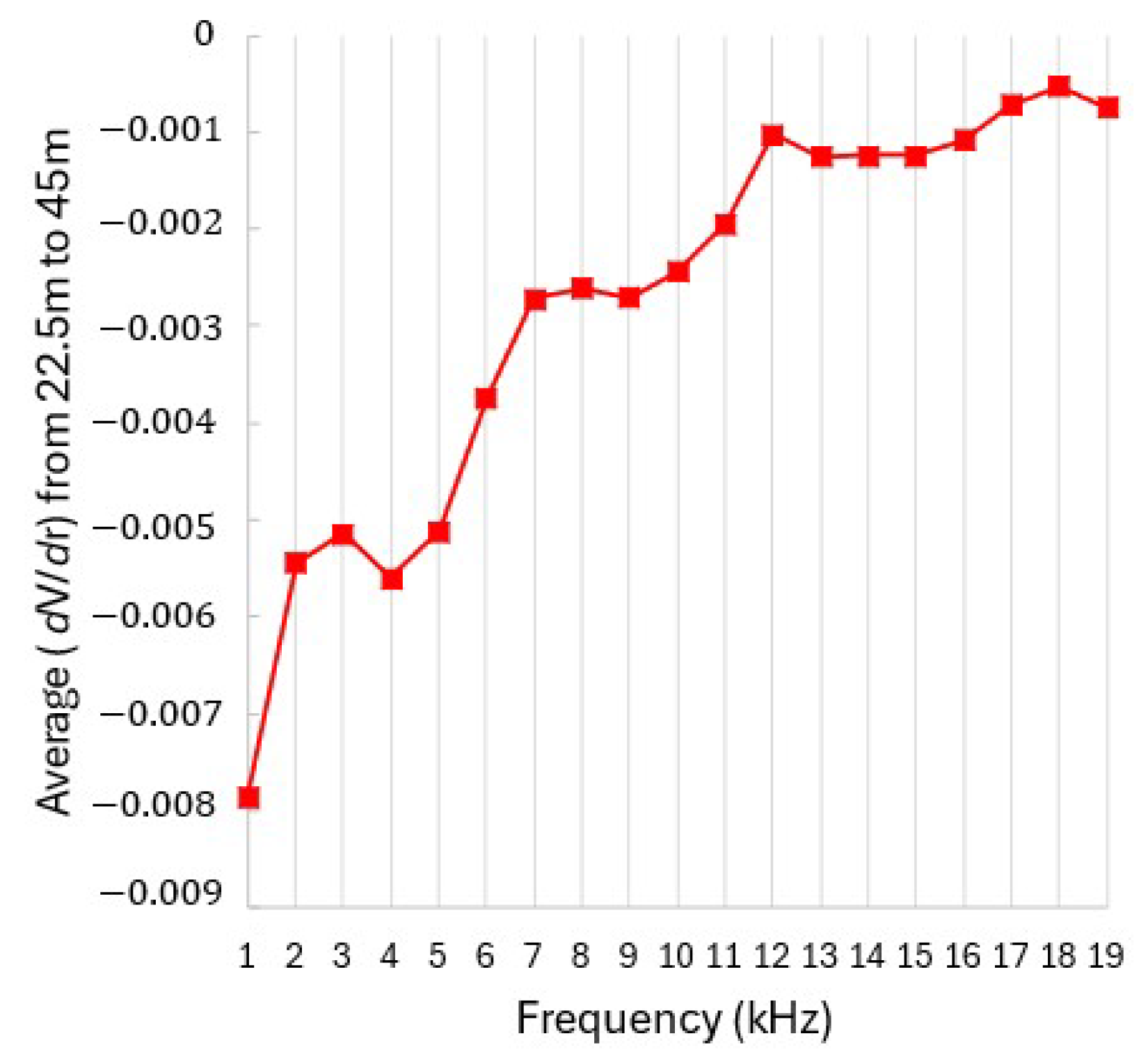
The FFTs at each measurement location, moving away from the TX, are shown in Figure 9a. To determine which frequency components had the least rate of change over the distance, which would correspond to the least resistive attenuation, we first restricted the response to distances of 22.5 m and beyond. this allows the effects of divergent attenuation to be minimized. We then took the derivative of the amplitude of each FFT component. Figure 9b is a plot of a truncated number of FFT components. As can be seen, as the frequency is increased, the rate of change encountered over the distance reduces. To further highlight the frequency trend over distance around the TTS system, the derivatives of Figure 9b for each frequency were averaged from a distance of 22.5 m to 45 m—this is shown in Figure 10. For frequencies 10 kHz and above, the rate of change is the lowest, and this trend appears to increase to a peak at 18 kHz and then begins to reduce.

4.3. Guidelines for Frequency Selection in a TTS System

The optimal operating frequency selection for the TTS system is determined through empirical frequency-domain attenuation analysis using the following procedure:

• Design the TTS transmitter to support low frequency operation. The transmitter should be capable of generating excitation signals within a frequency range where conduction currents are dominant and displacement currents are neglectible.
• Perform spatial frequency–response measurements. Field measurements of received signals should be taken at multiple locations along the a path away from the transmitter (TX). The Fourier transform of the received waveform at each location provides the amplitude of individual frequency components for comparison over distance.
• Focus on locations where the divergent effects of current are minimal. Divergence is encountered very close to the TX (within the first 10 m); these distances can be avoided when determining the optimum operation frequency. Readings in item II should be taken ideally at a 30 m or greater distance.
• Determine attenuation rates using spatial derivatives. For each frequency component, compute the derivative of FFT amplitude with respect to distance. This derivative quantifies how rapidly the field strength decays:
  • Lower magnitude derivative → lower attenuation.
  • Higher magnitude derivative → greater loss.
• Average attenuation metrics over the power transfer distance. To reduce local variability, derivative values should be averaged over the selected distance interval (e.g., 22.5–45 m). This produces a representative attenuation indicator for each frequency (such as shown in Figure 10).
• Identify frequencies with minimum amplitude decay. Frequencies exhibiting the smallest averaged derivative values correspond to reduced resistive (ohmic) losses and more efficient subsurface power transfer.
• Select the optimal operating band. Analysis shows attenuation decreases as frequency increases beyond the divergence-dominated regime due to the earth exhibiting more inductive reactance. Frequencies above approximately $10\mathrm{kHz}$ show lower attenuation, with a minimum observed near $18\mathrm{kHz}$. The preferred operating range for the location tested in this work was in the vicinity of 10–$18\mathrm{kHz}$.

Optimal TTS operating frequencies are those that minimize spatial amplitude decay after divergence effects are excluded, as determined from derivative analysis of FFT component amplitudes over distance.

5. Discussion

The results of Figure 9 and Figure 10 show that for higher operating frequencies, the energy loss in the soil reduces. This is consistent with Equation (4) which results in an inductive reactance within the soil. However, the reduction does not continue indefinitely with increasing frequency. From Figure 10, there is a peak at 18 kHz and then beyond the average rate of attenuation it starts to again increase (becoming more negative). It is expected that for higher frequencies, the slope of attenuation will continue to become more negative. We restricted our analysis to 20 kHz in this work as a continuation of the work presented in [10]. Future work will investigate frequencies beyond 20 kHz, with a greater emphasis on communications, since it was already shown that beyond 20 kHz power transfer is reduced.

From the data collected here, the observed attenuation is predominantly due to geometric spreading of the signal (what we defined as divergent attenuation), with minimal energy loss from dissipation. The reactive nature of the currents in the soil lead to a very different mechanism of energy dynamics, in direct contrast to radio antenna systems. In conventional radio, active power is made to leave the antenna and the geometric spreading of this active power flow creates the classic “$1/r^2$” loss found in every textbook. In TTS, it may be possible to design/adjust the soil conditions around the transmitter to maximize the reactive nature of the system. In this way signals will still reduce due to spread, but the power is not active but reactive, resulting in no loss due to geometric spreading of the current. As an analogy, a radio antenna is like a hose connected to a water reservoir which sprays water in all directions. Any water not captured by a receiver is lost, and the closer the receiver is the more water it can capture. The reactive power flow in a TTS system is more similar to a water fountain, where the hose sprays again in all directions but this water only falls into the pool of the fountain and is recycled. Thus, any water not captured by a receiver is simply recycled. The closer the receiver is, the more water it can collect, which ultimately takes from the main reservoir. If we now replace “the water” of this analogy with “energy” it is clear that the TTS system can function in a very different and more energy efficient manner, once optimized to maximize the reactive impedance of the transmitter.

6. Conclusions

In conclusion, this paper explores the reactive nature of the TTS system through the analysis of signal attenuation within a 50 m radius around the TTS TX. First, the original derivation was simplified to show that the earth around the TTS system can act as an inductive reactance. Next, an Active Front-End converter in tandem with an integration capacitor was used to create and rectify pulses. A method of approximating the average power in the pulses from oscilloscope measurements was presented. These pulses, having many fourier components, were then used to study attenuation up to 20 kHz. The results show that as the frequency is increased, the slope in attenuation reduces, indicating that less attenuation occurs at higher frequencies where the reactance is higher due to transmitter inductance. Future work will continue to investigate attenuation at larger distances, as the system is scaled. How to make the TTS transmitter more inductive will be a primary focus.

References

1. Luo, W.; Jackson, A.; Sorensen, J.; Dahal, A.; Goel, R.; Roundy, S.; Zesiger, C.; Young, D.J. Wireless Power Transfer Through Soil Over a Range of Moisture Levels for In-Situ Soil Health Monitoring. In Proceedings of the 2021 IEEE Sensors, Sydney, Australia, 31 October–3 November 2021; pp. 1–4. [Google Scholar] [CrossRef]
2. Ding, S.; Sanchez, J.; Jackson, A.; Roundy, S.; Goel, R.; Zesiger, C.; Young, D.J. Wireless Power Transfer Through Soil for Energizing an Underground Soil Moisture Sensor. In Proceedings of the 2022 IEEE Sensors, Dallas, TX, USA, 30 October–2 November 2022; pp. 1–4. [Google Scholar] [CrossRef]
3. Ding, S.; Sanchez, J.; Roundy, S.; Goel, R.; Zesiger, C.; Young, D.J. Land Vehicle-Based Wireless Power Transfer Through Soil for Enabling Batteryless Underground Soil Moisture Sensing Application. In Proceedings of the 2022 21st International Conference on Micro and Nanotechnology for Power Generation and Energy Conversion Applications (PowerMEMS), Salt Lake City, UT, USA, 12–15 December 2022; pp. 134–137. [Google Scholar] [CrossRef]
4. Niu, S.; Liu, W.; Liu, C.; Lyu, J.; Yang, C.; Chau, K.T. Wireless Power Transfer for IoT Bolts in Railways: Overcoming Coupling Challenges due to Conductive and Ferromagnetic Rails. IEEE Trans. Ind. Electron. 2025. [Google Scholar] [CrossRef]
5. Park, J.H.; Tran, N.M.; Hwang, S.I.; Kim, D.I.; Choi, K.W. Design and Implementation of 5.8 GHz RF Wireless Power Transfer System. IEEE Access 2021, 9, 168520–168534. [Google Scholar] [CrossRef]
6. Alcaraz López, O.L.; Suto, K. RF Energy Harvesting and Wireless Power Transfer for IoT. Sensors 2024, 24, 7567. [Google Scholar] [CrossRef] [PubMed]
7. Nusrat, T.; Roy, S.; Lotfi-Neyestanak, A.A.; Noghanian, S. Far-Field Wireless Power Transfer for the Internet of Things. Electronics 2022, 12, 207. [Google Scholar] [CrossRef]
8. Kim, S.; Vyas, R.; Bito, J.; Niotaki, K.; Collado, A.; Georgiadis, A.; Tentzeris, M.M. Ambient RF Energy-Harvesting Technologies for Self-Sustainable Standalone Wireless Sensor Platforms. Proc. IEEE 2014, 102, 1649–1666. [Google Scholar] [CrossRef]
9. Popović, Z.; Falkenstein, E.A.; Costinett, D.; Zane, R. Low-Power Far-Field Wireless Powering for Wireless Sensors. Proc. IEEE 2013, 101, 1397–1409. [Google Scholar] [CrossRef]
10. Nieman, B.; Johnson, C.S.; Pearce, M.; Marcrum, T.; Thorne, M.C.; Ashby, C.; Van Neste, C.W. Through the Soil Long Range Wireless Power Transfer for Agricultural IoT Networks. IEEE Trans. Ind. Electron. 2024, 71, 2090–2099. [Google Scholar] [CrossRef]
11. Bakkabulindi, G.; Hesamzadeh, M.R.; Amelin, M.; Da Silva, I.P. Planning algorithm for Single Wire Earth Return distribution networks. In Proceedings of the 2012 IEEE Power and Energy Society General Meeting, San Diego, CA, USA, 22–26 July 2012; pp. 1–7. [Google Scholar] [CrossRef]
12. Hosseinzadeh, N.; Mayer, J.E.; Wolfs, P.J. Rural Single Wire Earth Return distribution networks—Associated problems and cost-effective solutions. Int. J. Electr. Power Energy Syst. 2011, 33, 159–170. [Google Scholar] [CrossRef]
13. Kashem, M.A.; Ledwich, G. Impact of distributed generation on protection of single wire earth return lines. Electr. Power Syst. Res. 2002, 62, 67–80. [Google Scholar] [CrossRef]
14. Johnson, C.S.; Tidwell, M.; Marcrum, T.; Stump, W.; Van Neste, C.W. Improving the Effective Range of a Through the Soil Long Range Wireless Power Transfer System Using a Marx Inverter Topology. In Proceedings of the 2024 IEEE Wireless Power Technology Conference and Expo (WPTCE), Kyoto, Japan, 8–11 May 2024; pp. 257–260. [Google Scholar] [CrossRef]
15. Ufer, H.G. Investigation and Testing of Footing-Type Grounding Electrodes for Electrical Installations. IEEE Trans. Power Appar. Syst. 1964, 83, 1042–1048. [Google Scholar] [CrossRef]
16. Daily, W. A new method for characterization of downhole antennas used in geophysical probing. Geophys. Res. Lett. 1982, 9, 507–509. [Google Scholar] [CrossRef]
17. National Bureau of Standards. National Electrical Safety Code: Grounding Rules and Parts I, II, III, IV, and V; Technical Report NBS HB 30; National Bureau of Standards: Gaithersburg, MD, USA, 1948. [Google Scholar] [CrossRef]
18. Dwight, H.B. Calculation of Resistances to Ground. Trans. Am. Inst. Electr. Eng. 1936, 55, 1319–1328. [Google Scholar] [CrossRef]
19. Jacob, P.; Lippert, G.; Matsch, L.; Philip, B.; Smith, G. Bibliography on Ground Resistance and Potential Gradient Measurements AIEE Committee Report. Trans. Am. Inst. Electr. Engineers. Part III Power Appar. Syst. 1960, 79, 52–58. [Google Scholar] [CrossRef]
20. Cagniard, L. Basic theory of the magneto-telluric method of geophysical prospecting. Geophysics 1953, 18, 605–635. [Google Scholar] [CrossRef]
21. Shi, J.; Wang, F.; Zhang, D.; Huang, H.; Wu, Y. Refined numerical simulation of signal propagation in soils for wireless underground sensor networks. Tunn. Undergr. Space Technol. 2023, 140, 105312. [Google Scholar] [CrossRef]
22. Lauro, S.E.; Mattei, E.; Cosciotti, B.; Di Paolo, F.; Arcone, S.A.; Viccaro, M.; Pettinelli, E. Electromagnetic signal penetration in a planetary soil simulant: Estimated attenuation rates using GPR and TDR in volcanic deposits on Mount Etna. J. Geophys. Res. Planets 2017, 122, 1392–1404. [Google Scholar] [CrossRef]
23. Rüdenberg, R. Grounding principles and practice I—Fundamental considerations on ground currents. Electr. Eng. 1945, 64, 1–13. [Google Scholar] [CrossRef]
24. Tidwell, M.; Swindell, C.; Johnson, C.S.; Gupta, M.; Van Neste, C.W. Wireless Communication of Buried IoT Sensors Utilizing Through the Soil Wireless Power Transfer for Precision Agriculture. In Proceedings of the 2023 IEEE Wireless Power Technology Conference and Expo (WPTCE), San Diego, CA, USA, 4–8 June 2023; pp. 1–5. [Google Scholar] [CrossRef]
Figure 1. Illustration of the TTS system showing wireless power transmission from solar panel arrays to receivers in an agricultural field through subsurface conduction currents. (a) Power-flow diagram of the energy conversion and injection stages. (b) Overall system architecture; the subsystem investigated in this paper is highlighted by the dotted square.
Energies 19 01080 g001
Figure 2. Circuit model of the TTS system where R C is the contact resistance of the TX or RX electrodes, and L T X / R X is the total inductance formed from currents flowing through the subsurface. (a) Illustration of the system’s geometric configuration. (b) Circuit model derived in [10]. Note that the AFE topology is discussed in the following section. It is used to generate the depicted current pulse train whose Fourier analysis gives insight into the signal attenuation over distance.
Energies 19 01080 g002
Figure 3. Proposed prototype of the inverter–AFE interface with differentiating capacitor C DIF . (a) Schematic diagram. (b) Experimental setup.
Energies 19 01080 g003
Figure 4. Timing diagram of the capacitor-coupled inverter–AFE interface. Q and Q ¯ represent the inverter switching signals, while S and S ¯ represent the switching signals of the Active Front End converter.
Energies 19 01080 g004
Figure 5. Field Measurements. (a) Input voltage and current transients with corresponding Instantaneous power (b) Open-field measurement arrangement showing voltage sensing rods, receiver well, and the transmitter location (off-image), with a line showing the direction of current emanating from the TX.
Energies 19 01080 g005
Figure 7. Illustration of the two types of attenuation in a TTS system. The divergent attenuation is due to the spreading out of the power signal with distance. Since the current would be ideally 90 degrees out of phase with the source voltage, divergent spread is not a loss in power. In contrast, the dissipative attenuation is directly related to conducted power losses in the subsurface.
Energies 19 01080 g007
Figure 8. Time domain attenuation behavior. (a) Peak voltage versus distance. (b) Attenuation relative to the 4.5 m reference. (c) Attenuation rate, defined as the numerical derivative of the attenuation curve, A ( d ) = d A d d .
Energies 19 01080 g008
Figure 9. FFT data taken at measurement points moving away from the TX. (a) 3D plot of the FFT spectra for all measurement locations. (b) The derivative of the FFT data for a truncated frequency set focusing on distances where divergent attenuation has greatly reduced. Note that higher frequency components have less changes over the distance.
Energies 19 01080 g009
Figure 10. A plot where the value of the derivative of the FFT, from 22.5 m to 45 m, was averaged to a single value for each frequency. This shows the average amplitude change per frequency over a distance where divergent attenuation is neglectable, showing only average changes due to dissipative (resistive) attenuation.
Energies 19 01080 g010
Disclaimer/Publisher’s Note: The statements, opinions and data contained in all publications are solely those of the individual author(s) and contributor(s) and not of MDPI and/or the editor(s). MDPI and/or the editor(s) disclaim responsibility for any injury to people or property resulting from any ideas, methods, instructions or products referred to in the content.