Computationally Efficient Online Adaptation Method for PM Machine LPTN Model

Abstract

Accurate long-term temperature prediction is critical for the reliable operation of mass-produced electrical machines. However, due to the randomness inherent in the manufacturing process, machines with identical design parameters often exhibit distinct thermal properties. The aging of the insulation system can also lead to variation in thermal performance. Conventional lumped-parameter thermal network (LPTN) models with fixed parameters fail to account for these factors, thus leading to biased prediction results for long-term temperature forecasting of mass-produced machines. To enhance the robustness of LPTN models, this paper proposes a methodology for adaptive online parameter updating. Based on the mathematical formulation of LPTN, a fast Jacobian matrix calculation method for model prediction errors is developed, which avoids the time-consuming numerical computation process. To further alleviate the computational burden, key parameters with significant impacts on prediction errors are screened prior to each optimization iteration. These improvements collectively reduce computational resource requirements and enable real-time online implementation. Finally, experimental verification is conducted on a 10 kW permanent magnet machine. Comparative analyses against the numerical method and extended Kalman filter (EKF) demonstrate that the proposed method can be efficiently realized and is more effective in estimating the model parameters online.

1. Introduction

Permanent magnet (PM) synchronous machines are widely used in various applications due to their high-performance character. To protect the vulnerable machine winding, avoid overheating, and enable thermal management, temperature information is usually indispensable [1] and can be acquired through thermal sensors or thermal models [2]. The thermal sensor can provide the most reliable real-time temperature information. However, the long-term variation cannot be effectively predicted. On the other hand, thermal models are widely used for electrical machine thermal performance prediction [3,4,5,6,7], whereas the development of a proper thermal model for PM machines is not an easy task [8,9].

Currently, three thermal-modeling methods are widely used, i.e., the finite element method (FEM), computational fluid dynamics (CFD), and lumped-parameter thermal network (LPTN) [10]. The CFD method and FEM enjoy high precision, whereas the computation costs make them inappropriate for online applications. The LPTN models can provide decent results with much less calculation effort, which makes them widely used in online thermal prediction for electrical machines [11,12] and power electronic devices [13,14]. Due to the complicated structure and the involvement of various materials, the criteria of the PM machine LPTN model are not well defined and are highly dependent on the experience of developers [15]. Furthermore, some equivalent model parameters representing the heat transfer effect of a complicated process cannot be easily analytically determined [6]. To solve this problem, the experimental data are usually combined with machine prior knowledge to calibrate LPTN model parameters [16]. In practice, the resources and time are limited, and the experimental data cannot cover a machine’s full working conditions. The aging of the machine also influences its thermal properties [17]. At the same time, due to the uncertainty of the manufacturing process and randomness of the winding arrangement, machines with the same design parameters may possess varied thermal performance. All these restrict the application scope of an LPTN model developed in the lab. Thus, conventional LPTN models may not be robust enough for mass-produced PM machine long-term thermal prediction.

Some researchers have been trying to solve this problem. In [18], the Kalman Filter (KF) was used to adaptively tune the thermal elastic error model for a three-axis CNC machine. A kind of LPTN model and flux observer were fused in [19] and combined with KF to improve the estimated PM temperature of a PM machine. The widely used KF method can improve the LPTN model output by manipulating the model states, while the model parameters are kept unchanged. In other words, although the instant model output has been improved, the model itself is not modified. As the parameters of the LPTN model are nonlinear with model output, some researchers used the Extended Kalman Filter (EKF) to adaptively estimate model parameters online [20,21]. In this process, the model parameters are merged into the state, so the parameters and states can be tuned together. However, directly modifying model states may deteriorate the precision of the estimated parameters. In addition, the model parameters may have different magnitude ranges, which could lead the local numerical model used in the EKF to diverge.

In this paper, a method to adaptively update the LPTN model parameters online is proposed. Based on the mathematical description of the LPTN model, a fast calculation method for the model prediction error Jacobian matrix is proposed. And this makes it so that the gradient-based optimization calculation can be efficiently realized online. Thus, the robustness of the LPTN model can be adaptively improved.

Notably, standard mass-produced PM motors are rarely equipped with full sets of embedded temperature sensors, unlike the prototype in this study, due to cost constraints. In practice, after the LPTN model is developed and validated in the laboratory, the proposed method can be directly applied to online operation and parameter optimization. The proposed method does not impose any restrictions on the number of measured feedback temperatures during online optimization, meaning that full temperature feedback is not a prerequisite for its implementation. Instead, online optimization can be achieved using limited temperature sensors that are easy to install, such as those mounted on the stator winding ends and motor housing. On the other hand, some sensorless methods (stator winding resistance detection) can also be adopted to indirectly obtain the winding temperature when physical sensors are unavailable. This helps improve the adaptability to standard production motors without additional hardware costs

The structure of this paper is as follows. In Section 2, the LPTN model is established, and the mathematical description is derived. The offline parameter identification process is given in Section 3. After that, Section 4 explains the basic algorithm of the proposed model parameter adaptation method. The experimental verification and comparison with the numerical and EKF methods are demonstrated in Section 5. Finally, Section 6 concludes the paper.

2. The Establishment of the LPTN Model

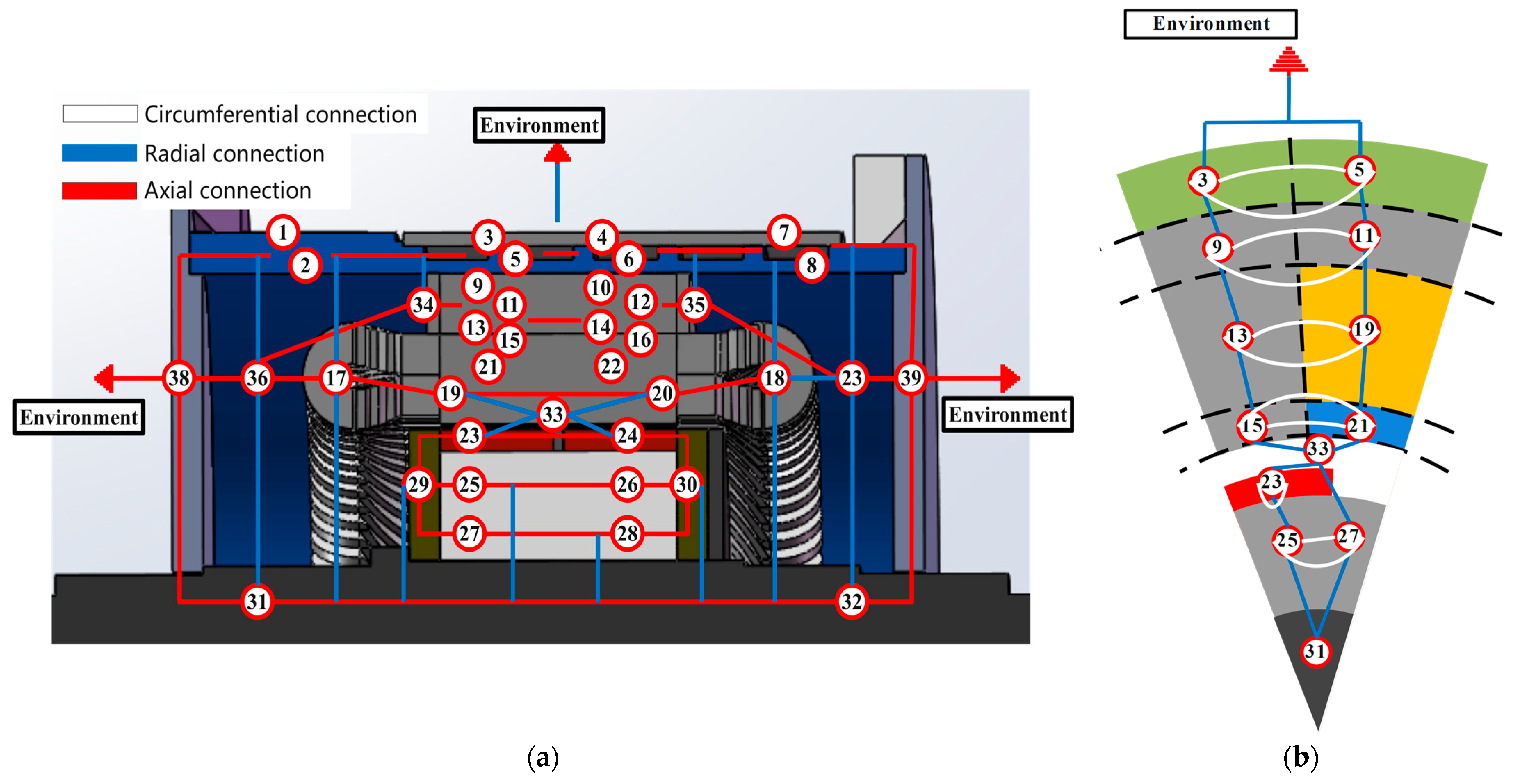
A three-dimensional LPTN model is established and shown in Figure 1. The definition of each node is given in

Table 1. The node definition in the LPTN model.

Node	Machine Part	Node	Machine Part
1–8	Housing	25–28	Rotor iron
9–12	Yoke	29–30	Rotor core retaining plate
13–16	Tooth	31–32	Shaft
17–18	End winding	33	Air gap
19–20	Slot winding	34–35	Stator core retaining plate
21–22	Slot wedge	36–37	End space
23–24	PM	38–39	End cap

.

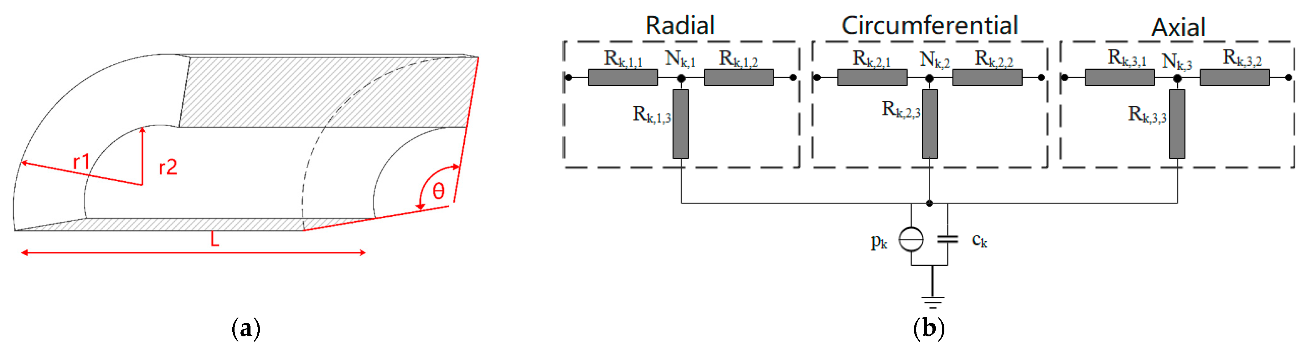
In this LPTN model, each node comprises several thermal resistances and one thermal capacitance. Nodes 1–28 are established through the T-modeling method [20]. The corresponding machine components of these nodes are meshed into basic arc elements [21], as shown in Figure 2. Thermal resistances in these nodes can be calculated based on machine structural and material properties, as summarized in

Table 2. The thermal resistance definition in the T model.

Index	Radial	Axial	Circumference
1	${\displaystyle \frac{1}{2\theta L{k}_r}}\left[{\displaystyle \frac{2\ln \left(\frac{{\mathrm{r}}_2}{{\mathrm{r}}_1}\right)r_2^2}{r_2^2-r_1^2}}-1\right]$	${\displaystyle \frac{L}{k_a\theta \left(r_2^2-r_1^2\right)}}$	${\displaystyle \frac{\theta }{2L{k}_c\ln \left(\frac{{\mathrm{r}}_2}{{\mathrm{r}}_1}\right)}}$
2	${\displaystyle \frac{1}{2\theta L{k}_r}}\left[1-{\displaystyle \frac{2\ln \left(\frac{{\mathrm{r}}_2}{{\mathrm{r}}_1}\right)r_1^2}{r_2^2-r_1^2}}\right]$	${\displaystyle \frac{L}{k_a\theta \left(r_2^2-r_1^2\right)}}$	${\displaystyle \frac{\theta }{2L\ln \left(\frac{{\mathrm{r}}_2}{{\mathrm{r}}_1}\right)k_c}}$
3	${\displaystyle \frac{-1}{4\theta L{k}_r}}\left[{\displaystyle \frac{r_2^2+r_1^2}{r_2^2-r_1^2}}-{\displaystyle \frac{4\ln \left(\frac{{\mathrm{r}}_2}{{\mathrm{r}}_1}\right)r_1^2{r}_2^2}{{\left(r_2^2-r_1^2\right)}^2}}\right]$	${\displaystyle \frac{L}{k_{a}3\theta \left(r_2^2-r_1^2\right)}}$	${\displaystyle \frac{\theta }{{12Lk}_c}}\left[{\displaystyle \frac{r_2^2+r_1^2}{r_2^2-r_1^2}}-3\ln \left({\displaystyle \frac{r1}{r_2}}\right)\right]$

[20,21]. $k_r$, $k_a$, and $k_c$ are the thermal conductances in the radial, axial, and circumferential directions. $P_k$ and $c_k$ are the loss and thermal capacitance of the kth node. $R_{k,i,j}$ denotes the $j$th thermal resistance in the i direction (1, 2, and 3 denote radial, circumferential, and axial) of the kth node. The thermal capacitance of the $k$th node can be calculated through

$$c_k=c_{\rho }\rho {\displaystyle \frac{\theta }{2}}L\left(r_2^2-r_1^2\right)$$

(1)

where $c_{\rho }$, $\rho$ are the specific thermal capacitance and density.

Nodes 29–38 represent complicated structures. Thus, they are modeled through equivalent thermal resistance and capacitance. Detailed modeling ideas and techniques can be found in [22,23,24]. The mathematical description of the established LPTN model can be explicitly derived as

$$\mathit{C}{\displaystyle \frac{d\mathit{T}}{dt}}=\mathit{P}-{\mathit{R}}_1\mathit{T}+{\mathit{R}}_2\mathit{N}+{\mathit{R}}_{u1}{\mathit{U}}_{\mathit{C}}$$

(2)

$${\mathit{R}}_3\left(\mathit{K}\mathit{T}-\mathit{N}\right)={\mathit{R}}_4\mathit{N}+{\mathit{R}}_5\mathit{K}\mathit{T}-{\mathit{R}}_{u2}{\mathit{U}}_{\mathit{C}}$$

(3)

where

$$\mathit{T}={\left[T_1,T_2,\dots T_{39}\right]}^T$$

(4)

$$\mathit{P}={\left[p_1,p_2,\dots p_{39}\right]}^T$$

(5)

$$\mathit{C}=diag\left(c_1,c_2,\dots c_{39}\right)$$

(6)

$$\mathit{N}={\left[N_{\mathrm{1,1}},N_{\mathrm{1,2}},\dots N_{\mathrm{28,3}},0,\dots 0\right]}^T$$

(7)

$${\mathit{R}}_1=\left[\begin{array}{cc}{R}_{T1}& 0\\ 0& R_{c1}\end{array}\right]$$

(8)

$${\mathit{R}}_2=\left[\begin{array}{cc}{R}_{T2}& 0\\ R_{c2}& 0\end{array}\right]$$

(9)

$${\mathit{R}}_3=diag\left({\displaystyle \frac{1}{R_{\mathrm{1,1},3}}},{\displaystyle \frac{1}{R_{\mathrm{1,2},3}}},\dots {\displaystyle \frac{1}{R_{\mathrm{28,3},3}}},\mathrm{1,1},\dots 1\right)$$

(10)

$${\mathit{R}}_4=\left[\begin{array}{cc}{R}_{T4}& 0\\ 0& 0\end{array}\right]$$

(11)

$${\mathit{R}}_5=\left[\begin{array}{cc}0& R_{T5}\\ 0& E\end{array}\right]$$

(12)

$${\mathit{R}}_{T1}=diag\left(\sum _{i=1}^3{\displaystyle \frac{1}{R_{1,i,3}}},\sum _{i=1}^3{\displaystyle \frac{1}{R_{2,i,3}}},\dots \sum _{i=1}^3{\displaystyle \frac{1}{R_{28,i,3}}}\right)$$

(13)

$${\mathit{R}}_{c1}=\left[\begin{array}{ccc}{\displaystyle \sum _{i=\begin{array}{c}1N1,\dots 28N3,\\ 29,\dots 39,e\end{array}}}{\displaystyle \frac{1}{R_{i,29}}}& \dots & -{\displaystyle \frac{1}{R_{\mathrm{39,29}}}}\\ ⋮& \ddots & ⋮\\ -{\displaystyle \frac{1}{R_{\mathrm{29,39}}}}& \dots & {\displaystyle \sum _{i=\begin{array}{c}1N1,\dots 28N3,\\ 29,\dots 39,e\end{array}}}{\displaystyle \frac{1}{R_{i,39}}}\end{array}\right]$$

(14)

$${\mathit{R}}_{T2}=\left[\begin{array}{ccc}\begin{array}{ccc}{\displaystyle \frac{1}{R_{\mathrm{1,1},3}}}& {\displaystyle \frac{1}{R_{\mathrm{1,2},3}}}& {\displaystyle \frac{1}{R_{\mathrm{1,3},3}}}\end{array}& & \\ & \ddots & \\ & & \begin{array}{ccc}{\displaystyle \frac{1}{R_{\mathrm{28,1},3}}}& {\displaystyle \frac{1}{R_{\mathrm{28,2},3}}}& {\displaystyle \frac{1}{R_{\mathrm{28,3},3}}}\end{array}\end{array}\right]$$

(15)

$${\mathit{R}}_{c2}=\left[\begin{array}{ccc}{\displaystyle \frac{1}{R_{1N\mathrm{1,29}}}}& \dots & {\displaystyle \frac{1}{R_{28N\mathrm{3,29}}}}\\ ⋮& \ddots & ⋮\\ {\displaystyle \frac{1}{R_{1N\mathrm{1,39}}}}& \dots & {\displaystyle \frac{1}{R_{28N\mathrm{3,39}}}}\end{array}\right]$$

(16)

$${\mathit{R}}_{u1}={\left[0,\dots ,0,{\displaystyle \frac{1}{R_{e,28}}},\dots ,{\displaystyle \frac{1}{R_{e,39}}}\right]}^T$$

(17)

$${\mathit{R}}_{T4}=\left[\begin{array}{ccc}{\displaystyle \sum _{i=\begin{array}{c}1N1,\dots 28N3,\\ 29,\dots 39,e\end{array}}}{\displaystyle \frac{1}{R_{i,1N1}}}& \dots & -{\displaystyle \frac{1}{R_{28N\mathrm{3,1}N1}}}\\ ⋮& \ddots & ⋮\\ -{\displaystyle \frac{1}{R_{1N1,28N3}}}& \dots & {\displaystyle \sum _{i=\begin{array}{c}1N1,\dots 28N3,\\ 29,\dots 39,e\end{array}}}{\displaystyle \frac{1}{R_{i,28N3}}}\end{array}\right]$$

(18)

$${\mathit{R}}_{T5}=\left[\begin{array}{ccc}-{\displaystyle \frac{1}{R_{\mathrm{29,1}N1}}}& \dots & -{\displaystyle \frac{1}{R_{\mathrm{39,1}N1}}}\\ ⋮& \ddots & ⋮\\ -{\displaystyle \frac{1}{R_{\mathrm{29,28}N3}}}& \dots & -{\displaystyle \frac{1}{R_{\mathrm{39,28}N3}}}\end{array}\right]$$

(19)

$${\mathit{R}}_{u2}={\left[{\displaystyle \frac{1}{R_{e,1N1}}},\dots ,{\displaystyle \frac{1}{R_{e,28N3}}},0,\dots ,0\right]}^T$$

(20)

$$\mathit{K}=\left[\begin{array}{cc}\begin{array}{ccc}1& & \\ 1& & \\ 1& & \\ & \ddots & \\ & & 1\\ & & 1\\ & & 1\end{array}& \\ & {\mathit{E}}_{\mathbf{11}}\end{array}\right]$$

(21)

where $T_k$ represents the temperature of the $k$th node; $N_{i,j}$ denotes the temperature of the $N_{i,j}$point in the $i$th T node, as illustrated in Figure 2b; $U_C$is the ambient temperature vector; and $R_{i,k}$ is the resistance between the i and k node. $1/R_{i,i}$ equals zero. Subscript $iNj$ denotes the $N_{i,j}$point and $e$ represents the ambient. With (2) and (3), the mathematical description of the established LPTN model can be derived

$${\displaystyle \frac{d\mathit{T}}{dt}}={\mathit{C}}^{-1}\mathit{P}+{\mathit{C}}^{-1}\mathit{A}\mathit{T}+{\mathit{C}}^{-1}\mathit{B}{\mathit{U}}_{\mathit{C}}$$

(22)

$$\mathit{A}={\mathit{R}}_2{\left({\mathit{R}}_3+{\mathit{R}}_4\right)}^{-1}\left({\mathit{R}}_3-{\mathit{R}}_5\right)\mathit{K}-{\mathit{R}}_1$$

(23)

$$\mathit{B}={\mathit{R}}_2{\left({\mathit{R}}_3+{\mathit{R}}_4\right)}^{-1}{\mathit{R}}_{u2}+{\mathit{R}}_{u1}$$

(24)

The corresponding discrete model can be obtained through the one-step Euler method.

$$\mathit{T}\left(n+1\right)={\mathit{M}}_T\mathit{T}\left(n\right)+{\mathit{M}}_P\mathit{P}+{\mathit{M}}_U{\mathit{U}}_{\mathit{C}}$$

(25)

where

$${\mathit{M}}_P=∆t{\mathit{C}}^{-1}$$

(26)

$${\mathit{M}}_T=∆t{\mathit{C}}^{-1}\mathit{A}+\mathit{E}$$

(27)

$${\mathit{M}}_U=∆t{\mathit{C}}^{-1}\mathit{B}$$

(28)

It should be noted that the one-step Euler method is selected for discretization primarily to balance computational efficiency and real-time performance. While the trapezoid method offers higher accuracy, it requires solving implicit equations, which increases the computational burden and is not suitable for this specific requirement.

The LPTN model established above can be used to predict the spatial temperature distribution of the electrical machine, provided all the parameters are appropriately defined. Based on the results presented in Table 2, it can be found that the model thermal resistances are related to both machine physical parameters and material thermal properties. Explicitly and analytically determining all the thermal parameters is very demanding, if not impossible. To obtain reasonable initial thermal parameters, offline parameter estimation is used and is demonstrated in the following section.

3. Offline Parameter Estimation Process

To estimate difficult to determine thermal parameters, experimental data-based offline parameter estimation is processed in this section.

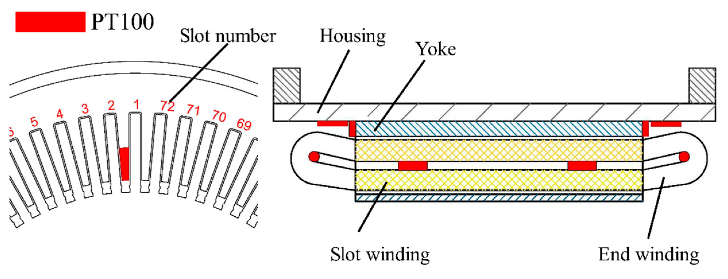
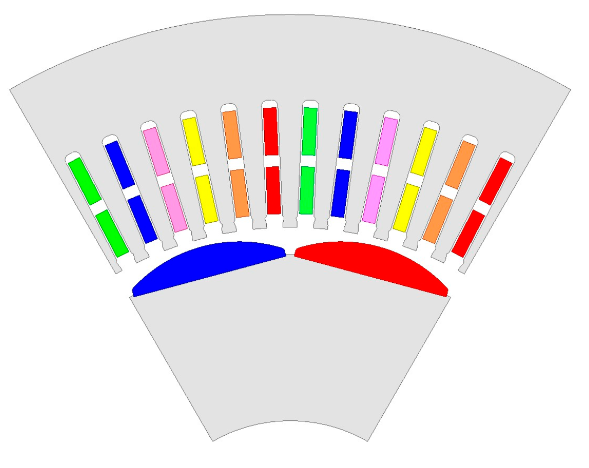
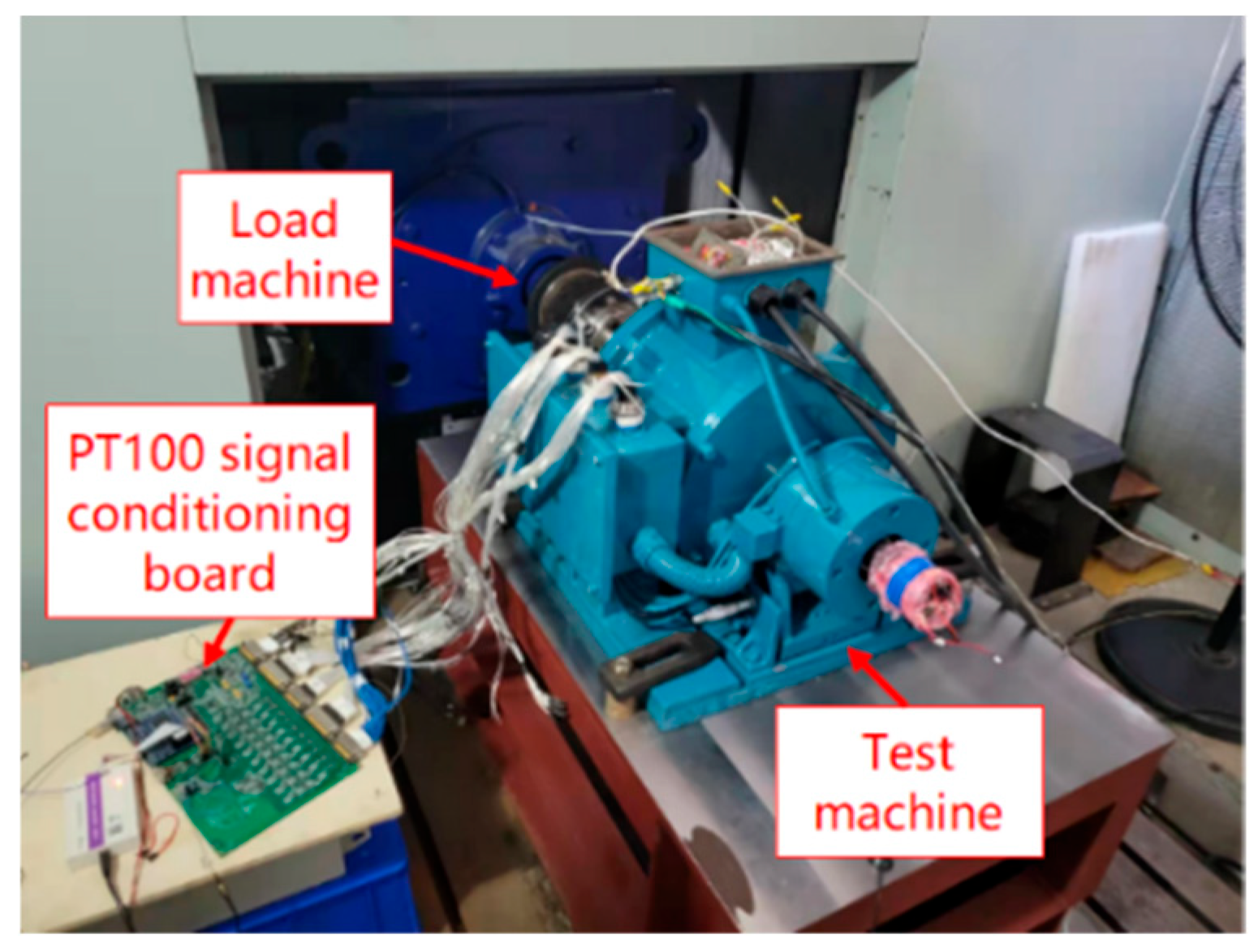
The test machine is a 10 kW PM machine with thermal sensors, PT100s, embedded in different parts. The distribution of these sensors is demonstrated in Figure 3. The main parameters are tabulated in

Table 3. Machine parameters.

Parameter	Value
Rated speed	900 rpm
Pole number	12
Rated power	10 kW
Outer diameters	290 mm
Stack Length	92 mm

. The topology of the machine and the experimental setup can be seen in Figure 4 and Figure 5, respectively. The load machine provides various loads, and the test machine is controlled through the inverter and double-closed loop method. The signal of these PT100 sensors is transferred to PC and processed in Labview. The temperature signal is sampled at about 1 Hz.

The parameter estimation is based on the mathematical description of the LPTN model derived in Section 2. The losses $\mathit{P}$ comprise copper loss, iron loss, PM loss, and mechanical loss. The copper loss is derived from measured stator current and temperature-dependent resistance. Iron and PM losses are simulated via the FEM. Mechanical loss is neglected in this process. And the total loss is verified using the efficiency data obtained from experiments. Once the initial temperature $\mathit{T}\left(0\right)$, environmental temperature ${\mathit{U}}_{\mathit{C}}$, and losses $\mathit{P}$ are determined, the LPTN model-predicted results under a set of thermal parameters could be acquired through (25). As not all node temperatures defined in the LPTN model are measured, the model output that corresponds to measured points can be expressed as

$$\mathit{Y}\left(t\right)={\mathit{S}}_{\mathit{m}}\mathit{T}\left(t\right)$$

(29)

where ${\mathit{S}}_{\mathit{m}}$ is the selection matrix. Thus, the target is to obtain a set of thermal parameters $\mathit{\Gamma }=\left[{\mathsf{\Gamma }}_{\mathbf{1}},{\mathsf{\Gamma }}_{\mathbf{2}},\dots {\mathsf{\Gamma }}_{\mathit{n}}\right]$ that minimize the sum squared error (SSE) of the prediction

$$\epsilon =SSE\left(\mathit{Y}\left(\mathit{\Gamma }\right)-{\mathit{Y}}_{\mathit{m}}\right)$$

(30)

where ${\mathit{Y}}_{\mathit{m}}$ is the measured temperature data, $\mathit{\Gamma }$ denotes the vector of thermal parameters to be optimized, and $\mathit{Y}\left(\mathit{\Gamma }\right)$ is the LPTN model-predicted results under the thermal parameters $\mathit{\Gamma }$:

$$\mathit{Y}\left(\mathit{\Gamma }\right)=\left[\begin{array}{c}\begin{array}{c}\mathit{Y}\left(1,\mathit{\Gamma }\right)\\ \mathit{Y}\left(2,\mathit{\Gamma }\right)\\ ⋮\\ \mathit{Y}\left(k,\mathit{\Gamma }\right)\end{array}\end{array}\right]$$

(31)

where $\mathit{Y}\left(k,\mathit{\Gamma }\right)$ is the model-predicted result at time $k$.

A kind of two-step optimization method was adopted here. First, the genetic algorithm (GA) was utilized to search for the optimal parameters in a wide variation range. When the GA stops, the sequential quadratic programming (SQP) method continues pursuing the optimal value and generates the final estimated parameter. The estimation process was realized in Matlab R2023a (The MathWorks, Inc., Natick, MA, USA) and based on various DC and AC experimental data. To consider the temperature effect, the copper loss under temperature $T_w$ was updated through

$$P_w\left(T_w\right)=P_{w20}\left(1+\alpha \left(T_w-20°\mathrm{C}\right)\right)$$

(32)

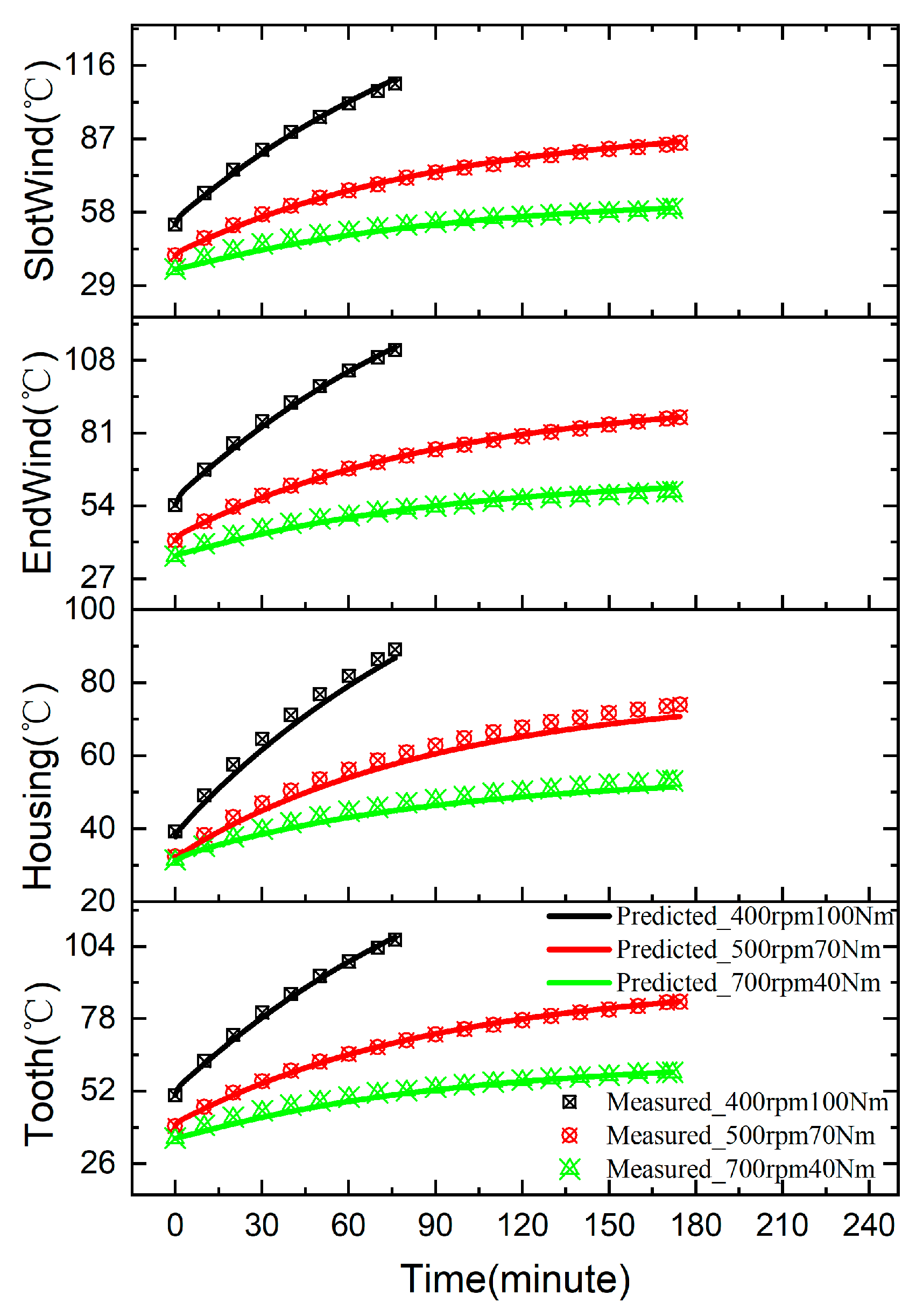
where $P_{w20}$ is the copper loss calculated under $20°\mathrm{C}$ and α is the copper temperature coefficient, adopted as $3.93\times {10}^{-3}/℃$. The core loss and PM loss were obtained through the FEM. Most LPTN model parameters were estimated based on DC experimental data. The speed-sensitive equivalent parameters, e.g., those connected with the shaft, airgap, and end region were estimated based on the data obtained under different speeds and interpolated with respect to speed. These parameters are closely tied to rotational conditions. Theoretically, the rotation of the motor rotor affects the heat transfer between the stator and rotor, as variations in rotational speed directly alter the convective heat exchange within the airgap. To validate both the effectiveness of these offline-estimated parameters and the applicability of the model across different working conditions, the model performance is demonstrated in Figure 6. The results indicate that the LPTN model incorporating these estimated parameters achieves satisfactory prediction accuracy under various working conditions. These parameters will subsequently serve as the initial values for the adaptation process presented hereafter.

4. Methodology of the Proposed LPTN Model Adapta-Tion Method

In this section, an algorithm to adaptively update the LPTN model parameters online will be introduced. The basic idea lies in reducing the calculation burden of the gradient-based optimization method and enabling the corresponding computation to be efficiently realized. Thus, based on the measured data, the LPTN model parameters can be tuned online. For parameter changes induced by aging in a single electrical machine, the key thermal parameters can be updated in real time based on measured temperature feedback, compensating for gradual performance degradation. For manufacturing-related parameter inconsistency, the parameters estimated offline are chosen as initial values and tuned online based on unique measured data, thus calibrating the model to match individual thermal characteristics. The basic algorithm will be introduced here, and the experimental verification will be demonstrated in the next section.

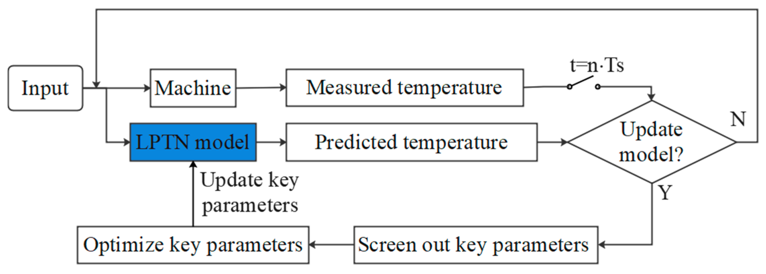
The whole process is illustrated in Figure 7. Every $T_s$ time, the measured temperatures will be compared with the LPTN model predicted results. If the prediction error becomes large, it is supposed that the LPTN model needs to be updated. Then, the prominent inappropriate LPTN model thermal parameters are screened out and updated through the optimization algorithm. As with the offline parameter estimation process, the target here is still to find the proper parameter value that minimizes the prediction error. However, a time-consuming stochastic optimization method, like GA, is not appropriate for online realization. So a kind of gradient-based modified SQP algorithm is adopted here.

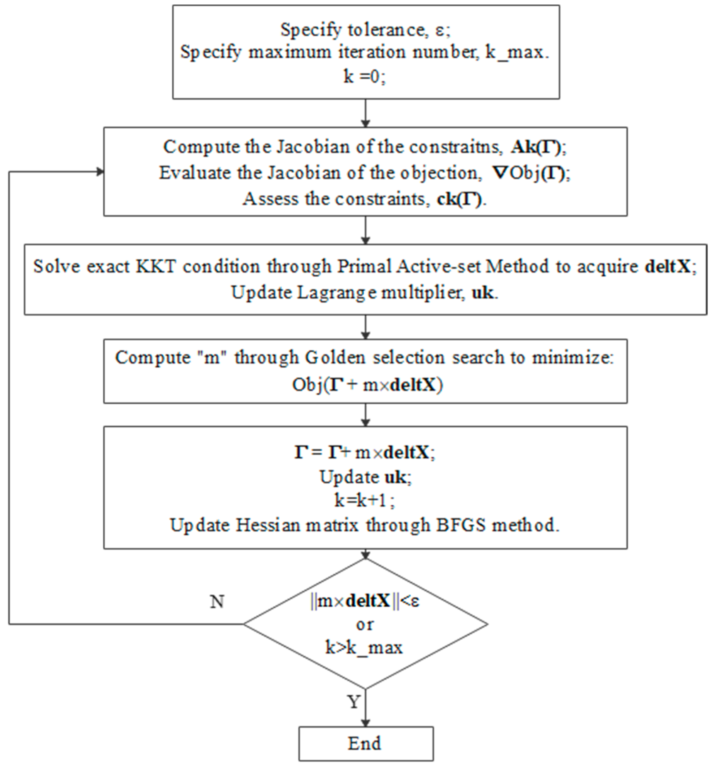
The modified SQP algorithm used in this paper is illustrated in Figure 8 [25]. One of the main calculation burdens of these gradient-based algorithms lies in acquiring the Jacobian matrix of the target $\nabla Obj\left(\mathit{\Gamma }\right)$. Conventional numerical methods that approximate derivatives by differences are usually adopted for nonlinear models, while the heavy computational burden prevents them from online realization. In addition, with parameters that have different magnitude ranges, the corresponding discretization error may be great and can lead to the divergence of the model. To solve this problem, a kind of fast calculation method for the Jacobian matrix $\nabla Obj\left(\mathit{\Gamma }\right)$ is presented, which helps alleviate the computation burden and improves the optimization efficiency.

The LPTN model prediction error can be assessed as

$$Obj\left(\mathit{\Gamma }\right)=tra\left(\left[\mathit{Y}\left(\mathit{\Gamma }\right)-{\mathit{Y}}_{\mathit{m}}\right]\mathit{W}{\left[\mathit{Y}\left(\mathit{\Gamma }\right)-{\mathit{Y}}_{\mathit{m}}\right]}^{\prime }\right)$$

(33)

where $\mathit{Y}\left(\mathit{\Gamma }\right)$ denotes the model-predicted temperature output corresponding to the parameter vector $\mathit{\Gamma }$, ${\mathit{Y}}_{\mathit{m}}$ is the measured temperature vector, and $\mathit{W}$ is the weighting matrix. The weighting matrix is introduced to assign different importance to different temperature samples, allowing recent or more reliable measurements to have stronger influence on the optimization process. Thus, $Obj\left(\mathit{\Gamma }\right)$ represents a weighted quadratic error index that quantifies the discrepancy between predicted and measured temperatures. Accordingly, the gradient of the $Obj\left(\mathit{\Gamma }\right)$ with respect to $\mathit{\Gamma }$ can be calculated through [25]

$$\nabla Obj\left(\mathit{\Gamma }\right)={\left(\mathit{v}\mathit{e}\mathit{c}\left[\left({\mathit{W}}^{\prime }+\mathit{W}\right)\left(\mathit{Y}\left(\mathit{\Gamma }\right)-{\mathit{Y}}_{\mathit{m}}\right)\right]\right)}^{\prime }\times \nabla \mathit{Y}\left(\mathit{\Gamma }\right)$$

(34)

where $\mathit{v}\mathit{e}\mathit{c}$ is an operator that transforms a matrix into a vector by stacking the columns. This expression indicates that the gradient of the objective function is determined by the sensitivity of the model output $\mathit{Y}\left(\mathit{\Gamma }\right)$ with respect to the parameter vector $\mathit{\Gamma }$. Therefore, the key task becomes the efficient computation of $\nabla \mathit{Y}\left(\mathit{\Gamma }\right)$. Based on (25)–(29), $\nabla \mathit{Y}\left(\mathit{\Gamma }\right)$ can be derived through the sensitivity propagation of the state variables. The recursive formulation is given as

$$\begin{array}{c}\nabla \mathit{T}\left(n,\mathit{\Gamma }\right)=\nabla \left({\mathit{M}}_T\left(\mathit{\Gamma }\right)\mathit{T}\left(n-1,\mathit{\Gamma }\right)\right)+\nabla \left(\left[{\mathit{M}}_P\left(\mathit{\Gamma }\right),{\mathit{M}}_U\left(\mathit{\Gamma }\right)\right]\left[\begin{array}{c}\mathit{P}\\ {\mathit{U}}_{\mathit{C}}\end{array}\right]\right)\\ =\mathit{v}\mathit{e}\mathit{c}\left[{\displaystyle \frac{\mathsf{\partial }{\mathit{M}}_T\left(\mathit{\Gamma }\right)}{\mathsf{\partial }{\mathit{x}}^{\prime }}}\mathit{T}\left(n-1,\mathit{\Gamma }\right)+{\mathit{M}}_T\left(\mathit{\Gamma }\right){\displaystyle \frac{\mathsf{\partial }\mathit{T}\left(n-1,\mathit{\Gamma }\right)}{\mathsf{\partial }{\mathit{x}}^{\prime }}}\right]+\mathit{v}\mathit{e}\mathit{c}\left[{\displaystyle \frac{\mathsf{\partial }\left[{\mathit{M}}_P\left(\mathit{\Gamma }\right),{\mathit{M}}_U\left(\mathit{\Gamma }\right)\right]}{\mathsf{\partial }{\mathit{\Gamma }}^{\prime }}}\left[\begin{array}{c}\mathit{P}\\ {\mathit{U}}_{\mathit{C}}\end{array}\right]\right]\\ =\left({\mathit{I}}_q⨂{\mathit{M}}_T\left(\mathit{\Gamma }\right)\right)\nabla \mathit{T}\left(n-1,\mathit{\Gamma }\right)+\mathit{X}\left(n-1\right)\end{array}$$

(35)

$$\nabla \mathit{Y}\left(n,\mathit{\Gamma }\right)=\nabla \left({\mathit{S}}_{\mathit{m}}\mathit{T}\left(n,\mathit{\Gamma }\right)\right)=\left({\mathit{I}}_q⨂{\mathit{S}}_{\mathit{m}}\right)\nabla \mathit{T}\left(n,\mathit{\Gamma }\right)$$

(36)

$$\mathit{X}\left(n-1\right)=\left({\left[\begin{array}{c}\mathit{T}\left(n-1,\mathit{\Gamma }\right)\\ \begin{array}{c}\mathit{P}\\ {\mathit{U}}_{\mathit{C}}\end{array}\end{array}\right]}^{\prime }⨂{\mathit{I}}_m\right)\nabla \left[{\mathit{M}}_T\left(\mathit{\Gamma }\right),{\mathit{M}}_P\left(\mathit{\Gamma }\right),{\mathit{M}}_U\left(\mathit{\Gamma }\right)\right]$$

(37)

where $\otimes$ is the Kronecker tensor product, $q$ is the column number of $\mathit{T}$, and m is the row number of $\left[{\mathit{M}}_T\left(\mathit{\Gamma }\right),{\mathit{M}}_P\left(\mathit{\Gamma }\right),{\mathit{M}}_U\left(\mathit{\Gamma }\right)\right]$. Based on the modeling process presented in Section 2, $\nabla \left[{\mathit{M}}_T\left(\mathit{\Gamma }\right),{\mathit{M}}_P\left(\mathit{\Gamma }\right),{\mathit{M}}_U\left(\mathit{\Gamma }\right)\right]$ can be calculated offline with the help of the symbol calculation technique and written in the program. It can be observed from (35) and (36) that the sensitivity propagation can also be expressed in a state-space form. In this interpretation, $\nabla \mathit{Y}\left(n,\mathit{\Gamma }\right)$ acts as the state variable describing how node temperatures change with respect to parameter variations, $\mathit{X}\left(n\right)$ serves as the input representing parameter-induced excitation, and $\nabla \mathit{T}\left(n,\mathit{\Gamma }\right)$ is the output representing the sensitivity of the measured temperatures. Thus, $\nabla \mathit{Y}\left(\mathit{\Gamma }\right)$ can be iteratively calculated through (35) and (36). Once $\nabla \mathit{Y}\left(\mathit{\Gamma }\right)$ is obtained, $\nabla Obj\left(\mathit{\Gamma }\right)$ can be computed directly from (34). With Jacobian matrix $\nabla Obj\left(\mathit{\Gamma }\right)$ determined analytically, the gradient-based optimization can be realized efficiently.

To further reduce the computational burden, the key parameters are screened before each optimization process. Based on the definition of $\nabla Obj\left(\mathit{\Gamma }\right)$, the objective function $Obj\left(\mathit{\Gamma }\right)$ can be locally approximated around the current operating point ${\mathit{\Gamma }}_0$ using a first-order expansion. This approximation provides a direct way to evaluate how each parameter variation contributes to the change in prediction error:

$$Obj\left({\mathit{\Gamma }}_0+∆\mathit{\Gamma }\right)\approx \nabla Obj\left({\mathit{\Gamma }}_0\right)∆\mathit{\Gamma }=\left[\begin{array}{cccc}{\left.{\displaystyle \frac{\partial Obj\left(\mathit{\Gamma }\right)}{\partial {\mathsf{\Gamma }}_1}}\right|}_{\mathit{\Gamma }={\mathit{\Gamma }}_0}& {\left.{\displaystyle \frac{\partial Obj\left(\mathit{\Gamma }\right)}{\partial {\mathsf{\Gamma }}_2}}\right|}_{\mathit{\Gamma }={\mathit{\Gamma }}_0}& \dots & {\left.{\displaystyle \frac{\partial Obj\left(\mathit{\Gamma }\right)}{\partial {\mathsf{\Gamma }}_n}}\right|}_{\mathit{\Gamma }={\mathit{\Gamma }}_0}\end{array}\right]\times \left[\begin{array}{c}∆{\mathsf{\Gamma }}_1\\ ∆{\mathsf{\Gamma }}_2\\ \dots \\ ∆{\mathsf{\Gamma }}_n\end{array}\right]=\sum _k\mathsf{\Lambda }\left(k\right)$$

(38)

Equation (38) shows that the variation in the objective function can be approximated as the weighted summation of the contributions from each parameter. Each term $\mathsf{\Lambda }\left(k\right)$ represents the local influence of the $k$th parameter on the prediction error when it changes by $∆{\mathsf{\Gamma }}_k$:

$$\mathsf{\Lambda }\left(k\right)={\left.{\displaystyle \frac{\partial Obj\left(\mathit{\Gamma }\right)}{\partial {\mathsf{\Gamma }}_k}}\right|}_{\mathit{\Gamma }={\mathit{\Gamma }}_0}∆{\mathsf{\Gamma }}_k$$

(39)

According to the basic idea of parameter sensitivity analysis, factor $\mathsf{\Lambda }\left(k\right)$ represents the local contribution of parameter ${\mathsf{\Gamma }}_k$ to the variation in the objective function when it changes by $∆{\Gamma }_k$. In other words, $\mathsf{\Lambda }\left(k\right)$ quantifies how strongly a small adjustment of a specific parameter influences the prediction error around the current operating point ${\mathit{\Gamma }}_0$. A larger absolute value of $\mathsf{\Lambda }\left(k\right)$ indicates that the corresponding parameter has a stronger impact on the objective function and is therefore more relevant for optimization. Thus, within the limitation [$L_k,U_k]$, the impact of manipulating ${\mathsf{\Gamma }}_k$ can be assessed through

$$o\left({\mathsf{\Gamma }}_k\right)=\mathrm{m}\mathrm{a}\mathrm{x}\left\{\mathsf{\Lambda }\left(k\right)\left({\displaystyle \frac{{\mathsf{\Gamma }}_k-L_k}{Z}}\right),\mathsf{\Lambda }\left(k\right)\left({\displaystyle \frac{{\mathsf{\Gamma }}_k-U_k}{Z}}\right),0\right\}$$

(40)

where $Z$ is a constant scaling factor. When $\mathsf{\Lambda }\left(k\right)$ is positive, decreasing ${\mathsf{\Gamma }}_k$ can reduce the value of $Obj\left(\mathit{\Gamma }\right)$. When Λ(k) is negative, an increase in ${\mathsf{\Gamma }}_k$ leads to a reduction in $Obj\left(\mathit{\Gamma }\right)$. So, $o\left({\mathsf{\Gamma }}_k\right)$ can be interpreted as a practical optimization potential index that measures the ability of parameter ${\mathsf{\Gamma }}_k$ to reduce the objective function within its allowable constraint range [$L_k,U_k]$. Thus, the parameters that have larger $o\left({\mathsf{\Gamma }}_k\right)$ are expected to possess stronger potential in reducing the prediction error and are selected as the key parameters to be tuned in the following optimization algorithm. This parameter screening process allows the optimization to focus only on the most influential parameters, which significantly reduces the computational burden and improves efficiency for online implementation. It is worth pointing out that this parameter selection procedure is repeated before every optimization calculation to ensure that the most relevant parameters are always identified under changing operating conditions.

With the derived calculation method of $\nabla Obj\left(\mathit{\Gamma }\right)$ and the parameter selection process, the LPTN model parameters can be optimized efficiently online. The effectiveness of the proposed method will be demonstrated in the following section.

5. Experimental Assessment

5.1. The Verification of the Proposed Method

The experiments here are processed to verify the proposed method under the condition that the machine’s thermal features are varied from the pre-established LPTN model. In practice, modifying the thermal performance of the real machine is difficult, so the LPTN model parameters are intentionally changed to enlarge the prediction error.

To emphasize latest measured results, the weighting matrix is adopted as

$$\mathit{W}=diag\left({\displaystyle \frac{1-e^{-\frac{1}{F\times N}}}{1-e^{-\frac{1}{F}}}},{\displaystyle \frac{1-e^{-\frac{2}{F\times N}}}{1-e^{-\frac{1}{F}}}},\dots ,{\displaystyle \frac{1-e^{-\frac{N}{F\times N}}}{1-e^{-\frac{1}{F}}}}\right)$$

(41)

where $N$ is the length of the data and $F$ is a constant, adopted as 0.05 in this paper. The $T_s$ shown in Figure 7 is set as 3 min.

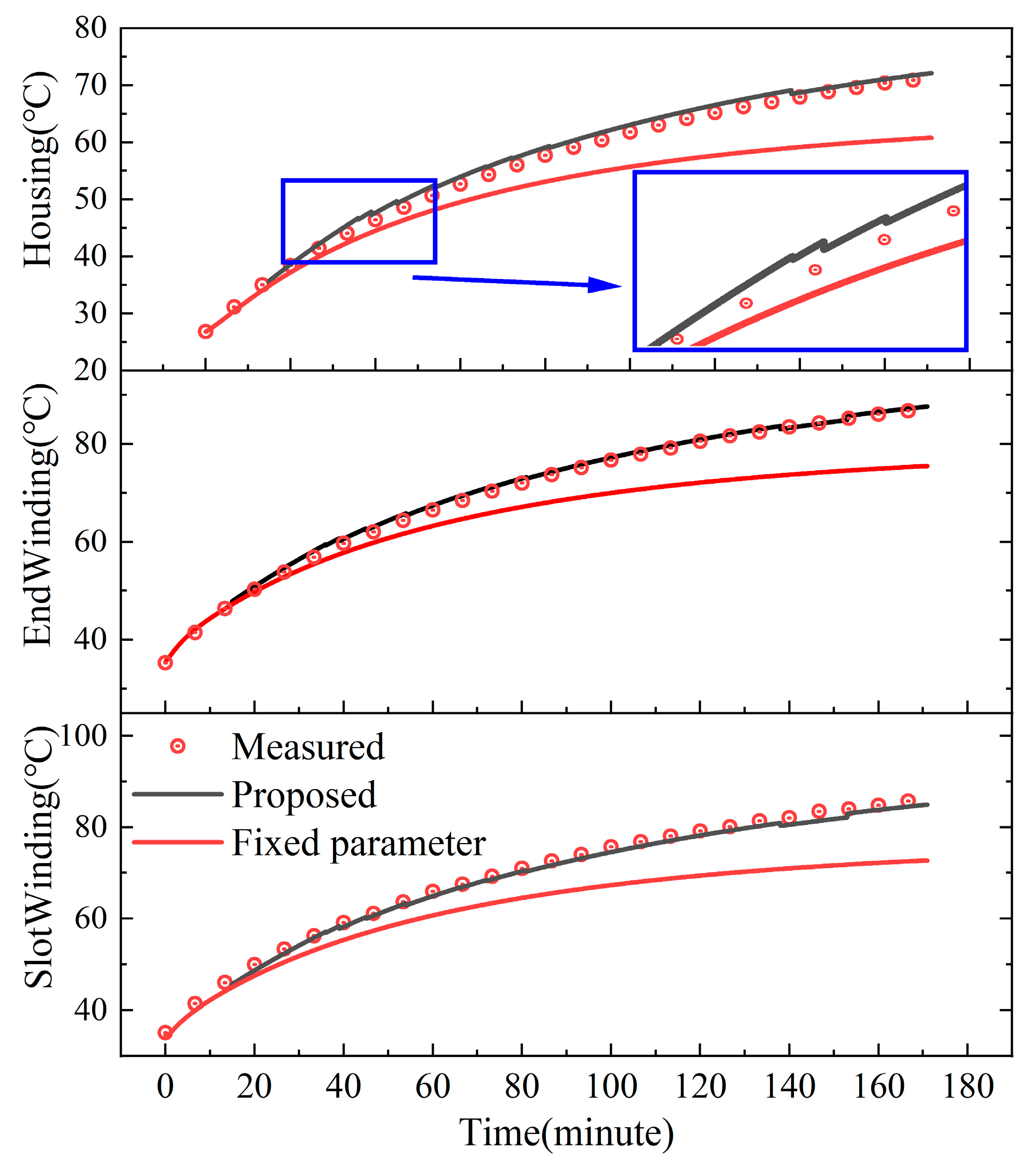
First, the parameter-tracking ability of the proposed method is assessed. The thermal resistance between housing and environment $R_{e\_hous}$ is reduced from 9.1 °C/W to 6.1 °C/W, while all the other parameters are identical with those estimated in Section 3. For this case, the parameter to optimize is fixed as $R_{e\_hous}$. The performance of the proposed method under the working condition of 600 rpm 70 Nm is shown in Figure 9.

It can be seen that the prediction error of the LPTN model with the fixed parameters is obvious. On the other hand, the proposed method adaptively updates the model and successfully limits the error. The enlarged part shown in Figure 9 suggests that with the accumulation of the measured data, the model output is gradually improved. It should be pointed out that the parameter estimation and the temperature prediction process are all based on historical data. In other words, at time $k{T}_s$, the parameter estimation is based on the measured results during $0~k{T}_s$. After this, the latest LPTN model outputs the predicted results for time $k{T}_s~(k+1)T_s$.

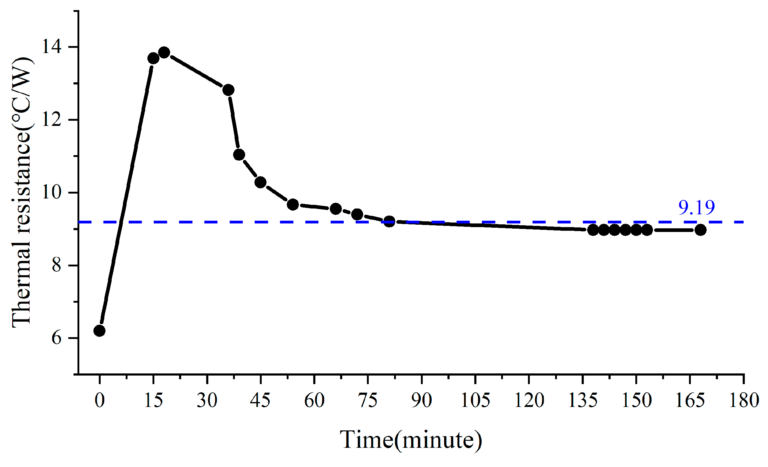
The variation of $R_{e\_hous}$ during the adaptation process is shown in Figure 10. It can be seen from Figure 9 and Figure 10 that the initial value of $R_{e\_hous}$ is smaller than the offline estimated result. So, at first, the predicted temperatures are lower than the measured results. Thus, the proposed adaptive method first increases the parameter. However, the modified value is overlarge, and the predicted temperatures become higher than the measured data, as shown in the enlarged part in Figure 9. Along with the accumulation of the measured data, the proposed method gradually reduces the parameter. Finally, $R_{e\_hous}$ is maintained at about 8.96 °C/W which is close to the offline estimated value 9.19 °C/W.

To further assess the performance of the proposed method, the experiment under the condition of multiple parameters having been varied is processed. For electrical machines, the stator and rotor core-related thermal parameters are relatively stable. The variation parts are mainly related to the winding and housing-environment. Considering this, the variables of the LPTN thermal parameters were chosen as the 14 parameters related to thermal conductivity, thermal resistance, and thermal capacitance of the housing-environment, slot winding, and end winding. Thus, the dimension of $\mathit{\Gamma }$ is 14. And the selected $k$ parameters are those that have the largest $o\left({\mathsf{\Gamma }}_k\right)$ and satisfy

$$\sum _{i=1}^{k}o\left({\mathsf{\Gamma }}_i\right)\ge 0.98\sum _{i}o\left(x_i\right)\ge \sum _{i=1}^{k-1}o\left({\mathsf{\Gamma }}_i\right)$$

(42)

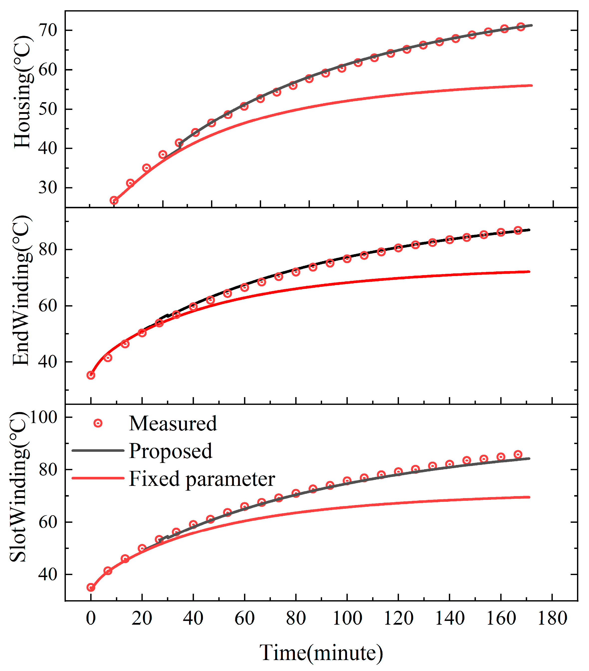
The variation in the LPTN parameters in this experiment is tabulated in

Table 4. The initial parameter variation.

Parameter	Variation
Radial thermal conductivity of slot winding	$-4\mathrm{W}/(\mathrm{m}°\mathrm{C})$
Circumferential thermal conductivity of slot winding	$-1.5\mathrm{W}/(\mathrm{m}°\mathrm{C})$
Thermal capacitance of slot winding	$-50\mathrm{J}/(\mathrm{k}\mathrm{g}°\mathrm{C})$
Thermal resistance of housing-environment	$-4°\mathrm{C}/\mathrm{W}$

, and the performance of the proposed method under this condition is illustrated in Figure 11. It can be seen from Figure 11 that the proposed method can also achieve decent results in this process. The precision of the model output is adaptively improved. It is worth pointing out that, as the model outputs hold a nonlinear relationship with the model parameters, multiple model parameters cannot be uniquely determined based on limited measured data. In other words, the estimated parameters may not converge to the corresponding offline estimated value. However, these parameters can also drive model output to match corresponding measured results; thus, the precision of the model output is increased.

5.2. The Comparison with the Numerical and EKF Method

To evaluate the properties of the proposed method, the comparison with the numerical method is processed. The numerical SQP method is realized through the fmincon tool embedded in Matlab. The initial LPTN model parameters are the same as those presented in Table 4. The calculation was processed based on the whole experimental data and the maximum iteration number is three. The time consumption and the precision of the model output under the estimated parameters are compared in

Table 5. The comparison between proposed method and numerical method.

Method	Time Consumption	Variation
Proposed	$107\mathrm{s}$	$1.6°\mathrm{C}$
Numerical	$459\mathrm{s}$	$7.6°\mathrm{C}$

.

It can be seen that with more accurate and quickly calculated Jacobian matrixes, the proposed method can be realized more efficiently and achieve more precise results.

Another widely used online adaptive method for nonlinear models is EKF. As mentioned in Section 1, the EKF method puts parameters that need to be estimated into model states. Thus, based on (25)–(29), the model for EKF can be written as

$$\left\{\begin{array}{c}\mathit{L}\left(n+1\right)=\mathit{f}\left(\mathit{L}\left(n\right)\right)\\ \mathit{Y}\left(n\right)={\mathit{S}}_{\mathit{m}}\mathit{T}\left(n\right)\end{array}\right.$$

(43)

where

$$\mathit{L}\left(n\right)=\left[\begin{array}{c}\mathit{T}\left(n\right)\\ \mathit{\Gamma }\end{array}\right]$$

(44)

$$\mathit{f}\left(\mathit{L}\left(n\right)\right)=\left[\begin{array}{c}{\mathit{M}}_P\left(\mathit{\Gamma }\right)\mathit{P}+{\mathit{M}}_T\left(\mathit{\Gamma }\right)\mathit{T}\left(n\right)+{\mathit{M}}_U\left(\mathit{\Gamma }\right){\mathit{U}}_C\\ \mathit{\Gamma }\end{array}\right]$$

(45)

The corresponding Jacobian matrix of f with respect to state L can be written as

$$\nabla \mathit{f}={\displaystyle \frac{\mathsf{\partial }\left[\begin{array}{c}{\mathit{M}}_P\left(\mathit{\Gamma }\right)\mathit{P}+{\mathit{M}}_T\left(\mathit{\Gamma }\right)\mathit{T}+{\mathit{M}}_U\left(\mathit{\Gamma }\right){\mathit{U}}_C\\ \mathit{x}\end{array}\right]}{\mathsf{\partial }\left[\mathit{T},\mathit{\Gamma }\right]}}=\left[\begin{array}{cc}{\mathit{M}}_T\left(\mathit{\Gamma }\right)& \mathsf{\partial }\mathit{T}\\ \mathbf{0}& \mathit{E}\end{array}\right]$$

(46)

where the Jacobian matrix $\nabla \mathit{T}$ can also be calculated based on the proposed method (35).

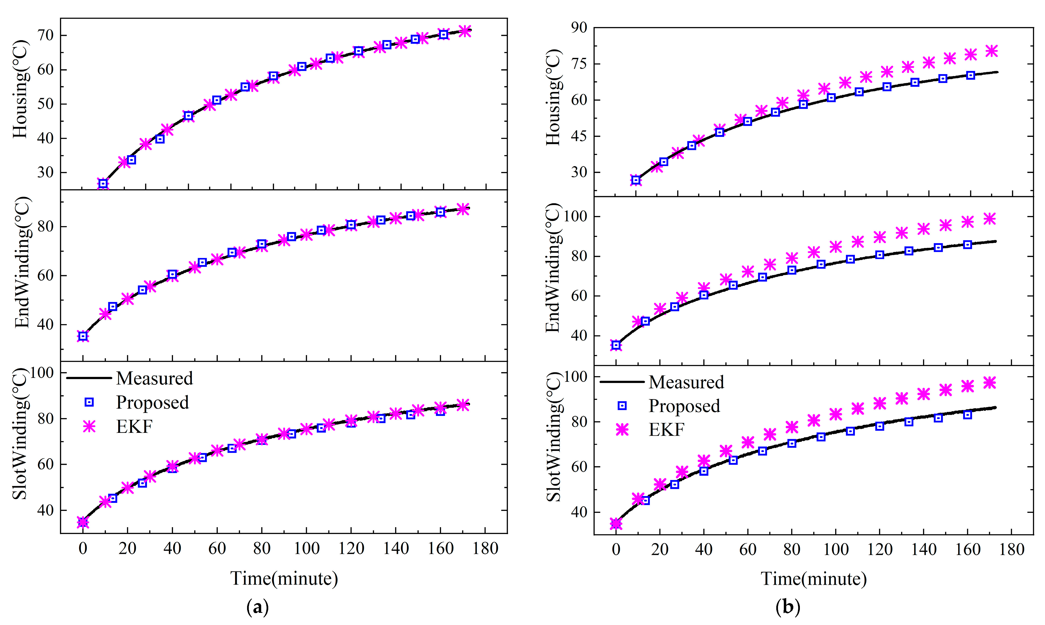
The performance of the EKF and the proposed method is compared in Figure 12. The initial LPTN model parameters were still the same as those given in Table 4. The EKF was processed every minute.

It is clear from Figure 12a that with proper temperature feedback, both methods can adaptively improve the LPTN model output and reduce the prediction error. The performance of the LPTN model with the parameters tuned through the EKF and the proposed method is illustrated in Figure 12b. It can be seen that the model parameters obtained through the EKF method can still lead to biased results; the average prediction error is about 11.9 °C, whereas the prediction error for the LPTN model with the parameters obtained through the proposed method is about 2.3 °C. This confirms that as the EKF realizes model output improvement through modifying $\mathit{L}\left(n\right)$, i.e., both $\mathit{T}\left(n\right)$ and $\mathit{\Gamma }$, even when the model output is precise, the estimated $\mathit{\Gamma }$ may still be inappropriate. Thus, compared to the EKF, the proposed method is more suitable for online model parameter estimation purposes.

Based on the comparisons made above, it can be concluded that the proposed method is computationally efficient and can realize the model parameter estimation effectively online.

6. Conclusions

In this paper, a PM machine LPTN model and online parameter estimation technique were integrated. The key point lies in reducing the calculation burden of the Jacobian matrix and enabling online realization.

Once the model prediction error exceeds the threshold, the LPTN thermal parameters are estimated and updated through the gradient-based optimization method SQP. Based on the basic structure of the LPTN model, a fast-calculation method for the Jacobian matrix of the prediction error was proposed. Thus, the conventional numerical calculation is avoided, and the corresponding calculation burden is alleviated. This enables the online realization of the gradient-based optimization method.

The proposed method is verified based on a 10 kW PM machine. And the comparison with the widely used numerical method demonstrates that the proposed method can be realized more efficiently and acquire more accurate results. On the other hand, compared to the EKF method, the parameters tuned through the proposed method can lead to a more precise model. Thus, it can be concluded that the proposed method can be realized efficiently online and is suitable for online LPTN model adaptation purposes.

References

1. Sciascera, C.; Giangrande, P.; Papini, L.; Gerada, C.; Galea, M. Analytical Thermal Model for Fast Stator Winding Temperature Prediction. IEEE Trans. Ind. Electron. 2017, 64, 6116–6126. [Google Scholar] [CrossRef]
2. Hey, J.; Malloy, A.C.; Martinez-Botas, R.; Lamperth, M. Online Monitoring of Electromagnetic Losses in an Electric Motor Indirectly Through Temperature Measurement. IEEE Trans. Energy Convers. 2016, 31, 1347–1355. [Google Scholar] [CrossRef]
3. Boglietti, A.; Cossale, M.; Vaschetto, S.; Dutra, T. Winding Thermal Model for Short-Time Transient: Experimental Validation in Operative Conditions. IEEE Trans. Ind. Appl. 2018, 54, 1312–1319. [Google Scholar] [CrossRef]
4. Boglietti, A.; Carpaneto, E.; Cossale, M.; Vaschetto, S. Stator-Winding Thermal Models for Short-Time Thermal Transients: Definition and Validation. IEEE Trans. Ind. Electron. 2016, 63, 2713–2721. [Google Scholar] [CrossRef]
5. Zhang, H.; Giangrande, P.; Sala, G.; Xu, Z.; Hua, W.; Madonna, V.; Gerada, D.; Gerada, C. Thermal Model Approach to Multisector Three-Phase Electrical Machines. IEEE Trans. Ind. Electron. 2021, 68, 2919–2930. [Google Scholar] [CrossRef]
6. Shams, G.P.; Kallaste, A.; Belahcen, A.; Vaimann, T. Analytical Thermal Model and Flow Network Analysis Suitable for Open Self-Ventilated Machines. IET Electr. Power Appl. 2020, 14, 929–936. [Google Scholar] [CrossRef]
7. Petrov, I.; Lindh, P.; Niemela, M.; Scherman, E.; Wallmark, O.; Pyrhonen, J. Investigation of a Direct Liquid Cooling System in a Permanent Magnet Synchronous Machine. IEEE Trans. Energy Convers. 2020, 35, 808–817. [Google Scholar] [CrossRef]
8. Boglietti, A.; Cavagnino, A.; Staton, D.; Shanel, M.; Mueller, M.; Mejuto, C. Evolution and Modern Approaches for Thermal Analysis of Electrical Machines. IEEE Trans. Ind. Electron. 2009, 56, 871–882. [Google Scholar] [CrossRef]
9. Dong, T.; Zhang, X.; Zhu, C.; Zhou, F.; Sun, Z. Improved Thermal Modeling Methodology for Embedded Real-Time Thermal Management System of Automotive Electric Machines. IEEE Trans. Ind. Inf. 2021, 17, 4702–4713. [Google Scholar] [CrossRef]
10. Yang, Y.; Bilgin, B.; Kasprzak, M.; Nalakath, S.; Sadek, H.; Preindl, M.; Cotton, J.; Schofield, N.; Emadi, A. Thermal Management of Electric Machines. IET Electr. Syst. Transp. 2017, 7, 104–116. [Google Scholar] [CrossRef]
11. Oyvang, T.; Noland, J.K.; Hegglid, G.J.; Lie, B. Online Model-Based Thermal Prediction for Flexible Control of an Air-Cooled Hydrogenerator. IEEE Trans. Ind. Electron. 2019, 66, 6311–6320. [Google Scholar] [CrossRef]
12. Qi, F.; Stippich, A.; Ralev, I.; Klein-Hessling, A.; de Doncker, R.W. Model Predictive Control of a Switched Reluctance Machine for Guaranteed Overload Torque. IEEE Trans. Ind. Appl. 2019, 55, 1321–1331. [Google Scholar] [CrossRef]
13. Dong, X.; Griffo, A.; Hewitt, D.; Wang, J. Reduced-Order Thermal Observer for Power Modules Temperature Estimation. IEEE Trans. Ind. Electron. 2020, 67, 10085–10094. [Google Scholar] [CrossRef]
14. van der Broeck, C.H.; Lorenz, R.D.; de Doncker, R.W. Monitoring 3-D Temperature Distributions and Device Losses in Power Electronic Modules. IEEE Trans. Power Electron. 2019, 34, 7983–7995. [Google Scholar] [CrossRef]
15. Boglietti, A.; Cossale, M.; Popescu, M.; Staton, D.A. Electrical Machines Thermal Model: Advanced Calibration Techniques. IEEE Trans. Ind. Appl. 2019, 55, 2620–2628. [Google Scholar] [CrossRef]
16. Wallscheid, O.; Böcker, J. Global Identification of a Low-Order Lumped-Parameter Thermal Network for Permanent Magnet Synchronous Motors. IEEE Trans. Energy Convers. 2016, 31, 354–365. [Google Scholar] [CrossRef]
17. Madonna, V.; Giangrande, P.; Galea, M. Influence of Insulation Thermal Aging on the Temperature Assessment in Electrical Machines. IEEE Trans. Energy Convers. 2021, 36, 456–467. [Google Scholar] [CrossRef]
18. Yang, H.; Ni, J. Adaptive model estimation of machine-tool thermal errors based on recursive dynamic modeling strategy. Int. J. Mach. Tools Manuf. 2005, 45, 1–11. [Google Scholar] [CrossRef]
19. Erazo, D.E.G.; Wallscheid, O.; Bocker, J. Improved Fusion of Permanent Magnet Temperature Estimation Techniques for Synchronous Motors Using a Kalman Filter. IEEE Trans. Ind. Electron. 2020, 67, 1708–1717. [Google Scholar] [CrossRef]
20. Shi, W.; Zhou, X. Online Estimation Method for Permanent Magnet Temperature of High-Density Permanent Magnet Synchronous Motor. IEEJ Trans. Electr. Electron. Eng. 2020, 15, 751–756. [Google Scholar] [CrossRef]
21. Xiao, S.; Griffo, A. Online Thermal Parameter Identification for Permanent Magnet Synchronous Machines. IET Electr. Power Appl. 2020, 14, 2340–2347. [Google Scholar] [CrossRef]
22. Sheng, Z.; Wang, D.; Fu, J.; Hu, J. A Computationally Efficient Spatial Online Temperature Prediction Method for PM Machines. IEEE Trans. Ind. Electron. 2022, 69, 10904–10914. [Google Scholar] [CrossRef]
23. Jiang, S.; Zhou, B.; Huang, X.; Wang, K.; Xu, L. 3-D Global Thermal Analysis of DSEM Considering the Temperature Difference Between Excitation and Armature Coils. IEEE Trans. Ind. Electron. 2021, 68, 11931–11940. [Google Scholar] [CrossRef]
24. Liang, D.; Zhu, Z.Q.; Zhang, Y.; Feng, J.; Guo, S.; Li, Y.; Wu, J.; Zhao, A. A Hybrid Lumped-Parameter and Two-Dimensional Analytical Thermal Model for Electrical Machines. IEEE Trans. Ind. Appl. 2021, 57, 246–258. [Google Scholar] [CrossRef]
25. Antoniou, A.; Lu, W. Practical Optimization: Algorithms and Engineering Applications; Springer: New York, NY, USA, 2007. [Google Scholar]
Figure 1. The three-dimensional LPTN model. (a) Axial view; (b) one piece of radial view.
Energies 19 01031 g001
Figure 2. The basic arc component and corresponding T model. (a) Basic cylindrical element; (b) three-dimensional T model.
Energies 19 01031 g002
Figure 3. PT100 distribution.
Energies 19 01031 g003
Figure 4. The topology of the test machine.
Energies 19 01031 g004
Figure 5. Experimental setup.
Energies 19 01031 g005
Figure 6. The performance of the offline estimated parameters under different working conditions.
Energies 19 01031 g006
Figure 7. The LPTN model adaptation process.
Energies 19 01031 g007
Figure 8. The calculation process of the modified SQP optimization algorithm.
Energies 19 01031 g008
Figure 9. The performance of the proposed adaptive method.
Energies 19 01031 g009
Figure 10. The adaptation of R e _ h o u s through the proposed method.
Energies 19 01031 g010
Figure 11. The performance of the proposed method under the condition that multiple parameters have been varied.
Energies 19 01031 g011
Figure 12. The comparison between the proposed method and EKF. (a) Online performance; (b) performance of estimated parameters.
Energies 19 01031 g012