Article

The Impact of Electric Vehicle Hosting Factors on Distribution Network Performance Using an Impedance-Based Heuristic Approach


by
Abdullah Alrashidi
1,*,
Nora Elayaat
2,
Adel A. Abou El-Ela
3,
Ashraf Fahmy
1,4,
Ismail Hafez
5,
Tamer Attia
3 and
Abdelazim Salem
2
1
Faculty of Science and Engineering, Swansea University, Swansea SA1 8EN, UK
2
Department of Electrical Engineering, College of Engineering, October 6 University, 6th of October City, Giza 12585, Egypt
3
Electrical Engineering Department, Faculty of Engineering, Menofia University, Shebin El-Kom 32511, Egypt
4
Electrical Power and Machines Department, Capital University (Formerly: Helwan University), Cairo 11795, Egypt
5
Electronics and Electrical Communication Department, College of Engineering, Ain Shams University, Cairo 11517, Egypt
*
Author to whom correspondence should be addressed.
Energies 2026, 19(3), 753; https://doi.org/10.3390/en19030753
Submission received: 23 December 2025 / Revised: 21 January 2026 / Accepted: 24 January 2026 / Published: 30 January 2026

Abstract

The fast adoption of electric vehicles (EVs) and the integration of renewable distributed generators (DGs) provide significant operational issues for radial distribution networks (RDNs), notably in terms of power losses, voltage variations, and system stability. This paper investigates the optimal placement and sizing of EV charging stations (EVCSs) and DGs under varying EV hosting factors (EV-HFs). An impedance matrix-based load flow method is developed, and a derived analytical formula for power loss calculation is proposed to improve computational efficiency. A weighted multi-objective function is developed to reduce active power losses and voltage variations while optimizing the voltage stability index and the yearly cost savings from energy loss. The optimization is performed using a deterministic heuristic procedure that incrementally adjusts the location and size of EVCSs and DGs until no further improvement in the fitness function is achieved. This stepwise approach provides fast convergence with low computational effort compared to population-based metaheuristics. The methodology is used on the IEEE 33-bus system under different loading conditions and EV-HFs. The results reveal that for 40% and 60% EV-HFs, active power losses decreased by about 57% compared with the basic case, while the minimum bus voltage improved from 0.9148 pu to 0.9654 pu and 0.9641 pu. The economic analysis demonstrates annual savings of up to USD 473,550, with a payback period between 7 and 8 years. These findings emphasize the need of integrated EVCS and DG planning in improving future distribution systems’ technical and economic performance.

1. Introduction

The growing utilization of electric vehicles (EVs) necessitates the integration of electric vehicle charging stations (EVCSs) into distribution networks. However, this integration introduces significant challenges, as it increases network loading, which in turn raises power losses and voltage drops along distribution branches, thereby reducing voltage levels. Previous studies have carefully explored the optimal location of EVCSs from an operational standpoint, considering factors such as waiting time, driving range, customer satisfaction, and market size [1]. Other studies have focused on decreasing power losses and voltage variations while including the idea of hosting factors (HFs), with specific emphasis on EV hosting factors [2,3]. This underscores the importance of further exploring the relationship between EV demand load and network performance.
A previous study aimed to reduce active and reactive power losses for various EV-HF values. The Quantum-Behaved Gaussian Mutational Dragonfly Algorithm (QGDA) was used for optimization [4], while Harmony Particle Swarm Optimization (PSO) improved voltage quality [5]. Additional research has explored the integration of EVCSs with other network components, such as distributed generators (DGs) and DSTATCOMs, to enhance efficiency and reliability [6,7,8]. Despite these efforts, the restricted treatment of EV-HFs prevents a thorough evaluation of such treatments. A prominent research trend is the cooperative optimization of power losses in networks that concurrently host both EVCSs and DGs [7,8]. Approaches have included hybrid artificial intelligence techniques combining Grey Wolf Optimizer with PSO, Modified Teaching–Learning-Based Optimization (TLBO), and Multi-Objective PSO (MOPSO). However, these studies frequently lack a thorough examination of the interplay between hosting factors and network performance, resulting in a large research gap.
Several studies have studied how to reduce energy losses and voltage variations using different optimization methodologies, such as Differential Evolution (DE), Grey Wolf Optimizer (GWO), adaptive Particle Swarm Optimization (PSO), and the Fuzzy Analytic Hierarchy Process (AHP) [9,10]. In ref. [11], the EV hosting factor (EV-HF) was supposed to be the whole demand load. Ref. [12] presents a detailed evaluation of ideal EVCS placement, taking into account different objectives, solution approaches, and geographic factors for enhancing charging infrastructure design in smart grids. In comparison, some studies have addressed uncertainties in EV-HFs using probabilistic modeling [13,14], while some studies have studied the use of renewable energy sources at charging stations to minimize grid demand [15]. This calls into doubt the applicability of standard EV-HF-based models in scenarios with significant renewable penetration. Optimization techniques such as GWO-PSO hybrids [13,15], Chicken Swarm Optimization (CSO), TLBO [16], and combined Lazy Greedy algorithms (Direct Gain and Effective Gain, LGEG) [17] have also been used to reduce power loss and voltage variations.
In addition, various mathematical and metaheuristic strategies have been employed for optimal EVCS placement with the aim of improving efficiency and reliability. Examples are Mixed Integer Nonlinear Programming (MINLP) [18], DE coupled with Harris Hawks Optimization (DE-HHO) [19], the Binary Atom Search method [20], and the BAT algorithm [21]. However, many of these methodologies frequently miss the effect of renewable distributed generation hosting factors (RDG-HFs), restricting their optimization reach. It is also noteworthy that the EV-HF was typically reported in discrete increments of 5%, 10%, 15%, or 20% [21]. While energy storage technologies are widely known for their capacity to reduce renewable unpredictability and supply–demand mismatches [22], the current study uses a strong optimization framework to maintain grid stability without depending on storage systems. The proposed method suggests that the optimal integration of EVCSs and PV production can significantly enhance grid performance in stochastic operating conditions. Its resilience ensures successful operation even without storage, giving a significant viewpoint for future grid integration difficulties. Future research might expand on this architecture by introducing storage systems to give greater optimization and flexibility. Meanwhile, several studies have identified differences in EV-HF distribution and their influence on network performance [23,24,25]. Also, TD3-CO-PI EMS offered a passenger-aware collaborative EMS to improve the operating efficiency of FCBs during hot weather, which improved hydrogen utilization and onboard energy system durability [26].
Recently, there has been a growing interest in the effect of wireless power transfer technology. Notably, various intelligent techniques have been highlighted in [27,28]. In [27], a new concept of the integrated inductive–capacitive core (IICC) structure, which uses the high conductivity characteristics of nanocrystalline materials and the distinctive laminated configuration of the nanocrystalline core, was used to build the resonant capacitor required in an LC resonant tank. For instance, in [28], a magnetic coupler made up of a flux pipe power supply rail and an H-type receiver is proposed to achieve the benefits of the magnetic couplers. Winding the rail coil unidirectionally in the traveling direction produces a reasonably uniform magnetic field in the traveling direction, which replaces the typical alternating magnetic field in the vertical direction.
Previous research’s shortcomings are mentioned below: Much of the previous research focused solely on the influence of RDGs, with little consideration for the significance of EV loads. While several studies have looked at the impact of EV loads, they usually disregard the hosting factor, instead portraying EV loads as a simple count of automobiles in the distribution network.
But in this manuscript, due to the different nature of loads on the RDNs, the consumed powers on the network are changed for each hour of the day; consequently, the EVs’ loadings on the network must be changed so the hosting factor of EVCSs is taken into account for this condition. The optimal selection of the placement and sizing of both EVCSs and DGs is determined at the maximum loading hour, and these placements are fixed for other hours, but the sizing of EVCSs and DGs is changed according to the loading condition at any other loading hour.
The contributions to the study are summarized as follows:
  • Development of an impedance matrix-based load flow method using the DSB incidence matrix, providing a faster and computationally efficient alternative to traditional backward/forward sweep methods for RDN analysis.
  • Development of a weighted multi-objective optimization model that balances power loss reduction, voltage deviation minimization, voltage stability enhancement, and economic advantages.
  • Introduction of a deterministic heuristic optimization procedure for the placement and sizing of EVCSs and DGs, which incrementally improves the fitness function with low computational cost.
  • Comprehensive case study on the IEEE 33-bus distribution system, showing that at 40% and 60% EV hosting factors, power losses can be reduced by ~57%, with significant improvements in voltage stability and annual economic savings.
  • Techno-economic insights for system operators, including payback periods and lifetime profit analysis, demonstrating the practical feasibility of coordinated EVCS and DG planning.

2. Problem Formulation

The proposed problem formulation considers the hourly load variations and different EV-HF scenarios, with a focus on decreasing active and reactive power losses and improving the voltage stability index. The formulation integrates technical constraints, economic considerations, and a multi-objective optimization model, as described below.

2.1. Hosting Factor of EVCSs

The HF can be defined as the capability of a distribution network to accommodate additional EVCS load without violating operational constraints such as voltage limits, thermal ratings, or stability margins. It is expressed as the ratio between the allowable EV demand load power and the total system demand power as mentioned in Equation (1), which represents the simple form used to calculate it. HF is normally calculated using a set of technical factors that vary depending on the grid being analyzed.
P EVCS = H F × P demand
Due to changing the capacities of the EVCSs, there are also varying effective ratings of DGs. Since EVCS ratings vary dynamically with the hourly load profile, the hosting factor directly influences the required DG capacities to maintain network performance. Given that the added loads actually increase the loading on the distribution branches, the thermal loading on some branches increases and the voltage drops on these branches also increase; consequently, the voltage at some buses is less than the base case. This only happens in the case of adding loads. However, the network is equipped with distributed generators that supply electric power to all distribution network loads so that the system performance is improved, which means that the branch currents are reduced and the minimum voltage on the network is increased; this means that the voltage profile on network buses is improved and the electrical losses on network can be minimized.

2.2. Economic Modeling of PV-Based DGs

PV generators are assumed to have energy storage batteries to make the system able to supply electric power to electrical distribution networks at any time and EV charging station demands are modeled as constant load power each hour based on the electric vehicle hosting factor (EV-HF) that is used for planning-stage analysis.
The cost of deploying PV-based DGs includes several components, such as solar modules, inverters, balance-of-system (BOS) costs, labor, overhead, and interconnection. The total cost of PV (PV Total_Cost) can be expressed as [29]
PVTotal _ Cos = CPV / W × PVsize
where CPV/W is the total cost of PV per watt and PVsize is the size of the PV.
Annual cost saving of energy loss:
ACSEL   =   K E × i = 1 24 P l o s s e s   o f   b a s e P l o s s e s   w i t h   D G × 365
where K E = 0.06 USD/Kwhr.

2.3. System Constraints

Some technical requirements must be verified in RDNs, which are divided into three categories: power balancing, voltage restrictions, and DG actual power constraints. The RDG’s placement is an important factor in the RDN’s power equations.

2.3.1. Power Balance Constraint

The total power generated from the slack bus and DG units must balance the system load, EVCS demand, and network losses:
P S + P D G = i = 1 N b P d e m a n d , i + P E V C S + P l o s s  
where N b is the bus number; P S   is the active power generated at the slack bus bar; P d e m a n d , i is the total active power of the load at bus (i); P E V C S is the total active power of the EVCS; and P l o s s is the total active power loss.

2.3.2. Voltage Limit

Bus voltages must remain within specified limits to ensure reliable system operation:
0.95 V i 1.05   p u
The voltage at all buses must be in the acceptable range when connecting both EVCSs and DGs, which occurs by selecting the optimal sizing and placement of them. Given that the voltage drop on each distribution branch depends on the current flow in this branch, if this current is reduced, then the voltage drop decreases. But this current has two components: the real part that depends on the active power flow and the imaginary part that is related to reactive power flow. So if the active power flow is reduced using DGs, then the voltage drop reduces; consequently, the voltage level at all buses is enhanced and the electrical losses are minimized.
The DG must guarantee that the power injected at each optimized bus is within the minimum and maximum limits.

2.3.3. DG Capacity Limits

It should fall between the minimum ( P m i n   _ D G ) and maximum ( P m a x D G ). The DG ratings are constrained to lie within minimum and maximum operating limits [25]
P m i n   _ D G P s i z e D G P m a x D G

2.4. Multi-Objective Optimization Model

The objective of this study is to find optimal locations and sizes of EVCSs and DGs such that system performance is enhanced under different EV-HFs. The optimization problem simultaneously (i) minimizes active power loss (Ploss); (ii) minimizes the voltage deviation index (VDI); (iii) maximizes the voltage stability index (VSI); and (iv) maximizes the annual cost saving of energy loss (ACSEL). These are combined into a weighted multi-objective function:
Ft = w1 Ploss + w2 VDI + w3 (1/VSI) + w4 (1/ACSEL)
where VSI (new operating condition) > VSI base case and where w1, w2, w3, and w4 are the weights assigned to each objective.
The values of them are as follows: w1 = 0.45, w2 = 0.25, w3 = 0.1, and w4 = 0.2. These values are used for normalization and sensitivity analysis for the impact of each one on the overall objective function.
The optimization model aims to determine the optimal sizing and locations for both EV charging stations and distributed generators. The optimal solution depends on minimizing the electrical power/energy losses and the voltage deviation index and increasing the voltage stability index for the electrical distribution network.

2.4.1. Power Loss

The unique technique focuses mostly on reducing P l o s s and voltage profile by properly allocating DGs and electric vehicle charging stations (EVCSs) inside the RDN to achieve the best performance. The overall real P l o s s can be expressed as
P l o s s = h = 1 24 P l o s s ( h )   and   Q l o s s = h = 1 24 Q l o s s ( h )
P l o s s ( h ) = r e a l { [ I d e m ( h )   ] * T   Z b u s   I d e m ( h ) }
Q l o s s ( h ) = i m a j { [ I d e m ( h )   ] * T   Z b u s   I d e m ( h ) }

2.4.2. Voltage Deviation Index (VDI)

Voltage deviation is the difference between the nominal voltage (which equals 1 pu) and the actual bus voltage. The system’s voltage condition improves when the bus voltage approaches the nominal value. The VDI computation may be accomplished as [30]
V D I = i N 1 V i 2
where V i is the voltage at the ith node.

2.4.3. Voltage Stability Index (VSI)

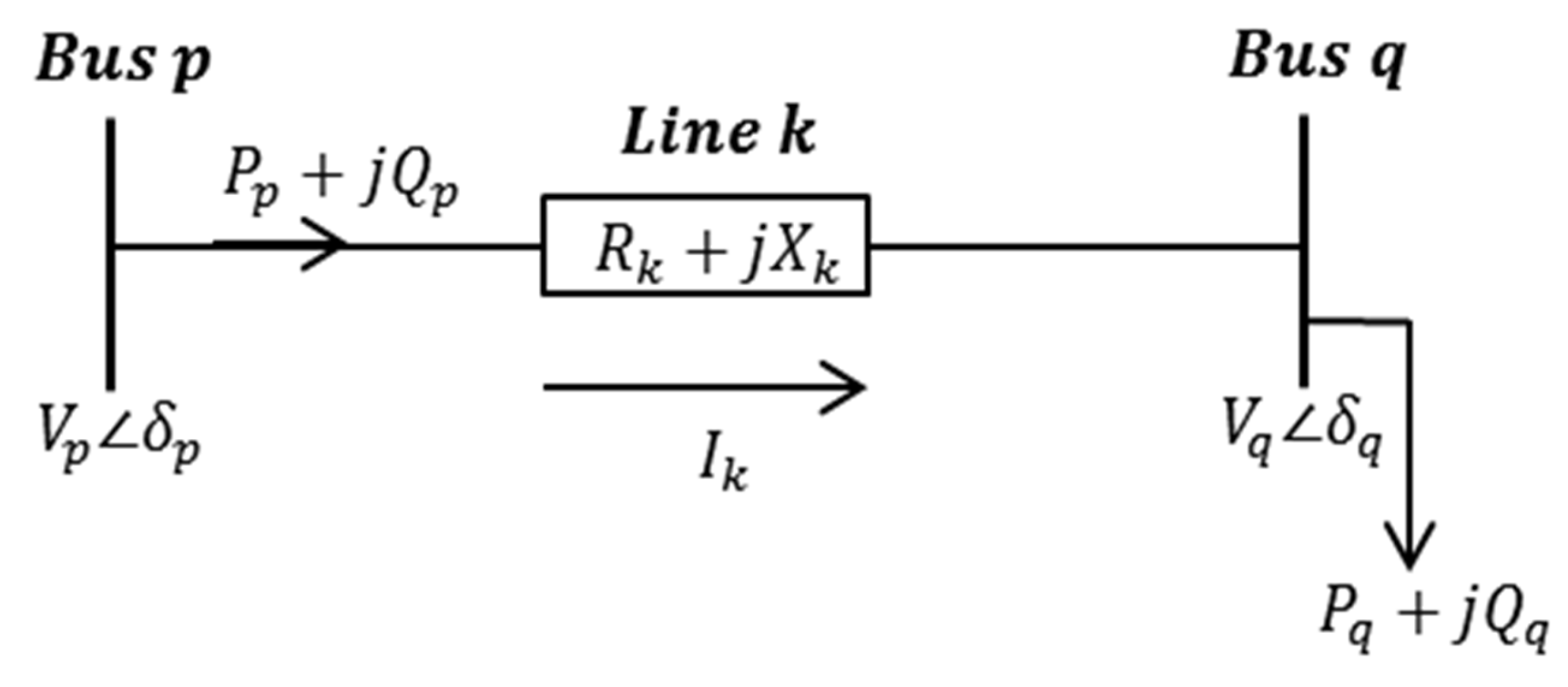
This work presents a voltage stability index (VSI) for steady-state situations, with the goal of discovering nodes with increased susceptibility to voltage collapse. The index, abbreviated as VSI and stated by Equation (12) [31], is derived from power flow analysis and is used to measure voltage stability at each node. For an RDN to function properly, the VSI should be larger than zero. Nodes with lower VSI values require more compensation measures to ensure voltage stability. For Figure 1, the VSI can be calculated at bus q from Equation (12).
V S I = V p 4 4 ( Q P X k + P P R k ) V p 2 + 4 Q P X k + P P R k 2
where Vp is the bus voltage, Rk and Xk are line resistance and reactance, and PP and QP represent effective active and reactive power, respectively.

3. Proposed Impedance-Based Heuristic Approach

This section presents the proposed methodology for the optimal allocation of electric vehicle charging stations (EVCSs) and distributed generators (DGs) in radial distribution networks (RDNs). The approach combines an impedance matrix-based load flow analysis with a deterministic heuristic optimization procedure. The methodology is designed to reduce power losses, reduce voltage deviations, and enhance the voltage stability index, while ensuring economic feasibility under varying electric vehicle hosting factors (EV-HFs).

3.1. Impedance Matrix-Based Load Flow Analysis

The RDN under study consists of a set of buses and radial distribution sections. Bus 1 is considered the slack bus, representing the main power source. The bus impedance matrix (Zbus) is derived from the distribution section-to-bus (DSB) incidence matrix. Generally, the bus voltage for any power network may be found from Equation (13).
[ V b u s ] = [ Z b u s ] [ I b u s ]
where [ V b u s ] and [ I b u s ] are column matrices of N bus and Z b u s is the square matrix (N × N). But in the radial distribution network, the slack bus voltage is known. So, in this case,
[ V b u s ] = V 1 + [ Z b u s ] [ I b u s ]
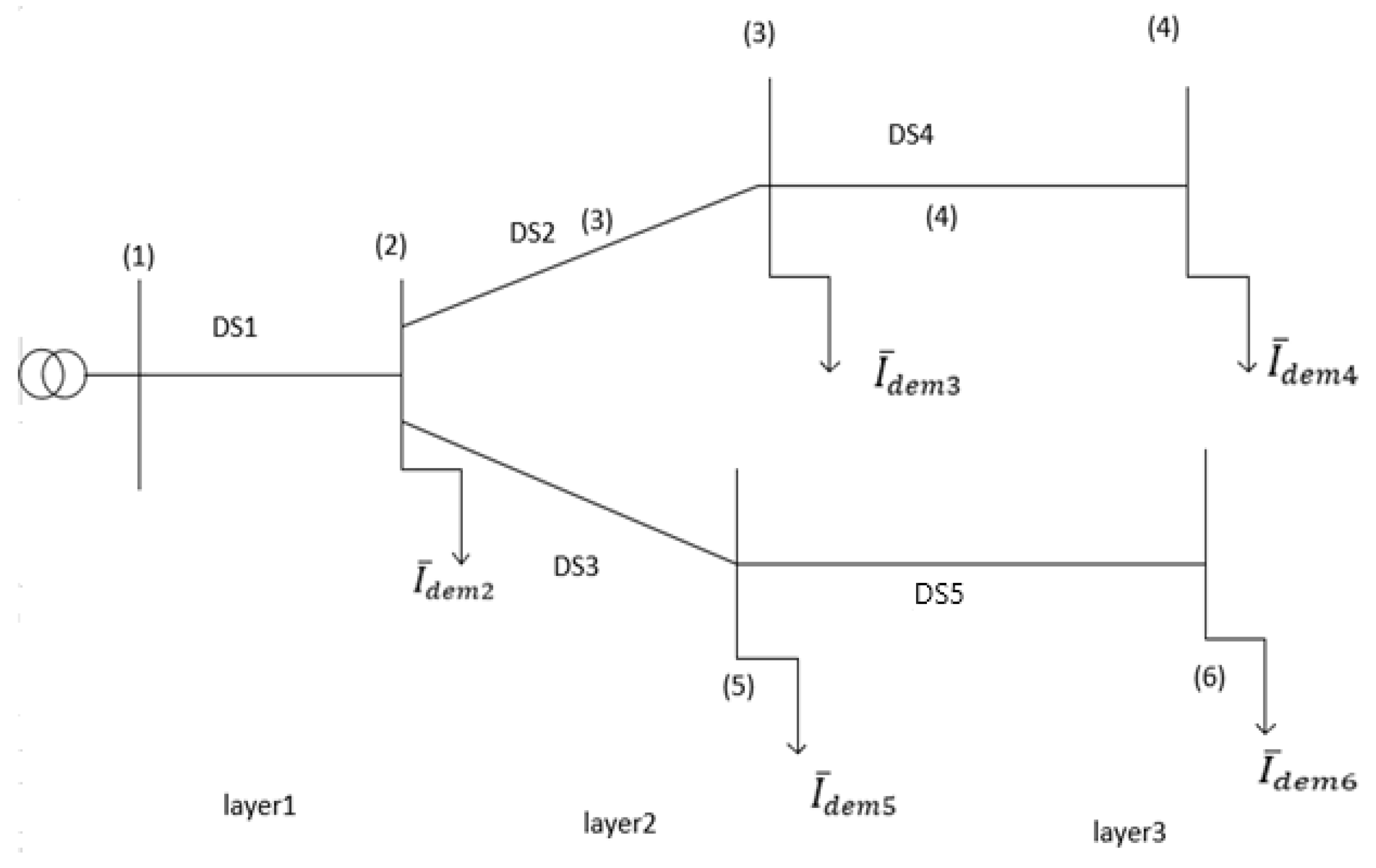
where [ V b u s ] and [ I b u s ] are column matrices of (N − 1) buses starting from bus 2 to bus N and [ Z b u s ] is the (N − 1) × (N − 1) matrix, which refers to the slack bus bar. Construction of the bus impedance matrix using the (DSB) matrix, which is (N − 1) × (N − 1) distribution section-to-bus-incidence matrix. This matrix can be obtained for any radial distribution network using the steps for the simplified network shown in Figure 2.
This distribution network has five DSs and six buses, and the method for constructing the DSB matrix is as follows.
  • Step (1): Initialize the DSB matrix; DSB = zeros (5,5):
DSB = b u s 2 3 4 5 6 D S 1 D S 2 D S 3 D S 4 D S 5 0 0 0 0 0 0 0 0 0 0 0 0 0 0 0 0 0 0 0 0 0 0 0 0 0
  • Step (2): for any distribution section (i), DSB(i, B) = 1 for section (i) supplying the load at bus B:
DSB = b u s 2 3 4 5 6 D S 1 D S 2 D S 3 D S 4 D S 5 1 1 1 1 1 0 1 1 0 0 0 0 0 1 1 0 0 1 0 0 0 0 0 0 1
The bus impedance matrix of the distribution network is obtainable using the DSB matrix in the following equation:
[ Z ¯ b u s ] = [ D S B ] T [ Z ¯ s ] [ D S B ]
where [ Z b u s ] is the bus impedance matrix referring to the slack bus bar and [ Z s ] is a diagonal matrix containing the impedance of ordered distribution sections, so
[ Z s ] = b u s D S 1 D S 2 D S 3 D S 4 D S 5 D S 1 D S 2 D S 3 D S 4 D S 5 Z ¯ s 1 0 0 0 0 0 Z ¯ s 2 0 0 0 0 0 Z ¯ s 3 0 0 0 0 0 Z ¯ s 4 0 0 0 0 0 Z ¯ s 5
  Z b u s = b u s 2 3 4 5 6 2 3 4 5 6 Z ¯ s 1 Z ¯ s 1 Z ¯ s 1 Z ¯ s 1 Z ¯ s 1 Z ¯ s 1 Z ¯ s 1 + Z ¯ s 2 Z ¯ s 1 + Z ¯ s 2 Z ¯ s 1 Z ¯ s 1 Z ¯ s 1 Z ¯ s 1 + Z ¯ s 2 Z ¯ s 1 + Z ¯ s 2 + Z ¯ s 4 Z ¯ s 1 Z ¯ s 1 Z ¯ s 1 Z ¯ s 1 Z ¯ s 1 Z ¯ s 1 + Z ¯ s 3 Z ¯ s 1 + Z ¯ s 3 Z ¯ s 1 Z ¯ s 1 Z ¯ s 1 Z ¯ s 1 + Z ¯ s 3 Z ¯ s 1 + Z ¯ s 3 + Z ¯ s 5
The mentioned detailed formula for calculating the bus impedance matrix is used to derive it, using the new DSB incidence matrix by directly applying Equation (17). Then the bus impedance matrix is obtained, and this matrix is constant during all operations, so it is constructed for the first iteration and used for the whole solution.
The load flow analysis using the bus impedance matrix is as follows:
But   [ I b u s ] = [ I ¯ d e m ]
Then   [ V ¯ b u s ] = [ V ¯ 1 ] [ Z ¯ b u s ] [ I ¯ d e m ]
[ V ¯ b u s ]=   V ¯ 2 V ¯ N , [ V ¯ 1 ] = V ¯ 1 V ¯ 1 V ¯ 1 (N − 1) column matrix
I ¯ d e m =   I ¯ d e m 2 I ¯ d e m 3 I ¯ d e m N   (N − 1) column matrix
  • Assume initially that all bus voltages start from bus number 2 to bus number N is equal to the slack bus voltage.
V ¯ i ( 0 ) = V ¯ 1 ,   k = 0   ( initialize the iteration counter )
2.
Determine the demand load current at each bus.
I ¯ d e m i ( k ) = S ¯ d e m * V ¯ i k i = 2 : N
3.
Then the new bus voltage can be calculated from Equation (24).
[ V b u s ] k + 1 = V 1 [ Z b u s ] [ I d e m ] K
4.
The voltage difference for this iteration is obtained from the Equation (25).
Δ V b u s K + 1 = V b u s K + 1 V b u s K
5.
Compare the maximum voltage difference with an acceptable error (e = 0.00001 pu); if it is less than or equal to this acceptable error, then the final run of the load flow study is obtained. Otherwise, K = K + 1 and return to step 2.
6.
Then the distribution section currents can be obtained using the DSB matrix as follows:
[ I D S ] = [ DSB ] [ I d e m ]
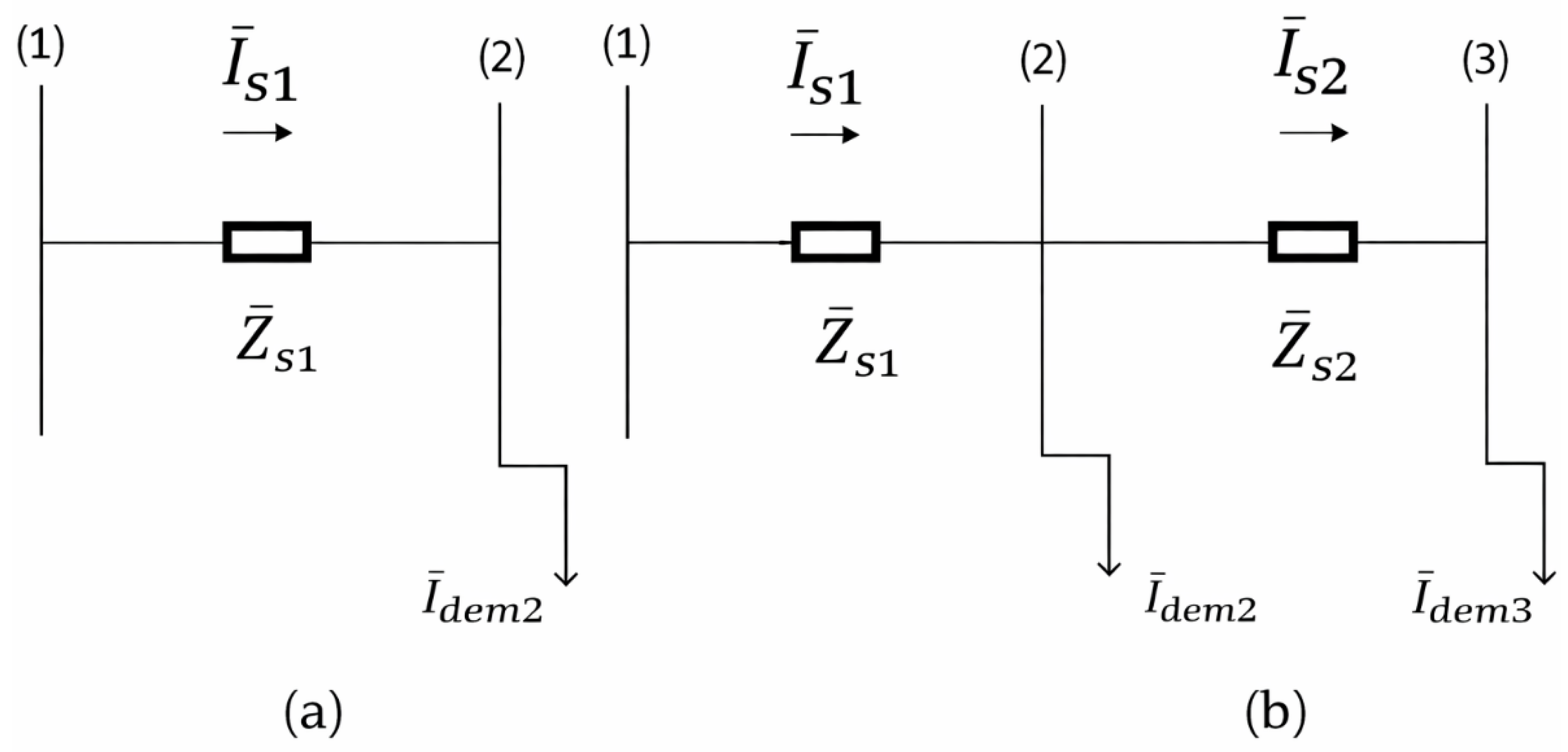
The active and reactive power losses in Figure 3a are calculated as follows:
P l o s s = I s 1 2 R s 1 and   Q l o s s = I s 1 2 X s 1
S l o s s = P l o s s + j Q l o s s
where Z ¯ s 1 = R s 1 + j X s 1
I ¯ s 1 = I ¯ d e m 2
S l o s s = I d e m 2 2 Z ¯ s 1
Z b u s = Z s 1
S ¯ l o s s = [ I d e m   ] * T   Z b u s [   I d e m ]
Also the total active and reactive power losses in Figure 3b can be computed by Equations (33) and (34), respectively.
P l o s s = I s 1 2 R s 1 + I s 2 2 R s 2
Q l o s s = I s 1 2 X s 1 + I s 2 2 X s 2
S l o s s = I s 1 2 Z ¯ s 1 + I s 2 2 Z ¯ s 2
where Z ¯ s 2 = R s 2 + j X s 2
I ¯ s 2 = I ¯ d e m 3 ,   I ¯ s 1 = I ¯ d e m 2 + I ¯ d e m 3
where I ¯ d e m 2 = I d e m 2 θ 2 , I ¯ d e m 3 = I d e m 3 θ 3 , and θ 23 = θ 2 θ 3
So I s 2 2 = I d e m 3 2 , I s 1 2 = I d e m 2 2 + I d e m 3 2 + 2 I d e m 2 I d e m 3 c o s ( θ 23 )
S l o s s = I d e m 2 2 Z ¯ s 1 + I d e m 2 2 Z ¯ s 1 + Z ¯ s 2 + 2 I l 2 I l 3 Z ¯ s 1 cos θ 23
Also the following relation applies:
I ¯ d e m 2 * I ¯ d e m 3 *   Z ¯ s 1 Z ¯ s 1 Z ¯ s 1 Z ¯ s 1 + Z ¯ s 2         I ¯ d e m 2           I ¯ d e m 3
= Z ¯ s 1 I ¯ d e m 2 * Z ¯ s 1 I ¯ d e m 2 * Z ¯ s 1 I ¯ d e m 3 * ( Z ¯ s 1 + Z ¯ s 2 ) I ¯ d e m 3 *   I ¯ d e m 2 I ¯ d e m 3
= Z ¯ s 1   I ¯ d e m 2   I ¯ d e m 2 * + I ¯ d e m 3 * + Z ¯ s 1 I ¯ d e m 3 I ¯ d e m 2 * + I ¯ d e m 3 * + Z ¯ s 2 I d e m 3 2
= Z ¯ s 1 I d e m 2 2 + Z s 1 I l 3 A * I ¯ d e m 2 + Z ¯ s 1 I d e m 3 2 + Z ¯ s 1 I d e m 2 * I ¯ d e m 3 + Z ¯ s 2 I d e m 3 2
= Z ¯ s 1 I d e m 2 2 + Z ¯ s 1 + Z ¯ s 2 I d e m 3 2 + Z ¯ s 1 ( I ¯ d e m 2 * I ¯ d e m 3 + I ¯ d e m 2 I ¯ d e m 3 * )
= Z ¯ s 1 I d e m 2 2 + Z ¯ s 1 + Z ¯ s 2 I d e m 3 2 + 2 I d e m 2 2 I d e m 3 2 Z ¯ s 1 cos ( θ 23 )
Then S ¯ l o s s can be calculated for any RDN by Equation (42):
S ¯ l o s s = [ I d e m   ] * T   Z b u s [   I d e m ]
Also, here the detailed equations derive a new formula used for calculating electrical distribution network losses by applying Equation (42) instead of calculating them using the summation of each individual electrical loss in each distribution branch. So, by using Equation (42) above, the execution time for calculating the power losses can be reduced and the objectives can be calculated quickly, and the proposed method presents very accurate calculations with respect to radial distribution networks.
The novelty of Zbus claimed in the manuscript is the direct method for the construction of it using the proposed DSB incidence matrix, i.e., the application of the DSB matrix to find all branch currents directly. The mentioned detailed equations that are used for calculating the bus impedance matrix are written to derive how Zbus can be calculated using the new DSB incidence matrix by directly applying Equation (17), and the proposed derivation is used to obtain the electrical power losses using the Zbus matrix, i.e., using one equation instead of calculating them using the summation of individual branch losses. So, the power flow solution using Zbus is faster than other published methods.
The advantages of using the bus matrix method as a load flow solution method are the simplicity of constructing it using the DSB incidence matrix and also using the DSB matrix to calculate the distribution branch currents, and the electrical power losses are also determined very easily by one equation without any summations, so the execution time for applying the proposed technique is reduced compared with the exciting methods.

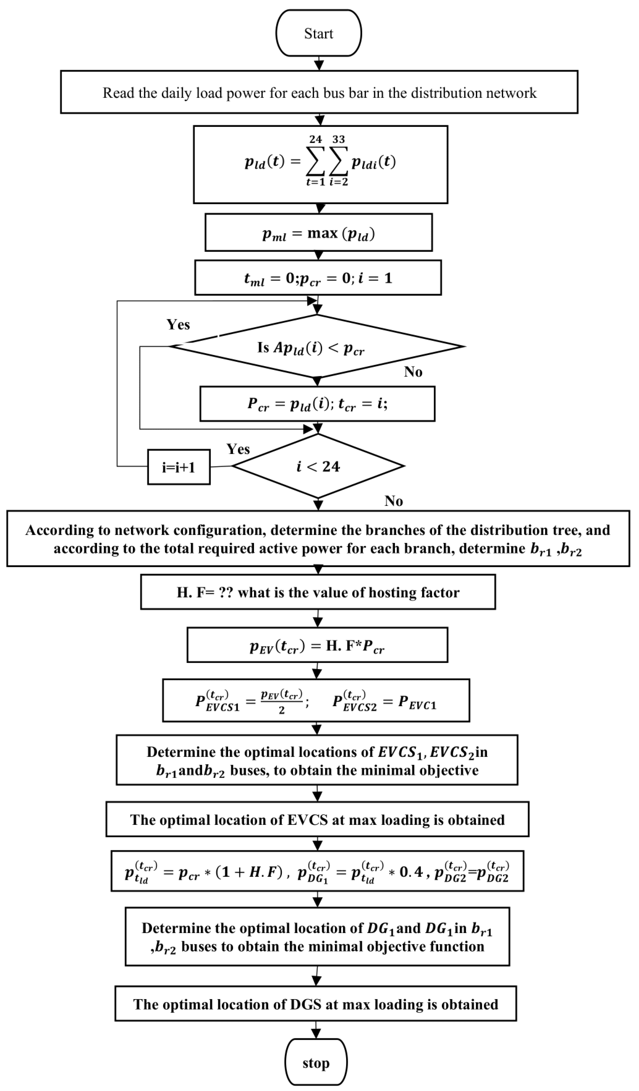
3.2. Heuristic Optimization Procedure at Maximum Loading Condition

The optimization problem is formulated to identify the ideal placement and sizing of EVCSs and DGs under the maximum network loading condition. The stepwise heuristic procedure is as follows:
7.
Identify the Maximum Loading Hour: From the daily load profile, determine the hour with the highest demand.
8.
Initial Placement of EVCSs:
Compute EVCS demand using hosting factors.
Assume two EVCSs with equal demand.
Place them on the first bus of the two most heavily loaded branches.
Run the load flow and compute the objective function Ft.
Search within these branches for placements that minimize Ft.
9.
Sizing of EVCSs:
Incrementally increase the size of one EVCS by ΔP and decrease the other by the same amount.
Recalculate Ft.
If improved, repeat until no further reduction in Ft is obtained.
10.
Placement and Sizing of DGs:
Locate DGs at the same buses as EVCSs.
Initialize their output as 35% of total demand (network load and EVCS demand).
Incrementally adjust DG sizes by ΔP.
Recalculate the total objective function Ft and update until the minimum is reached for each DG.
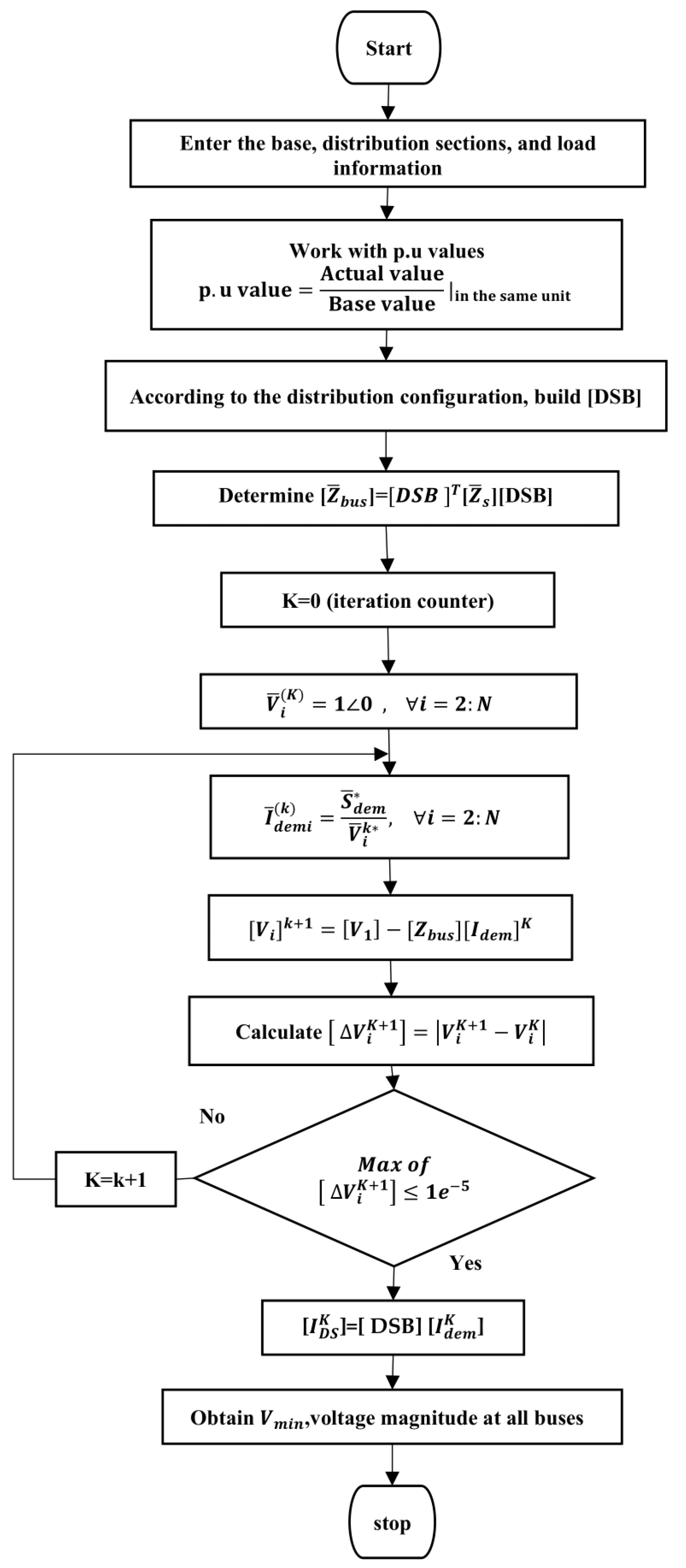
Steps for load flow applying the bus impedance matrix method, and as shown in Figure 4:
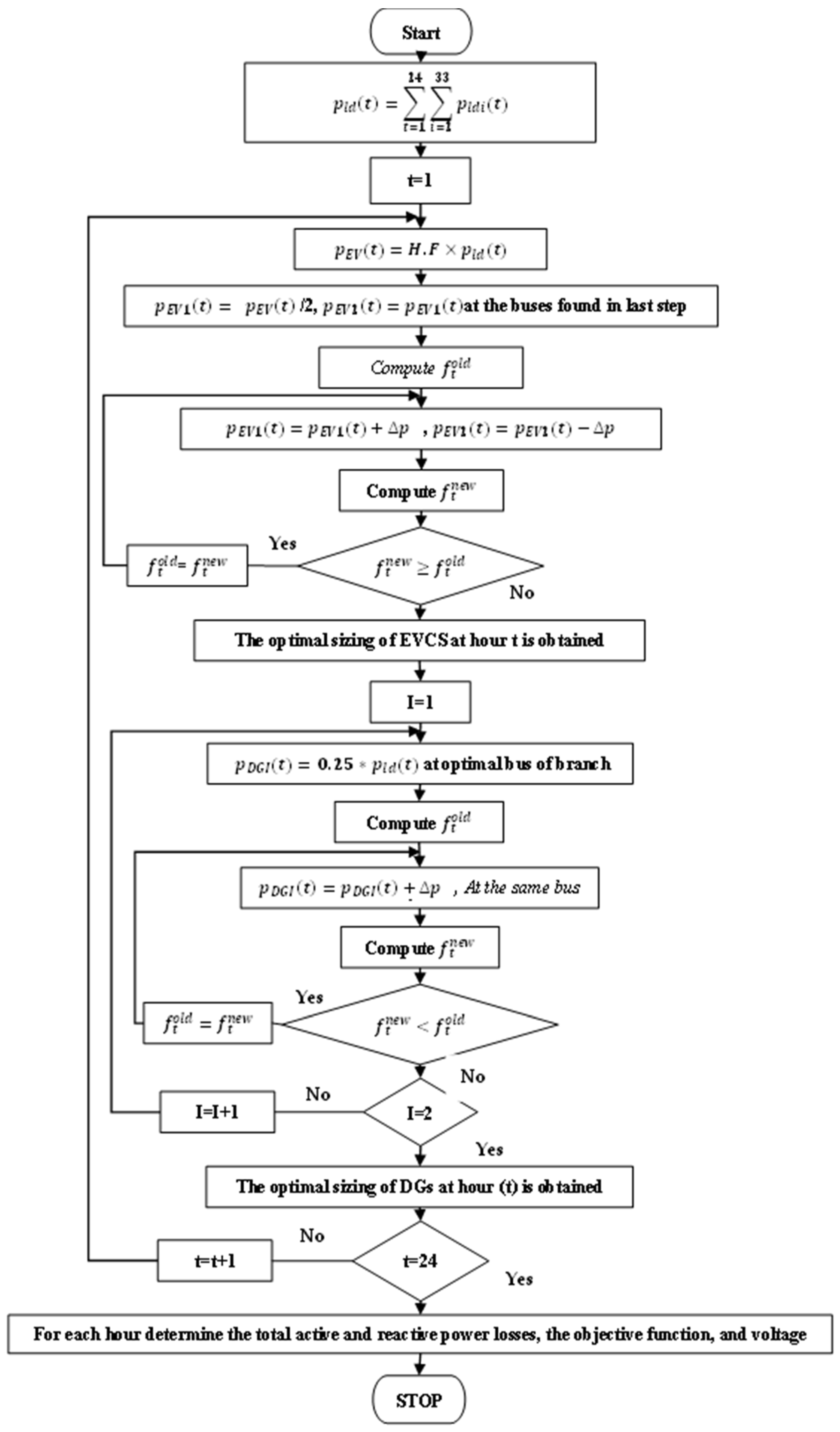
The presented optimization approach is compared with published methods for the 33-bus and 69-bus distribution networks. The comparison derives that the proposed approach is suitable for any distribution network and it is an effective approach compared to other methods. Knowing that the DGs are used to support the distribution network by supplying active power, it is assumed that they supply 35% of the total demand; this value is justified using sensitivity analysis on many loading conditions and is also applied on two electrical distribution networks. ΔP is assumed to be 1.0% of the total active power demand, and the convergence of the proposed approach depends on the value of total overall objective function. When transitioning from the current state condition of the network to another new state, if this objective function is minimized with the new allocation, then this operation is optimal compared to its previous one, but if the overall objective function is increased with the new allocation, then its previous operation is optimal and the process is stopped. This stopping criterion is illustrated in the flowcharts shown in Figure 5 and Figure 6.
At the end of this process, the optimal placement and sizing of both EVCSs and DGs under maximum loading conditions are obtained. Figure 5 and Figure 6 illustrates the flowchart of the optimization methodology at maximum loading.

3.3. Optimization Under Daily Loading Conditions

To extend the optimization beyond the maximum loading hour, the following steps are applied for each hour of the day:
  • Perform load flow for the base case at every hour.
  • Identify the maximum loading hour (hmax) and determine optimal EVCS and DG placement and sizing.
  • Fix the locations of EVCSs and DGs obtained at hmax.
  • For each hour h = 1, …, 24:
  • Calculate EVCS demand using EV-HFs.
  • Apply the heuristic procedure to optimize the sizing of EVCSs and DGs.
  • If h = hmax, skip recalculation of placement.
5.
Repeat until h = 24, at which point the final daily optimal solution is obtained.
This approach ensures that the optimized locations from maximum loading are preserved, while sizing dynamically adapts to hourly variations in load and EV-HF. Figure 6 presents the flowchart of the daily optimization process.
The proposed impedance-based heuristic approach integrates a computationally efficient Zbus-based load flow with an iterative placement–sizing strategy for EVCSs and DGs. Unlike metaheuristic algorithms, this deterministic method achieves fast convergence with minimal computational effort, while ensuring improved network performance across different EV hosting factors and load conditions.

4. Simulation Results

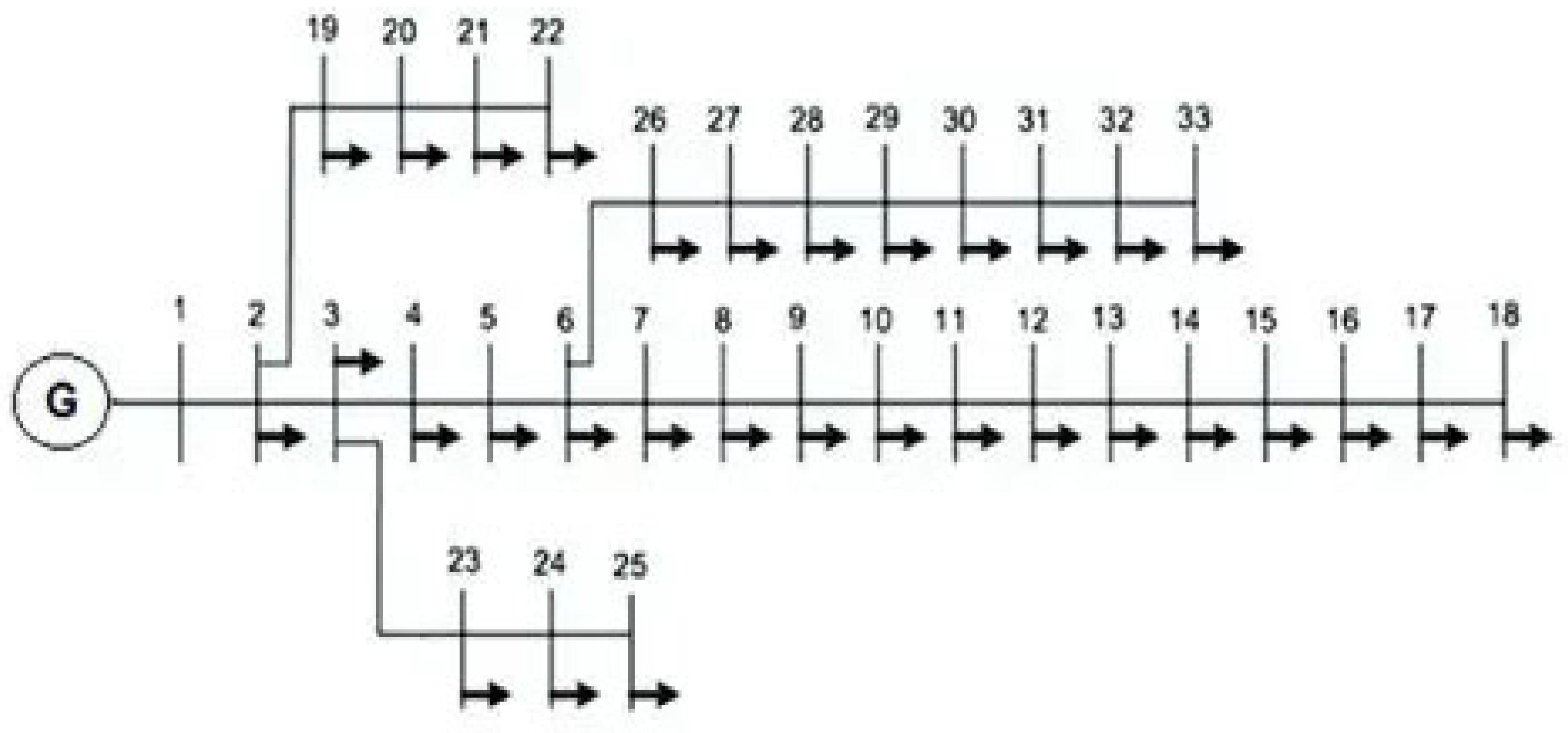
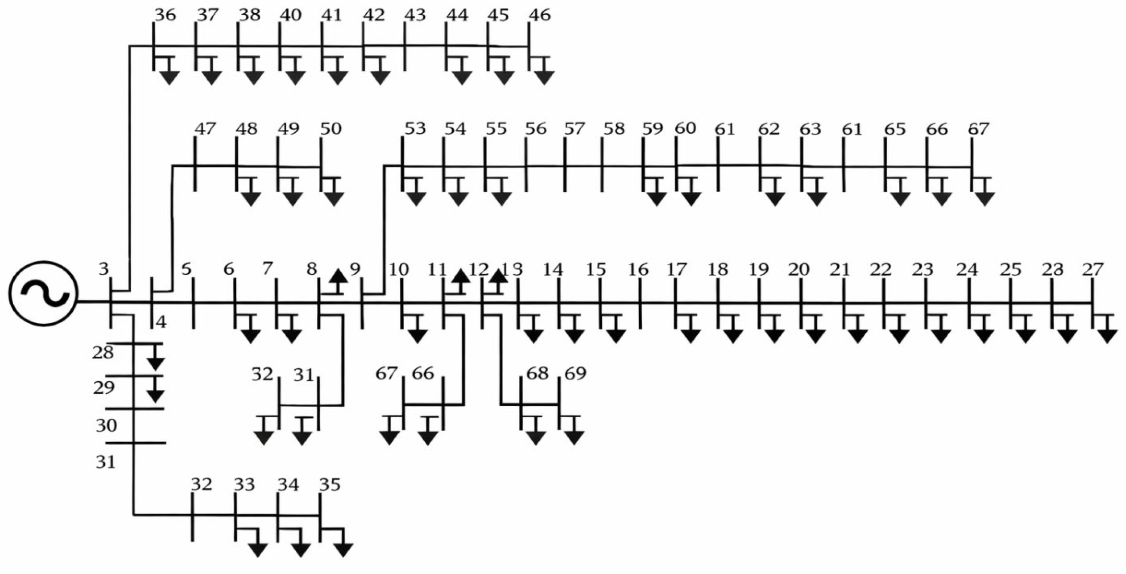
The proposed impedance-based heuristic approach was implemented and verified on two distribution networks, which are the IEEE 33-bus and IEEE 69-bus radial distribution networks [32,33], which are shown in Figure 7 and Figure 8, respectively. The system was analyzed under different loading conditions and EV hosting factors (EV-HFs) to evaluate the effectiveness of coordinated EVCS and DG planning. Performance was evaluated in terms of active power loss reduction and voltage profile improvement, voltage stability index (VSI) improvement, and economic benefits.

4.1. 33-Bus Base Case Analysis

In the base case, the network was simulated without EVCSs or DGs. Table 1 shows the results of the daily hours for the base case study without EVCSs and DGs; these results include the total demand load power, the total active and reactive power losses, and the value of minimum voltage.
The results indicate high active power losses and significant voltage drops, with the minimum bus voltage falling below the acceptable limit of 0.95 pu during peak hours. The maximum loading on the RDN occurs at hour (18), which has active and reactive power losses of 175.7117 kW and 119.0758 kVAR, respectively, while the minimum voltage is 0.9148 pu. These results highlight the need for corrective measures to accommodate future EV penetration while maintaining system reliability.

4.1.1. Coordinated Integration of EVCSs and DGs

Introducing DGs alongside EVCSs provided substantial improvements in both technical and economic performance. The results for connecting EVCSs and DGs with a 40% hosting factor for EVCSs are illustrated in Table 2, which includes the daily hour values of optimal EVCS and DG placement and sizing. The RDN performance under this condition is shown in Table 3, which includes the active and reactive power losses, and the minimum voltage on the distribution network; the percentages of improvement in performance are compared with the base case study. Similarly, Table 4 and Table 5 display the related results at 60% hosting factor for EVCSs with optimal placement and sizing for both EVCSs and DGs.
At 40% EV-HF: Active power losses were reduced by approximately 57% compared with the base case. The minimum bus voltage improved from 0.9148 pu to 0.9654 pu. The VSI values increased, indicating enhanced network stability.
At 60% EV-HF: Losses were similarly reduced, though slightly less effective due to higher load demand. The minimum bus voltage improved to 0.9641 pu, remaining within acceptable operational limits. VSI improvements were sustained, demonstrating the robustness of the method under higher penetration.
These results confirm that the proposed methodology ensures reliable network performance even under heavy EV adoption.
Table 6 presents the comparison between results obtained for the base case, the operation with a 40% EV-HF, and the operation with a 60% EV-HF with respect to the annual energy losses, VSI, VDI, Vmin, the total cost of DGs, the cost of saving energy, and the profit for the system assuming a lifetime of 25 years.

4.1.2. Voltage Profile Improvement

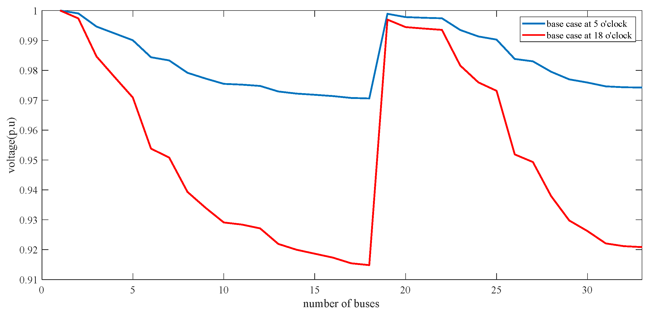
The optimized EVCS and DG allocation significantly enhanced the overall voltage profile of the IEEE 33-bus system. Voltage levels across all buses remained within the acceptable 0.95–1.05 pu band, eliminating the undervoltage problems observed in the base case and EV-only cases. The most pronounced improvements were observed at the weakest buses, where voltage recovery was nearly 5% compared with the base case. The following curve, shown in Figure 9, presents the voltage profile of both the light and maximum loading conditions for the base case study, which shows that the minimum voltage at maximum loading is 0.913 pu.
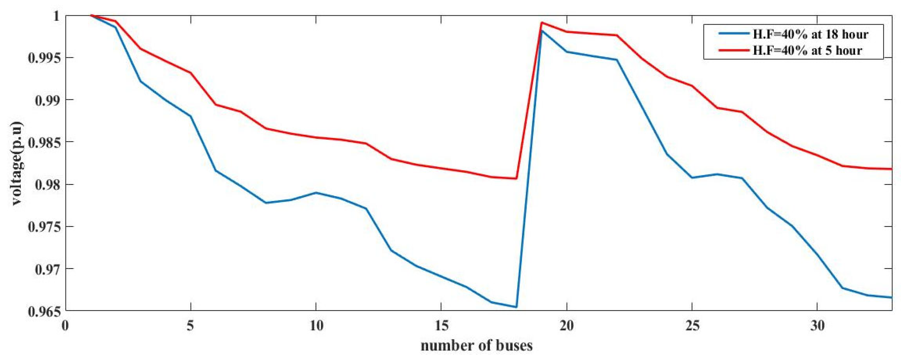
Figure 10 depicts the voltage on the network for the light and maximum loading conditions with an EVCS hosting factor of 40%; here, the minimum voltage is 0.9654 pu.
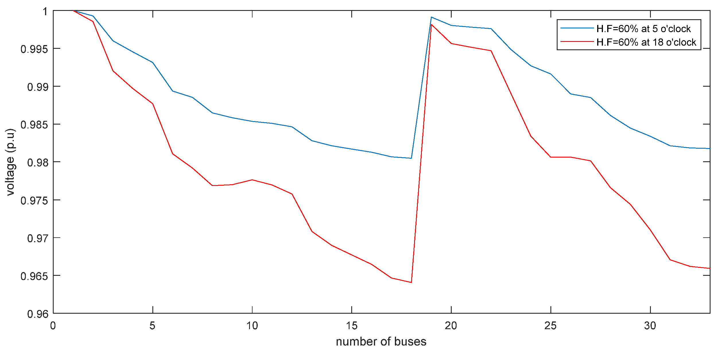
Figure 11 provides the voltage profile for the loading conditions at both hours 5 and 18 with an EVCS hosting factor of 60%: the minimum voltage is 0.9641 pu.
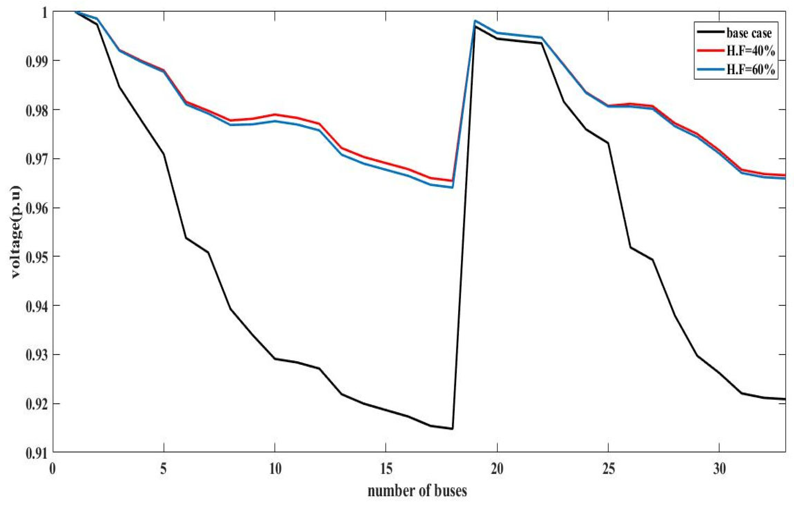
Figure 12 presents the voltage profile comparison at maximum loading condition for the base case, EVCS hosting factor of 40% operating condition, and EVCS hosting factor of 60% operating condition. Although the loading on the network is increased by 40% and 60%, respectively, the minimum voltage is increased to acceptable values compared to that occurring for base case operation.
Table 7 presents the comparisons between published methods and the proposed approach for the 33-bus IEEE distribution network at the heavy loading condition operated at hour 18. The results show that the proposed approach is more effective than the published methods for the same operating condition.

4.2. 69-Bus Distribution Network Results

The application of the proposed approach on the IEEE 69-bus distribution network is presented with comparisons with some published methods at the same operating condition in Table 8.

5. Conclusions

This research described an impedance-based heuristic technique for the optimum placement and size of electric vehicle charging stations (EVCSs) and distributed generators (DGs) in radial distribution networks with different electric vehicle hosting factors (EV-HFs). The proposed impedance matrix-based load flow and analytical loss formulation provided accurate and computationally efficient evaluation of network performance, enabling fast optimization across multiple operating conditions. Simulation results on the IEEE 33-bus system demonstrated that unmanaged EVCS integration leads to higher active power losses and voltage deviations, with minimum bus voltages dropping below acceptable limits. Coordinated EVCS and DG planning significantly improved network performance. At 40% and 60% EV-HFs, active power losses were reduced by nearly 57%, while the minimum bus voltage improved from 0.9148 pu (base case) to 0.9654 pu and 0.9641 pu, respectively. The voltage stability index (VSI) also increased, confirming improved system resilience. Economic analysis indicated strong financial feasibility. The integration of PV-based DGs provided annual cost savings of up to USD 473,550, with a payback period of 7–8 years and substantial long-term profit over the system’s lifetime. The methodology is practical for distribution network operators, as it combines technical benefits (loss minimization and voltage stability) with economic gains, while maintaining computational simplicity compared to population-based metaheuristics. The results of proposed approach for both the 33-bus and 69-bus IEEE electrical distribution networks are compared with the published methods, which demonstrates the effectiveness of the proposed approach.
Future work will concentrate on broadening the suggested framework to include uncertainties in EV demand and in renewable generation. The impact of variable operation costs such as maintenance costs for photovoltaic units and time-of-use electricity pricing should also be taken in calculation for economic calculation and payback time. Also, dynamic voltage stability analysis in high-penetration EV fast-charging scenarios and the incorporation of energy storage technologies to improve flexibility and resilience should be studied.

Author Contributions

Conceptualization, A.A. and A.S.; methodology, A.A.A.E.-E.; software, A.S.; validation, A.A., A.S. and N.E.; formal analysis, N.E.; resources, A.A.A.E.-E.; data curation, A.A., T.A. writing—original draft preparation, A.F.; writing—review and editing, N.E., A.F., I.H., A.A.A.E.-E., T.A.; visualization, A.S.; supervision, I.H.; funding acquisition, A.A. All authors have read and agreed to the published version of the manuscript.

Funding

This research received no external funding.

Institutional Review Board Statement

This study did not involve human participants, animals, or any form of biological material, and therefore, ethical approval was not required. The research conducted is based on engineering simulations and theoretical models. All data used in this study are publicly available or generated through validated computational methods, and no ethical concerns arose in the course of the work.

Data Availability Statement

The data sets used and/or analyzed during the current study are available from the corresponding author on reasonable request.

Acknowledgments

The authors would like to the Electrical Power and Machines Department, Helwan University, Cairo, Egypt, for technical support. The authors declare that the manuscript is an original work and has not been published previously, nor is it under consideration for publication elsewhere.

Conflicts of Interest

The authors declare no competing interests.

Abbreviations and List of Symbols

EVsElectric vehicles
EVCSsElectric vehicle charging stations
HFsHosting factors
EV-HFEV hosting factor
QGDAQuantum-behaved gaussian mutational dragonfly algorithm
DGsDistributed generators
TLBOTeaching–learning-based optimization
MOPSOMulti-objective particle swarm optimization
DEDifferential evolution
GWOGrey wolf optimizer
CSOChicken swarm optimization
LGEGLazy greedy with effective gain
MINLPMixed integer nonlinear programming
DE-HHOHawks optimization
V m i n Minimum voltage on network buses
RDNRadial distribution network
DSBDistribution branches section-to-bus incidence matrix
[ Z b u s ]Bus impedance matrix referring to slack bus bar
[ Z s ]Diagonal matrix containing the impedance of ordered distribution sections
I ¯ d e m i ( k ) Demand load current at bus (i) in iteration (k)
[ V b u s ] k + 1 DN bus voltages in iteration (k + 1)
[ I D S ]Distribution section currents
ACSELAnnual cost saving of energy loss
N b Number of DN buses
P S Active power generated at the slack bus bar
P d e m a n d , i ( h ) Total active power of the load (i) at hour (h)
P E V C S (h)Total active power of the EVCS at hour (h)
P l o s s Total active power loss
VDIVoltage deviation index
VSIVoltage stability index
PSOParticle Swarm Optimization
ABCArtificial Bee Colony
IWOInvasive Weed Optimization
WOAWhale Optimization Algorithm
SASimulated Annealing

References

  1. Yaghoubi, E.; Yaghoubi, E.; Khamees, A.; Razmi, D.; Lu, T. A systematic review and meta-analysis of machine learning, deep learning, and ensemble learning approaches in predicting EV charging behavior. Eng. Appl. Artif. Intell. 2024, 135, 108789. [Google Scholar] [CrossRef] [Scilit]
  2. Campaña, M.; Inga, E. Optimal deployment of fast-charging stations for electric vehicles considering the sizing of the electrical distribution network and traffic condition. Energy Rep. 2023, 9, 5246–5268. [Google Scholar] [CrossRef] [Scilit]
  3. Rajesh, P.; Shajin, F.H. Optimal allocation of EV charging spots and capacitors in distribution network improving voltage and power loss by Quantum-Behaved and Gaussian Mutational Dragonfly Algorithm (QGDA). Electr. Power Syst. Res. 2014, 32, 47–53. [Google Scholar] [CrossRef] [Scilit]
  4. Liu, L.; Xie, F.; Huang, Z.; Wang, M. Multi-objective coordinated optimal allocation of DG and evcss based on the V2G mode. Processes 2021, 9, 18. [Google Scholar] [CrossRef] [Scilit]
  5. Reddy, M.S.K.; Selvajyothi, K. Optimal placement of electric vehicle charging station for unbalanced radial distribution systems. Energy Sources Part. A Recovery Util. Environ. Eff. 2020, 47, 1731017. [Google Scholar] [CrossRef] [Scilit]
  6. Gampa, S.R.; Jasthi, K.; Goli, P.; Das, D.; Bansal, R.C. Grasshopper optimization algorithm based two stage fuzzy multiobjective approach for optimum sizing and placement of distributed generations, shunt capacitors and electric vehicle charging stations. J. Energy Storage 2020, 27, 101117. [Google Scholar] [CrossRef] [Scilit]
  7. Kathiravan, K.; Rajnarayanan, P.N. Application of AOA algorithm for optimal placement of electric vehicle charging station to minimize line losses. Electr. Power Syst. Res. 2023, 214, 108868. [Google Scholar] [CrossRef] [Scilit]
  8. Bilal, M.; Rizwan, M.; Alsaidan, I.; Almasoudi, F.M. AI-Based Approach for Optimal Placement of EVCS and DG with Reliability Analysis. IEEE Access 2021, 9, 154204–154224. [Google Scholar] [CrossRef] [Scilit]
  9. Chippada, D.; Reddy, M.D. Optimal Planning of Electric Vehicle Charging Station along with multiple distributed generator units. Int. J. Intell. Syst. Appl. 2022, 14, 40–53. [Google Scholar] [CrossRef] [Scilit]
  10. Chen, L.; Xu, C.; Song, H.; Jermsittiparsert, K. Optimal sizing and sitting of EVCS in the distribution system using metaheuristics: A case study. Energy Rep. 2021, 7, 208–217. [Google Scholar] [CrossRef] [Scilit]
  11. Deb, S.; Tammi, K.; Gao, X.Z.; Kalita, K.; Mahanta, P. A hybrid Multi-objective Chicken Swarm optimization and teaching learning based Algorithm for Charging Station Placement Problem. IEEE Access 2020, 8, 92573–92590. [Google Scholar] [CrossRef] [Scilit]
  12. Hadian, E.; Akbari, H.; Farzinfar, M.; Saeed, S. Optimal allocation of electric vehicle charging stations with adopted smart charging/discharging schedule. IEEE Access 2020, 8, 196908–196919. [Google Scholar] [CrossRef] [Scilit]
  13. Jin, Y.; Acquah, M.A.; Seo, M.; Han, S. Optimal siting and sizing of EV Charging Station using Stochastic Power Flow Analysis for Voltage Stability. IEEE Trans. Transp. Electrif. 2023, 10, 777–794. [Google Scholar] [CrossRef] [Scilit]
  14. Vijayalakshmi, V.J.; Arumugam, P.; Christy, A.A.; Brindha, R. Simultaneous allocation of EV charging stations and renewable energy sources: An Elite RERNN-m2MPA approach. Int. J. Energy Res. 2022, 46, 9020–9040. [Google Scholar] [CrossRef] [Scilit]
  15. Deb, S.; Gao, X.Z.; Tammi, K.; Kalita, K.; Mahanta, P. A novel chicken swarm and teaching learning based algorithm for electric vehicle charging station placement problem. Energy 2021, 220, 119645. [Google Scholar] [CrossRef] [Scilit]
  16. Hashemian, S.N.; Latify, M.A.; Yousefi, G.R. PEV Fast-Charging Station Sizing and Placement in Coupled Transportation Distribution Networks Considering Power Line Conditioning Capability. IEEE Trans. Smart Grid. 2020, 11, 4773–4783. [Google Scholar] [CrossRef] [Scilit]
  17. Zhang, Y.; Wang, Y.; Li, F.; Wu, B.; Chiang, Y.Y.; Zhang, X. Efficient Deployment of Electric Vehicle Charging Infrastructure: Simultaneous Optimization of Charging Station Placement and Charging Pile Assignment. IEEE Trans. Intelli. Transp. Syst. 2021, 22, 6654–6659. [Google Scholar] [CrossRef] [Scilit]
  18. Battapothula, G.; Yammani, C.; Maheswarapu, S. Multi-objective simultaneous optimal planning of electrical vehicle fast charging stations and DGs in distribution system. J. Mod. Power Syst. Clean Energy 2019, 7, 923–934. [Google Scholar] [CrossRef] [Scilit]
  19. Pal, A.; Bhattacharya, A.; Chakraborty, A. Placement of Electric Vehicle Charging Station and Solar DG in Distribution System considering Uncertainties. Sci. Iran. 2023, 30, 183–206. [Google Scholar] [CrossRef] [Scilit]
  20. Asna, M.; Shareef, H.; Prasanthi, A. Planning of fast charging stations with consideration of EV user, distribution network and station operation. Energy Rep. 2023, 9, 455–462. [Google Scholar] [CrossRef] [Scilit]
  21. Bitencourt, L.; Abud, T.P.; Dias, B.H.; Borba, B.S.; Maciel, R.S.; Quirós-Tortós, J. Optimal location of EV charging stations in a neighborhood considering a multi-objective approach. Electr. Power Syst. Res. 2021, 199, 107391. [Google Scholar] [CrossRef] [Scilit]
  22. Fotopoulou, M.; Pediaditis, P.; Skopetou, N.; Rakopoulos, D.; Christopoulos, S.; Kartalidis, A. A Review of the Energy Storage Systems of Non-Interconnected European Islands. Sustainability 2024, 16, 1572. [Google Scholar] [CrossRef] [Scilit]
  23. Ahmad, F.; Asharf, I.; Marzband, M.; Khan, I. Placement and Capacity of EV Charging stations by considering uncertainties with Energy Management Strategies. IEEE Trans. Ind. Appl. 2023, 59, 3865. [Google Scholar] [CrossRef] [Scilit]
  24. Abdelaziz, M.A.; Ali, A.A.; Swief, R.A.; Elazab, R. A reliable optimal electric vehicle charging stations allocation. Ain Shams Eng. J. 2024, 15, 102763. [Google Scholar] [CrossRef] [Scilit]
  25. Hemeida, A.M.; Bakry, O.; Alkhalaf, S.; Mikhaylov, A.; Zobaa, A.F.; Senjyu, T.; Mikhailef, S.; Dardeer, M. Impact of loading capability on optimal location of renewable energy systems distribution networks. Ain Shams Eng. J. 2024, 15, 102340. [Google Scholar] [CrossRef] [Scilit]
  26. Jia, C.; Liu, W.; Chau, K.T.; He, H.; Zhou, J.; Niu, S. Passenger-aware reinforcement learning for efficient and robust energy management of fuel cell buses. eTransportation 2026, 27, 100537. [Google Scholar] [CrossRef] [Scilit]
  27. Liang, Z.; Luo, Z.; Zhang, B. An Integrated Inductive-Capacitive Nanocrystalline Core for Compact Inductive Power Transfer Systems. IEEE Trans. Power Electron. 2025, 40, 14351–14355. [Google Scholar] [CrossRef] [Scilit]
  28. Wang, D.; He, X.; Fu, C.; Zhao, Q.; Zhang, Z. Dynamic Wireless Charging System for EVs with Uniform Voltage Output Based on Flux Pipe Supply Rail and H-Type Receiver. IEEE Trans. Emerg. Sel. Top. Power Electron. 2024, 13, 4158–4170. [Google Scholar] [CrossRef] [Scilit]
  29. Ramasamy, V.; Zuboy, J.; O’Shaughnessy, E.; Feldman, D.; Desai, J.; Woodhouse, M.; Basore, P.; Margolis, R.U.S. Solar Photovoltaic System and Energy Storage Cost Benchmarks, with Minimum Sustainable Price Analysis: Q1; National Renewable Energy Laboratory (NREL): Golden, CO, USA, 2022. Available online: www.nrel.gov/publications (accessed on 23 September 2023).
  30. Sharma, P.; Chinnappa Naidu, R. Optimization techniques for grid-connected PV with retired EV batteries in centralized charging station with challenges and future possibilities: A review. Ain Shams Eng. J. 2023, 14, 101985. [Google Scholar] [CrossRef] [Scilit]
  31. Shaheen, A.M.; Ellien, A.R.; El-Ela, A.A.; Ali, E.S. Optimal integration of EV charging infrastructure in sustainable distribution systems via growth optimizer-based Hong point estimate. Energy 2025, 318, 134567. [Google Scholar] [CrossRef] [Scilit]
  32. Aljumah, A.S.; Alqahtani, M.H.; Shaheen, A.M.; Ginidi, A.R. Adaptive operational allocation of D-SVCs in distribution feeders using modified artificial rabbits algorithm. Electr. Power Syst. Res. 2025, 245, 111588. [Google Scholar] [CrossRef] [Scilit]
  33. Aljumah, A.S.; Alqahtani, M.H.; Ginidi, A.R.; Shaheen, A.M. Improved Artificial Hummingbird Algorithm for Optimal Allocation of SVCs in Distribution Networks to Maximize Energy Efficiency. J. Mod. Power Syst. Clean Energy 2025, early access. 1–12. [Google Scholar] [CrossRef] [Scilit]
  34. Zaki, M.A.; Mahmoud, T.; Atia, M.; Osman, E.S.A.E.A. Optimal sizing and sitting of electric vehicle charging station by using 100rchimedes optimization algorithm technique. Int. J. Power Electron. Drive Syst. 2021, 12, 2557–2569. [Google Scholar] [CrossRef] [Scilit]
  35. Prempeh, I.; Awopone, A.K.; Ayambire, P.N.; El-Sehiemy, R.A. Optimal allocation of distributed generation units and fast electric vehicle charging stations for sustainable cities. Green Energy Intell. Transp. 2025, 4, 100281. [Google Scholar] [CrossRef] [Scilit]
  36. Rama Prabha, D.; Jayabarathi, T. Optimal placement and sizing of multiple distributed generating units in distribution networks by invasive weed optimization algorithm. Ain Shams Eng. J. 2016, 7, 683–694. [Google Scholar] [CrossRef] [Scilit]
  37. Prakash, D.B.; Lakshminarayana, C. Multiple DG placements in radial distribution system for multi objectives using Whale Optimization Algorithm. Alex. Eng. J. 2018, 57, 2797–2806. [Google Scholar] [CrossRef] [Scilit]
Figure 1. Two bus distribution networks for calculation of VSI.
Energies 19 00753 g001
Figure 2. Simple distribution network.
Energies 19 00753 g002
Figure 3. (a) Two bus network. (b) Three bus network.
Energies 19 00753 g003
Figure 4. Flowchart for the load flow method.
Energies 19 00753 g004
Figure 5. Flowchart of the optimization methodology at maximum loading.
Energies 19 00753 g005
Figure 6. Flowchart of the daily optimization process.
Energies 19 00753 g006
Figure 7. IEEE 33-bus radial distribution network.
Energies 19 00753 g007
Figure 8. IEEE 69-bus radial distribution network.
Energies 19 00753 g008
Figure 9. Light and maximum loading for base case operation.
Energies 19 00753 g009
Figure 10. Light and maximum loading for operation with EVCS and DG at H.F of 40%.
Energies 19 00753 g010
Figure 11. Light and maximum loading for operation with EVCS and DG at H.F of 60%.
Energies 19 00753 g011
Figure 12. Comparison between the base case operation and the operation with the EVCS and DG at a H.F of 40% and 60% for the maximum loading condition.
Energies 19 00753 g012
Table 1. Results for the base case daily operation.
Hours P l o a d (kW)Losses (kW) (Base Case)Reactive Power Loss (kVAR)Minimum Voltage (Base Case)
(pu)
VDI × 10−3VSI
11297.121.881114.84970.9686140.88
21276.121.469314.56080.969013.70.8817
31239.020.760614.0650.969813.10.8846
41213.120.280213.730.970412.80.8867
51204.020.114213.61440.970612.60.8874
61697.551.143834.75520.955031.30.8317
72210.7107.491973.3810.931963.40.7542
82227.6108.154873.83350.9318640.7539
92866.1148.6872100.80820.9240910.7288
102880.8149.4229101.3140.923691.60.7277
112892.7150.0219101.7260.923392.10.7269
122635.6111.230075.32680.932269.20.7553
132550.4105.828371.69770.934265.80.7616
142931.7152.7907103.58460.922493.90.7240
152982.9156.6376106.16220.921296.40.7202
163034.0160.5628108.79430.920098.90.7165
173148.6167.5942113.59620.9173104.10.7081
183254.8175.7117119.07580.9148109.50.704
193057.8127.862386.74280.923881.20.7282
203073.7122.103182.94680.924577.70.7305
213126.8119.773881.55240.924276.30.7295
222993.2103.192670.47350.928965.30.7445
231618.429.163020.02560.961519.40.8548
241591.128.472019.53010.962118.90.8570
Table 2. Results for 40% hosting factor for EVCS operation.
HoursTotal EVCS Consumed Power
(kW)
DG (Size@Location)
(kW)
EVCS (Size@Location)
(kW)
1518.84957@11; 881.84@30235 @11; 283.84@30
2510.44928@11; 861.44@30233@11; 277.44@30
3495.6894@11; 840.6@30230@11; 265.6@30
4485.24868@11; 830.24@30230@11; 255.24@30
5481.6816@11; 765.6@30221@11; 260.6@30
66791130.64@11; 1248.36@30378@11; 301@30
7884.31673.3@11; 1502@30388.3@11; 496@30
8891.041676.6@11; 1501.44@30389.6@11; 501.44@30
91146.441624@11; 1642.44@30584@11; 562.44@30
101152.31630.5@11; 1649.8@30587.5@11; 564.8@30
111157.041629.44@11; 1647.6@30589.44@11; 567.60@30
121054.241537.43@11; 1606.69@30562.43@11; 491.69@30
131020.161529.5@11; 1580.66@30534.5@11; 485.66@30
141172.681618.2@11; 1644.48@30603.2@11; 569.48@30
151193.161629.3@11; 1663.86@30619.3@11; 573.86@33
161213.61630.82@11; 1675.78@30637.82@11; 575.78@30
171295.441668.86@11; 1706.58@30678.86@11; 616.58@30
181301.921662.3@11; 1708.62@30690.3@11; 611.62@30
191223.121547.36@11; 1581.76@30642.36 @11; 580.76@30
201229.481585.72@11; 1725.76@30715.72 @11; 513.76@30
211250.721591.1@11; 1729.62@30731.1@11; 519.62@30
221197.281549.8@11; 1719.48@30714.8 @11; 482.48@30
23647.361244.76@11; 1022.6@30249.76@11; 397.6@30
24636.441220@11; 1016.44@30251@11; 385.44@30
@ means the busbar number.
Table 3. RDN performance analysis results for a 40% hosting factor for EVCS operation.
HoursPower Losses (kW)% Decrease in Active Power LossesReactive Power Loss (kVAR)% Decrease in Reactive LossesMinimum Voltage
(pu)
% Improvement in VoltageVDI × 10−3VSI
111.43047.87.65548.50.98071.255.20.9326
211.35647.17.59847.80.98081.225.20.9310
311.05746.77.39047.40.98121.185.10.9294
410.91546.27.29046.90.98131.1250.9281
511.338543.67.56544.40.98071.045.50.9251
624.32452.4416.64852.10.97432.028.80.9400
748.59854.833.59554.20.96853.92120.9588
848.89554.833.78754.20.96823.9112.30.9586
964.02856.943.93356.40.96824.78130.9563
1064.28656.944.12156.50.96834.84130.9566
1164.557.144.2556.50.96814.8513.30.9563
1247.94856.932.82556.40.9734.389.90.9538
1345.729756.831.31356.30.97324.179.70.9544
1465.6157.144.96456.60.96764.9140.9550
1567.12757.146.01456.70.96795.0613.80.9550
1668.757.247.0856.70.96795.206140.9544
1771.33857.448.831570.96635.34115.50.9541
1874.54557.550.98757.20.96545.5316.20.9533
1955.12156.937.33956.90.96774.7514.10.9484
2052.20157.235.628570.96964.8711.40.9502
2151.42257.135.066570.96924.86911.70.9497
2244.99256.430.66956.50.97124.5510.20.9490
2314.52750.29.89250.60.97751.666.50.9403
2414.250.19.65550.60.97781.636.30.9400
Table 4. Results for 60% hosting factor for EVCS operation.
HoursTotal EVCS Consumed Power
(kW)
DG (Size@Location)
(kW)
EVCS (Size@ Location)
(kW)
1778.261059.26@11; 1019@30359.26@11; 419@30
2765.661038.9@11; 926.76@30358.9@11; 406.76@30
3743.4999.7@11; 963.7@30359.7@11; 383.7@30
4727.86970.96@11; 946.9@30360.96@11; 366.9@30
5722.4923.4@11; 889@30343.4@11; 379@30
61018.51318.7@11; 1384.8@30588.7@11; 429.8@30
71326.421853.24@11; 1743@30593.24@11; 733@30
81336.561857.96@11; 1738.6@30597.96@11; 738.6@30
91719.661900.66@11; 1912@30892.66@11; 827@30
101728.481902.85@11; 1921.63@30896.85@11; 831.63@30
111735.621910.62@11; 1915@30900.62@11; 835@30
121581.361790.76@11; 1840.6@30851.76@11; 729.6@30
131530.241770.24@11; 1810@30811.24@11; 719@30
141759.021900.32@11; 1910.7@30911.32@11; 847.7@30
151789.741930.74@11; 1930@30941.74@11; 848@30
1618201925@11; 1940@30965@11; 855@30
171889.161965.16@11; 1960@301008.16@11; 881@30
181952.881990.88@11; 1986@301056.88@11; 896@30
191834.681860.68@11; 1857@30980.68@11; 854@30
201844.221925.22@11; 1960@301087.22@11; 757@30
211876.081950.2@11; 1968.9@301120.2@11; 755.9@30
221795.921895.92@11; 1945@301079.92@11; 716@30
23971.041364.04@11; 1212@30389.04@11; 582@30
24954.661337.86@11; 1201.8@30387.86@11; 566.8@30
@ means the busbar number.
Table 5. RDN performance analysis results for a 60% hosting factor for EVCS operation.
HoursPower Losses (kW)% Decrease in Active Power LossesReactive Power Loss (kVAR)% Decrease in Reactive Power LossesMinimum Voltage
(pu)
% Improvement in VoltageVDI × 10−3VSI
111.51747.47.71548.190.98051.235.30.9316
211.71945.47.83246.20.98031.175.60.9292
311.18246.27.47646.80.98081.135.20.9283
411.01945.77.36446.40.9811.095.20.9268
511.38943.47.60144.20.98051.025.60.9242
624.452.316.711520.9741.988.90.9390
748.65754.733.64154.20.9693.9812.20.9585
848.97554.733.8454.20.96813.8912.60.9581
964.04756.943.93456.40.96814.7713.50.9549
1064.31456.944.12556.40.96814.8213.60.9548
1164.53356.944.25156.50.96784.8213.90.9549
1247.97856.932.81656.40.97204.2610.50.9519
1345.77956.731.32056.30.97234.0810.40.9526
1465.6825744.96556.60.96704.8314.80.9536
1567.15657.145.99756.70.96745.0214.40.9539
1668.75857.247.05456.70.96705.1215.10.9525
1771.45457.448.85456.90.96515.2116.50.9523
1874.67857.551.02457.10.96415.3817.40.9513
1955.23156.837.39156.90.96694.6614.70.9472
2052.30857.235.656570.96844.7512.30.9485
2151.52156.935.10761.90.96814.7512.40.9483
2245.07256.330.69356.40.97044.4610.70.9479
2314.59349.99.93750.40.97731.646.60.9401
2414.26649.99.70050.30.97761.616.40.9398
Table 6. The impact of EV-HF on the objectives under different operating situations.
Operating ConditionBase Case40% EV-HF60% EV-HF
E l o s s   a n n u a l (kWh)868.729 × 103381.128 × 103381.873 × 103
VSI at max. loading0.7040.95330.9513
VDI at max. loading109.5 × 10−316.2 × 10−317.4 × 10⁻³
V m i n at max loading (pu)0.91480.96540.9641
Costs of used DGs (USD)-3.405 × 1063.976 × 106
Annual saving costs (USD)-468.85 × 103473.55 × 103
Payback period (year)-7.38.4
Total profit for 25-year lifetime (USD).-8.3 × 1067.86 × 106
Table 7. Comparison between published methods and the proposed approach at the heavy loading condition (hour 18) of the IEEE 33-bus distribution network.
MethodOperated withPower Losses (kW)Minimum Voltage
(pu)
Simulation Time (Sec)Total Number of Iterations
PSO [34]EVCSs and DGs77.47380.9562NANA
CS [34]EVCSs and DGs77.24820.9563NANA
AOA [34]EVCSs and DGs77.24750.9579NANA
Proposed ApproachEVCSs and DG74.5450.96542.117
EVCSs only229.58400.88761.8213
DGs only74.2100.96921.8213
Table 8. Comparison between published methods and the proposed approach for the IEEE 69-bus distribution network at the same operating condition.
MethodPower Losses (kW)Minimum Voltage
(pu)
Simulation Time (Sec)Total Number of Iterations
PSO [35]83.20.984NANA
ABC [35]720.987NANA
IWO [36]13.640.99464.5NA
WOA [37]69.720.9780NANA
SA [37]16.26 NANA
Proposed Approach8.20.99382.4522
Disclaimer/Publisher’s Note: The statements, opinions and data contained in all publications are solely those of the individual author(s) and contributor(s) and not of MDPI and/or the editor(s). MDPI and/or the editor(s) disclaim responsibility for any injury to people or property resulting from any ideas, methods, instructions or products referred to in the content.