Article

Less Is More: Data-Driven Day-Ahead Electricity Price Forecasting with Short Training Windows

by
Vasilis Michalakopoulos
*,
Christoforos Menos-Aikateriniadis
,
Elissaios Sarmas
,
Antonis Zakynthinos
,
Pavlos S. Georgilakis
and
Dimitris Askounis
School of Electrical & Computer Engineering, National Technical University of Athens, 15780 Athens, Greece
*
Author to whom correspondence should be addressed.
Energies 2026, 19(2), 376; https://doi.org/10.3390/en19020376
Submission received: 13 December 2025 / Revised: 4 January 2026 / Accepted: 9 January 2026 / Published: 13 January 2026

Abstract

Volatility in the modern world and electricity Day-Ahead Markets (DAMs) usually makes long-term historical data irrelevant or even detrimental for accurate forecasting. This study directly addresses this challenge by proposing a novel forecasting paradigm centered on extremely short training windows, ranging from 7 to 90 days, to maximize responsiveness to recent market dynamics. This volatility-driven approach intentionally creates a data-scarce environment where the suitability of deep learning models is limited. Building on the hypothesis that shallow machine learning models, and more specifically boosting trees, are better adapted to this reality, we evaluate four models, namely LSTM with feed-forward error correction, XGBoost, LightGBM, and CatBoost, across three European energy markets (Greece, Belgium, Ireland) using feature sets derived from ENTSO-E forecast data. Results consistently demonstrate that LightGBM provides superior forecasting accuracy and robustness, particularly when trained on 45–60 day windows, which strike an optimal balance between temporal relevance and learning depth. Furthermore, a stronger capability in detecting seasonal effects and peak price events is exhibited. These findings validate that a short-window training strategy, combined with computationally efficient shallow models, is a highly effective and practical approach for navigating the volatility and data constraints of modern DAM forecasting.

1. Introduction

1.1. Motivation

Accurate day-ahead electricity price forecasting is a strategic necessity in liberalized power markets. Market participants are increasingly exposed to financial risks driven by the rising volatility of electricity wholesale prices, volatility that stems not only from demand fluctuations and generation intermittency but also from evolving regulatory frameworks, bidding rules, and cross-border interconnections [1]. In this environment, the ability to anticipate price spikes, imbalance costs, or low-margin conditions with even marginally improved accuracy can translate directly into competitive advantage or avoided financial loss [2].
The European electricity market landscape has shifted toward real-time responsiveness and market coupling. As trading horizons shrink and operational constraints tighten, forecasting tools must now support continuous adaptation. Traditional models based on extensive historical data, often spanning multiple years, fail to reflect recent structural shifts or evolving participant behavior. In fast-changing regulatory contexts or new market entries (e.g., asset commissioning, portfolio restructuring), historical depth is not a luxury forecasters can rely on.
Price formation in Day-Ahead Markets (DAMs) is now influenced by a combination of complex drivers: dynamic merit order reshuffling due to renewable and gas pricing [3], shifting congestion patterns [4], balancing reserve valuations, and increasingly, by cross-zonal flows managed through EUPHEMIA-based market coupling [5]. Accurate modeling under such conditions requires not just predictive precision but responsiveness to short-term signals. Short training windows offer a pragmatic solution—especially when system behavior is non-stationary or when forecasts must be deployed with minimal delay or localized data only.
Moreover, recent developments in grid flexibility [6,7], prosumer participation [8,9], and decentralized optimization [10,11] require forecasting approaches that are not only accurate in average metrics [12] but also sensitive to extremes—such as peak price spikes or demand troughs [13,14]. These are the events that test the limits of asset profitability and system resilience. In this context, models that learn quickly from short, recent histories and adapt to seasonal dynamics are increasingly valuable. Against this backdrop, our work focuses on a critical but underexplored question: how can machine learning (ML) models be optimized to deliver accurate price forecasts when constrained to short historical datasets? This question is directly relevant to energy traders, Virtual Power Plant (VPP) operators, and Transmission System Operators (TSOs) working in highly dynamic or data-scarce environments [15].
We propose a focused short-window training benchmark study across three European markets (Greece, Ireland, and Belgium) strategically selected to represent a spectrum of European grid characteristics: Greece represents a market with high solar penetration and recent regulatory transformation; Ireland offers a unique island system with high wind dependency; and Belgium serves as a highly interconnected central European hub. Our modeling pipeline (which includes a comprehensive set of forecasting models, such as LightGBM, XGBoost, CatBoost, and an LSTM with feed-forward error correction (FFEC), benchmarked against a naive baseline) relies exclusively on forecasted features, replicating the real information set available to market actors at the time of DAM bidding. This ensures the validity of results for operational use.

1.2. Related Work

DAM price forecasting has been a highly active area of research over the past decade that has increasingly drawn the attention of academic communities, while many state-of-the-art practices have been proposed and implemented, paving the way for accurate and reliable forecasting models. According to the comprehensive review of the methods proposed for market price forecasting spanning 2014 to 2021 by Lago et al. [16], the field is highly diverse, with solutions belonging to three categories, i.e., statistical, ML, and hybrid methods. For the scope of this study, the focus will be on ML-oriented studies published after 2021 to highlight the latest advances in the sector. Additionally, the reviewed studies are further categorized based on the nature of their contribution, distinguishing between those that focus on model-centric innovations, those that emphasize data-centric and scenario-based strategies, and those that utilize both approaches.

1.2.1. Model-Based Approaches

Initially focusing on research that mainly involves novelty surrounding a ML model’s architecture and several methods aimed at optimizing it, Bozlak et al. [17] proposed a hybrid model by merging a Convolutional Neural Network (CNN) with a Long Short-Term Memory (LSTM) model, trained on electricity pricing data from the German electricity market, incorporating total hourly consumption as an exogenous input. The dataset spanned from early 2019 until late 2021, and the proposed model generally outperformed both a simple LSTM and a Seasonal Autoregressive Integrated Moving Average model with exogenous variables (SARIMAX). However, the former provided better results when tested on data from 2020 due to increased noise and volatility. Experimentation with model hybridization was also the focus of Qiang Tan et al. [18], who formed four seasonal datasets, each consisting of five years of historical data from the Australian National Electricity Market, and trained a three-stage hybrid model. The model consisted of an initial time-series decomposition into Intrinsic Mode Functions through improved complete ensemble empirical mode decomposition with adaptive noise, followed by a CNN module for local feature extraction and a stacked sparse denoising autoencoder for robust nonlinear feature learning. The proposed solution proved to be consistently the best-performing model compared to traditional ML and Deep Learning (DL) models, as well as hybrid decomposed and non-decomposed variants. In the same manner, Li et al. [19] used historical hourly data from a regional Chinese market to train a proposed hybrid combination of a Gated Recurrent Unit (GRU) with a Light Gradient Boosting Machine (LightGBM), improved through Bayesian optimization. The training data spanned over a year, and the testing period lasted over 3 months, covering multiple temporal patterns. Their method proved consistently more accurate than its non-optimized variant and a baseline GRU model, improving forecasts by 3.3% and 1.6%, respectively. Similarly, focusing on merging hybrid models with further enhancements, Mubarak et al. [20] trained a combination of a hybrid model consisting of a CNN and a Bidirectional LSTM (BiLSTM) and an auto-regression model, for nonlinear and linear modeling, respectively, on one year of hourly data from the UK and German electricity markets separately, and experimented with different hyperparameter optimization techniques like random search, a genetic algorithm, and particle swarm optimization (PSO). The results showed that PSO achieved a decrease in Root Mean Square Error (RMSE) of 7–9% and Mean Absolute Error (MAE) of 10–19%, compared to the other techniques, including a non-optimized one, in the UK market, while the decrease was around 10–17% with respect to RMSE and 11–24% with respect to MAE in the German market. Also, in a comparable yet distinct approach, Kitsatoglou et al. [21] trained multiple statistical, ML, and DL models on hourly historical pricing, load, and generation data over the span of a year from the German market and experimented with different ensemble strategies to further enhance the robustness and accuracy of day-ahead forecasts. Notably, the methods involved selected the single best-performing model from the previous day and the model with the lowest average hourly MAE over the past 20 days. Additionally, ensemble strategies were tested, such as combining the top models from the last three days using various weighting schemes, as well as taking a simple average of their predictions. Tested only on 28 days of data, the Multilayer Perceptron (MLP) was the best single model, and all custom ensemble models outperformed all individual models except MLP, while the strategy involving the best-performing model per hour consistently had the best overall performance. Overall, these approaches, by leveraging architectural innovations, have demonstrated consistent performance gains over conventional methods.

1.2.2. Data-Centric or Scenario-Based Approaches

Several studies focused on strategies that surround training data and certain scenarios. For example, Yorat et al. [22] focused on the Turkish market and used lagged electricity prices, exchange rates, stock market indices, natural gas prices, and cross-border electricity prices from neighboring countries to construct a comprehensive feature set for training regressors like Multi-linear Regression (MLR) and ARIMA, as well as an Extreme Gradient Boosting (XGBoost) model. The results showed the superiority of the latter, which outperformed both MLR and ARIMA in all evaluation metrics with an R 2 of 95.27%. Likewise, Tschora et al. [15] trained an auto-regressive model and several ML models, like a Support Vector Regressor (SVR), a Random Forest model, a Deep Neural Network (DNN), and a CNN, on historical data from the German, French, and Belgian markets while focusing on several scenarios and data refinements. Specifically, they experimented with two different periods of 5 years, a single-country and multi-country training scenario, and with an enhanced version of the original dataset by adding features like forecasts for demand and generation, stock market indices, and cross-border pricing. The results showed that DNNs and SVRs, trained with the enriched feature set, consistently outperformed traditional models and benchmarks across all markets by achieving up to 15% lower RMSE. In a slightly different approach, Sun et al. [23] used historical pricing, load, generation, and weather data over 15-minute intervals for one year from the Chinese market and trained a gradient-boosting decision tree (GBDT), enhancing it with several algorithms. Specifically, in the first experiment, a segmentation based on load rate was performed by comparing price and system load rate curves, followed by the second experiment, where they also performed parameter optimization for the GBDT. In the third one, the authors added an additional final deviation correction step in peak and flat time periods to calibrate the predictions based on past deviation trends. The results demonstrated a consistent improvement in forecast accuracy across these three experimental schemes, culminating in a Mean Absolute Percentage Error (MAPE) reduction of approximately 50–60% from the first to the third approach. In summary, these studies highlight the critical role of enriched feature sets and carefully designed training scenarios in improving forecast accuracy.

1.2.3. Mixed Approaches

Some researchers sought to integrate both model-centric and data-centric or scenario-based strategies within a unified forecasting framework. Such an example is the study by Micu et al. [24], who trained a hybrid model combining a CNN with BiLSTMs on a dataset consisting of 3 years of data from the United Kingdom market. The input features included historical pricing, demand, generation, weather, and calendar data, while the results showed promising forecast accuracy with MAPE as low as 3.3% for days with generally stable prices; however, the model struggled with high volatility and large price spikes. In a related approach, Pavicevic et al. [25] formed a dataset from hourly historical pricing, weather, and time data spanning over a period of nine years from the Hungarian Day-ahead spot market and used it to train a fully connected neural network (Dense), CNN, LSTM, auto-regressive LSTM, and two hybrid models combining a Dense with an LSTM and a CNN, respectively. Additionally, they experimented with an expanded dataset from 2011 onward and improved it by adding a seasonal difference feature that captures the difference in pricing per hour compared to the same hour one year before. The results indicated a superior performance from the hybrid model containing convolutional layers over both datasets, while it benefits from the expansion, providing more robust forecasts. Lastly, focusing on more complex models and data-driven scenarios, Nitsch et al. [26] utilized the AMIRIS simulator to generate more than 100 total scenarios, each containing a full year of hourly data based on different combinations of flexibility and renewable energy capacity. The authors conducted experiments by separately training an N-Beats model and a Temporal Fusion Transformer (TFT) in multiple training/testing splits by varying the number of scenarios used for training and testing. As a result, the TFT consistently offers improved performance over N-Beats and other naive approaches, mainly due to its ability to utilize future covariates. Additionally, increased flexibility and a higher number of training scenarios led to significantly better performance across all models. Ultimately, by integrating all these different strategies together, mixed approaches aim to achieve an even more robust generalization and adaptability across diverse market conditions.

1.3. Contribution

This study adopts an approach aligned with the second category (Section 1.2.2), since it uses data enhancements and specific training scenarios that benchmark multiple ML models. Compared to the reviewed literature, the variable look-back windows used by the proposed training pipeline and the analysis per calendar month and season are the determining factors that demonstrate the innovative contributions to the field. Specifically, the state-of-the-art practices used in this paper, based on recent literature, as well as the novel advancements proposed, can be summarized as follows:
  • Short-History ML Forecasting: Demonstrates the effectiveness of ML models trained on short historical DAM prices and energy data, addressing the challenge of non-stationary system behavior and the limited relevance of older data in fast-evolving electricity markets.
  • Realistic and Operational Benchmarking: Establishes a practical benchmarking framework across three diverse European markets (Greece, Belgium, Ireland), using only forecasted features available at the time of bidding to simulate real-world decision-making.
  • Evaluation of ML Models with a Focus on Boosting Trees: Includes a diverse set of forecasting models, including LightGBM, CatBoost, XGBoost, LSTM, and a naive baseline. The superior performance of boosting tree models in short-history, high-variability DAM scenarios is demonstrated.
  • Focus on Extreme and Seasonal Events: Emphasizes model sensitivity not only to average performance but also to price extremes (e.g., spikes, troughs), reflecting the real financial and operational risks faced by market participants for each season.

1.4. Structure

The remainder of this paper is organized as follows. Section 2 outlines the methodology of our experiments, including data pre-processing steps, forecasting methods, and a brief overview of European market structures, with a focus on the Greek market. Section 3 presents the benchmark analysis across three market examples. Section 4 provides concluding remarks and discusses future directions.

2. Methodology

2.1. Data Pre-Processing and Preparation

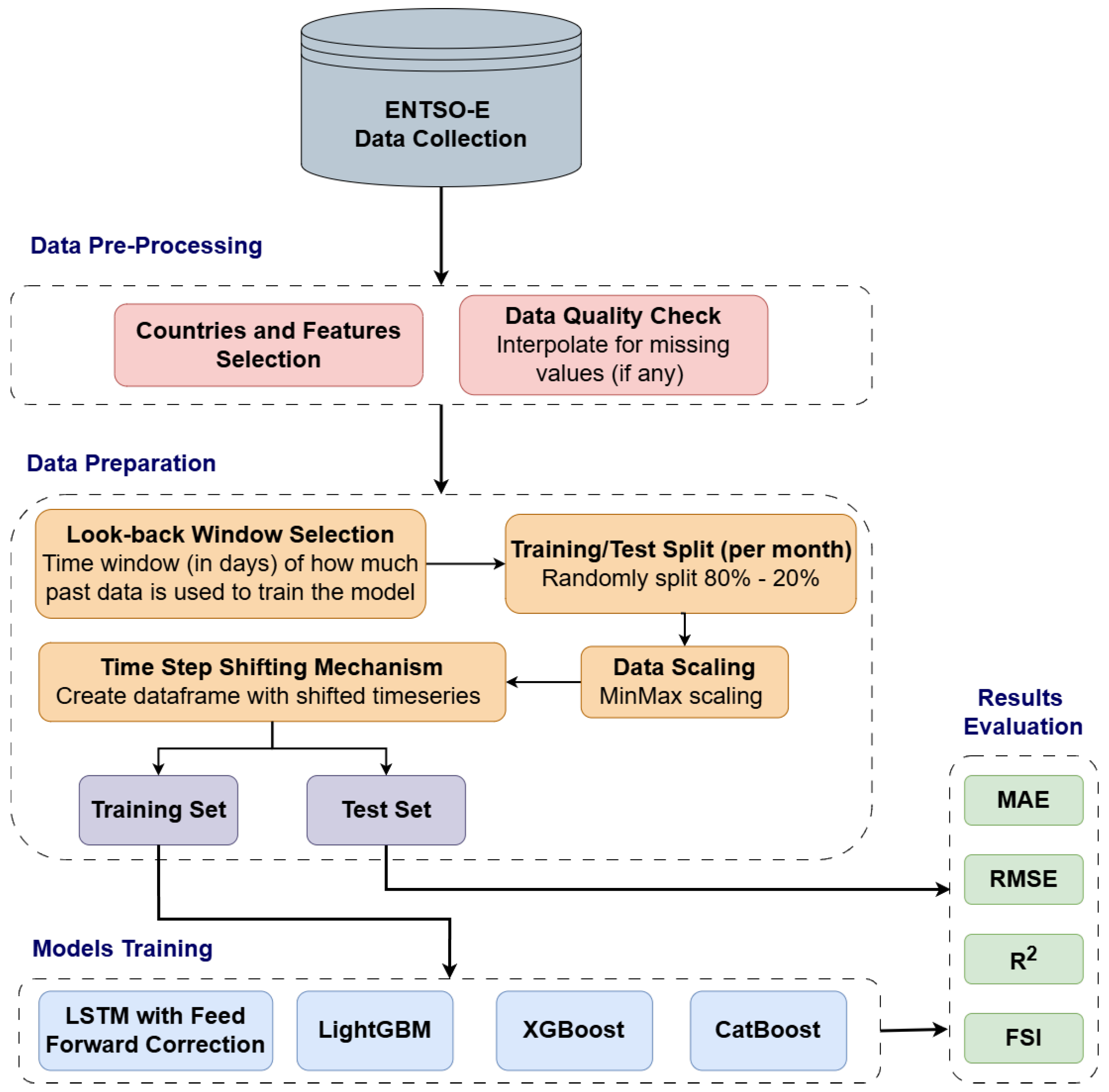
The modeling methodology and its main analytical stages are illustrated in Figure 1. Initially, data was collected using the European Network of TSOs for Electricity (ENTSO-E) Transparency Platform [27]. Historical DAM prices for the electricity markets of Greece, Belgium, and Ireland were collected for the 2023 calendar year. Historical forecast data for electricity demand, RES generation, total generation, and transmission net flows were also collected to serve as additional features aimed at improving DAM price prediction accuracy. Linear interpolation was applied in the case of missing values in both DAM prices and additional features. The decision to train the models using historical forecasted features corresponding to the DAM price prediction period, rather than actual values from the previous day, is motivated by two key factors: they reflect the system operators’ most up-to-date view of market conditions, and they are available at the time when market participants need to make their DAM price predictions.
The modeling pipeline differs from most related works due to the selection of various look-back windows and the decision to train and test models independently for each month of the year. More specifically, in this work, a thorough investigation of different look-back windows is performed, covering 7, 14, 30, 45, 60, and 90 days. These look-back windows define the amount of past data (in days) used to train and test the models. An 80% training and 20% test set split ratio applies to each month of the dataset, ensuring that enough historical data is available to match the selected look-back window. As a result, the earliest training date that can be randomly selected within a month depends on the window size, i.e., for a 45-day window, the earliest day used for training would be 15 February 2023. In the 45-day look-back window case, and for the longest look-back windows (e.g., 60 or 90 days), predictions for January–March cannot be conducted, depending on the number of past days needed for training.
Data normalization and time-step shifting are essential preprocessing steps before feeding the data into LSTM, LightGBM, XGBoost, and CatBoost models. To ensure consistency across features, MinMax scaling is applied independently to the training and test datasets, based on the transformation shown in Equations (1) and (2):
X norm = X min ( X ) max ( X ) min ( X ) , X χ
X scaled = X norm · ( L u p L l o w ) + L l o w , X χ
where χ represents the set of input features X, and { L l o w , L u p } are the lower and upper boundaries of the desired feature range. Figure 2 shows the time-step shifting mechanism applied in this work to create a time series of historical data, where n = 24 stands for the previous 24 hourly time steps.

2.2. Day-Ahead Market Price Forecasting Methods

The methodologies applied for the efficient execution of the experiment include several boosting models and an RNN.

2.2.1. Boosting Models

Boosting is an ML ensemble technique that creates several weak models sequentially, typically decision trees, trained to minimize the residual errors of the preceding models. The model is updated at each time step t, leading to a stronger model with improved accuracy based on the formula shown in Equation (3):
f t ( x ) = f t 1 ( x ) + α · l t ( x ) , α ( 0 , 1 ]
where f t ( x ) is the updated model at a time step t, l t ( x ) is the weak learner trained on the residual error of f t 1 ( x ) at time step t, while α is the learning rate. The Gradient Boosting is an extension to this technique and is also based on Equation (3), but instead of training each new weak learner on the residual errors of the previous model, the training occurs on the pseudo residual errors. These are simply the negative gradients of a chosen differentiable loss function per sample and are shown in Equation (4):
r i ( t ) = L ( y i , y ^ i ) y ^ i y ^ i = f t 1 ( x i )
where r i ( t ) is the pseudo-residual of the i t h sample at the time step t, L ( y i , y ^ i ) is the differentiable loss function, y i is the true target value for the i t h instance and y ^ i is the predicted value for the i t h instance.
XGBoost Model
XGBoost, which stands for Extreme Gradient Boosting, shares the same principles of gradient boosting shown in Equations (3) and (4) and performs a level-wise split of the nodes. In addition, instead of training each weak learner on the pseudo-residual errors of the last model, it adds the weak learner that minimizes a regularized objective function L ( t ) at each iteration, as shown in Equation (5), which incorporates both first and second-order derivatives of the loss function and a regularization term Ω ( l t ) that penalizes the complexity of the chosen weak learner, as shown in Equation (6):
L ( t ) = i = 1 n L ( y i , y ^ i ( t ) ) + Ω ( l t ) L ( y i , y ^ i ( t ) ) L ( y i , y ^ i ( t 1 ) ) + g i l t ( x i ) + 1 2 h i l t 2 ( x i )
Ω ( l t ) = γ T + 1 2 λ w j 2
where g i and h i are the gradient and Hessian, respectively, of the last model’s loss function; T is the number of leaves the weak learner has; λ is the L2 regularization term that helps avoid overfitting; γ is the weak learner complexity penalty; and w j is the weight of leaf j. In this way, the XGBoost model considers both the prediction accuracy and the model complexity for each iteration, offering more accurate and robust predictions.
CatBoost Model
With traditional gradient boosting, each weak learner is trained on residual errors from the same data the model was trained on, which causes potential data leakage, while categorical features must be encoded manually in order to be properly processed. Categorical Boosting (Catboost) aims to solve these problems by introducing ordered boosting and leak-free target-based encoding while splitting each node on the same feature with the same threshold, leading to symmetric trees. Specifically, instead of training each weak learner on the residual errors shown in Equation (4), it trains it on ordered pseudo-residual errors shown in Equation (7), where each residual per instance is computed based on the instances that preceded it in a given permutation σ .
r i ( t ) = L y i , f t 1 σ ( i ) 1 ( x i ) y ^ i
where σ ( i ) is the position of the instance i in the permutation and f t 1 σ ( i ) 1 ( x i ) is the prediction of the previous model trained on the first σ ( i ) 1 instances of the permutation. In addition, regarding categorical encoding, the CatBoost model replaces each instance of a categorical feature with the mean target value of the same category of preceding instances in a given permutation σ , as shown in Equation (8).
x ^ k i = x j D k 1 { x j i = x k i } · y j + a p x j D k 1 { x j i = x k i } + α
where x ^ k i is the encoding of the categorical feature i of instance k, D k = x j : σ ( j ) < σ ( k ) the set of instances before the instance k, p is the prior target value and α is a regularization constant controlling the influence of the prior target value. In summary, it extends the gradient boosting framework by effectively eliminating data leakage, improving generalization, and facilitating categorical feature encoding.
LightGBM Model
The Light Gradient Boosting Machine (LightGBM) follows the basic principles of gradient boosting and offers distinct advantages compared to the previous models. Initially, it optimizes the data through a pre-processing step that merges mutually exclusive features into a single feature to reduce dimensionality and performs leaf-wise node splitting based on the leaf with the highest loss reduction (gain). For the latter, it discretizes the continuous features into bins, and each one stores the sum of gradients and Hessians of the samples that fall into it, while the total calculation of the gain in a specific split point is shown in Equation (9):
G a i n ( s ) = G L ( s ) 2 H L ( s ) + λ + G R ( s ) 2 H R ( s ) + λ ( G L ( s ) + G R ( s ) ) 2 H L ( s ) + H R ( s ) + λ G L ( s ) = b s G b , H L ( s ) = b s H b G R ( s ) = b s G b , H R ( s ) = b s H b ,
where s is the split point, ( G b , H b ) are the sums of gradients and Hessians of all samples that fall into bin b, ( G L , H L ) are the total gradients and Hessians for all the bins less than or equal to bin s, ( G R , H R ) are the total gradients and Hessians for all the bins greater than bin s, and λ is the L2 regularization term on the leaf weights. Although this equation implies the use of the full dataset, this practice can be slow for large datasets and could hurt the accuracy of the model. For this reason, LightGBM performs non-uniform sampling by keeping the top a% of samples with the largest gradients and b % random samples from the rest and applies correction to their gradients and Hessians, as shown in Equation (10):
g i | h i g i | h i , if i large - gradient | hessian 1 a b · g i | h i , if i small - gradient | hessian
This way the model uses a subset of data for significantly reduced computational cost with adjusted gradients and Hessians to maintain unbiased estimations and increased efficiency.

2.2.2. Recurrent Neural Networks

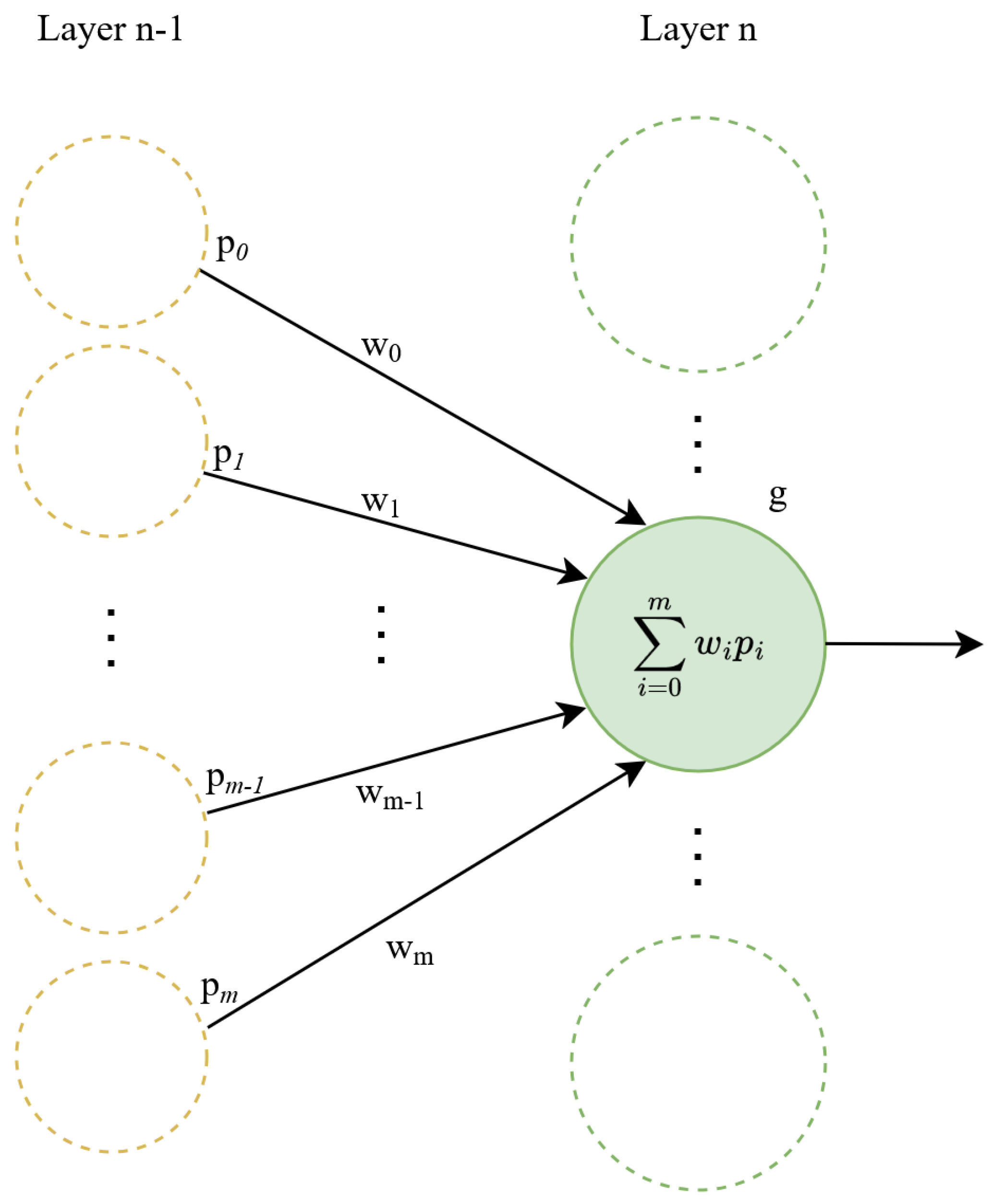
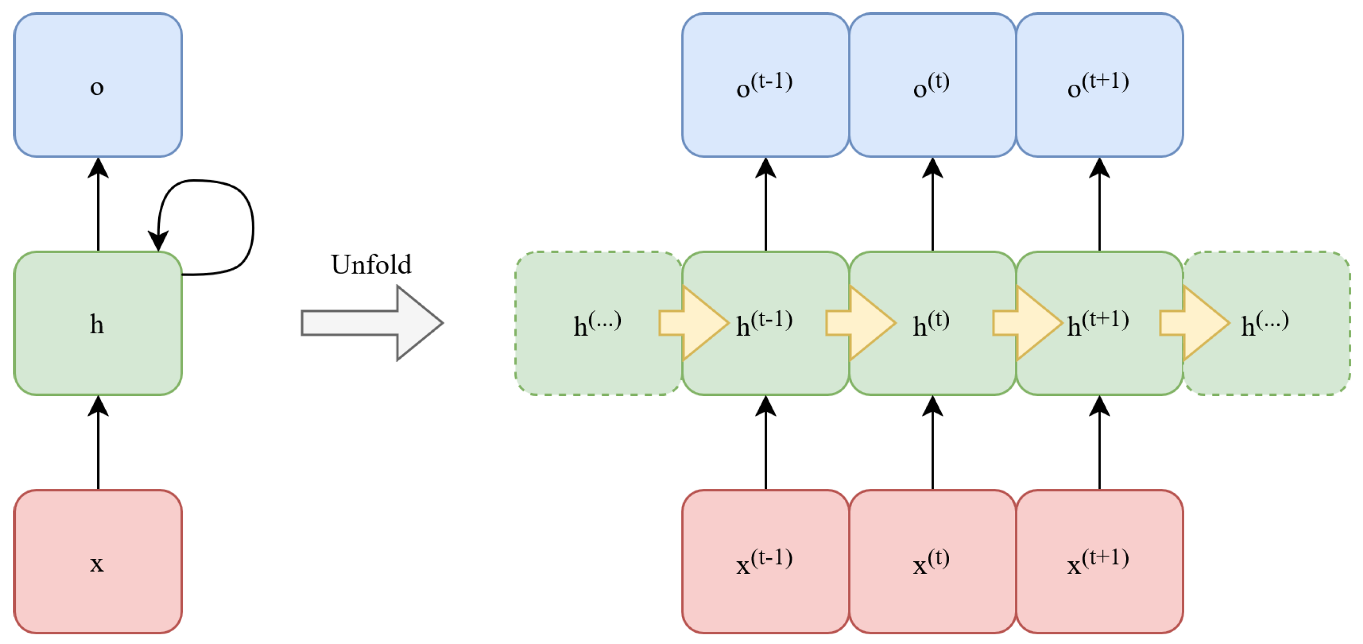
Aside from boosting models, artificial neural networks have transformed the forecasting industry by efficiently leveraging big data, leading to improved seasonal/trend detection and predictive accuracy. Their main difference from previous models lies in the simulation of layers of artificial neurons [28], connected through parameterized pathways that are learned through repetitive training, as shown in Figure 3. Where p i is the output of neuron i from the previous layer and w i is the weight of the pathway that links this neuron with neuron i of the previous layer. This structure facilitates the identification of complex patterns and dependencies in the data, while several architectures extended this design, such as RNNs, which have been the networks most widely used for sequence prediction problems [29]. Specifically, they were designed to handle sequential data and perform temporal modeling, while their recurrent nature can be attributed to an additional connection that transfers the output of a neuron at a specific time step t to itself as an additional input in the next time step t + 1 , called hidden state h t [30], as shown in Figure 4.
This way, the models can keep information from previous time steps to influence the forecasting process, but they are limited only to recent past information, are prone to overfitting, and suffer from the vanishing/exploding gradient problem.
Long Short-Term Memory with Feed-Forward Error Correction
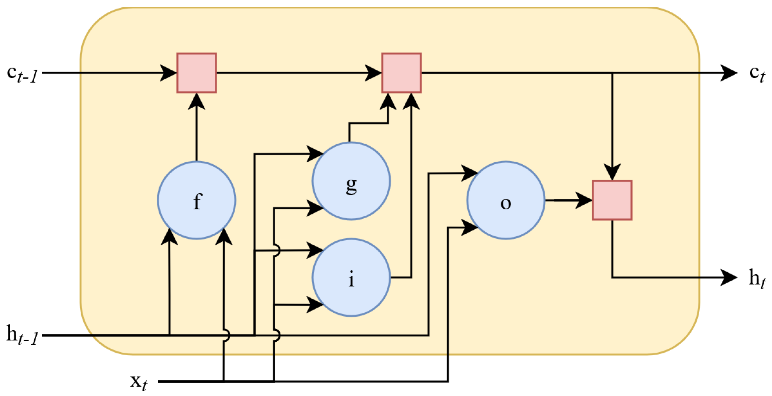
To solve these problems, an LSTM model with Feed-Forward Error Correction (FFEC) was developed. The LSTM architecture, originally introduced by [31] and subsequently enhanced by [32], is a specialized type of RNN, which introduced gating mechanisms that control the flow of information within the neuron and a second transferable state in addition to the hidden state, called the cell state c t [33], as shown in Figure 5.
The f represents the Forget Gate, which decides what part of the information from the previous cell state to forget, as shown in Equation (11). The g is the Candidate Cell State, which proposes new information to be potentially added to the cell state, as shown in Equation (12). The i is the Input Gate, responsible for the amount of information from the candidate cell state to add to the cell state, as shown in Equation (13), and the o is the Output Gate, which controls how much information from the cell state should be exposed and added to the hidden state, as shown in Equation (14). Additionally, the method of update for both states is shown in Equation (15)
f ( t ) = σ g ( W f x ( t ) + R f h ( t 1 ) + b f )
g ( t ) = σ c ( W g x ( t ) + R g h ( t 1 ) + b g )
i ( t ) = σ g ( W i x ( t ) + R i h ( t 1 ) + b i )
o ( t ) = σ g ( W o x ( t ) + R o h ( t 1 ) + b o )
c ( t ) = f ( t ) c ( t 1 ) + i ( t ) g ( t ) h ( t ) = o ( t ) σ ( c ( t ) )
where W i is the weight matrix applied to the input vector x ( t ) , R i is the recurrent weight matrix applied to the hidden state h ( t 1 ) , σ c is the activation function of the state, which is usually the hyperbolic tangent function, and σ g is the activation function of the gates, which is usually the sigmoid function.
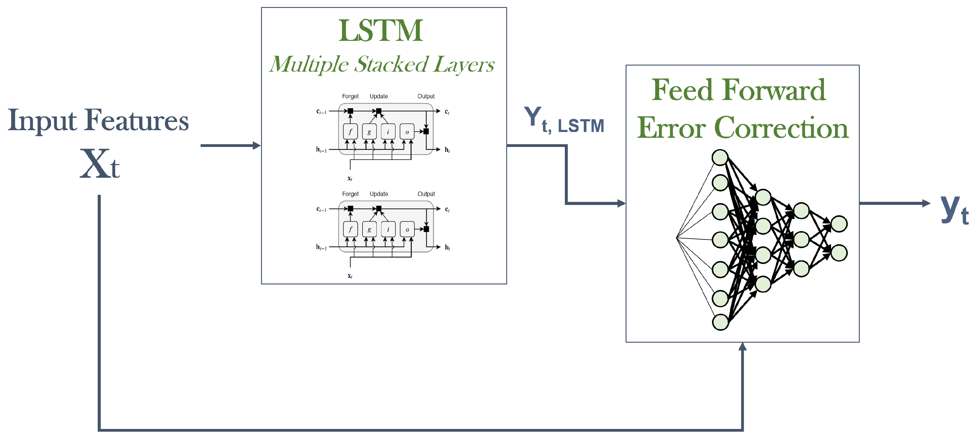
In this work, the typical LSTM architecture is integrated with a Feed-Forward Error Correction mechanism, inspired by the architecture proposed in Ref. [34]. The developed model is illustrated in Figure 6.
Specifically, the input features X t = [ x t n , , x t 3 , x t 2 , x t 1 ] are used to train the LSTM, which generates a preliminary prediction Y t , LSTM . This initial forecast is then refined using a Feed-Forward Neural Network (FFNN), which takes as input both the LSTM prediction and the historical data. The FFNN produces an improved estimate of DAM prices for the target time interval t. This two-stage approach aims to enhance the accuracy of predictions by leveraging the error correction capabilities of the FFNN.

2.3. European Market Structures

In recent years, the structure and functioning of short-term electricity markets have become increasingly aligned across different regions, with many jurisdictions adopting a similar framework [35], largely in response to the rising share of variable Renewable Energy Sources (RES) [36]. Accordingly, we illustrate the design of a typical European market by examining the configuration of one of the three examples mentioned in this manuscript—the Greek electricity market.
Over the past decade, the energy sector in Greece has undergone significant changes. These reforms encompass various aspects, such as the liberalization of the wholesale and retail electricity markets, allowing for greater competition. Furthermore, there has been a notable diversification of the electricity generation sources mix, with a significant rise in the proportion of variable RES contributing to the overall final energy consumption, reaching nearly 20% in 2019 [37] and 25% in 2023 [38]. Another noteworthy advancement is the transition to the new EU target model market. This includes the establishment of forward, DAM, and Intra-day Market (IDM) by the Hellenic Energy Exchange (HEnEx), as well as the introduction of a Balancing Market managed by the Independent Power Transmission Operator (IPTO-ADMIE), in accordance with the EU Target Model. A single distribution system operator, known as the Hellenic Electricity Distribution Network Operator (HEDNO), manages the distribution grid and the non-interconnected islands, whereas IPTO is responsible for the transmission grid. The energy market is overseen by the Regulatory Authority for Energy (RAE).
The current design of the Greek electricity market is characterized by a centralized framework for trading spot energy, along with separate market mechanisms dedicated to forward and “flexible” capacity trading, in line with the EU Target Model market structure, as follows:
  • The Forward Market (FM), managed by HEnEx, facilitates the exchange of forward contracts with either physical or financial settlement, typically on a monthly or annual basis. The Athens Exchange Clearing House (ATHEXClear) handles the clearing of these transactions.
  • DAM functions to equilibrate supply and demand for the following day.
    -
    It ensures that all wholesalers and retailers have access to the market and establishes reliable reference system prices (System Marginal Prices).
    -
    The primary tradable asset is an hourly electricity contract necessitating physical delivery, specifying unit-based price and volume.
    -
    A Day-Ahead Schedule (DAS) is generated by HEnEx, after solving the EU market price coupling, via an algorithm called EUPHEMIA [39].
  • IDM market allows participants to adjust their positions in close to real-time, particularly in situations involving changes in demand or supply. It also allows for the submission of more precise short-term forecasts for RES.
    -
    Hourly buy and sell orders are valid on the delivery day, commencing after the DAM window closes.
    -
    Prior to 21 September 2021, three local intra-day auctions were conducted within the Greek IDM.
    -
    Currently, the Greek IDM lacks implicit coupling with adjacent markets; consequently, cross-border capacity is not re-optimized post-DAM and remains unavailable for trading in this timeframe.
  • A distinct Balancing Market (BM), operated by IPTO, comes into play as we approach real-time operations, utilizing a simplified merit-order algorithm to activate Balancing Energy.
The BM can be seen as a flexibility trading market, ensuring system safety, as it has not only economic, but mainly physical effects. According to RAE [40], “the purpose of the Balancing Market is to correct the imbalance between production and demand in real time, maintaining the technical standards of the system and taking into account the results of the previous markets.”

3. Evaluation

3.1. Experimental Setup

In this study, we evaluate the performance of four distinct ML models: LSTM with FFEC, XGBoost, LightGBM, and CatBoost. Each model is configured with the respective hyperparameters, as summarized in Table 1.
The LSTM with FFEC model leverages recurrent layers to capture temporal dependencies in DAM price series, with FFEC layers refining predictions by correcting residual errors, addressing the specific limitations of LSTMs in short-window environments. Hyperparameters, such as moderate LSTM units, dropout, and MAE loss, were selected to balance learning capacity and overfitting, which is especially important for short training periods. For the tree-based models (XGBoost, LightGBM, and CatBoost), parameters like learning rate, tree depth, and subsampling were tuned to ensure stable learning and generalization from limited historical data.

3.2. Metrics

To effectively assess the performance of the models in the DA market, it is essential to measure and compare their respective error variances. To achieve this, a diverse set of widely used metrics has been employed to quantify and compare their accuracy. In this study, the evaluation metrics include the Mean Absolute Error, the Mean Absolute Percentage Error, the Root Mean Squared Error, the Coefficient of Determination ( R 2 ), and the Forecast Skill Index (FSI). Each of these metrics captures different aspects of predictive performance, providing complementary insights that contribute to a comprehensive evaluation. This section briefly describes these metrics along with their mathematical formulations.
The MAE is one of the most commonly used metrics, measuring the average absolute difference between predicted and actual values. It is scale-dependent, expressed as a single numerical value, and treats all errors equally, providing a general indication of a model’s performance. Its mathematical formulation is as follows:
M A E = 1 T t = 1 T p t a t
The MAPE, on the other hand, converts the mean absolute error into a percentage, offering a relative measure that is independent of scale. However, it may not always be fully comparable, as the denominator can vary significantly. Its equation is given by:
M A P E = 1 T t = 1 T p t a t a t × 100 %
The RMSE emphasizes larger errors by squaring the differences before averaging them, making it particularly useful for assessing a model’s robustness. A lower RMSE value indicates higher forecasting accuracy. The formula i as follows:
R M S E = 1 T t = 1 T ( p t a t ) 2
The R 2 score evaluates a model’s ability to explain the variance in actual energy production. It measures the proportion of variance captured by the forecasting model, with values ranging from 0 (no explanatory power) to 1 (perfect prediction). The formula is as follows:
R 2 = 1 t = 1 T ( p t a t ) 2 t = 1 T ( a ¯ a t ) 2
While these traditional error metrics—RMSE, MAE, MAPE, and R 2 —are widely used to evaluate forecasting models, they may not be sufficient when comparing models across different datasets, locations, or forecasting horizons [41]. In this context, the FSI provides an additional layer of evaluation by benchmarking model accuracy against a naive persistence model, confirming that the performance gap is systematic and not due to random variance. This approach ensures a more objective assessment of predictive capabilities. Mathematically, FSI is defined as follows:
F S I = 1 R M S E model R M S E persistence
where R M S E persistence corresponds to the relevant error of a naive persistence model, which assumes that future values remain unchanged from the most recent observed data. The choice of the reference model in forecast skill evaluation plays a crucial role in performance assessment, and in this study, the naive model is used as a baseline. Incorporating FSI alongside traditional error metrics provides a more well-rounded evaluation of forecasting accuracy in the DAM.

3.3. Cross-Model Comparative Analysis

In this study, five models were evaluated for DAM price forecasting: Naive, LSTM, XGBoost, LightGBM, and CatBoost. Table 2 presents the experimental results for each of the three countries across different training windows (7, 14, 30, 45, 60, and 90 days). In bold are the best metrics for each training window, and those assigned with are the optimal ones for all training windows for each country. As observed, LightGBM consistently outperforms the other models in nearly every metric and training window. Notably, it achieves lower MAE and RMSE values while maintaining high R 2 and FSI scores across all three countries. Moreover, LightGBM exhibits superior computational efficiency, with significantly lower training times compared to LSTM and other boosting models.
The impact of the training window size is evident, as increasing the training history generally leads to better model performance. This is reflected in the decreasing MAE and RMSE values and the increasing R 2 scores. Shorter training windows (7 and 14 days) tend to yield lower accuracy, whereas longer windows, particularly 90 days, result in more reliable forecasts. However, in some cases, the 60-day training window achieves better results than the 90-day window, especially for RMSE (e.g., Greece and Ireland for LightGBM). This suggests that while longer training windows generally improve forecasting performance, an optimal window length may exist, beyond which additional historical data introduces noise or reduces adaptability to recent market trends.
Among the other models, XGBoost and CatBoost perform well but consistently fall short of LightGBM. LSTM, on the other hand, struggles with shorter training windows, sometimes producing negative R 2 values (e.g., Greece, 7 days, R 2 = 0.104 ), indicating weak predictive performance. This suggests that while LSTMs are well-suited for sequential modeling, they may require extensive hyperparameter tuning and longer training histories to achieve competitive results.
The FSI further supports the superiority of LightGBM, as it achieves the highest FSI scores across most cases. The FSI values increase with the training window length, reinforcing the observation that more historical data leads to better forecasting accuracy. While XGBoost and CatBoost also show high FSI values, LightGBM remains the best-performing model overall. These findings confirm that LightGBM is the most effective and efficient approach for DAM price forecasting, highlighting the importance of training window selection in improving predictive performance.
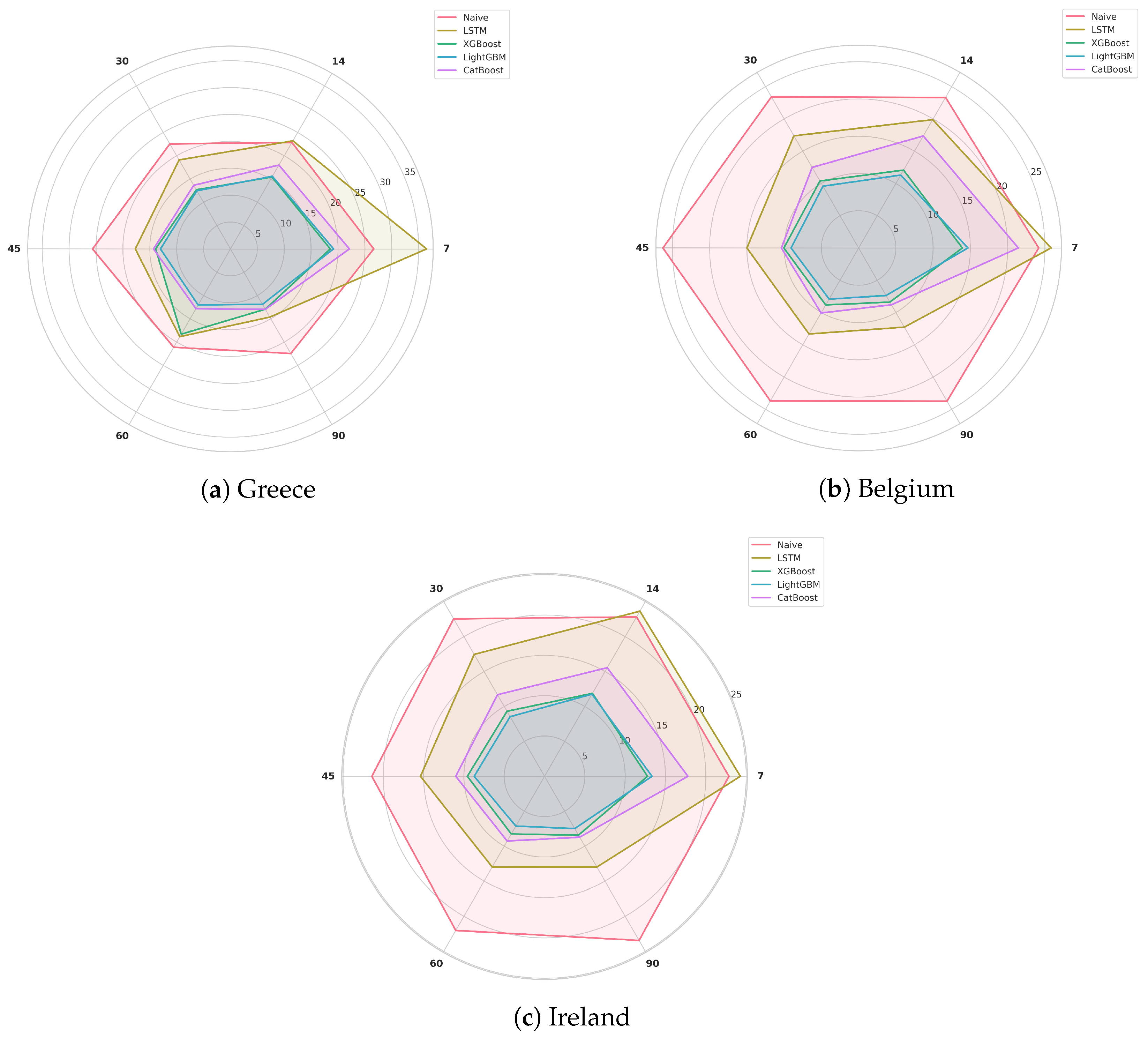
The radar plots in Figure 7 visually complement the results presented in Table 2, offering a clear comparison of model performance across different training windows for each country. The plots illustrate how the prediction error varies with different training periods, with lower values indicating better performance. LightGBM consistently achieves the lowest error in most cases, reinforcing its dominance in the tabular results. However, XGBoost and CatBoost also demonstrate competitive performance, particularly for longer training windows. Notably, in some instances, the 60-day training window yields better results than the 90-day window, suggesting that an optimal balance between training data size and model generalization exists. The plots further highlight the relatively weaker performance of LSTM and the Naive model, particularly for shorter training windows, emphasizing the superiority of gradient boosting methods for DAM price forecasting.

3.4. Seasonal and Market Price Spike Assessment

Electricity market prices are influenced by a variety of factors, including seasonal demand variations, supply constraints, and external economic conditions. In addition to evaluating model performance across different training windows, it is crucial to assess how well these models capture seasonal fluctuations and sudden price spikes. Such extreme price deviations can significantly impact market participants, necessitating models that not only provide accurate forecasts under normal conditions but also respond effectively to rapid market changes. This section analyzes the ability of the evaluated models to adapt to seasonal trends and predict extreme price movements, offering insights into their robustness and reliability in real-world scenarios.
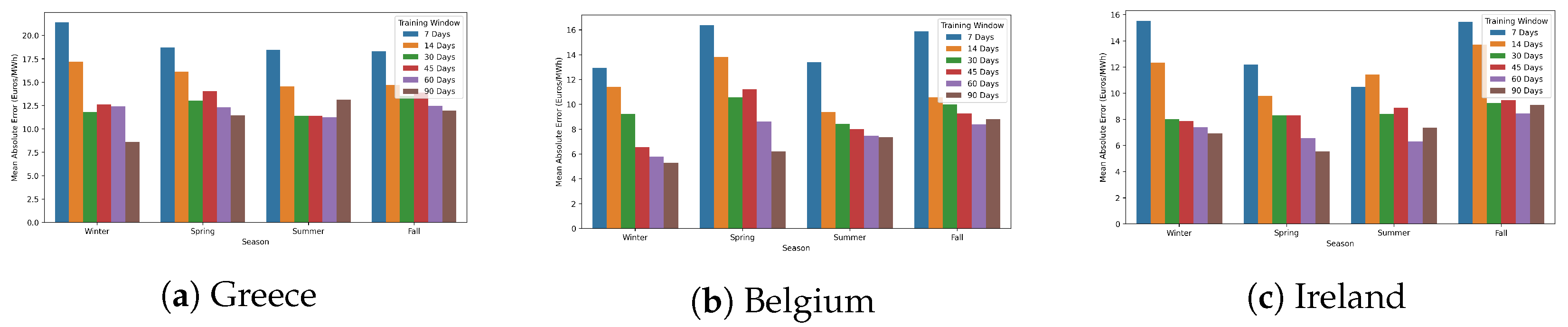
In Figure 8, the seasonal MAE plots provide insights into the influence of seasonality on forecasting accuracy across different training window lengths. In general, shorter training windows (e.g., 7 or 14 days) exhibit higher errors again, particularly during winter and spring, likely due to increased market volatility. Longer training windows (90 days) consistently demonstrate lower MAE across seasons for all countries, highlighting their ability to capture long-term trends.
In general, summer and fall are the seasons with the highest fluctuations in energy markets, driven by factors such as increased demand during hot temperatures, changes in energy production due to weather conditions, and shifts in supply from RES. These fluctuations are particularly pronounced during peak consumption periods, making accurate forecasting critical for market participants. Interestingly, the 45-day and 60-day training windows tend to outperform the 90-day window in these seasons. The 90-day window incorporates a broader range of data, including less relevant or outdated trends that might not accurately reflect the current market dynamics. As the energy market responds more strongly to short-term fluctuations in demand and supply, the shorter 45-day and 60-day windows are better able to capture these seasonal variations and provide more responsive predictions. These results emphasize the importance of seasonality in selecting appropriate forecasting strategies.
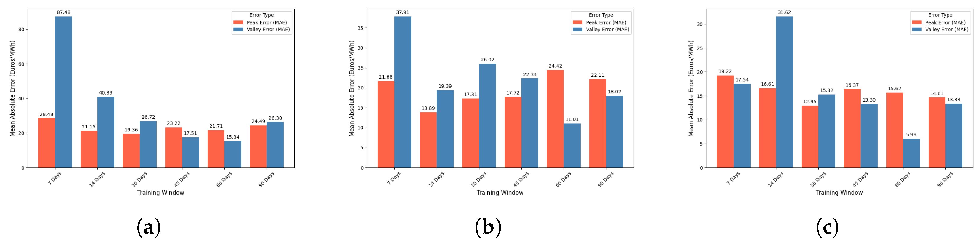
Delving deeper into our analysis, it becomes evident that the choice of training window significantly impacts the accuracy of peak and valley predictions across different countries. As illustrated in Figure 9, both Greece and Belgium exhibit notably higher errors with the 7-day window, especially for valley predictions, reflecting the insufficiency of shorter training periods in capturing complex market behaviors. In contrast, the 45-day and 60-day training windows consistently yield lower MAE values for both peak and valley forecasts, indicating a more balanced responsiveness to recent trends without the dilution effect seen in the 90-day window. This pattern is particularly clear in countries like Greece, where the 30- and 60-day windows achieve the lowest peak error of all configurations. These findings reinforce the hypothesis that medium-range training windows—specifically 45 and 60 days—strike an optimal balance by incorporating relevant, recent market data while excluding outdated information, thereby enhancing the forecasting model’s adaptability to seasonal volatility and sudden market shifts typical of summer and fall periods.

4. Conclusions and Outlook

Concluding, accurate forecasting of DAM electricity prices is critical for the efficient operation of power systems and the financial planning of market participants. As the growing share of RES and increased cross-border trading amplify market volatility, this paper contributes by evaluating ML approaches across Greece, Belgium, and Ireland using shallow training windows. For traders and VPP operators, the identified optimal 45–60 day window offers a practical mechanism to manage financial risk by adapting quickly to structural market breaks without the latency of deep historical training. Similarly, TSOs can leverage these computationally efficient models for rapid deployment in data-scarce environments, although the approach remains constrained by its reliance on forecasted feature availability and shows reduced efficacy during extremely short (7-day) data windows.
More specifically, through a comprehensive evaluation of an LSTM with FFEC, XGBoost, LightGBM, and CatBoost models over varying restricted training windows (7, 14, 30, 45, 60, and 90 days), we identified clear patterns in model performance and data sensitivity. The findings highlight that LightGBM consistently outperforms other models in terms of both accuracy and computational efficiency, especially when using medium-range training windows (45 to 60 days). These windows strike an optimal balance between capturing relevant historical trends and avoiding the inclusion of outdated or noisy data, as reflected in both overall error metrics and the models’ ability to predict seasonal fluctuations and price spikes. Furthermore, the importance of careful data pre-processing is underscored. The use of forecasted features from ENTSO-E, rather than actual historical values, provided models with realistic inputs aligned with operational forecasting conditions. Historical forecast data for electricity demand, RES generation, total generation, and transmission net flows were also collected to serve as additional features, aiming at improving DAM price prediction accuracy. Additionally, time-step shifting proved critical for preparing datasets, particularly for models sensitive to input scale and temporal sequences.
Looking ahead, as the EU moves toward a more interconnected and decarbonized energy system, forecasting approaches will need to support greater spatial granularity, shorter decision-making cycles, and alignment with regulatory frameworks promoting transparency and flexibility. Moreover, future developments must focus on quantifying uncertainty through probabilistic forecasting methods to provide explicit confidence intervals for risk-averse decision-making. Investment in scalable, adaptive ML systems will be crucial to meeting these emerging needs, enabling stakeholders to navigate an increasingly dynamic electricity landscape with confidence whilst increasing both profitability and sustainability.

Author Contributions

Conceptualization, V.M. and C.M.-A.; methodology, V.M., C.M.-A. and E.S.; software, V.M. and C.M.-A.; validation, V.M. and C.M.-A.; formal analysis, V.M., C.M.-A. and A.Z.; investigation, V.M. and C.M.-A.; resources, P.S.G., D.A. and E.S.; data curation, V.M. and C.M.-A.; writing—original draft preparation, V.M., C.M.-A., E.S., A.Z., P.S.G. and D.A.; writing—review and editing, V.M., C.M.-A., E.S., A.Z., P.S.G. and D.A.; visualization, V.M. and C.M.-A.; supervision, P.S.G. and D.A.; project administration, P.S.G. and D.A.; funding acquisition, P.S.G. and D.A. All authors have read and agreed to the published version of the manuscript.

Funding

The work presented is based on research conducted within the framework of the Horizon Europe European Commission project CRETE VALLEY (Grant Agreement No. 101136139). The content of the paper is the sole responsibility of its authors and does not necessary reflect the views of the EC.

Data Availability Statement

Conflicts of Interest

The authors declare no conflict of interest.

Abbreviations

The following abbreviations are used in this manuscript:
AIArtificial Intelligence
ANNArtificial Neural Network
ARIMAAutoRegressive Integrated Moving Average
BMBalancing Market
CNNConvolutional Neural Network
DAMDay-Ahead Market
DLDeep Learning
DNNDeep Neural Network
FMForward Market
FFECFeed-Forward Error Correction
FSIForecast Skill Index
GRUGated Recurrent Unit
IDMIntra-day Market
LSTMLong Short-Term Memory
MAEMean Absolute Error
MAPEMean Absolute Percentage Error
MLMachine Learning
MSEMean Squared Error
PVPhotovoltaic
RNNRecurrent Neural Network
RMSERoot Mean Squared Error
SVRSupport Vector Regression
TFTTemporal Fusion Transformer
VPPVirtual Power Plant

References

  1. MacIver, C.; Bell, K.R.; Adam, G.P.; Xu, L. Electrical interconnectors: Market opportunities, regulatory issues, technology considerations and implications for the GB energy sector. Energy Strategy Rev. 2021, 38, 100721. [Google Scholar] [CrossRef] [Scilit]
  2. Manfre Jaimes, D.; Zamudio López, M.; Zareipour, H.; Quashie, M. A hybrid model for multi-day-ahead electricity price forecasting considering price spikes. Forecasting 2023, 5, 499–521. [Google Scholar] [CrossRef] [Scilit]
  3. Shimomura, M.; Keeley, A.R.; Matsumoto, K.; Tanaka, K.; Managi, S. Beyond the merit order effect: Impact of the rapid expansion of renewable energy on electricity market price. Renew. Sustain. Energy Rev. 2024, 189, 114037. [Google Scholar] [CrossRef] [Scilit]
  4. Kazemtarghi, A.; Mallik, A.; Chen, Y. Dynamic pricing strategy for electric vehicle charging stations to distribute the congestion and maximize the revenue. Int. J. Electr. Power Energy Syst. 2024, 158, 109946. [Google Scholar] [CrossRef] [Scilit]
  5. Ovaere, M.; Kenis, M.; Van den Bergh, K.; Bruninx, K.; Delarue, E. The effect of flow-based market coupling on cross-border exchange volumes and price convergence in Central Western European electricity markets. Energy Econ. 2023, 118, 106519. [Google Scholar] [CrossRef] [Scilit]
  6. Islam, M.M.; Yu, T.; Giannoccaro, G.; Mi, Y.; La Scala, M.; Nasab, M.R.; Wang, J. Improving reliability and stability of the power systems: A comprehensive review on the role of energy storage systems to enhance flexibility. IEEE Access 2024, 12, 152738–152765. [Google Scholar] [CrossRef] [Scilit]
  7. Papias, I.; Michalakopoulos, V.; Sarmas, E.; Marinakis, V.; Antonesi, G.; Cioara, T.; Anghel, I. A Data-Driven Framework for Estimating Residential Energy Flexibility for Aggregated Demand-Side Management. Sustain. Energy Grids Netw. 2025, 43, 101783. [Google Scholar] [CrossRef] [Scilit]
  8. Michalakopoulos, V.; Sarmas, E.; Papias, I.; Skaloumpakas, P.; Marinakis, V.; Doukas, H. A machine learning-based framework for clustering residential electricity load profiles to enhance demand response programs. Appl. Energy 2024, 361, 122943. [Google Scholar] [CrossRef] [Scilit]
  9. Michalakopoulos, V.; Papias, I.; Sarantinopoulos, E.; Sarmas, E.; Marinakis, V.; Askounis, D. A hyperparameter-space clustering methodology of residential electricity loads. Appl. Soft Comput. 2025, 181, 113497. [Google Scholar] [CrossRef] [Scilit]
  10. Li, L.; Fan, Y.; Tse, M.; Lin, K.Y. A review of applications in federated learning. Comput. Ind. Eng. 2020, 149, 106854. [Google Scholar] [CrossRef] [Scilit]
  11. Michalakopoulos, V.; Spyropoulos, L.; Ilias, L.; Sarmas, E.; Marinakis, V.; Askounis, D. A comparative analysis of federated learning strategies for short-term photovoltaic power forecasting. Energy Rep. 2025, 13, 4223–4235. [Google Scholar] [CrossRef] [Scilit]
  12. Nowotarski, J.; Weron, R. Recent advances in electricity price forecasting: A review of probabilistic forecasting. Renew. Sustain. Energy Rev. 2018, 81, 1548–1568. [Google Scholar] [CrossRef] [Scilit]
  13. Michalakopoulos, V.; Zakynthinos, A.; Sarmas, E.; Marinakis, V.; Askounis, D. Hybrid short-term wind power forecasting model using theoretical power curves and temporal fusion transformers. Renew. Energy 2025, 256, 124008. [Google Scholar] [CrossRef] [Scilit]
  14. Oprea, S.V.; Bâra, A. Analyzing Shock Transmission and Spillover Effect in the Day-Ahead and Intraday Markets: Key Implications for Price Forecasting. J. Knowl. Econ. 2025, 16, 17226–17265. [Google Scholar] [CrossRef] [Scilit]
  15. Tschora, L.; Pierre, E.; Plantevit, M.; Robardet, C. Electricity price forecasting on the day-ahead market using machine learning. Appl. Energy 2022, 313, 118752. [Google Scholar] [CrossRef] [Scilit]
  16. Lago, J.; Marcjasz, G.; De Schutter, B.; Weron, R. Forecasting day-ahead electricity prices: A review of state-of-the-art algorithms, best practices and an open-access benchmark. Appl. Energy 2021, 293, 116983. [Google Scholar] [CrossRef] [Scilit]
  17. Bozlak, Ç.B.; Yaşar, C.F. An optimized deep learning approach for forecasting day-ahead electricity prices. Electr. Power Syst. Res. 2024, 229, 110129. [Google Scholar] [CrossRef] [Scilit]
  18. Tan, Y.Q.; Shen, Y.X.; Yu, X.Y.; Lu, X. Day-ahead electricity price forecasting employing a novel hybrid frame of deep learning methods: A case study in NSW, Australia. Electr. Power Syst. Res. 2023, 220, 109300. [Google Scholar] [CrossRef] [Scilit]
  19. Li, J.; Zhang, C.; You, P.; Yin, S.; Lu, Y.; Li, C. A Hybrid GRU-LightGBM Model for Day-Ahead Electricity Price Forecasting. In Proceedings of the 2024 3rd International Conference on Energy and Electrical Power Systems (ICEEPS), Guangzhou, China, 14–16 July 2024; pp. 630–634. [Google Scholar] [CrossRef] [Scilit]
  20. Mubarak, H.; Abdellatif, A.; Ahmad, S.; Zohurul Islam, M.; Muyeen, S.; Abdul Mannan, M.; Kamwa, I. Day-Ahead electricity price forecasting using a CNN-BiLSTM model in conjunction with autoregressive modeling and hyperparameter optimization. Int. J. Electr. Power Energy Syst. 2024, 161, 110206. [Google Scholar] [CrossRef] [Scilit]
  21. Kitsatoglou, A.; Georgopoulos, G.; Papadopoulos, P.; Antonopoulos, H. An ensemble approach for enhanced Day-Ahead price forecasting in electricity markets. Expert Syst. Appl. 2024, 256, 124971. [Google Scholar] [CrossRef] [Scilit]
  22. Yorat, E.; Zor, K.; Özbek, N.S.; Sarıbulut, L. Day-ahead electricity price forecasting using artificial intelligence-based algorithms. In Proceedings of the 2023 International Conference on Innovation and Intelligence for Informatics, Computing, and Technologies (3ICT), Sakheer, Bahrain, 20–21 November 2023; pp. 121–126. [Google Scholar] [CrossRef] [Scilit]
  23. Sun, C.; Pan, X.; Li, G.; Li, P.; Gao, G.; Tian, Y.; Xu, G. Day-Ahead Electricity Price Forecasting Strategy Based on Machine Learning and Optimization Algorithm. In Proceedings of the 2022 4th Asia Energy and Electrical Engineering Symposium (AEEES), Chengdu, China, 25–28 March 2022; pp. 254–259. [Google Scholar] [CrossRef] [Scilit]
  24. Micu, R.; Tudose, A.; Iantoc, A.; Picioroaga, I.; Bulac, C. Electricity Price Forecasting on Day Ahead Market via a Multivariate CNN-LSTM Model. In Proceedings of the 2024 IEEE International Conference and Exposition on Electric and Power Engineering (EPEi), Iași, Romania, 17–19 October 2024; pp. 611–615. [Google Scholar] [CrossRef] [Scilit]
  25. Pavićević, M.; Popović, T. Forecasting Day-Ahead Electricity Price with Artificial Neural Networks: A Comparison of Architectures. In Proceedings of the 2021 11th IEEE International Conference on Intelligent Data Acquisition and Advanced Computing Systems: Technology and Applications (IDAACS), Cracow, Poland, 22–25 September 2021; Volume 2, pp. 1083–1088. [Google Scholar] [CrossRef] [Scilit]
  26. Nitsch, F.; Schimeczek, C.; Bertsch, V. Applying machine learning to electricity price forecasting in simulated energy market scenarios. Energy Rep. 2024, 12, 5268–5279. [Google Scholar] [CrossRef] [Scilit]
  27. ENTSO-E. Transparency Platform. 2024. Available online: https://transparency.entsoe.eu/ (accessed on 10 December 2024).
  28. Meyer-Baese, A.; Schmid, V. Chapter 7–Foundations of Neural Networks. In Pattern Recognition and Signal Analysis in Medical Imaging, 2nd ed.; Meyer-Baese, A., Schmid, V., Eds.; Academic Press: Oxford, UK, 2014; pp. 197–243. [Google Scholar] [CrossRef] [Scilit]
  29. Hewamalage, H.; Bergmeir, C.; Bandara, K. Recurrent Neural Networks for Time Series Forecasting: Current status and future directions. Int. J. Forecast. 2021, 37, 388–427. [Google Scholar] [CrossRef] [Scilit]
  30. Das, S.; Tariq, A.; Santos, T.; Kantareddy, S.S.; Banerjee, I. Recurrent Neural Networks (RNNs): Architectures, Training Tricks, and Introduction to Influential Research. In Machine Learning for Brain Disorders; Colliot, O., Ed.; Springer: New York, NY, USA, 2023; pp. 117–138. [Google Scholar] [CrossRef] [Scilit]
  31. Hochreiter, S.; Schmidhuber, J. Long Short-Term Memory. Neural Comput. 1997, 9, 1735–1780. [Google Scholar] [CrossRef] [Scilit]
  32. Gers, F.A.; Schmidhuber, J.A.; Cummins, F.A. Learning to forget: Continual prediction with LSTM. Neural Comput. 2000, 12, 2451–2471. [Google Scholar] [CrossRef] [Scilit] [PubMed]
  33. MathWorks. Long Short-Term Memory Neural Networks. Available online: https://www.mathworks.com/help/deeplearning/ug/long-short-term-memory-networks.html (accessed on 1 May 2025).
  34. Menos-Aikateriniadis, C.; Akarepis, A.; Kokos, I.; Georgilakis, P.S. Sub-Hourly Load Forecasting for Community-Level Flexible Appliance Management. In Proceedings of the 2024 International Joint Conference on Neural Networks (IJCNN), Yokohama, Japan, 30 June–5 July 2024; pp. 1–8. [Google Scholar] [CrossRef] [Scilit]
  35. Newbery, D.; Strbac, G.; Viehoff, I. The benefits of integrating European electricity markets. Energy Policy 2016, 94, 253–263. [Google Scholar] [CrossRef] [Scilit]
  36. Silva-Rodriguez, L.; Sanjab, A.; Fumagalli, E.; Virag, A.; Gibescu, M. Short term wholesale electricity market designs: A review of identified challenges and promising solutions. Renew. Sustain. Energy Rev. 2022, 160, 112228. [Google Scholar] [CrossRef] [Scilit]
  37. Forouli, A.; Bakirtzis, E.A.; Papazoglou, G.; Oureilidis, K.; Gkountis, V.; Candido, L.; Ferrer, E.D.; Biskas, P. Assessment of Demand Side Flexibility in European Electricity Markets: A Country Level Review. Energies 2021, 14, 2324. [Google Scholar] [CrossRef] [Scilit]
  38. European Commission. Renewable Energy Statistics. 2023. Available online: https://ec.europa.eu/eurostat/statistics-explained/index.php?title=Renewable_energy_statistics (accessed on 8 May 2025).
  39. EnEx Group. Market’s Coupling—Price Coupling of Regions (PCR). 2024. Available online: https://www.enexgroup.gr/pcr (accessed on 23 September 2024).
  40. Regulatory Authority for Energy (RAE). Balancing Market. 2024. Available online: https://www.ceer.eu/wp-content/uploads/2024/04/C21_NR_Greece_EN.pdf (accessed on 23 September 2024).
  41. Koutsandreas, D.; Spiliotis, E.; Petropoulos, F.; Assimakopoulos, V. On the selection of forecasting accuracy measures. J. Oper. Res. Soc. 2022, 73, 937–954. [Google Scholar] [CrossRef] [Scilit]
Figure 1. Proposed methodology for Day-Ahead Market price forecasting under different look-back windows and a monthly training/test set split.
Energies 19 00376 g001
Figure 2. Time Step Shifting Mechanism for training/test time series creation.
Energies 19 00376 g002
Figure 3. An artificial neuron architecture.
Energies 19 00376 g003
Figure 4. A simple RNN neuron (left) and its unrolled form over sequential time steps (right).
Energies 19 00376 g004
Figure 5. The architecture of an LSTM neuron.
Energies 19 00376 g005
Figure 6. LSTM with Feed-Forward Error Correction architecture.
Energies 19 00376 g006
Figure 7. Radar plots comparing model performance across different training windows (7, 14, 30, 45, 60, and 90 days) for Greece, Belgium, and Ireland. Each axis represents a training window, and lower values indicate better performance.
Energies 19 00376 g007
Figure 8. Seasonal MAE for different training windows across Greece, Belgium, and Ireland.
Energies 19 00376 g008
Figure 9. Peak analysis for different countries: (a) Greece, (b) Belgium, and (c) Ireland.
Energies 19 00376 g009
Table 1. Hyperparameter settings for all models considered.
ModelHyperparameterValue
LSTM with FFECLSTM, FFEC Optimizersadam
LSTM Units200
LSTM Dropout Rate0.2
LSTM Learning Rate 1 × 10 4
LSTM, FFEC Loss FunctionsMAE
LSTM, FFEC Epochs200
LSTM, FFEC Batch Sizes256
FFEC Layer 1, 2 Sizes256, 128
FFEC Activations (1, 2)ReLU
XGBoostLoss FunctionMSE
Colsample Bytree0.9
Learning Rate0.01
Tree Maximum Depth10
Number of Trees300
Tree Subsample0.8
LightGBMObjectiveRegression
Colsample Bytree0.9
Learning Rate0.01
Maximum Depth10
Number of Trees300
Subsample0.8
CatBoostObjectiveRMSE
Learning Rate0.01
Depth10
Iterations500
Subsample0.8
Random Seed42
Table 2. Modeling results.
TrainingWindowEvaluationMetricsGREECEBELGIUMIRELAND
Naive LSTM XGB LGBM CatBoost Naive LSTM XGB LGBM CatBoost Naive LSTM XGB LGBM CatBoost
7 daysMAE26.65136.47718.56119.16722.12324.17125.83813.93014.67721.44822.87024.29012.77313.33717.787
RMSE39.72252.22927.62827.78733.91834.66734.53820.79221.42431.00833.80832.48619.00419.32325.347
R 2 0.361−0.1040.6910.6870.5340.4370.4410.7980.7850.5510.3580.4070.7970.7900.639
FSI0−0.3150.3040.3000.14600.0040.4000.3820.10600.0390.4380.4280.250
14 daysMAE22.86423.20515.44515.59918.01023.33919.89212.06911.30017.36122.82123.64711.88311.76515.552
RMSE34.13331.53222.98022.22928.05033.71426.55018.67717.48026.25632.76336.75119.50218.83725.004
R 2 0.4080.4950.7320.7490.6000.4650.6680.8360.8550.6740.4280.2800.7970.8110.667
FSI00.0760.3270.3490.17800.2120.4460.4820.2210−0.1220.4050.4250.237
30 daysMAE22.54619.10412.70012.48913.66323.42017.38210.3839.57712.48722.54617.4559.3148.53811.682
RMSE33.46329.14219.27318.65321.25133.34824.07417.75615.70321.25032.59923.40314.07712.90018.258
R 2 0.2920.4630.7650.7800.7140.4590.7180.8470.8800.7810.2490.6130.8600.8820.765
FSI00.1290.4240.4430.36500.2780.4680.5290.36300.2820.5680.6040.440
45 daysMAE25.64817.69813.92813.02014.31126.27414.99810.0379.07210.37421.41915.3919.5778.72611.012
RMSE37.82025.98420.87319.29922.20436.86720.48916.19314.44117.69930.74221.37515.54413.89418.526
R 2 0.1090.5790.7290.7680.6930.2550.7710.8570.8870.8170.4230.7210.8520.8820.790
FSI00.3130.4480.4900.41300.4440.5610.6090.52100.3050.4940.5480.397
60 daysMAE21.12118.83918.30312.03012.82723.70213.3248.8307.92110.07522.02312.9828.2537.1239.273
RMSE30.25541.73912.39917.49219.25233.88518.63114.15312.45717.09831.56918.12612.78010.91714.627
R 2 0.338−0.2600.7580.7790.7320.3470.8030.8860.9120.8340.3870.7980.9000.9270.868
FSI0−0.3800.3950.4220.36400.4500.5820.6320.49500.4260.5950.6540.537
90 daysMAE22.45414.63612.94911.89912.97923.73912.2698.3857.3658.80623.45112.9898.4237.4858.719
RMSE34.51922.19920.65817.89121.16535.63418.32314.36812.80515.19533.75618.37413.30011.70114.111
R 2 0.3200.7190.7560.8170.7440.2600.8040.8800.9040.8650.1440.7460.8670.8970.850
FSI00.3570.4020.4820.38700.4860.5970.6410.57400.4560.6060.6530.582
Disclaimer/Publisher’s Note: The statements, opinions and data contained in all publications are solely those of the individual author(s) and contributor(s) and not of MDPI and/or the editor(s). MDPI and/or the editor(s) disclaim responsibility for any injury to people or property resulting from any ideas, methods, instructions or products referred to in the content.