Residential Electricity-Use Profiling for Demand-Side Management Using a Convolutional Attention Variational Autoencoder and Adaptive GWO-K-Means Clustering

Abstract

Residential load profiling can support the design of differentiated demand-side management, but clustering methods are sensitive to representation quality and initialization. We developed a profiling workflow that combines a convolutional attention variational autoencoder (CA-VAE), adaptive gray wolf optimizer K-Means (GWO-K-Means) search over candidate cluster numbers and centers, and a clustering-loss refinement stage. On 6390 prepared residential average-day load profiles from the Commission for Energy Regulation dataset, ten independent runs yielded a final silhouette coefficient of 0.5002 (SD 0.0314), a Davies–Bouldin index of 0.8532 (SD 0.0383), and a Calinski–Harabasz index of 3694.3 (SD 260.5). Relative to raw K-Means, the final workflow improved all three internal validity measures (paired Wilcoxon signed-rank test, p = 0.001953 for each metric). GWO selected K = 5 in 6 of 10 runs; this modal solution produced five interpretable load profiles. The profiles provide load-shape-derived candidate groups for future demand-response trials, rather than validated estimates of operational flexibility.

1. Introduction

Residential demand is increasingly important to power-system flexibility because household loads collectively shape distribution-network peaks and the effectiveness of time-of-use tariffs and demand-response programs. Smart-meter data make it possible to segment users according to recurring load shapes and to match groups with differentiated demand-side management interventions [1,2,3]. However, residential smart-meter data are high-dimensional, large-scale, variable in quality, and characterized by nonlinear relationships [4]. Electricity-use patterns also differ substantially among households, leading to heterogeneous load-regulation potential [5]. Reliable user profiling therefore requires methods that distinguish behaviorally meaningful load shapes while retaining a clear connection to operational energy-management decisions.

Clustering algorithms group users with similar electricity-use patterns [6,7] and can be broadly categorized as direct or indirect methods. Direct clustering applies an algorithm directly to electricity-consumption data. Improved K-Means and fuzzy C-means remain widely used for classifying daily load curves [8,9]. Dynamic time warping combined with density-peak clustering has also been used to identify typical load curves [10,11], and state-feature clustering has been applied to non-intrusive load-event detection [12]. Nevertheless, direct clustering often cannot capture complex behavioral variation in high-dimensional electricity data, which limits clustering performance.

Indirect clustering extracts lower-dimensional features before clustering. Common approaches include manually designed indicators and dimensionality-reduction algorithms. Indicators such as daily maximum load and load factor can characterize electricity use [13], but they provide limited information about temporal evolution. Principal component analysis has been applied to user-metering data [14], but its linear formulation cannot adequately represent nonlinear relationships. Dimensionality reduction has also been combined with ensemble clustering for load-curve analysis [15]. More recently, deep-learning methods have been introduced into load clustering [16]. A joint convolutional neural network autoencoder (CNN-AE) and hierarchical clustering model has shown the potential of deep feature extraction and joint training for electricity-use pattern classification [17]. Long short-term memory autoencoders have also been studied [18], although their requirement for a single continuous input series makes simultaneous classification of multiple users difficult. Recent Energies research has further combined ensemble clustering with explainable artificial intelligence to connect residential load profiles with demand-response decisions [19], highlighting the importance of both clustering performance and operational interpretability.

Despite these advances, deep learning-based feature extraction still has three limitations. First, conventional convolutional autoencoders capture local temporal features but do not explicitly model long-range dependencies across a load curve. Second, clustering algorithms such as K-Means require the number of clusters and initial cluster centers to be specified in advance and are sensitive to local optima. Third, most methods separate feature extraction from clustering, so the learned representation is not necessarily aligned with the clustering objective.

This study develops a residential load-profiling workflow that combines convolutional attention variational representation learning with adaptive GWO-K-Means and clustering-loss refinement. Its contribution is not the use of any component in isolation. Instead, it evaluates a reproducible sequence in which CA-VAE produces compact daily load embeddings, GWO searches candidate values of K and initial centers using a pre-specified SC-DBI objective, and a subsequent clustering-loss stage is assessed rather than being assumed to improve the representation. The framework targets 48-step average-day profiles and preserves direct profile-level interpretation. The empirical claims are limited to internal clustering validity on the CER dataset and screening-level demand-side management implications.

2. Data Preprocessing

2.1. Data Source

The present analysis uses a prepared CER input matrix [20] containing 6390 user-level, Min–Max normalized average daily load curves with 48 half-hourly values per user. The retained input is complete and contains no NaN or Inf values. The analysis therefore focuses on clustering these supplied long-term average-day profiles.

Averaging daily load curves emphasizes persistent shape characteristics but suppresses day-specific, seasonal, and weekday–weekend variation. The conclusions are consequently limited to long-term shape-based residential profiling.

2.2. Scope of the Retained Input Data

The retained analysis file does not include the original day-level missingness pattern or raw daily records. We therefore do not claim a new validation of the mean value of simultaneous data (MVSD) imputation in this revision. Comparing MVSD with alternative imputation methods requires the original daily observations and is identified as future work.

For a user with a missing observation at a given time, the imputed value is calculated as follows:

$$x_t^{(i)}={\displaystyle \frac{1}{N}}{\displaystyle \sum _{j\in \mathrm{\Omega }}{x}_{j,t}^{(i)}}$$

(1)

where the missing measurement of the user at the target time is estimated from the set of valid days for the same user and the same time period; the denominator denotes the number of valid days in this set.

2.3. Normalization and Interpretation

Because the retained input does not include original day-level observations or anomaly labels, this revision does not re-evaluate a repeated 3-sigma outlier procedure or its effect on legitimate peak-demand behavior. Such validation requires raw daily data and observed event labels.

$${\mu }_i={\displaystyle \frac{1}{M}}{\displaystyle \sum _{m=1}^M{x}_m^{(i)}}$$

(2)

$${\sigma }_i=\sqrt{{\displaystyle \frac{1}{M}}{\displaystyle \sum _{m=1}^M{(x_m^{(i)}-{\mu }_i)}^2}}$$

(3)

where the mean, standard deviation and number of valid measurement points are calculated for each user. Then, each measurement is judged according to the following criterion:

$$|x_m^{(i)}-{\mu }_i|>3{\sigma }_i\Rightarrow x_m^{(i)} \mathrm{is} \mathrm{outlier}$$

(4)

Detected outliers are treated as missing observations and imputed using MVSD. This procedure is repeated until no additional outliers are detected.

The supplied profiles are Min–Max normalized per user. This removes absolute load magnitude from the clustering input and emphasizes shape. Where original-scale profiles are used for interpretation, they are descriptive rather than part of the clustering objective.

$${\widehat{x}}_t^{(i)}={\displaystyle \frac{x_t^{(i)}-x_{{\min }^{(i)}}}{x_{{\max }^{(i)}}-x_{{\min }^{(i)}}}}$$

(5)

where each raw observation is normalized using the minimum and maximum observations for the same user. In the limiting case of a constant load, the denominator is set to 1 to avoid division by zero.

After normalization, each user’s average daily load curve lies in [0, 1], and the resulting matrix is used as the input to CA-VAE.

3. CA-VAE Feature Extraction Model

3.1. Basic Principle of Variational Autoencoder

A variational autoencoder (VAE) is a generative model that combines deep learning with probabilistic inference [21]. Unlike a conventional autoencoder (AE), a VAE imposes a probability distribution, typically a standard normal distribution, on the latent variables, producing a more regular and continuous latent representation.

A VAE comprises an encoder and a decoder. The encoder maps the input to the mean and log-variance parameters of the latent posterior distribution. Using the reparameterization trick, the decoder samples a latent variable from this distribution and reconstructs the input. Maximizing the evidence lower bound (ELBO) is equivalent to minimizing the following loss function:

$$L_{\mathrm{VAE}}=L_{\mathrm{recon}}+\beta \cdot L_{\mathrm{KL}}$$

(6)

The reconstruction loss measures the discrepancy between the input and reconstructed output. This study uses mean squared error (MSE):

$$L_{\mathrm{recon}}={\displaystyle \frac{1}{n}}{\displaystyle \sum _{i=1}^n\Vert x_i-{\widehat{x}}_i{\Vert }^2}$$

(7)

where the batch size, the original normalized load sequence and the load sequence reconstructed by the decoder are used to calculate the reconstruction error.

KL divergence regularizes the latent posterior distribution toward the prior distribution:

$$L_{\mathrm{KL}}=-{\displaystyle \frac{1}{2}}{\displaystyle \sum _{j=1}^d(1+\log {\sigma }_j^2-{\mu }_j^2-{\sigma }_j^2)}$$

(8)

where the calculation uses the latent-space dimension and the mean and standard deviation produced by the encoder. KL divergence prevents the latent space from degenerating into a deterministic mapping and promotes continuity and diversity in the learned representation.

The weighting coefficient balances reconstruction quality against latent-space regularization. A larger value produces a more regular latent space at the cost of reconstruction accuracy, whereas a smaller value improves reconstruction but may reduce latent-space smoothness. Its value is selected experimentally.

3.2. Encoder Structure Integrating Convolution and Attention

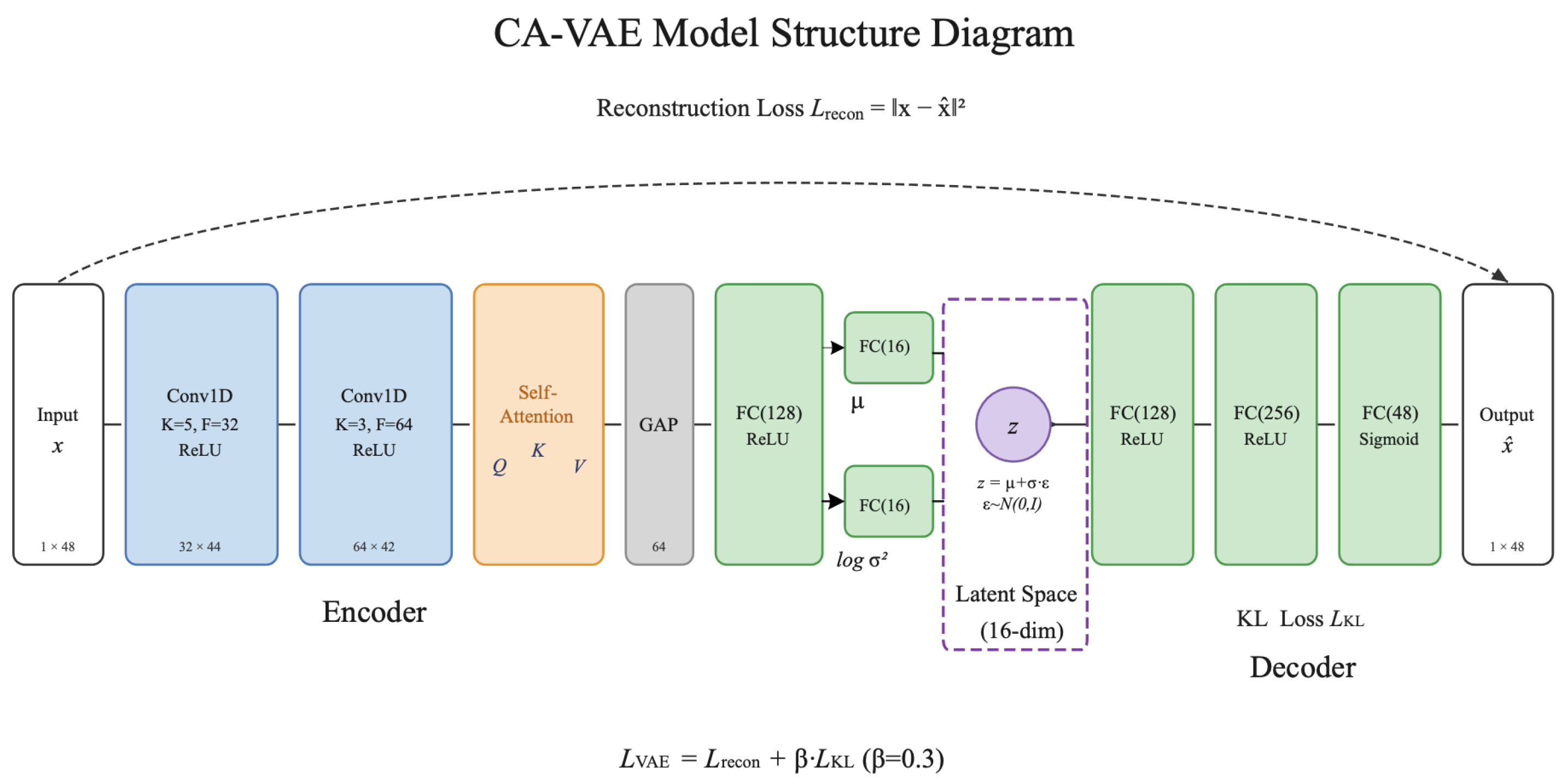
To improve VAE feature extraction for electricity-use time series, the encoder is extended with convolution and attention. As shown in Figure 1, the resulting convolutional attention encoder comprises one-dimensional convolutional layers, a self-attention layer, and fully connected layers.

(1) One-dimensional convolutional neural network (1D-CNN). A 1D-CNN applies a sliding window along the time series to extract local temporal features. Two one-dimensional convolutional layers are used here to learn increasingly abstract temporal patterns.

First convolutional layer: the normalized 48-dimensional load sequence is treated as a one-channel signal. Each kernel spans five consecutive half-hour periods (2.5 h) to capture short-term load variation. The convolution reduces the temporal dimension from 48 to 44 and is expressed as follows:

$$h_t^{(1,f)}=\mathrm{ReLU}\left({\displaystyle \sum _{k=0}^{K_1-1}{W}_k^{(1,f)}}\cdot x_{t+k}+b^{(1,f)}\right),\hspace{1em}t=1,\dots ,T_1$$

(9)

where the output of the first-layer filter at each time step is determined by the corresponding convolution weights, bias term and activation function.

The second convolutional layer extracts higher-level temporal patterns from the multichannel feature maps produced by the first layer. This convolution reduces the temporal dimension from 44 to 42 and is expressed as follows:

$$h_t^{(2,f)}=\mathrm{ReLU}\left({\displaystyle \sum _{k=0}^{K_2-1}{\displaystyle \sum _{c=1}^{F_1}{W}_{k,c}^{(2,f)}}}\cdot h_{t+k}^{(1,c)}+b^{(2,f)}\right),\hspace{1em}t=1,\dots ,T_2$$

(10)

where the output is determined by the second-layer filter weights across time offsets and input channels. Together, the two convolutional layers learn a hierarchy of temporal representations, from local 2.5 h trends to higher-level combinations of load patterns.

(2) Self-attention layer. Convolutional layers capture local temporal dependencies but do not directly model relationships between distant time periods. A self-attention mechanism is therefore introduced after the convolutional layers [17]. Three learnable linear transformations map the convolutional feature matrix to query, key, and value matrices, from which attention weights between time steps are calculated:

$$Q=H{W}_Q,\hspace{1em}K=H{W}_K,\hspace{1em}V=H{W}_V$$

(11)

The attention weights are obtained using scaled dot-product attention:

$$\mathrm{Attention}(Q,K,V)=\mathrm{softmax}\left({\displaystyle \frac{Q{K}^T}{\sqrt{d_k}}}\right)V$$

(12)

The attention-weight matrix quantifies how strongly each time step attends to every other time step during encoding. This mechanism is well suited to residential electricity-use data, which often contain dependencies across distant periods, such as low daytime consumption followed by concentrated evening demand or high nighttime heating demand followed by low daytime demand. Such relationships extend beyond the local receptive field of a convolution kernel. Self-attention can encode these long-range dependencies, thereby improving the distinction between latent representations of different electricity-use patterns.

For example, the mechanism can associate low electricity use at 08:00 with high electricity use at 18:00, a pattern consistent with residents being away during the day and returning in the evening.

(3) Global average pooling and fully connected layers. Global average pooling (GAP) compresses the feature matrix produced by the attention layer into a fixed-length vector by averaging along the temporal dimension:

$$\overline{h}={\displaystyle \frac{1}{T_2}}{\displaystyle \sum _{t=1}^{T_2}{h}_t^{\mathrm{attn}}}$$

(13)

where the 64-dimensional feature vector at each time step is averaged across all time steps after the second convolution. Because GAP retains information from the full daily sequence, it is suitable for representing complete load-curve shapes. The resulting 64-dimensional vector is mapped to a 128-dimensional intermediate representation, after which two linear layers produce the mean and log-variance of the latent variables:

$$h_{fc}=\mathrm{ReLU}(\overline{h}{W}_{fc}+b_{fc})$$

(14)

$$\mu =h_{fc}{W}_{\mu }+b_{\mu }$$

(15)

$$\log {\sigma }^2=h_{fc}{W}_{\sigma }+b_{\sigma }$$

(16)

Reparameterization: sampling directly from the posterior distribution is not differentiable and therefore prevents encoder optimization by backpropagation. The reparameterization trick is used to address this problem [21]:

$$z=\mu +\exp (0.5\cdot \log {\sigma }^2)\cdot ϵ,\hspace{1em}ϵ~\mathcal{N}(0,I)$$

(17)

where a random vector is sampled from a standard normal distribution. This transformation isolates the stochastic component from the model parameters, allowing gradients to propagate through the mean and variance parameters to the encoder.

3.3. Decoder Structure

The decoder reconstructs the original 48-dimensional load curve from the 16-dimensional latent variable z. It uses a three-layer fully connected architecture: z (16 dimensions) → FC (128) → FC (256) → FC (48). The first two layers use ReLU activation, and the final layer produces the reconstructed load curve. A Sigmoid activation constrains the output to [0, 1], matching the normalized input range.

$$\widehat{x}=\sigma (d_2{W}_{d3}+b_{d3})$$

(18)

$$\hspace{1em}\sigma (x)={\displaystyle \frac{1}{1+e^{-x}}}$$

(19)

3.4. Training Strategy

CA-VAE is pretrained with Adam for 200 epochs using a learning rate of 0.002, a KL-divergence weight beta of 0.3, batch size 256, a 16-dimensional latent space, convolution kernels of 5 and 3, and 32 and 64 filters. Gradients are clipped at 5. These values were fixed for the repeated-run study; gamma, fitness weights, and attention were additionally examined through the robustness checks reported below.

4. Adaptive Clustering Based on GWO-K-Means

4.1. Basic Principle of Gray Wolf Optimizer

The gray wolf optimizer (GWO) is a swarm-intelligence algorithm inspired by the hunting behavior of gray wolves [22]. The population is organized into α, β, δ, and ω wolves, representing the best, second-best, third-best, and remaining candidate solutions, respectively. At each iteration, candidate positions are updated using the positions of the three leading wolves and progressively approach the optimum. The search comprises global exploration, encircling, and local exploitation.

Once a candidate prey location has been identified, the wolves update their positions to encircle it. This behavior is modeled as follows:

$$\overrightarrow{D}=|\overrightarrow{C}\cdot {\overrightarrow{X}}_p(t)-\overrightarrow{X}(t)|$$

(20)

$$\overrightarrow{X}(t+1)={\overrightarrow{X}}_p(t)-\overrightarrow{A}\cdot \overrightarrow{D}$$

(21)

where the formulation uses the current iteration, the prey position (the current best solution), the current wolf position, and the distance between the wolf and the prey. The coefficient vectors are calculated as follows:

$$vecA=2\overrightarrow{a}\cdot {\overrightarrow{r}}_1-\overrightarrow{a}$$

(22)

$$\overrightarrow{C}=2\cdot {\overrightarrow{r}}_2$$

(23)

where two random vectors are sampled uniformly from [0, 1]. The convergence factor decreases linearly from 2 to 0 over the optimization process according to the following expression:

$$a=2\left(1-{\displaystyle \frac{t}{T_{\max }}}\right)$$

(24)

where the maximum number of iterations is 80. As the convergence factor decreases from 2 to 0, the range of the coefficient vector contracts from [−2, 2] to [0, 0]. An absolute coefficient value greater than 1 promotes global exploration, whereas a value below 1 promotes local exploitation.

Because the true global optimum is unknown, the α, β, and δ wolves are treated as the most informative candidate solutions. Each wolf first calculates candidate positions relative to these three leaders:

$${\overrightarrow{X}}_1={\overrightarrow{X}}_{\alpha }-{\overrightarrow{A}}_1\cdot |{\overrightarrow{C}}_1\cdot {\overrightarrow{X}}_{\alpha }-\overrightarrow{X}|$$

(25)

$${\overrightarrow{X}}_2={\overrightarrow{X}}_{\beta }-{\overrightarrow{A}}_2\cdot |{\overrightarrow{C}}_2\cdot {\overrightarrow{X}}_{\beta }-\overrightarrow{X}|$$

(26)

$${\overrightarrow{X}}_3={\overrightarrow{X}}_{\delta }-{\overrightarrow{A}}_3\cdot |{\overrightarrow{C}}_3\cdot {\overrightarrow{X}}_{\delta }-\overrightarrow{X}|$$

(27)

The updated position of a wolf is then calculated as the mean of the three candidate positions:

$$\overrightarrow{X}(t+1)={\displaystyle \frac{{\overrightarrow{X}}_1+{\overrightarrow{X}}_2+{\overrightarrow{X}}_3}{3}}$$

(28)

where the three leaders are the first-, second-, and third-ranked individuals in the current population, and their coefficient vectors are generated independently. Combining information from all three leaders reduces reliance on a single best candidate and is intended to limit premature convergence.

4.2. Adaptive Optimization of K-Means Parameters Based on GWO

Adaptive GWO-K-Means searches K in [3, 10] and corresponding latent-space centers. Each wolf encodes a candidate K and its K centers. This range spans a minimum coarse distinction among residential shapes while limiting the number of profiles to an interpretable operational scale.

$$f=w_1\cdot \mathrm{SC}-w_2\cdot \mathrm{DBI}$$

(29)

The GWO fitness function is F = 0.6 SC − 0.4 DBI, where SC is maximized and DBI is minimized. CH is calculated as an independent third evaluation metric and is not added to the search objective, avoiding a second manually weighted composite criterion. In a controlled fixed-representation sensitivity check, four weight pairs from (0.3, 0.7) to (0.7, 0.3) all selected K = 5 and produced the same partition.

$$\mathrm{CH}={\displaystyle \frac{\mathrm{SSB}/(K-1)}{\mathrm{SSW}/(n-K)}}$$

(30)

$$SSB={\displaystyle \sum _{k=1}^K|}{C}_k|\cdot {\Vert {\mu }_k-\mu \Vert }^2$$

(31)

$$SSW={\displaystyle \sum _{k=1}^K{\displaystyle \sum _{z_i\in C_k}}}{\Vert z_i-{\mu }_k\Vert }^2$$

(32)

where SSB and SSW denote between-cluster and within-cluster dispersion, respectively. The calculation also uses the samples and center of each cluster and the global center across all samples. A larger CH value indicates stronger clustering performance. CH is not included in the fitness function and is used only as a third evaluation dimension.

The GWO population contains 30 wolves and is evolved for 80 iterations. Each candidate undergoes 10 local K-Means refinement iterations, and the K-mutation probability is 0.1. These settings were fixed before the repeated-run study to balance population exploration, local center refinement, and computational cost. The retained global-best candidate and its K trajectory are reported for reproducibility.

4.3. Selection Basis of K

To assess the K selected by GWO, the sum of squared errors (SSE), SC, DBI, and CH are calculated for each candidate value from K = 3 to K = 10. Figure 2 shows how the four indices vary with K.

As shown in Figure 2a, SSE decreases monotonically with increasing K, with a clear change in slope at K = 5. This elbow suggests that additional clusters beyond K = 5 provide diminishing reductions in within-cluster error. SC reaches its maximum of approximately 0.515 at K = 4, decreases to approximately 0.45 at K = 5, and rises to approximately 0.49 for K ≥ 7 (Figure 2b). DBI reaches its minimum of approximately 0.82 at K = 9 and is approximately 0.90 at K = 5 (Figure 2c), whereas CH generally increases with K and reaches its maximum at K = 10 (Figure 2d).

The validity indices can favor different values of K, especially because DBI and CH may favor more finely divided partitions. Across ten independent end-to-end runs, GWO selected K = 5 in 6 runs, K = 6 in 2 runs, and K = 9 in 2 runs. We therefore retain K = 5 as the modal, representative, and operationally interpretable solution, rather than as a unique numerical optimum. All selected K values are reported in the Supplementary Material.

For an additional comparison across K values, the four indices are transformed using Min–Max normalization. DBI and SSE are reversed so that larger normalized values consistently represent better performance. A weighted comprehensive score is then calculated, as shown in Figure 3.

Figure 3 shows distinct behavior among the four normalized indices. Normalized SC is highest at K = 4, whereas normalized DBI, CH, and SSE increase with K, causing the comprehensive score to generally rise as K increases. Because this trend is largely driven by indices that favor larger K, a higher comprehensive score alone does not establish that a larger number of clusters is more useful in practice.

Considering Figure 2 and Figure 3 together with the GWO fitness result, K = 5 provides a balanced solution across the validity indices. The resulting five profiles are also interpretable in terms of electricity-use periods and load levels and remain manageable for fine-grained demand-side management. K = 5 is therefore selected as the final number of clusters.

5. Joint Optimization Training

5.1. Basic Idea of the Joint Model

Conventional indirect clustering treats feature extraction and clustering as sequential, independent tasks. Feature extraction minimizes reconstruction error, whereas clustering minimizes classification error, with no feedback between the two objectives [17]. Consequently, the learned latent representation may not be well aligned with the clustering task.

To align these objectives, multitask learning is used to jointly optimize CA-VAE feature extraction and GWO-K-Means clustering. A clustering-loss term is added to the CA-VAE objective so that the encoder learns to reconstruct the input while also improving cluster structure. Clustering-loss gradients fine-tune the encoder, preserving salient load information while promoting within-cluster compactness and between-cluster separation. 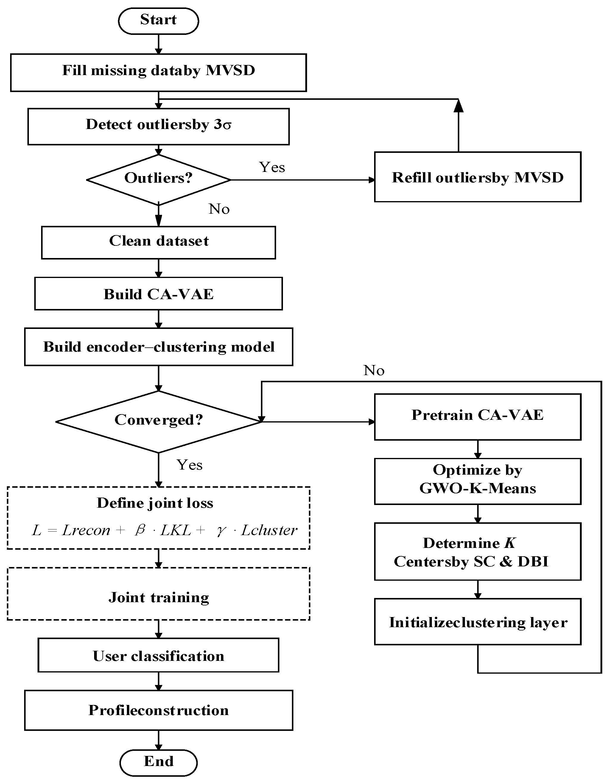Figure 4 shows the joint framework.

5.2. Clustering-Loss Function

Following the deep embedded clustering (DEC) method in [23], a custom clustering layer is added after the CA-VAE encoder. The layer weights represent cluster-center vectors and are initialized using the optimal centers obtained by GWO-K-Means.

The clustering layer converts latent-space distance into similarity. It first calculates the Euclidean distance between each user’s latent representation and each cluster center, then converts the distance into a soft assignment probability using the Student t-distribution:

$$q_{ij}={(1+{\Vert z_i-{\mu }_j\Vert }^2)}^{-1}/{\displaystyle \sum _{j^{\prime }=1}^K{(1+{\Vert z_i-{\mu }_{j^{\prime }}\Vert }^2)}^{-1}}$$

(33)

where the latent-space feature vector of a user, the coordinate vector of a cluster center and the probability that the user belongs to a cluster are considered.

Soft assignment retains each sample’s probability of belonging to every cluster, which is useful for samples near cluster boundaries. The Student t-distribution is used instead of a Gaussian distribution because its heavier tails assign relatively greater probability to samples farther from a cluster center. This property provides more balanced assignments at moderate latent-space distances and reduces excessive concentration in a small number of high-density regions [23].

In addition to the soft assignment distribution q, the clustering loss requires an auxiliary target distribution. This target strengthens high-confidence assignments while suppressing ambiguous assignments near cluster boundaries and is defined as follows:

$$p_{ij}=(q_{ij}^2/f_j)/{\displaystyle \sum _{j^{\prime }}(q_{i{j}^{\prime }}^2/f_{j^{\prime }})}$$

(34)

$$f_j={\displaystyle \sum _{i=1}^n{q}_{ij}}$$

(35)

where the auxiliary probability of a user belonging to a cluster is normalized by that cluster’s soft frequency across all samples, preventing large clusters from dominating the loss.

The auxiliary target distribution squares the soft assignment probabilities. This transformation increases the relative weight of high-confidence assignments and reduces the relative weight of low-confidence assignments, progressively sharpening the distribution and improving cluster discrimination.

The clustering loss is then defined as the KL divergence between the soft assignment distribution and the auxiliary target distribution:

$$L_{\mathrm{cluster}}=KL(p\Vert q)=(1/n){\displaystyle \sum _{i=1}^n{\displaystyle \sum _{j=1}^K{p}_{ij}}}\cdot \ln (p_{ij}/q_{ij})$$

(36)

Minimizing this divergence guides the encoder toward latent-space features for which the soft assignment approaches the target distribution, promoting compactness within clusters and separation between clusters.

5.3. Joint Loss Function and Training Process

The CA-VAE reconstruction loss, latent-space KL regularization, and clustering loss are combined in the joint objective:

$$L=L_{\mathrm{recon}}+\beta \cdot L_{\mathrm{KL}}+\gamma \cdot L_{\mathrm{cluster}}$$

(37)

where reconstruction loss measures the difference between the decoder output and the original input, latent-space KL regularization constrains the posterior distribution, and clustering KL divergence optimizes cluster assignment. The two weighting coefficients balance latent-space regularization and clustering loss.

Training proceeds in two stages. CA-VAE is pretrained for 200 epochs, then jointly refined for 80 epochs using one fifth of the pretraining learning rate. A fixed-seed gamma sensitivity check over {0, 0.05, 0.10, 0.20} retained K = 5 in all conditions; gamma = 0.05 had the best SC and DBI in that representative check. The clustering-loss stage is therefore evaluated as a refinement mechanism, not presumed to improve every internal metric.

Joint training updates the encoder and decoder parameters without repeating GWO. For the representative seed-42 solution, the GWO-selected K is 5; in the repeated study, K remains a stochastic search outcome and all selected values are retained in the analysis.

5.4. Experimental Configuration and Reproducibility

Ten independent end-to-end runs used seeds 42–51. Each run used the same data size, architecture, K search range, and baseline settings. MATLAB R2023a Update 7 with Statistics and Machine Learning Toolbox and Deep Learning Toolbox was run on a MacBook Air with an Apple M5 10-core CPU, 16 GB memory, and macOS 26.5.1; gpuDeviceCount was zero. The complete workflow including evaluated baselines required 4123.3 (SD 334.5) s. Mean durations of pretraining, GWO search, and joint refinement were 2185.5, 313.6, and 1276.9 s, respectively.

6. Results and Discussion

The complete residential user clustering workflow is shown in Figure 4:

(1) Impute missing values, detect outliers, and normalize the raw CER records to obtain a cleaned input matrix;

(2) Pretrain CA-VAE on the processed electricity-use data for 200 epochs to obtain initial latent-space feature vectors;

(3) Apply adaptive GWO-K-Means in the latent space using 30 wolves and 80 iterations to determine K and the initial cluster-center vectors;

(4) Initialize the clustering layer with the GWO-K-Means solution and jointly train feature extraction and clustering for 80 epochs using clustering-loss feedback;

(5) Extract the final latent representation, assign users to cluster centers, and construct a profile for each cluster.

6.1. Training Behavior and Cluster Selection

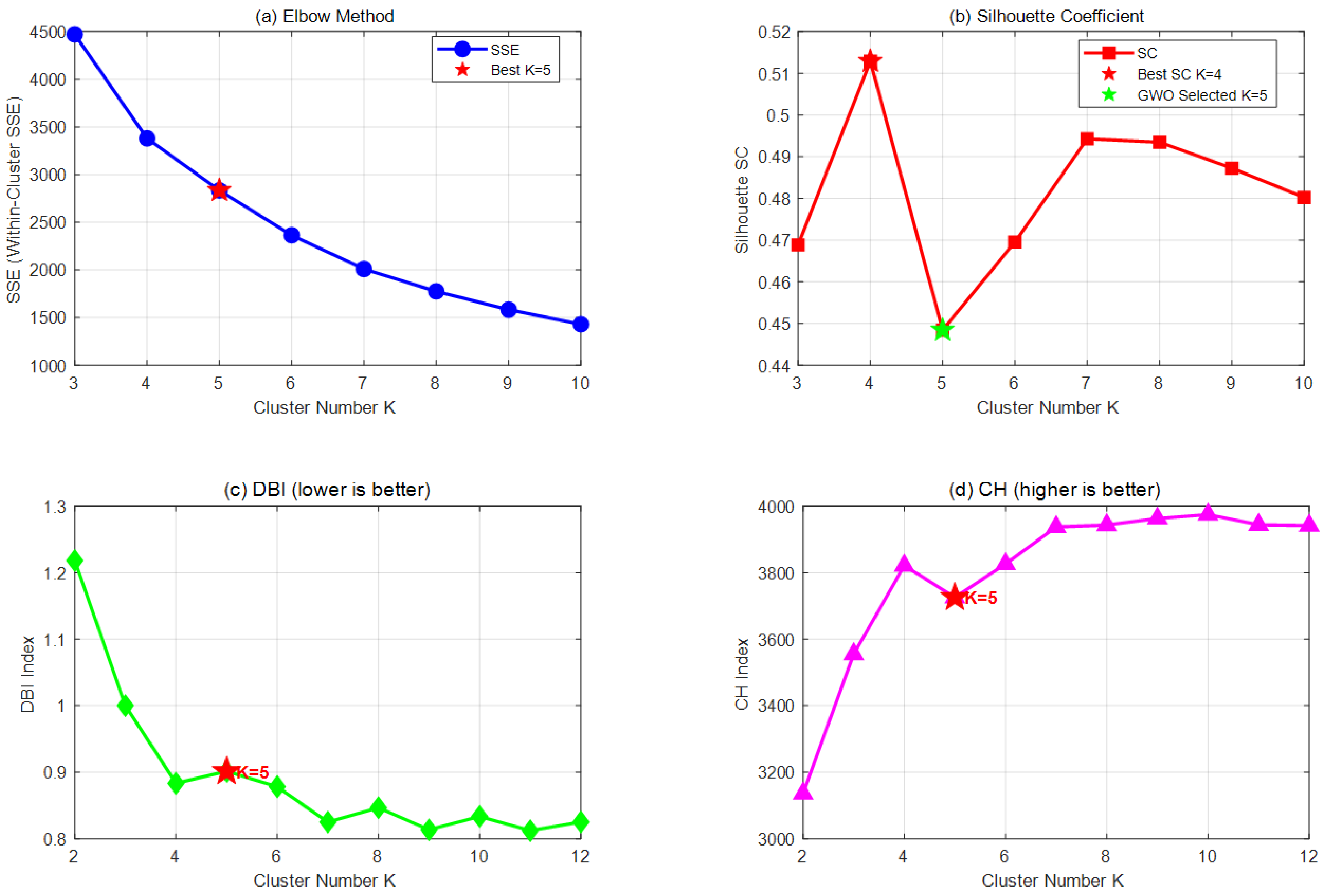
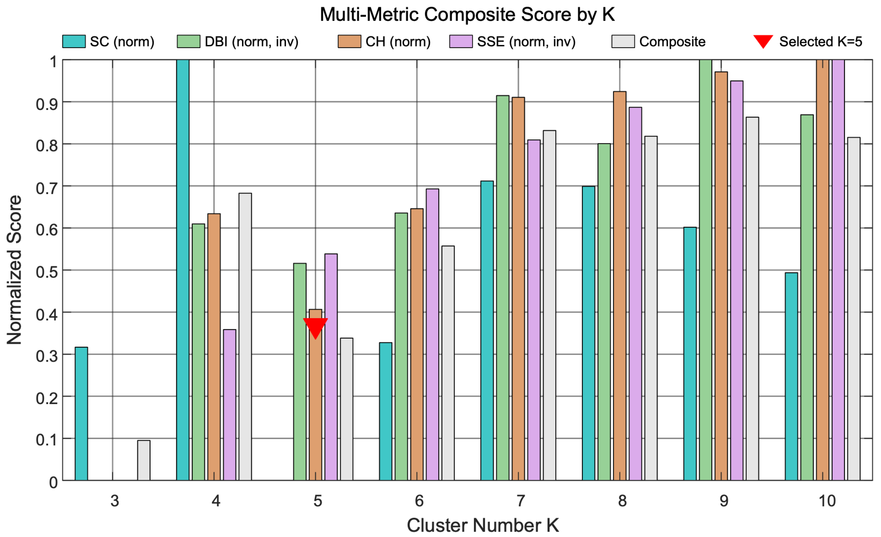
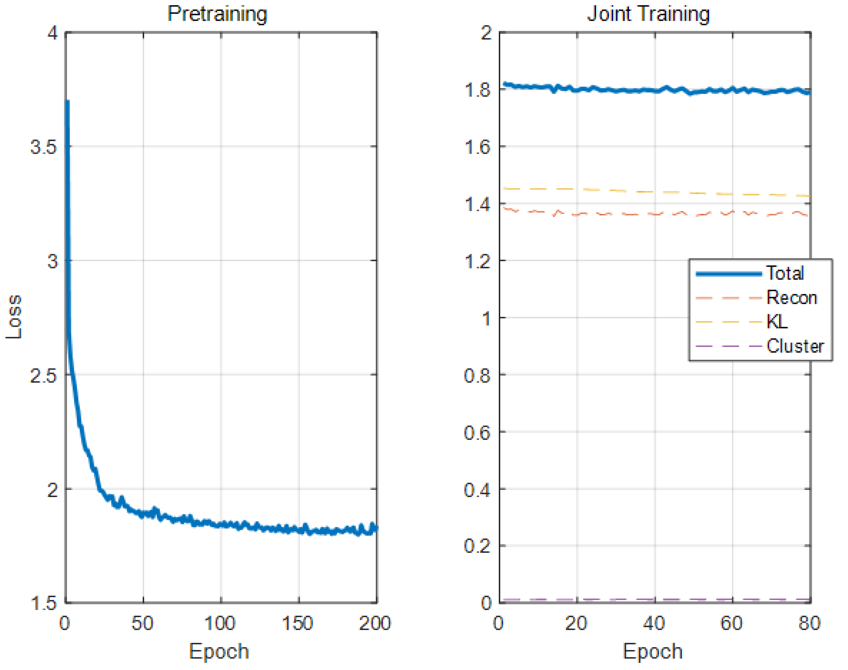
For the representative seed-42 run, adaptive GWO selected K = 5. Supplementary Figure S2 separates the loss components so that the clustering loss can be inspected on its own scale, and Supplementary Figure S3 reports the retained global-best GWO fitness and its associated K trajectory. These optimization curves describe the representative run and are not a substitute for the repeated-run results. The training loss curves are shown in Figure 5.

The representative pretraining objective decreased and then stabilized. During joint refinement, the reconstruction, KL, and clustering-loss components remained finite. Loss curves describe numerical optimization behavior; they do not independently establish improved clustering quality.

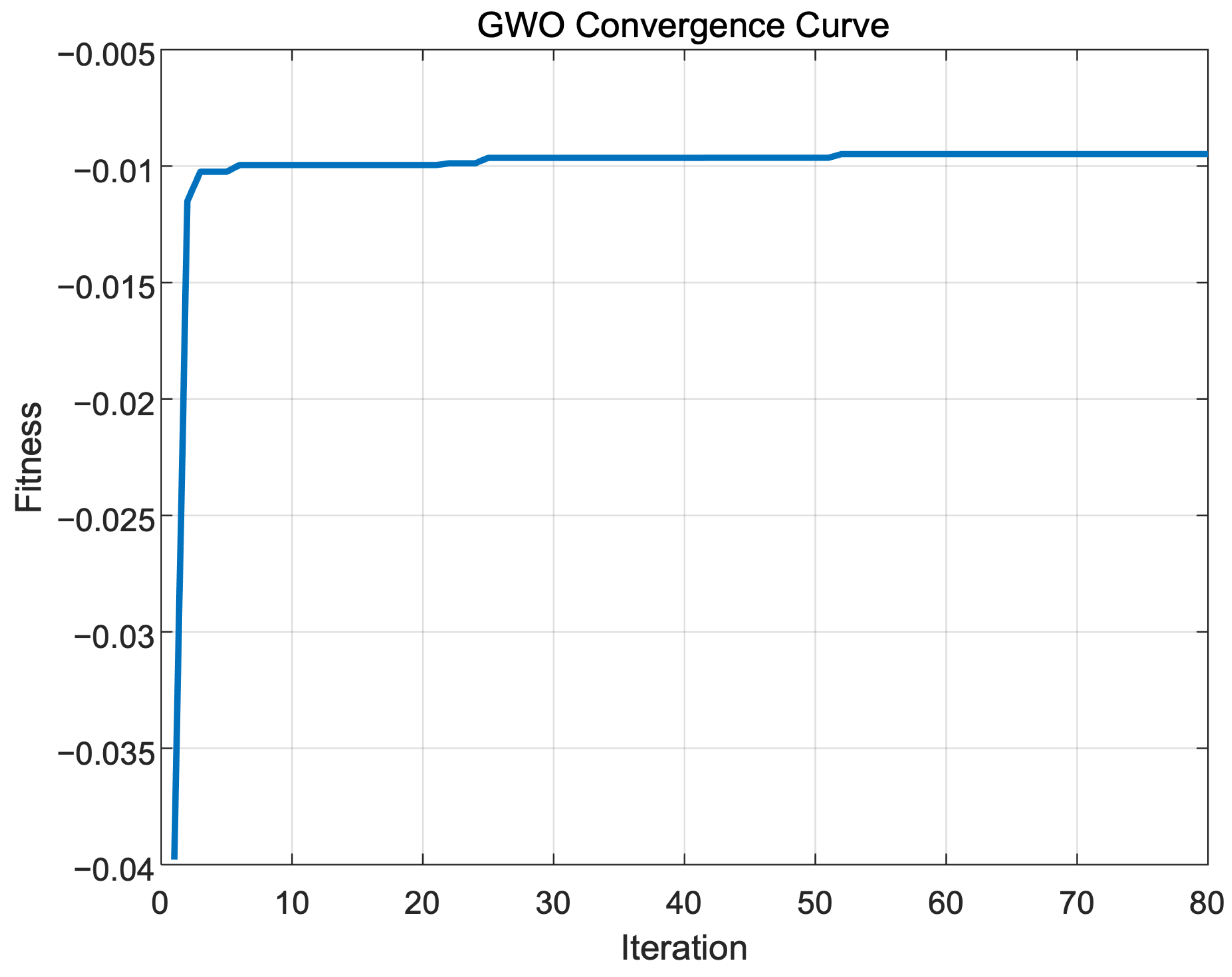
Figure 6 shows the best fitness value observed during GWO optimization. Fitness increases rapidly within the first five iterations and stabilizes after approximately 10 iterations, indicating that the search converges well within the selected 80-iteration budget.

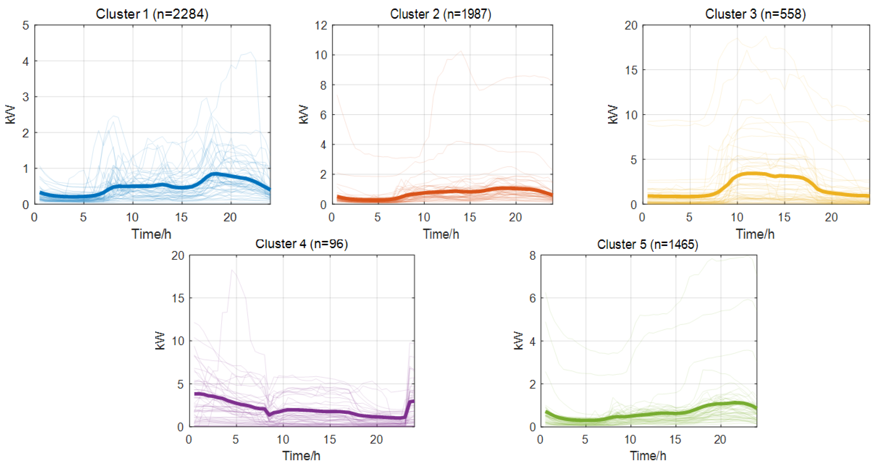
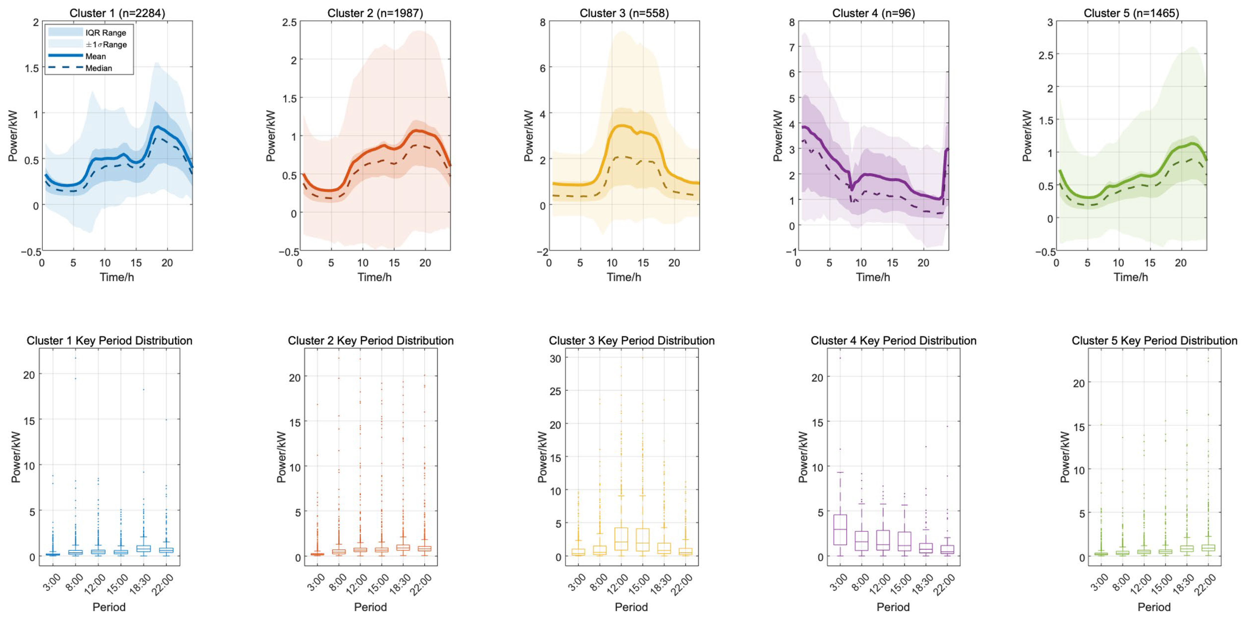
For each cluster, the mean load at every time point is used to construct a representative daily load curve. Boxplots summarize the corresponding distribution across users, including the median, quartiles, and dispersion [17]. Figure 7 presents the representative daily curves, and Figure 8 presents the distributional summaries and mean curves.

Figure 8 further compares the electricity-use distributions of the five clusters. In the upper row, the solid line denotes the mean, the dashed line denotes the median, the dark band denotes the 25–75% interquartile range (IQR), and the light band denotes plus or minus one standard deviation. The lower row presents boxplots at six representative times: 04:00, 08:00, 12:00, 16:00, 20:00, and 24:00.

Cluster 1 maintains low mean and median loads throughout the day and has a narrow IQR, indicating consistent low-load behavior. Cluster 2 has a similar curve shape but slightly higher afternoon and evening demand and a wider IQR. Clusters 1 and 2 therefore show relatively concentrated and regular electricity use. Cluster 3 exhibits high daytime demand and a wider distribution, reflecting greater variation in consumption and peak magnitude. Cluster 4 has high nighttime and early-morning loads that subsequently decline, a pattern that may correspond to thermal-storage heating or other nighttime operation. Cluster 5 remains low in the morning and rises gradually from afternoon to evening.

The boxplots are consistent with the patterns identified from the mean curves. Model training and clustering use normalized load curves; for engineering interpretation, Figure 7 and Figure 8 show inverse-normalized curves and boxplots in the original load units.

6.2. Residential Load Profiles and User-Profile Interpretation

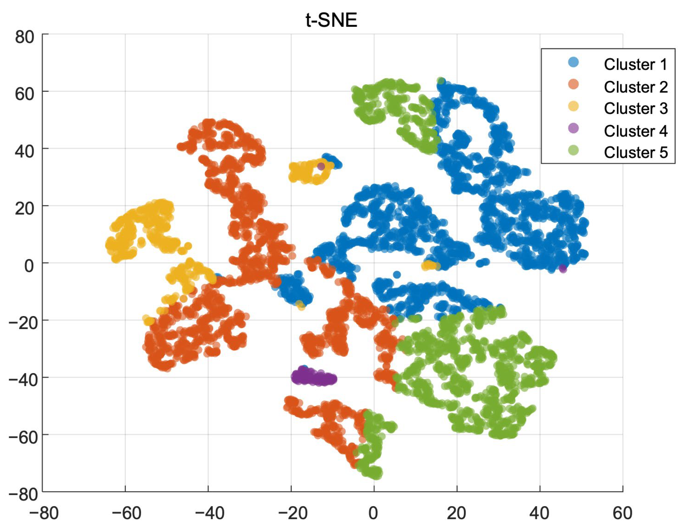
For qualitative visualization [24], t-SNE projects the 16-dimensional latent representations from the representative seed-42 K = 5 run into two dimensions (Figure 9). The display uses fixed settings and illustrates the selected partition only; it is not used as quantitative evidence of cluster stability or global separation.

The t-SNE visualization in Figure 9 shows distinct structure among the learned representations. Clusters 3 and 4 occupy relatively isolated regions, consistent with their distinctive electricity-use patterns. Clusters 1 and 5 each form several dense subgroups with visible separation, while limited overlap occurs near the boundaries of Clusters 1, 2, and 5, whose load shapes are similar but differ in peak timing and load level.

Overall, the visualization shows greater proximity among users assigned to the same cluster than among users assigned to different clusters. This pattern supports the ability of CA-VAE latent features to represent differences in residential electricity use, while limited overlap remains among clusters with similar load shapes.

For each cluster, peak time, load factor (mean/peak), and peak-to-valley difference ratio ((peak-valley)/peak) are calculated. These indicators are combined with daily load-curve shape to define the user-profile labels reported in

Table 1. User-profile labels.

Cluster	Profile	Users	Peak (h)	Load Factor	P-V Ratio	Shape	Feature
C1	Low-load evening peak	2284	18.5	0.57	0.76	Narrow peak	Short evening use
C2	Medium-low broad peak	1987	18.5	0.66	0.74	Broad peak	Sustained use
C3	High-load daytime peak	558	11.5	0.54	0.75	Day peak	Daytime use
C4	High-load nighttime peak	96	1.0	0.54	0.74	Night peak	Night use
C5	Evening-rising load	1465	21.5	0.58	0.73	Gradual rise	Late-return use

.

The five profiles differ in peak timing, load level, and curve shape. Cluster 1 is a low-load evening-peak profile; Cluster 2 is a medium-low-load broad evening-peak profile; Cluster 3 is a high-load daytime-peak profile; Cluster 4 is a high-load nighttime profile; and Cluster 5 is an evening-rising profile.

The profiles are interpretable in terms of electricity-use period, load level, and curve shape and therefore imply different load-regulation opportunities [25]. For example, Cluster 3 may respond to a noon peak tariff, Cluster 4 may be suited to valley-period incentives, and Clusters 1 and 5 may support evening peak-shaving programs. These differences can inform fine-grained demand-side management and differentiated tariff design.

6.3. Demand-Response Implications

The five profiles are behavioral user profiles derived from load curves, not observed demand-response actions or validated flexibility resources. Their peak timing, relative valley depth, and shape can be used to formulate candidate profile-specific participation measures for later field evaluation. Any such evaluation requires actual program participation, response events, tariff conditions, and absolute load information.

Table 2. Demand-response potential analysis of each user cluster.

Cluster	Profile	Users	Peak Shave	Valley Fill	Shift	Window	Strategy
C1	Low-load evening peak	2284	Med.	Med.	High	Evening	Shift evening load
C2	Medium-low broad peak	1987	Low	Low	Low	Evening	Routine TOU
C3	High-load daytime peak	558	High	Low	Med.	Noon/day	Peak pricing
C4	High-load nighttime peak	96	Low	High	Low	Night valley	Valley incentives
C5	Evening-rising load	1465	Med.	Med.	Med.-High	Evening/night	Off-peak shifting

summarizes the profile-specific candidate demand-response measures.

(1) Candidate peak-shaving measure. Profiles with daytime or evening peaks may be prioritized for testing targeted price or incentive offers. This inference is based on load-shape characteristics and should not be interpreted as measured response.

(2) Candidate valley-period measure. Profiles with relatively high nighttime or low daytime demand may motivate future tests of valley-period offers, subject to customer acceptance and operational constraints.

(3) Candidate load-shifting measure. Evening-rising or evening-peak shapes may be useful for designing hypotheses about time-of-use offers. Their realized response cannot be inferred from the clustering result alone.

In summary, the profiles can support the formulation of targeted demand-response hypotheses. They should be regarded as candidate groups for future trials rather than as validated operational resources or estimates of dispatchable flexibility.

6.4. Comparative Performance and Ablation Analysis

The revised evaluation compares the final framework with raw K-Means, CA-VAE + K-Means, CA-VAE + PSO-K-Means, and CA-VAE + GMM. All methods are evaluated in the ten independent runs, and

Table 3. Ten-run clustering comparison (mean (SD)).

Interpretation	CH, Mean (SD)	DBI, Mean (SD)	SC, Mean (SD)	Method
Proposed final method	3694.3 (260.5)	0.8532 (0.0383)	0.5002 (0.0314)	Final CA-VAE + GWO-K-Means
Final method better on all metrics	1147.7 (137.5)	1.6358 (0.0796)	0.2618 (0.0310)	Raw K-Means
No uniform final-method advantage	3720.9 (227.9)	0.8607 (0.0610)	0.5101 (0.0227)	CA-VAE + K-Means
No GWO superiority claim at fixed K	3705.6 (234.2)	0.8329 (0.0365)	0.5201 (0.0186)	CA-VAE + PSO-K-Means
Final method better on all metrics	1590.0 (270.2)	1.3544 (0.3103)	0.3279 (0.0439)	CA-VAE + GMM

reports mean and SD. The non-GWO baselines use fixed K = 5 for comparability, whereas the adaptive GWO workflow retains the K selected in each run. PSO uses the same latent features, population size, iteration budget, fitness definition, and local refinement budget as the fixed-K comparison.

(1) K-Means, applied directly to the normalized 48-dimensional data; (2) VAE-K-Means, which uses a conventional fully connected VAE without convolution or attention before K-Means clustering; and (3) VAE-GMM, which applies a Gaussian mixture model to features extracted by a conventional VAE. SC, DBI, and CH are used for evaluation. The non-GWO baselines use fixed K = 5, whereas adaptive GWO retains the K selected in each run; Table 3 reports the results.

Across ten paired runs, the final framework outperformed raw K-Means and CA-VAE + GMM on SC, DBI, and CH (exact paired Wilcoxon p = 0.001953 for each of these metric comparisons). It did not show a uniform internal-metric advantage over CA-VAE + K-Means, CA-VAE + PSO-K-Means, or the pre-joint GWO solution. These outcomes bound the performance claim to the comparisons supported by the data.

Table 4. Ablation and robustness checks.

Interpretation	CH	DBI	SC	Ablation or Check
Joint stage has mixed outcome	3688.8 (223.5)	0.8222 (0.0187)	0.5262 (0.0125)	CA-VAE + GWO-K-Means, pre-joint (10 runs)
Repeated comparator; full results in Table 3	1590.0 (270.2)	1.3544 (0.3103)	0.3279 (0.0439)	CA-VAE + GMM (10 runs)
K = 4; no uniform CH conclusion	3735.6	0.9816	0.4473	Attention off (seed 42)
K = 5 retained in both checks	3393.3; 3459.0	0.8616; 0.8409	0.5219; 0.5353	Gamma = 0.05; fitness weights 0.3/0.7 to 0.7/0.3 (seed 42)

summarizes the ablation and robustness checks. The attention and gamma checks are single-seed analyses and are labeled as such; the repeated-run pre-joint comparison is reported separately to avoid treating a representative run as a statistical conclusion.

The attention-free representative run selected K = 4 and had lower SC and higher DBI than the attention-enabled run, whereas CH was higher under the different K. The gamma sensitivity check retained K = 5 and showed small metric differences. In the ten-run comparison, joint refinement did not provide a uniform gain over the pre-joint GWO solution. We therefore describe attention and joint refinement as assessed components rather than universally beneficial modules.

The ten-run comparison does not support a blanket superiority claim for GWO over every alternative. GWO is retained because it searches K and initial centers jointly; its value is therefore assessed through the reported modal K = 5 solution, the controlled robustness checks, and the bounded comparisons in Table 3.

In the ten-run comparison, the pre-joint GWO solution had higher mean SC and lower mean DBI than the final joint-refined solution, while the final solution had a slightly higher mean CH (3694.3 versus 3688.8). The clustering-loss stage is consequently reported as a tested refinement rather than as a uniformly improving step.

The original PCA-K-Means statement is not retained as a central comparative claim in this revision. The repeated-run comparison instead reports raw K-Means, CA-VAE + K-Means, CA-VAE + PSO-K-Means, and CA-VAE + GMM, for which the scope of supported conclusions is stated in Table 3.

Overall, the repeated-run results support a limited conclusion: the final workflow is clearly better than raw K-Means and CA-VAE + GMM on the reported internal metrics, while comparisons with CA-VAE + K-Means, CA-VAE + PSO-K-Means, and the pre-joint GWO solution are mixed. The method contribution is the integrated and reproducibly evaluated workflow, not a claim of universal dominance by each component.

6.5. Limitations and Future Research

The present evidence has five important limitations. First, the framework is evaluated only on prepared CER average-day profiles, and external generalizability is not established. Second, aggregation suppresses day-level, seasonal, and weekday–weekend variation. Third, raw daily data were not available to re-evaluate imputation or outlier handling. Fourth, the repeated-run analysis indicates that profile stability varies, particularly for a small day-load profile. Fifth, demand-response implications are inferred from load shape rather than observed response events. The profiles should therefore be used for program screening and hypothesis design, not as direct estimates of dispatchable flexibility.

Future work should validate preprocessing alternatives on raw daily records, test the workflow on independent regional datasets and rolling time windows, assess scalability under larger deployments, and combine profile assignments with observed demand-response events. These steps are required before claims about operational flexibility or cross-region transferability can be made.

7. Conclusions

This study evaluates a residential user-profiling framework that combines CA-VAE representation learning, adaptive GWO-K-Means search, and clustering-loss refinement. The CER evidence supports the following bounded conclusions:

(1) The final framework outperformed raw K-Means and CA-VAE + GMM on the three internal clustering metrics across ten paired runs.

(2) GWO searched K and initial centers in the latent space. K = 5 was the modal result (6/10 runs) and was retained as the representative, interpretable solution rather than a unique optimum.

(3) Attention and clustering-loss refinement were assessed with bounded ablations. They did not establish a uniform improvement across all internal metrics, so the corresponding claims are limited accordingly.

(4) The resulting profiles provide load-shape-derived candidate groups for future demand-response design. They do not validate customer response, aggregate flexibility, or transferability beyond the CER setting.