Neural Network-Based Real-Time Wind Energy Estimation

Abstract

This work proposes a real-time wind power estimation approach for a direct-current (DC) wind energy conversion system based on an artificial neural network (ANN). The proposed ANN uses the Levenberg–Marquardt (LM) algorithm and is trained using experimental data collected from a LabVolt wind energy test bench. The objective is to accurately estimate the instantaneous electrical power generated from the measured wind speed under different operating conditions. The proposed methodology comprises experimental data acquisition, ANN training, algorithm comparison, and model validation. The training performance of the LM algorithm was compared with that of the Resilient Backpropagation algorithm using the same dataset and network architecture. The results demonstrate that the LM algorithm provides superior convergence and prediction accuracy for the considered dataset. The selected ANN model achieved an MSE of 0.240601, an RMSE of 0.490511, an MAE of 0.207092, and a coefficient of determination of (R² = 0.999964). These results demonstrate an excellent agreement between the measured and predicted power values. The proposed ANN-based approach provides an accurate and computationally efficient solution for real-time wind power estimation and shows strong potential for integration into intelligent energy management systems and digital twin frameworks for wind energy conversion systems.

1. Introduction

The energy transition has been identified as a pivotal strategy for mitigating the effects of climate change. A range of targeted measures has been proposed as means of reducing carbon emissions from electricity generation, including enhancing process efficiency and developing renewable energy sources [1,2]. In the realm of renewable energy sources, wind power occupies a pivotal position, primarily due to its minimal environmental impact and considerable energy potential [3]. The development of isolated electrical systems has been identified as a significant solution to promote their utilization and enhance the profitability of industrial production [4]. Nonetheless, the intermittent nature of wind power, in conjunction with its high degree of non-linearity, renders its forecasting particularly complex, particularly in the context of small installations integrated into microgrids [5,6]. In this context, real-time estimation of production represents a significant challenge in terms of enhancing control quality, optimizing energy management, and ensuring system stability [7].

Owing to its highly non-linear nature and the associated uncertainties pertaining to wind variations, the generation of wind power remains a challenging endeavor to predict using conventional approaches [8]. In this context, artificial intelligence approaches—and more specifically, artificial neural networks—open new possibilities thanks to their ability to model complex, non-linear relationships derived from experimental data.

A substantial amount of research has been conducted on the utilization of machine learning and artificial intelligence algorithms for the real-time monitoring of energy production to provide precise estimations. Several multi-objective predictive models were developed using various advanced machine learning (ML) techniques, including artificial neural networks (ANNs), recurrent neural networks (RNNs), convolutional neural networks (CNNs), and long short-term memory (LSTM) networks [9]. As posited by reference [10], the utilization of physics-inspired deep neural networks (DNNs) is advocated for the real-time monitoring of electrical systems. This approach is purported to enhance system comprehension, encompassing anticipatory capabilities across the designated time horizon, while concomitantly augmenting the resilience of the DNN-based estimator. In [11], an approach based on artificial neural networks (ANNs) is proposed for the short-term forecasting of wind turbine power, utilizing swarm intelligence algorithms. Three distinct methodologies are implemented for the effective processing of data. Firstly, there is a conventional artificial neural network (ANN). Secondly, there is an ANN that has been optimized by the firefly algorithm (ANN-FA). Thirdly, there is an ANN that has been optimized by the particle swarm optimization algorithm (ANN-PSO). As outlined in [11], a plethora of architectures for enhancing neural networks have been proposed in the extant literature. Many studies demonstrate that the Backpropagation algorithm is an effective supervised learning method for training artificial neural network (ANN) models and establishing a functional relationship between continuous input and output variables.

As demonstrated in reference [12], the proposed artificial neural network (ANN) has been shown to optimize the operation of the hybrid system by providing an effective estimate of wind and solar energy production for a given set of weather conditions. The Levenberg–Marquardt training algorithm was selected based on its rapid convergence and effective minimization of the mean square error. This makes it especially well-suited to small- and medium-sized networks employed in energy prediction applications. Nevertheless, as the work is founded on a particular dataset, the extent of the conclusions remains constrained. Moreover, the heterogeneity of wind turbine designs acts as a limiting factor for the generalization of the results.

The originality of this work lies in the application of an ANN-based wind power prediction approach to a DC wind energy conversion system using real experimental data, together with comprehensive experimental validation. The conversion of kinetic energy into electrical energy is a nonlinear process involving the power coefficient Cp, mechanical losses in the shaft, and the efficiency of the generator–converter system. The proposed artificial neural network (ANN) overcomes this physical complexity by directly learning the relationship between wind speed and power from data measured on the LabVolt test bench. The network is trained using the Levenberg–Marquardt algorithm, chosen for its rapid convergence and accuracy on nonlinear regression problems.

Section 2 is devoted to modeling the wind power generation system and presents an overview of the system under study. Section 3 then develops the energy forecasting model based on an artificial neural network. Finally, Section 4 presents the results and discussion.

2. Wind Power Generation

2.1. System Under Investigation

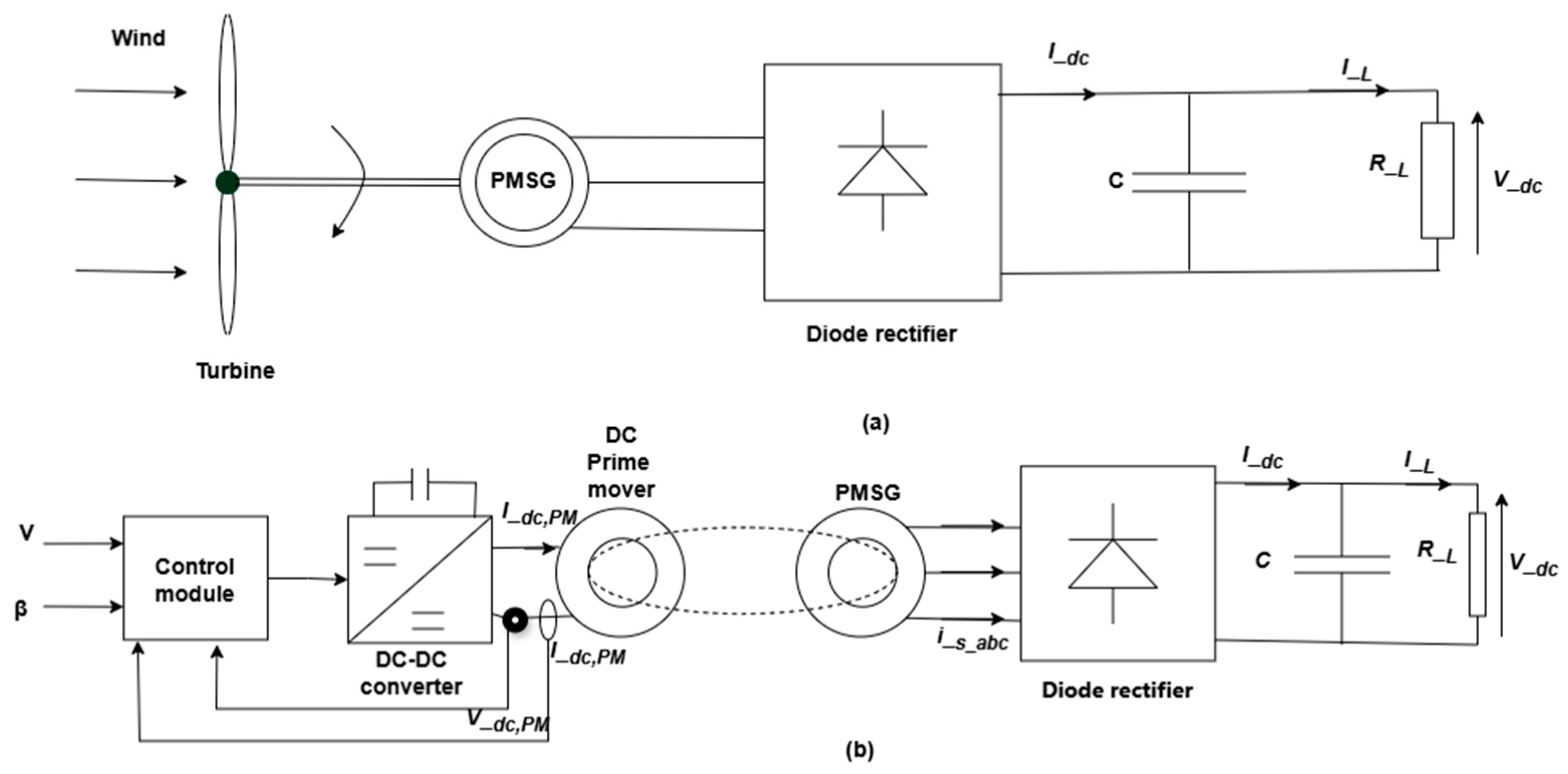
As illustrated in Figure 1a, the wind power system under investigation comprises a variable-speed wind turbine directly coupled to a permanent magnet synchronous generator (PMSG). The mechanical energy extracted from the wind by the turbine is converted into electrical energy by the generator, which is then fed to a diode rectifier, thereby converting the alternating current produced into direct current. Figure 1b illustrates the equivalence of the wind power system implemented on the LabVolt test bench using the wind power emulator. The module employed is the LabVolt Series 8216-01 (Festo Didactic Inc., Québec, QC, Canada), dedicated to the alternator and wind turbine controller. This wind turbine generator–controller replicates the operation of a real low-power wind turbine, integrating both the generator and its controller within a full-size EMS module. The module also incorporates auxiliary components, notably a three-phase diode rectifier and a set of three power resistors, allowing a variable electrical load to be applied to the generator. Access to the generator windings, controller inputs and outputs, and the diode rectifier and power resistors is facilitated by color-coded 4 mm safety sockets located on the front panel of the module.

2.2. Mechanical and Electrical Equations

The mechanical energy extracted by the wind turbine from the kinetic energy of the wind can be expressed by Equation (1) [13,14].

$$P_{wind}={\displaystyle \frac{1}{2}}\rho .S.V^3$$

(1)

where:

$P_{wind}$: Kinetic power of the wind in watts (W).

$\rho$: Air density in kg/m³.

V: Wind speed in m/s.

S: Swept area of the turbine blades (m²).

$$S=\pi .R^2$$

(2)

The useful mechanical power extracted from the wind is determined by the turbine power coefficient, C_p, according to the following expression:

$$P_m={\displaystyle \frac{1}{2}}{C}_p\times \rho \times S\times V^3$$

(3)

where:

$P_m$: Mechanical power produced by the turbine (W).

$C_p$: Power coefficient (aerodynamic efficiency).

$0<C_p<0.593$: Betz limit.

In our study, only the generator-related friction coefficient is taken into account. The mechanical behavior of the turbine–generator assembly is described by the following differential equation:

$$T_{wind}=J_t{\displaystyle \frac{d\Omega }{dt}}+T_{em}+f_m\Omega$$

(4)

where:

$J_t$: Turbine inertia in kg.m².

$f_m$: Machine friction coefficient in N.m.s/rad.

$T_{wind}$: Static torque provided by the wind turbine in N.m.

$T_{em}$: Electromagnetic torque of the generator in N.m.

Due to its many advantages over other electric machines, particularly in terms of performance and robustness, the permanent magnet synchronous machine is a particularly suitable solution for use as a generator coupled to a wind turbine [15,16,17].

The equations of the PMSG expressed in the Park reference frame are presented in Equations (5)–(8). These equations describe the electrical behavior of the machine along the (d)- and (q)-axes. The resistive terms represent the voltage drops across the stator resistance, while the inductive terms account for the variation in the stator flux linkages. The speed-dependent term (ωψ) represents the back electromotive force (back-EMF) induced by the rotor magnetic flux and is directly related to the electrical angular speed of the machine:

$$V_d=R_s.i_d+L_s{\displaystyle \frac{d{i}_d}{dt}}-\omega L_s{i}_q$$

(5)

$$V_q=R_s.i_q+L_s{\displaystyle \frac{d{i}_q}{dt}}+\omega L_s{i}_d+\omega \phi$$

(6)

$$\omega =p.\Omega$$

(7)

$$T_{em}={\displaystyle \frac{3}{2}}.p.\psi .i_q$$

(8)

where:

$i_d$ and $i_q$ are the stator currents in Park’s coordinate system in amperes (A).

$V_d$and $V_q$ are the stator voltages in Park’s coordinate system in volts (V).

$R_s$ and $L_s$ are, respectively, the stator resistances in ohms (Ω) and the stator cyclic induction in henries (H).

$\psi$ and $p$ are, respectively, the permanent magnet flux linkage (Wb) and the number of pole pairs.

$T_{em}$ is the electromagnetic torque in N.m.

3. Artificial Neural Network-Based Energy Prediction Model

The accurate prediction of the power output of a wind turbine system is imperative for optimizing its operation, effective energy utilization planning, and enhancing grid stability. However, the inherently variable nature of wind and the intricate dynamics of electrical machines pose significant challenges in this endeavor. To address this challenge, various fundamental artificial neural network (ANN) models have been employed to enhance the precision of wind turbine forecasting [9,11,18,19,20]. In this context, the utilization of artificial neural networks (ANNs) constitutes a contemporary, efficacious, and progressively prevalent methodology. The employment of artificial neural networks (ANNs) is unequivocally endorsed for the estimation of the power output of a wind turbine at varying wind speeds, particularly through the implementation of the Levenberg–Marquardt optimization algorithm [21].

3.1. Model Structure

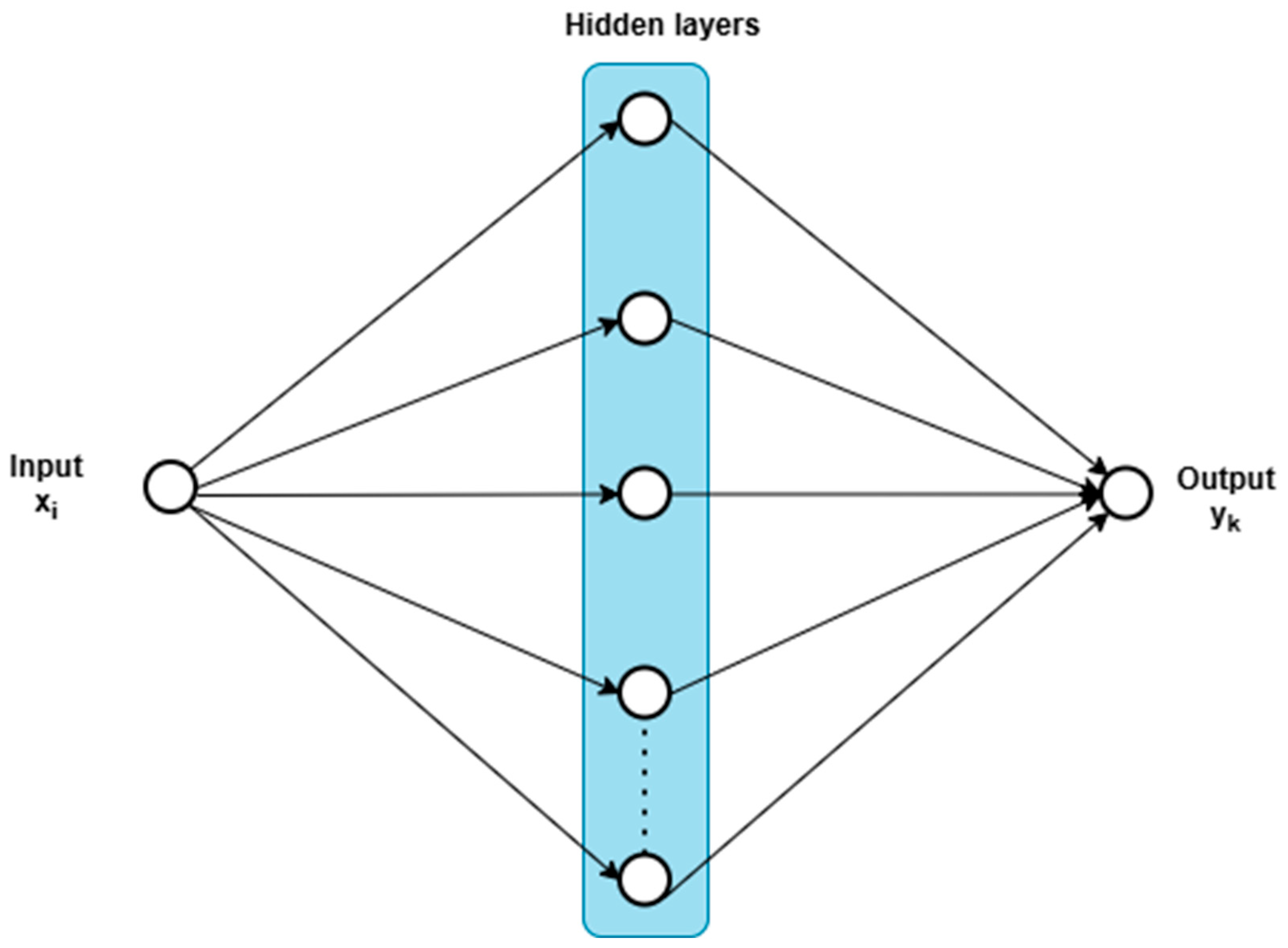
The model is predicated on artificial neural networks (ANNs) and employs the Levenberg–Marquardt (LM) optimization algorithm. It utilizes a feedforward neural network architecture, a type of network that is particularly well suited to regression and prediction problems due to its capacity to approximate complex nonlinear functions. Figure 2 provides a diagrammatic representation of the artificial neural network, consisting of an input layer, a hidden layer, and an output layer. In the proposed model, wind speed is used as the input variable, while the electrical power generated serves as the output variable of the artificial neural network.

3.2. Equations

The artificial neural network used consists of an input layer, a hidden layer with ten neurons, and an output layer. The net input of the jth neuron in the hidden layer is given by the following equation:

$$n_j^1={\displaystyle {\sum }_{i=1}^N}{w_{ji}^{\left(h\right)}x}_i+b_j^{\left(h\right)}$$

(9)

where:

$x_i$: iᵉ input of the network.

$w_{ji}^{\left(h\right)}$: Weight connecting input i to hidden neuron j.

$b_j^{\left(h\right)}$: Bias of hidden neuron j.

N: Total number of inputs.

(h): Index of the hidden layer.

The output of the hidden neuron is then obtained by applying the activation function:

$$h_j=f\left(n_j^{\left(h\right)}\right)$$

(10)

The input from the neurons in the hidden layer to the neuron in the output layer is given by the following formula:

$$n_k^{\left(o\right)}={\displaystyle {\sum }_{j=1}^{10}}{w_{kj}^{\left(o\right)}h}_j+b_k^{\left(o\right)}$$

(11)

where:

$h_j:$Output of the jᵉ neuron in the hidden layer.

$w_{kj}^{\left(o\right)}$: Weight connecting hidden neuron j to output neuron k.

$b_k^{\left(o\right)}$: Bias of the output neuron.

(o): Index of the output layer.

The output layer y_k represents the output of the neural network under study and is given by the following formula:

$$y_k=f^{\left(o\right)}\left(n_k^{\left(o\right)}\right)$$

(12)

where:

$f^{\left(o\right)}$ is the activation function of the neuron in the output layer, which is purely linear and can be written as follows:

$$f^{\left(o\right)}\left(n\right)=purelin\left(n\right)=n$$

(13)

In order to verify the performance of this prediction method, the mean square error (MSE), root mean square error (RMSE) and mean absolute error (MAE) are used as performance indicators. They are defined by the following equations:

$$MSE={\displaystyle \frac{1}{m}}{\displaystyle {\sum }_{i=1}^m}{\left(y_i^{ref}-y_i\right)}^2$$

(14)

$$RMSE=\sqrt{{\displaystyle \frac{1}{m}}{\displaystyle {\sum }_{i=1}^m}{\left(y_i^{ref}-y_i\right)}^2}$$

(15)

$$MAE={\displaystyle \frac{1}{m}}{\displaystyle {\sum }_{i=1}^m}\left|y_i^{ref}-y_i\right|$$

(16)

where:

m: Total number of samples.

$y_i^{ref}$: Reference value.

$y_i$: Value predicted by the neural network.

${\overline{y}}^{ref}$: Mean value of the measured (reference) power.

The coefficient of determination R² is a statistical indicator used to evaluate the quality of fit of a prediction model. It measures the proportion of the variance in the reference variable explained by the model.

$$R^2=1-{\displaystyle \frac{\frac{1}{m}{\displaystyle {\sum }_{i=1}^m}{(y_i^{ref}-y_i)}^2}{\frac{1}{m}{\displaystyle {\sum }_{i=1}^m}{(y_i^{ref}-{\overline{y}}^{ref})}^2}}$$

(17)

4. Results and Discussion

4.1. Experimental Setup

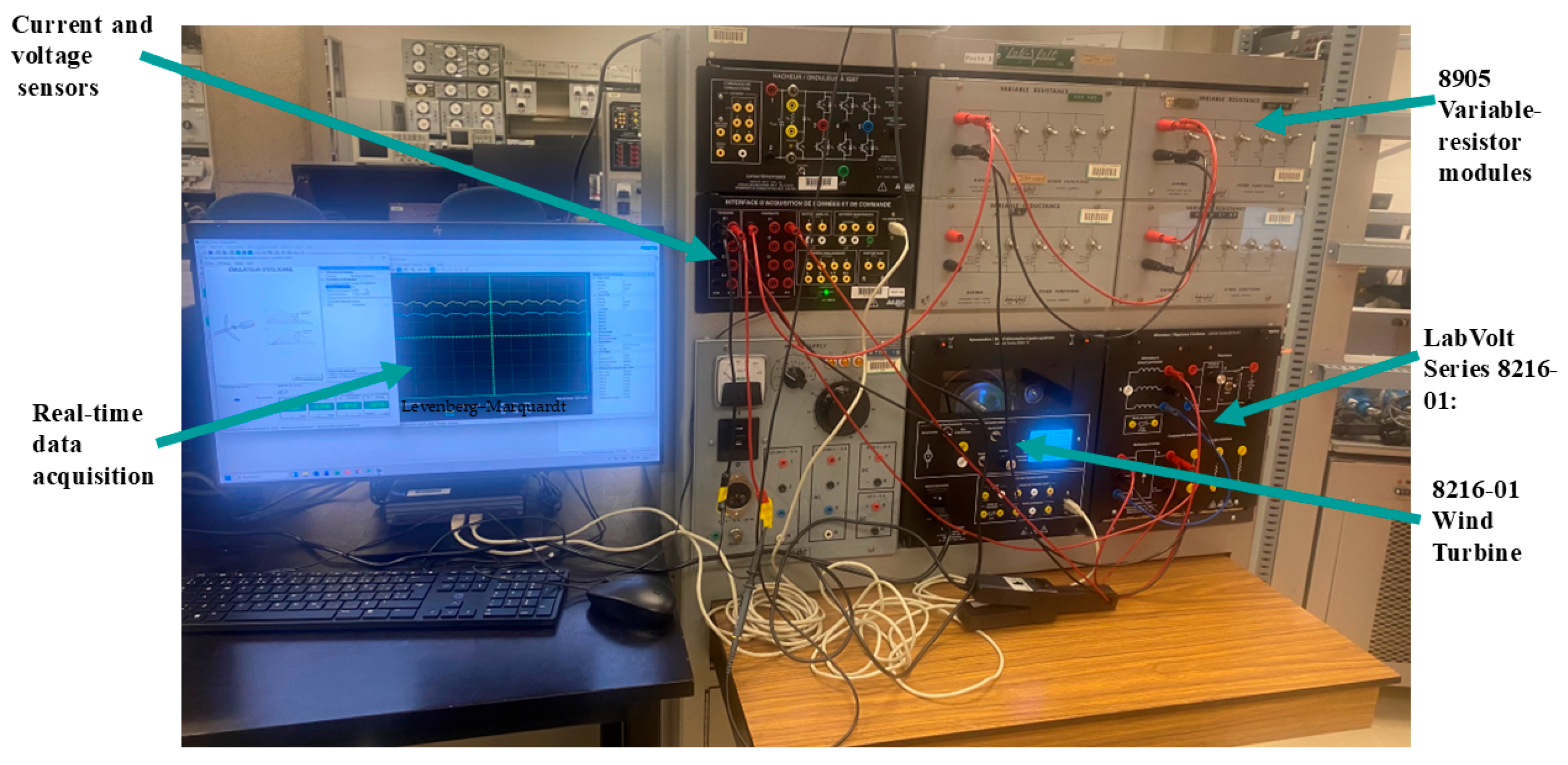
This section presents the experimental setup developed for the study, as well as the various equipment and measuring devices used. The module used was the LabVolt Series 8216-01 Wind Turbine Alternator/Regulator. The system setup diagram is shown in Figure 3. The experimental setup of the wind power system includes a turbine, a three-phase synchronous permanent magnet generator, an uncontrolled diode rectifier, and a resistive electrical load. Using current and voltage sensors, the acquisition system records electrical quantities in real time and then calculates the power.

The experimental platform shown in Figure 3 is based on a LabVolt (Festo) wind turbine emulator. It consists of an 8960-21 Four-Quadrant Dynamometer/Power Supply mechanically coupled to an 8216-01 Wind Turbine Alternator/Regulator module equipped with a six-pole-pair permanent magnet synchronous generator (PMSG). The PMSG is connected to a three-phase six-pulse diode rectifier supplying a 15 Ω resistive load, assembled from two 8905 variable resistor modules and connected in parallel. The experimental measurements were performed at the output of the AC/DC diode rectifier.

The wind speed profile and electrical signals were recorded and stored in MATLAB R2024b compatible format. The acquired data were subsequently transferred to a PC and imported into MATLAB/Simulink for offline processing and analysis. The analog electrical signals were sampled at a frequency of 1000 Hz, resulting in a total of 980 samples. The measured voltage, current, and wind speed data were then processed to characterize the electrical power delivered by the wind turbine emulator and to provide the experimental dataset used for ANN development and validation.

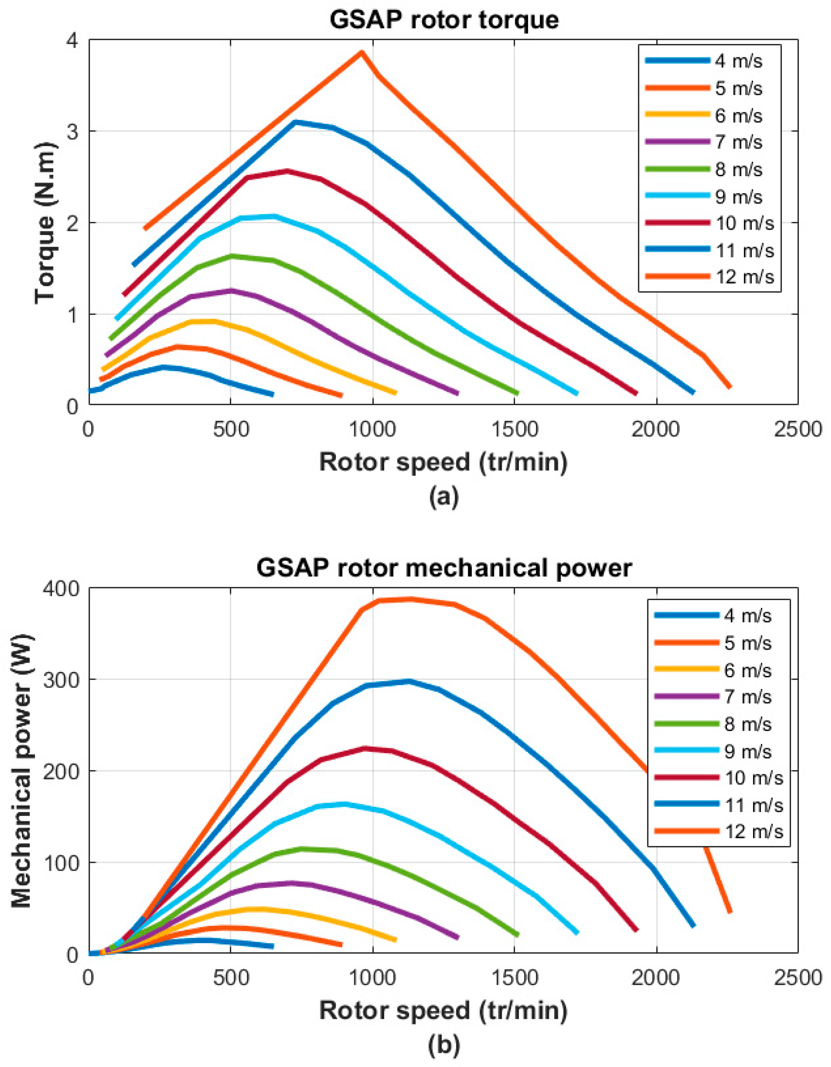
The mechanical power characteristic of the synchronous generator as a function of wind speed, as well as the torque characteristic as a function of rotor rotational speed, was obtained by varying the electrical load from 0 to the maximum allowable load condition and the wind speed from 5 to 12 m/s. In addition, the mechanical power was plotted as a function of wind speed under different load conditions to characterize the generator operating behavior over the investigated operating range.

For the measurements used in the proposed prediction model, the wind speed was varied from 5 to 12 m/s, while the electrical load was maintained at 15 Ω. The measured voltage and current were subsequently used to calculate the electrical power.

The mechanical power characteristic of the synchronous generator rotor as a function of wind speed, as well as the torque characteristic as a function of rotational speed, are shown in Figure 4.

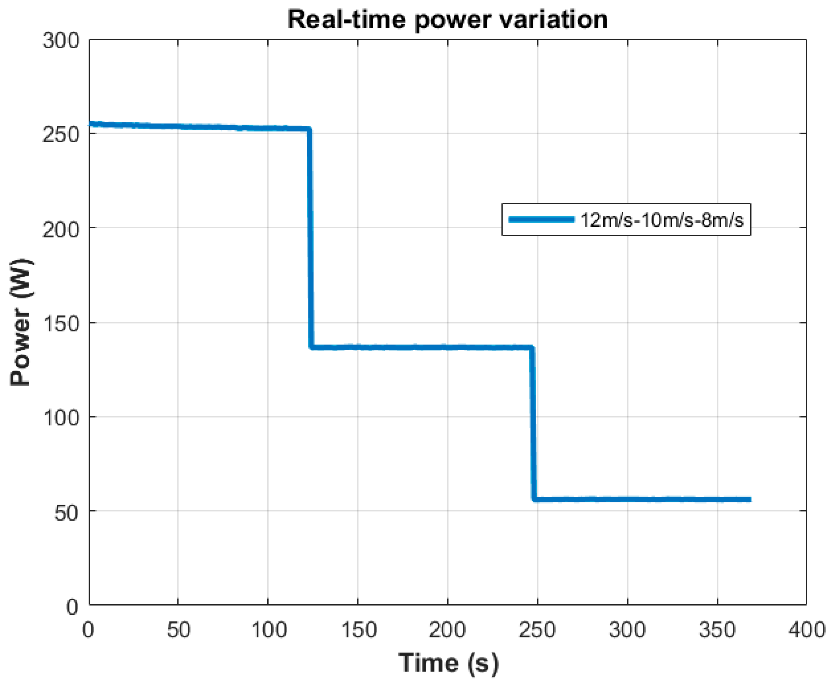
Figure 5 shows the real-time power variation for wind speeds of 12 m/s, 10 m/s, and 8 m/s.

4.2. Prediction Using an Artificial Neural Network

The estimation of wind turbine power from environmental variables measured in real time represents an important challenge for the control and optimization of microgrids. In this context, an artificial neural network (ANN) was implemented to develop a predictive model capable of accurately capturing the nonlinear relationship between wind speed and electrical power output. The objective was to establish reliable mapping between the experimentally measured wind speed and the corresponding electrical power generated by the wind energy conversion system.

The development of the proposed ANN involves two main steps: the selection of an appropriate training algorithm and the determination of an adequate network architecture. First, the training performance and convergence characteristics of the Levenberg–Marquardt (LM) and Resilient Backpropagation algorithms were compared using the same dataset and ANN architecture. The most suitable training algorithm was then selected based on its convergence behavior and prediction accuracy. Subsequently, a sensitivity analysis was performed to determine the appropriate ANN architecture and to evaluate the influence of the number of neurons in the hidden layer on the prediction performance. To ensure reproducibility and prevent data leakage, a fixed random seed was used for data partitioning, with 20% of the samples randomly reserved as an independent test set prior to ANN training; these test samples were not used during the training or optimization process.

4.3. Comparison of Learning Performance and Convergence Between the Levenberg–Marquardt and Resilient Backpropagation Algorithms

The prediction process uses the same ANN mapping for both training algorithms, while the Levenberg–Marquardt (LM) and Resilient Backpropagation (RP) algorithms differ mainly in the procedure used to update the network weights and biases during training. The LM algorithm is an optimization method based on the Gauss–Newton approximation [22]. The update of the network parameters can be expressed as follows:

$$x_{k+1}=x_k-{\left[J^{T}J+\mu I\right]}^{-1}{J}^{T}e$$

(18)

where:

$x:$ Vector containing the network weights and biases.

$J:$ Jacobian matrix of the errors with respect to the network parameters.

$e:$ Error vector.

$\mu :$ Damping parameter.

$I$: Identity matrix.

Resilient Backpropagation primarily uses the sign of the gradient, rather than its magnitude, to determine the direction in which the network weights are updated.

$$x_{ij}^{k+1}=x_{ij}^k-{∆}_{ij}^{k}sign\left({\displaystyle \frac{\partial E}{\partial x_{ij}}}\right)$$

(19)

where:

${∆}_{ij}$ represents the learning step size.

The step size is adjusted according to the change in the sign of the gradient.

Table 1. Performance comparison of the Levenberg–Marquardt and Resilient Backpropagation training algorithms.

Training Algorithms	MSE	RMSE	MAE	(R2)
Levenberg–Marquardt	0.240601	0.490511	0.207092	0.999964
Resilient Backpropagation	1043.42	32.30	27.89	0.84294

compares the performance of the Levenberg–Marquardt and Resilient Backpropagation training algorithms for the proposed ANN.

The results show a clear advantage of the LM algorithm for wind power prediction. Levenberg–Marquardt achieves very low MSE (0.240601), RMSE (0.490511), and MAE (0.207092), together with an R² of 0.999964, indicating an excellent agreement between the predicted and measured power values. In contrast, Resilient Backpropagation produces substantially higher prediction errors, with MSE of 1043.42, RMSE of 32.30, and MAE of 27.89, while its R² decreases to 0.84294. These results indicate that Levenberg–Marquardt provides better convergence and significantly higher prediction accuracy than Resilient Backpropagation for the considered dataset. Therefore, the Levenberg–Marquardt algorithm was selected for the final ANN model.

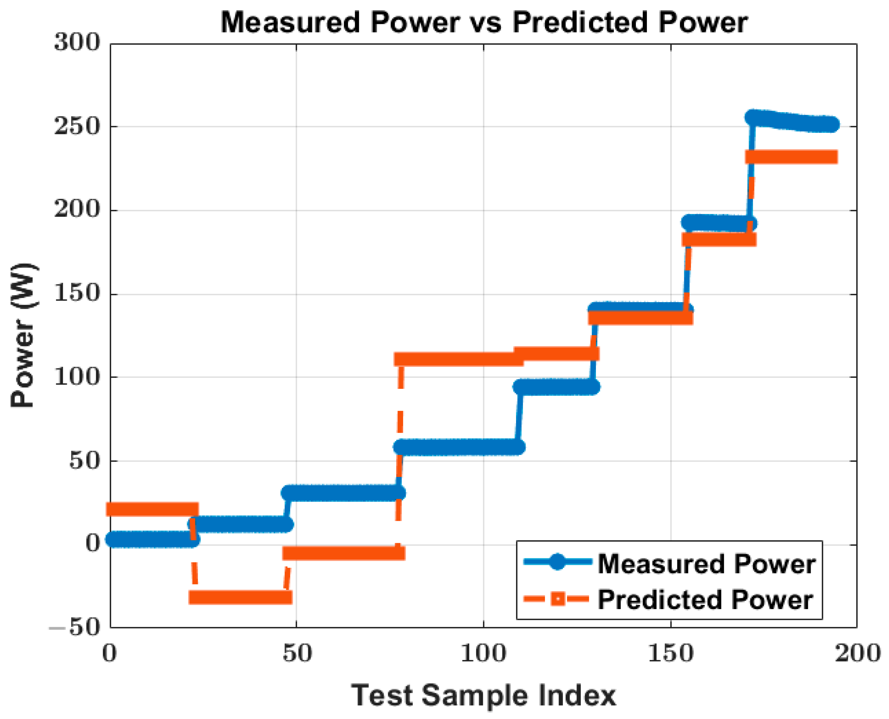
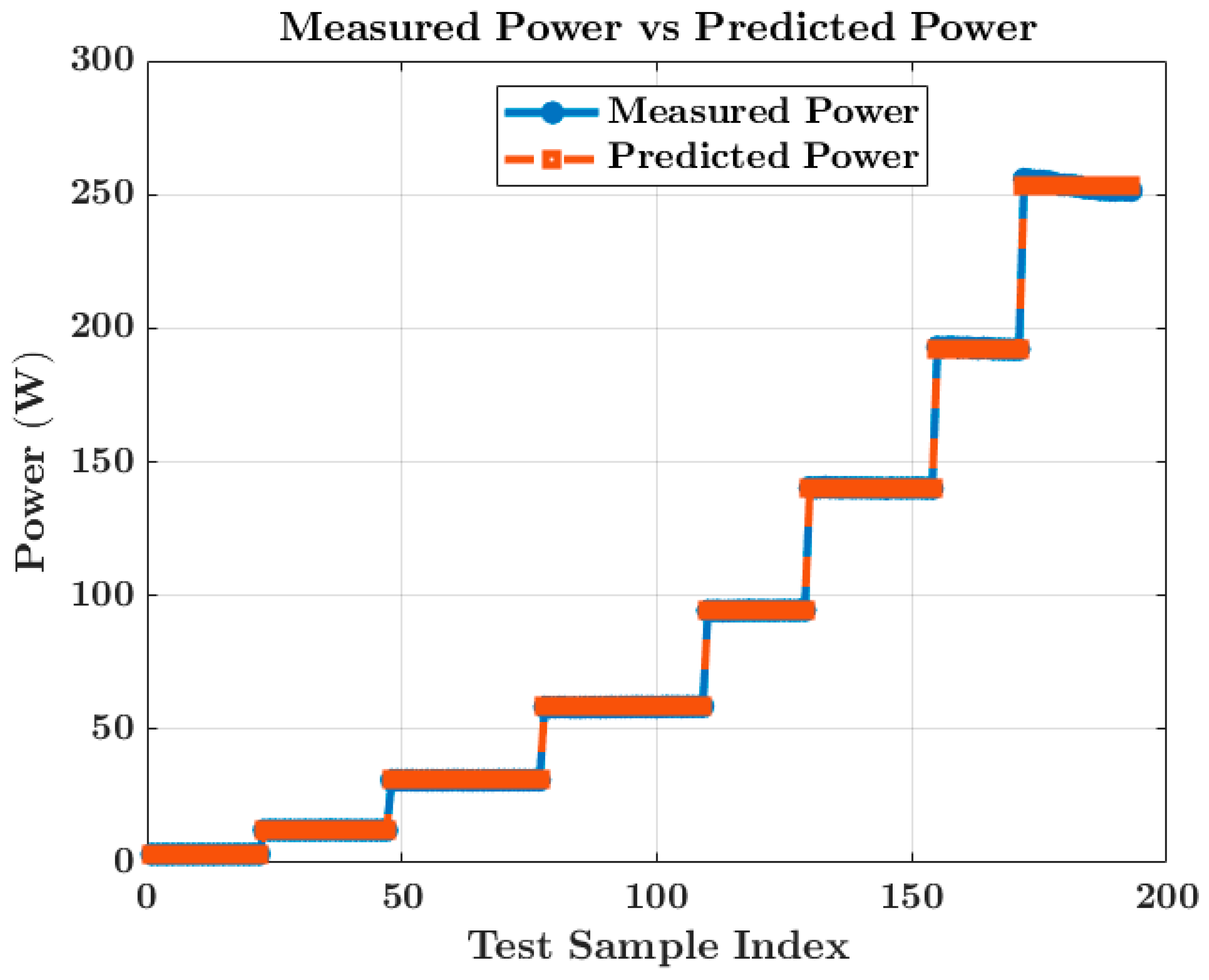
Figure 6 and Figure 7 compare the predictive capabilities of the Levenberg–Marquardt and Resilient Backpropagation algorithms on the same LabVolt dataset. The Levenberg-Marquardt algorithm demonstrates excellent agreement with the measured power, accurately tracking each wind speed plateau from 5 to 12 m/s with negligible error. In contrast, Resilient Backpropagation shows significant deviations, including non-physical negative predictions at 6 m/s and 7 m/s errors exceeding 40 W in the 8–9 m/s range.

4.4. Architecture Selection and Sensitivity Analysis of the Levenberg–Marquardt-Based ANN

The performance of an artificial neural network (ANN) is highly dependent on its architecture, particularly on the number of neurons in the hidden layer. To determine an appropriate network structure while avoiding underfitting and overfitting, a sensitivity analysis was conducted. Three ANN architectures were investigated, comprising 5, 10, and 15 neurons in the hidden layer. All networks employed nonlinear activation functions in the hidden layer and a linear activation function in the output layer. The networks were trained using the Levenberg–Marquardt algorithm, with the dataset divided into training and testing subsets. The performance of each architecture was evaluated using mean squared error (MSE), root mean squared error (RMSE), mean absolute error (MAE), number of training epochs, and coefficient of determination (R²). The results of the sensitivity analysis are presented in

Table 2. Sensitivity analysis of ANN depth.

Number of Neurons Per Hidden Layer	MSE	RMSE	MAE	(R2)
5	0.259371	0.509285	0.225889	0.999963
10	0.240601	0.490511	0.207092	0.999964
15	0.259371	0.509285	0.225889	0.999963

.

The sensitivity analysis evaluates the influence of the number of neurons in the hidden layer on the prediction performance of the proposed neural network. As shown in the table, the 10-neuron architecture provides the best overall performance, achieving the lowest MSE (0.240601), RMSE (0.490511), and MAE (0.207092) values, with an overall value of 0.999964. In comparison, the 5- and 15-neuron configurations produce slightly higher errors, with identical performance values (MSE = 0.259371, RMSE = 0.509285, MAE = 0.225889 and R² = 0.999963). These results indicate that increasing the hidden layer size beyond 10 neurons does not improve the prediction accuracy.

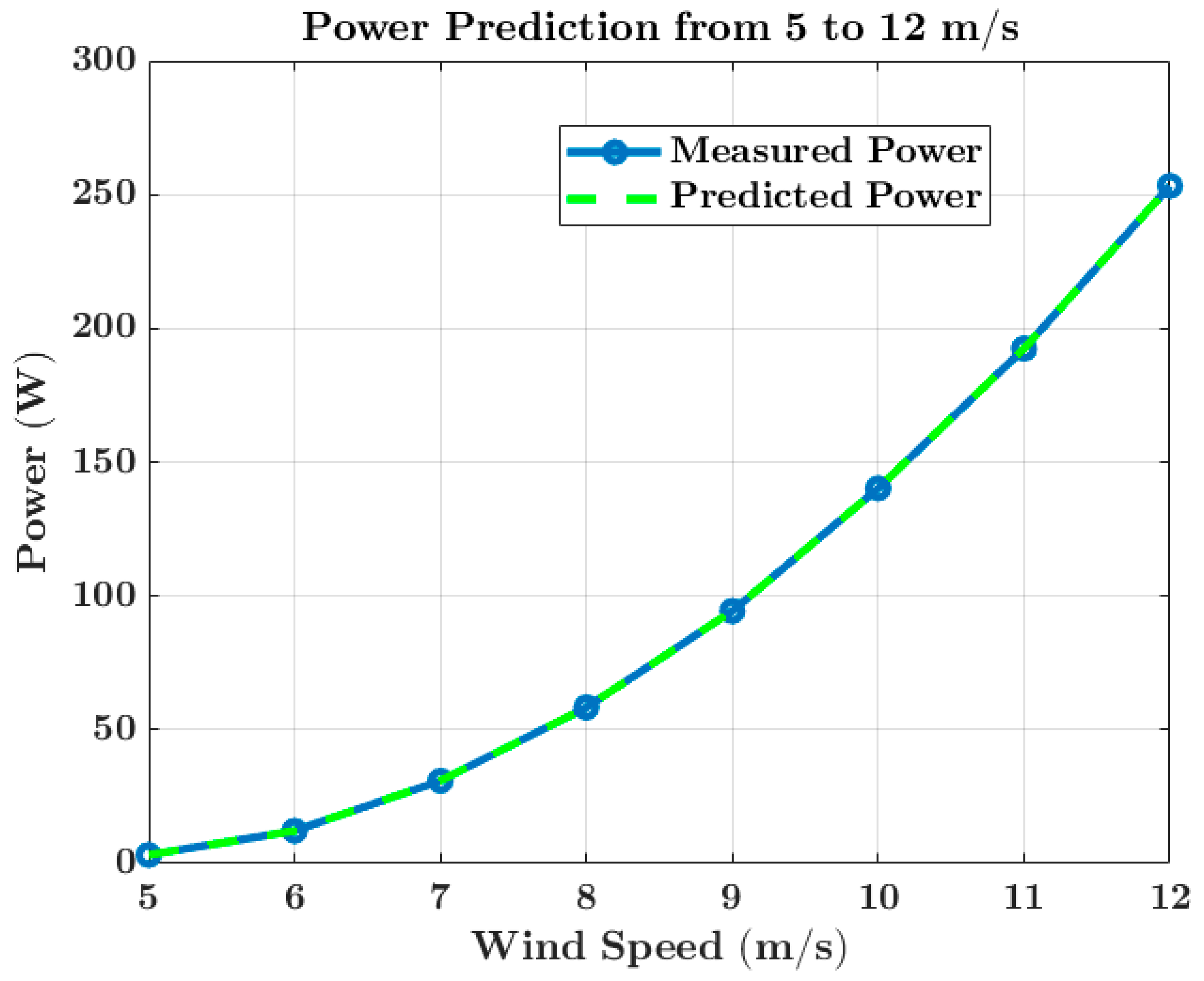
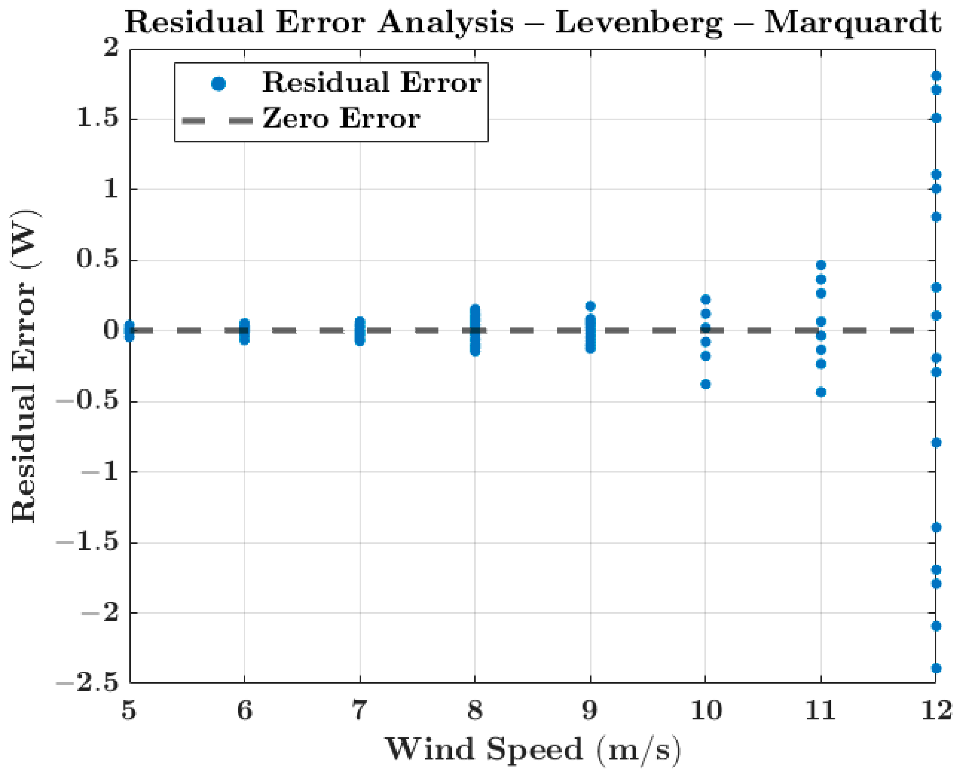
In the following, the same ANN architecture (1-10-1) is used, consisting of one input neuron representing the wind speed, one hidden layer with 10 neurons, and one output neuron corresponding to the predicted wind power. The following figure shows the power prediction for wind speeds ranging from 5 m/s to 12 m/s. Figure 8 illustrates the power prediction for wind speeds ranging from 5 m/s to 12 m/s. The corresponding residual errors versus wind speed are presented in Figure 9, showing error distribution within ±2.5 W across the entire operating range.

4.5. Discussion

The neural network employed, consisting of a single hidden layer with 10 neurons (1-10-1 architecture), provides sufficient capacity to effectively model the nonlinear relationship between wind speed and generated wind power. Figure 8 and Figure 9 illustrate the close agreement between the measured and predicted power values.

The results show an almost perfect overlap between the measured and predicted power curves, indicating that the proposed artificial neural network (ANN) accurately reproduces the system behavior. For each power level corresponding to a given wind speed, the predicted values closely match the measured values, with only minor deviations.

As reported in Table 2, the 1-10-1 architecture demonstrates excellent prediction performance, achieving an MSE of 0.240601, an RMSE of 0.490511 W, and an MAE of 0.207092 W, together with a coefficient of determination of (R² = 0.999964). These results confirm the high accuracy of the proposed ANN in estimating wind power over the investigated operating range.

Figure 9 presents the residual errors, defined as the difference between the measured and predicted power values, as a function of wind speed. For wind speeds ranging from 5 to 11 m/s, the residuals remain tightly distributed around the zero-error line, generally within ±0.5 W, confirming the high prediction accuracy and the absence of significant systematic bias in this operating range. At 12 m/s, a larger dispersion of the residuals is observed, with errors ranging from approximately −2.4 W to +1.8 W. This increased dispersion indicates a degree of heteroscedasticity at the highest investigated wind speed and can be attributed primarily to higher power fluctuations of the LabVolt emulator under maximum-speed operating conditions.

Overall, the results demonstrate that the proposed ANN predicts the generated wind power with high accuracy, showing close agreement between measured and predicted values over the investigated wind speed range of 5–12 m/s. Although the independent test results confirm accurate prediction under the studied operating conditions, the validation remains limited to a single LabVolt experimental platform and the investigated wind speed range. Further validation using unseen wind speeds, different operating conditions, and independent datasets is therefore required to assess the generalization capability of the proposed model. Nevertheless, the ANN demonstrates strong potential for integration into intelligent energy management systems (EMSs) and digital twin frameworks for wind turbine monitoring, power prediction, and predictive energy management.

5. Conclusions

In conclusion, the wind power system investigated in this study is based on a robust architecture consisting of a wind turbine directly coupled to a permanent magnet synchronous generator, followed by a diode rectifier and a resistive load. This configuration enables the accurate reproduction of a typical wind energy conversion chain suitable for microgrid and distributed generation applications.

A series of simulations and experimental measurements were conducted to evaluate the electrical power generated at different wind speeds over the investigated operating range of the turbine. The results demonstrate that the Levenberg–Marquardt algorithm provides faster convergence and higher prediction accuracy than the Resilient Backpropagation algorithm for the considered dataset. Consequently, the Levenberg–Marquardt algorithm was selected for training the final artificial neural network model.

The proposed ANN adopts a 1-10-1 architecture, consisting of one input neuron representing the wind speed, one hidden layer with 10 neurons, and one output neuron corresponding to the predicted wind power. The originality of this work lies in the application of an ANN-based wind power prediction approach to a DC wind energy conversion system using real experimental data, supported by comprehensive experimental validation. The ANN, trained using the Levenberg–Marquardt algorithm, directly learns the nonlinear relationship between wind speed and electrical power from experimental measurements obtained on the LabVolt test bench. The training process exhibited rapid and stable convergence, while the final model achieved a high level of prediction accuracy over the investigated wind speed range. These results demonstrate the potential of the proposed approach for wind power prediction and its future integration into intelligent energy management systems and digital twin frameworks.