Reducing Air Pollution in Rural Areas with Hybrid Heat Pump Supported by Biomass Boiler

Abstract

The widespread deployment of low-carbon technologies in households is increasing the need to reduce peak electricity demand on distribution grids. Air-source heat pumps (ASHPs) are efficient heating units, but their performance declines at low ambient temperatures, increasing winter peak demand. In rural areas, limited grid capacity can constrain their use as a sole heating source, while biomass remains widely used for space heating and contributes to fine particulate matter (PM₁₀) emissions. Unfavourable winter conditions can further increase local pollutant concentrations. This study investigates the potential operating cost savings and PM₁₀ emission reductions when using a biomass-assisted hybrid heat pump (HHP) operating in bivalent mode, while also evaluating GHG emissions relative to a monovalent ASHP, providing a combined assessment not previously applied to biomass-assisted hybrid heat pumps. A validated simulation model was developed to determine the optimal switching temperature using hourly temperature data from 23 locations across Slovenia. The results were interpolated nationally and visualised using GIS tools. The findings indicate that annual cost savings can reach up to 10% and PM₁₀ emission reductions can reach up to 20 kg for a single-family building in colder, mountainous regions.

1. Introduction

According to the Statistical Office of the Republic of Slovenia (SURS) [1], households’ final energy consumption in 2024 was 12,016 GWh, representing 22% of the country’s total final energy consumption. A total of 59% (7032 GWh) of the final energy in households is used for space heating, with biomass being the most widespread source at 49%, followed by extra-light fuel oil at 13%, electricity at 11%, natural gas at 9%, district heat at 9%, and ambient heat at 8%. The share of the latter has been growing steadily since 2012, when it was 1%.

A heat pump is a device that utilises ambient heat with additional work in the form of electricity to satisfy heating demand. Heat pumps can utilise heat from ambient air, water, or the ground. According to the European Commission’s climate target, nearly 60 million heat pumps are expected to be installed in the EU by 2030 [2]. However, air-source heat pumps (ASHPs) exhibit reduced efficiency and thermal output at low outdoor air temperatures, precisely when heating demand peaks. Moreover, real operational data from Central Europe indicate that 17% of ASHPs do not meet existing efficiency standards, and approximately 10% of the systems are oversized [3].

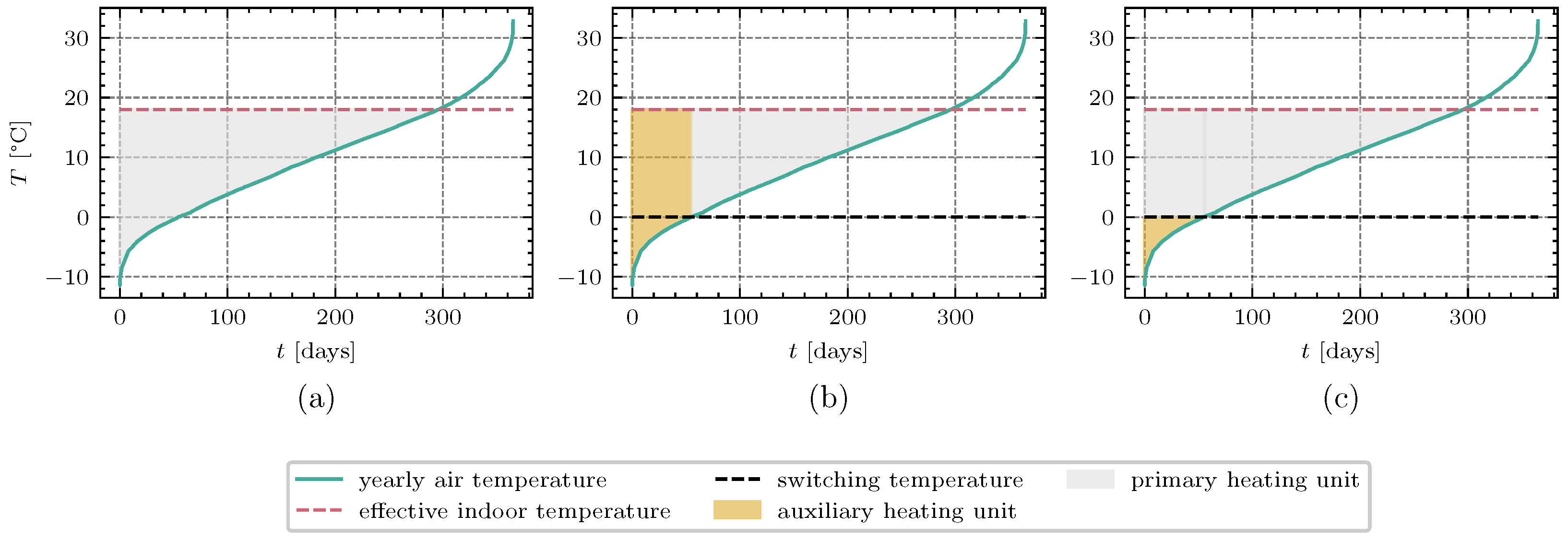
Figure 1 illustrates the yearly distribution of outdoor air temperature at a specific location, indicating how many days per year the daily mean air temperature is at or below a given value. The area between this curve and the effective indoor temperature represents heating degree days ($HDD$), measured in K day. A heating system can consist of a single unit that independently supplies the heating load (Figure 1a), operating in monovalent mode. However, a bivalent heating system includes both a primary and an auxiliary unit. The auxiliary unit can provide the entire heating load below certain outdoor air temperatures in bivalent alternate operation (Figure 1b), or it can supply part of the heating load in bivalent parallel operation (Figure 1c).

A heat pump in a bivalent heating system, often referred to as a hybrid heat pump (HHP), can be supported by various auxiliary heating systems, including solar thermal collectors [4], hybrid photovoltaic–thermal solar collectors [5], district heating [6], biomass boilers [7], and, most commonly, a condensing gas boiler. HHPs provide substantial value in cold climates by reducing peak electricity costs [8] and can contribute to the energy flexibility of a building by enabling load shifting from the heat pump to the auxiliary unit in response to grid necessity [9]. Alternatively, dual-source heat pumps can combine two renewable heat sources, such as outdoor air and ground, to improve operational flexibility and overcome limitations associated with a single heat source [10].

Systems supported by a condensing gas boiler have been most widely studied numerically in various contexts, including single-family houses [11,12,13,14,15,16], multi-family buildings [17,18], and office/commercial buildings [19]. The primary objective in most research has been to evaluate reductions in primary energy consumption, operating costs, and greenhouse gas (GHG) emissions compared to conventional condensing gas boilers. For sensitivity analysis, parameters such as system configurations, climatic conditions, control strategies, electricity generation carbon intensity, and energy prices are typically considered.

Numerical analysis of bivalent parallel–alternate operation of an ASHP and a gas boiler was conducted by Klein et al. [11] for both unrenovated (389 W/K) and renovated (222 W/K) single-family buildings in Germany. Their study concluded that a HHP can reduce primary energy consumption by up to 12% in unrenovated buildings and 26% in renovated buildings when an undersized heat pump is used, compared to heating exclusively with a condensing gas boiler.

Bonomolo et al. [12] analysed the impact of different climatic conditions on the environmental and economic performance of a HHP operating in parallel–alternate mode. They proposed a control strategy based on a $COP$ threshold below which the gas boiler is activated. In a mild climate (Palermo), a monovalent heat pump reduced CO₂ emissions by 40% compared to a gas boiler, while in a moderate climate (Milano), a 25% reduction was achieved with a HHP and a $COP$ switching threshold of 2.3. Similarly, Tihana et al. [13] investigated the operation of a HHP supported by a gas boiler under economic and ecological control strategies, demonstrating that the preferred heat source and switching conditions depend on energy prices and the CO₂ emission intensity of electricity production.

Di Perna et al. [14] experimentally evaluated the $COP$ of an ASHP as a function of outdoor air temperature and humidity to account for the $COP$ reduction caused by defrosting, as well as the efficiency of a condensing gas boiler at different heat loads, in their numerical study of a HHP.

Research by Saffari et al. [15] indicates that HHPs and monovalent ASHPs significantly improve efficiency over conventional boilers, with HHPs achieving slightly higher primary energy savings (50–72%) than monovalent ASHPs (45–70%). In deep retrofit scenarios, HHP systems reduced the carbon footprint by 74%, compared to 68% for monovalent ASHPs. While full building retrofits did not yield a positive 20-year net present value, both heat pump types offered positive returns on investment when installed alongside thermal upgrades. HHP systems generally provide lower operating costs by leveraging gas under low ambient temperatures to avoid reduced electrical efficiency and high electricity costs.

GHG emissions associated with heating a theoretical house with an ASHP under three different operating modes (monovalent, bivalent parallel, and bivalent alternate) and using three different auxiliary energy types (natural gas, biomass, and an electric heater) were numerically analysed by Buday [16]. Three different fixed carbon intensities of electricity production (307.5 g CO₂ eq./kWh, 35.6 g CO₂ eq./kWh, and 861.1 g CO₂ eq./kWh) were considered. They showed that with low and moderate carbon intensity of electricity production, all operating modes reduced GHG emissions compared to gas combustion, while for high electricity emission factors, heating provided by the gas boiler resulted in lower GHG emissions.

A comparative analysis of residential hybrid heat pumps in Italy and Spain [20] revealed that their economic and environmental effectiveness is highly dependent on national energy prices and the electricity generation mix. In Spain, HHP systems can achieve operational cost savings of up to 50% and carbon emission reductions of up to 60% compared to a condensing boiler alone. In Italy, these benefits are more modest: limited to 20% for costs and 30% for emissions. That study also warned about the importance of heat pump size. To maintain high seasonal performance, the system should operate as much as possible at high capacity ratios, even if this means reducing the share of the heating load provided by the ASHP.

Beccali et al. [21] reviewed 38 case studies involving hybrid heat pumps assisted by natural gas boilers published between 2016 and 2022. They identified two primary control strategies: rule-based control (RBC) and model predictive control (MPC). Both strategies were used equally often in the studied cases. RBC is simpler to implement but offers limited flexibility, while MPC offers greater optimisation potential at the cost of increased computational and hardware complexity. The choice of strategy depends on several factors, including climatic conditions (e.g., outdoor air temperature), local energy tariffs, signal processing, and the optimisation objective (e.g., minimising costs, CO₂ emissions, or primary energy consumption).

An autoregressive forecasting model for short-term hourly heat demand was developed and applied by Bizzarri et al. [22] to determine the optimal operating mode of a hybrid heat pump system, aiming to minimise total operating costs. In non-renovated buildings, the MPC strategy achieved up to 20% lower operating costs compared to standard commercial control methods. In renovated buildings, the performance gap between MPC and commercial control was notably smaller due to reduced thermal variability.

An LCA comparison of a HHP and a condensing gas boiler [23] showed that the HHP reduces GHG emissions by 30%. The environmental impact was lower in most categories for the HHP than for the gas boiler, except for human toxicity, water depletion, and metal depletion.

In all the mentioned studies, yearly average electricity production emission factors were used. However, average emission factors do not reflect the temporal variability of the electricity mix. During periods of high electricity demand, more carbon-intensive generation technologies may be dispatched, leading to higher actual GHG emissions than estimated using annual averages. Therefore, time-dependent emission factors should be considered when evaluating different HHP operating strategies [24].

Biomass-assisted HHPs have received limited attention in the literature. Buday et al. [16] showed that their environmental performance strongly depends on the carbon intensity of electricity production and the selected operating mode. Uche et al. [7] demonstrated that appropriate system configuration and control can reduce operating costs and GHG emissions, while in a subsequent study, Uche et al. [25] found that sizing the heat pump to approximately 60–70% of the peak heating demand provides the best balance between operating cost and environmental performance. A recent review of residential biomass heating technologies also highlighted the potential of biomass-assisted hybrid heat pumps while emphasising the limited number of available studies [26].

Reducing peak power demand plays a crucial role in in maintaining the reliability of low-voltage grids in the current age with the deployment of residential low-carbon technologies, such as heat pumps, electric vehicles, photovoltaic (PV) systems, and battery storage. Higher electrification levels can lead to transformer overloading and voltage violations, requiring costly grid reinforcement. In Germany, grid reinforcement can be avoided if a 40–60% share of HHPs is achieved or if 60–80% of buildings are renovated [27]. The potential of peak demand reduction by a bivalent operation of a HHP was identified by Cholewa et al. [28], who suggested that the heat pump should cover from 70% to 90% of the peak heating demand, while the remaining 10% to 30% is covered by the peak heat source.

Aim and Scope

Based on the literature review, the research question of this study is whether the bivalent partially parallel (parallel–alternate) operation of a HHP supported by a biomass pellet boiler in a single-family residential building can reduce operating costs and GHG emissions compared to a monovalent ASHP. It was motivated by a gap in the research on HHPs supported by biomass boilers pointed out by Uche et al. [25]. In contrast to extensively studied gas-assisted HHPs, the techno-economic and environmental performance of biomass-assisted HHPs remains scarcely investigated. These authors have stated that such a HHP can ensure sustainable heating with the use of local energy sources in rural areas. Even though those areas are usually not associated with poor air quality, temperature inversion in wintertime can increase the level of air pollution caused by biomass combustion [29]. Wood smoke exposure has been associated with adverse health effects, including decreased lung function, increased susceptibility to respiratory infections, worsening of asthma symptoms, and potential cardiovascular impacts, due to systemic responses triggered by inhaled particles [30]. Therefore, this study also investigates the potential of HHPs for particulate matter (with a diameter of 10 $\mathsf{\mu }$m or smaller—${\mathrm{PM}}_{10}$) emission reduction compared to a monovalent biomass boiler, an environmental aspect that has received limited attention in previous HHP studies.

The analysis specifically targets buildings that have not yet undergone energy efficiency renovations but are already equipped with a biomass boiler. In retrofit scenarios where an ASHP is added, the existing biomass boiler can serve as an auxiliary heating unit. Consequently, investment costs are excluded from this assessment. Roccatello et al. [31] indicated that in such buildings, hybrid heating systems could be a viable solution for increasing energy efficiency. Furthermore, buildings in rural areas were identified as having greater potential for energy savings compared to buildings in urban areas, driven by their ageing building stock and higher levels of energy poverty [32].

A rule-based control strategy for switching between the ASHP and biomass boiler was developed to determine the optimal cut-off temperature by minimising operating costs under the new electricity distribution tariff methodology. The resulting operation is additionally evaluated using time-dependent electricity production emission factors and PM₁₀ emissions from biomass combustion. The objective of this study is not to precisely model heating demand in an existing building, but rather to evaluate the performance of bivalent heating across a wide range of climatic conditions and building types. Consequently, the model incorporates hourly outdoor air temperature data from 23 representative locations across Slovenia, capturing the country’s diverse climatic conditions. This enables a spatial analysis of how regional climate influences the effectiveness of bivalent ASHP operation. The results were visualised using Geographic Information System (GIS) tools to identify areas where bivalent operation offers significant advantages over monovalent ASHP systems.

The main contributions of this study are the development and validation of a modelling framework for identifying the cost-optimal operation of a biomass-assisted HHP; the combined assessment of operating costs, time-dependent GHG emissions, and PM₁₀ emissions under the new electricity distribution tariff methodology; and the generalisation of the results across different building heat-loss characteristics and climatic conditions with spatial analysis. This approach enables the economic and environmental suitability of biomass-assisted bivalent heating to be assessed at both the building and regional levels.

2. Methodology

This section describes the methodology used to evaluate the bivalent operation of an ASHP and a biomass pellet boiler. First, the developed bivalent heating model and the modelling of the ASHP and climatic conditions are presented, followed by model validation and uncertainty analysis. Subsequently, the calculations of operating costs and GHG and PM₁₀ emissions are described, together with the methodology used to derive and spatially present the results using GIS.

2.1. Bivalent Heating Model

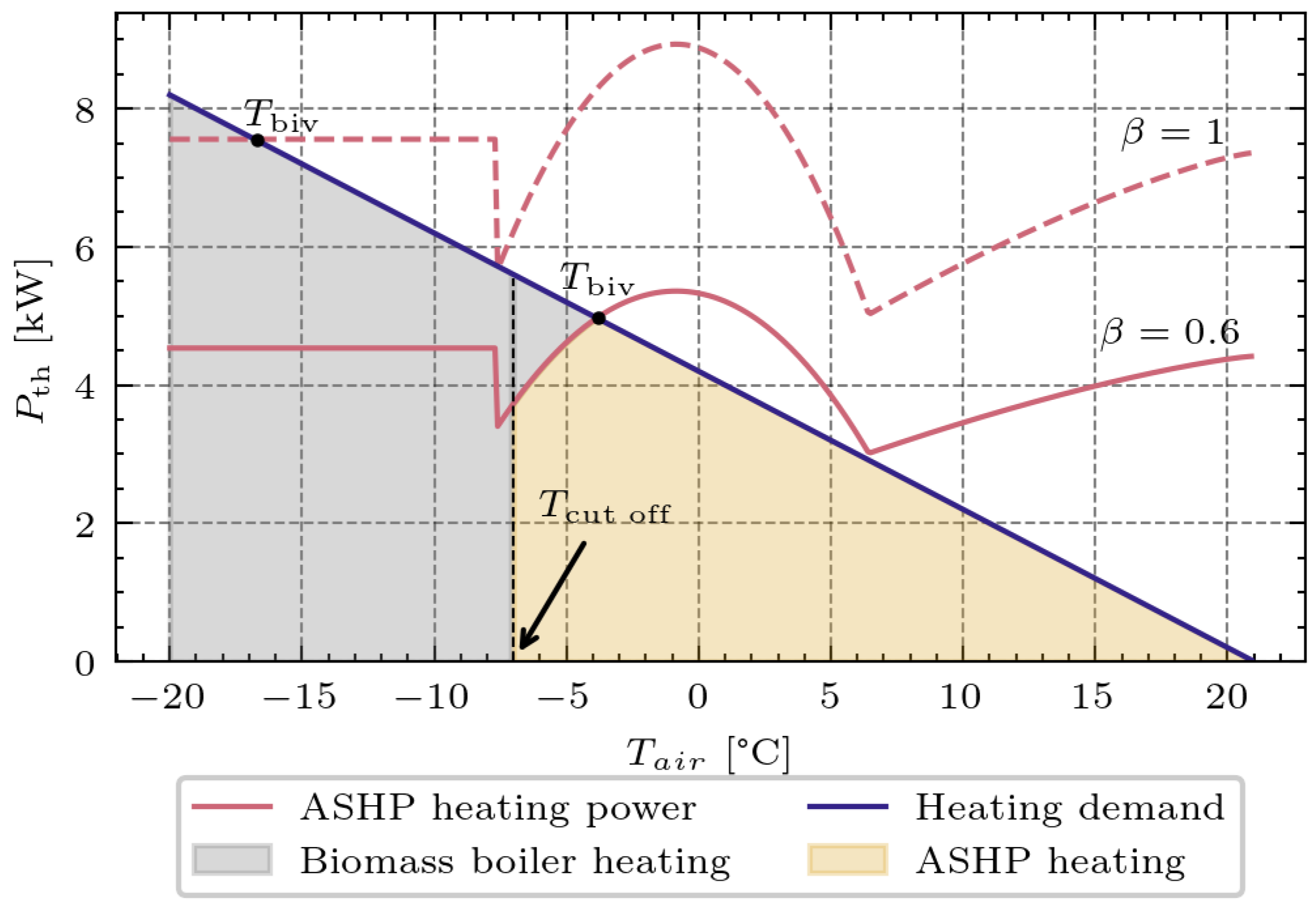
Figure 2 illustrates the operation of the studied hybrid heat pump based on the serial configuration proposed by Uche et al. [7]. The building heating demand and the heating output of a regulated ASHP for two peak load ratios $\beta$ are plotted as functions of outdoor air temperature. The peak load ratio is defined as the ratio between the designed heat pump capacity and the building’s peak heating demand. In the case of a monovalent ASHP ($\beta =1$), the heat pump meets the heating demand on the coldest days but is oversized for most of the year. When the HHP is supported by a biomass pellet boiler, the ASHP capacity can be reduced, as also demonstrated in previous studies [11,25]. The system operates in three temperature-dependent modes. Below the cut-off temperature, the ASHP is switched off and the biomass boiler supplies the entire heating demand. Between the cut-off and bivalent temperatures, both units operate simultaneously, with the ASHP given priority and the biomass boiler covering the remaining heating demand. Above the bivalent temperature, the ASHP alone satisfies the heating demand. According to Uche et al. [25], a peak load ratio of approximately $\beta =0.6$ provides favourable performance in cold climates and was therefore adopted in this study.

A Python (version 3.14.6)-based model was developed to determine the optimal cut-off temperature for the partially parallel operation of the ASHP and biomass pellet boiler. Cut-off temperatures between −20 °C and 15 °C were evaluated with a step size of 0.1 °C, and the value resulting in the lowest total energy cost was identified as optimal. Heating demand and ASHP performance at each timestamp were simulated using the heat pump model described in Section Heat Pump Model and Climatic Data. For the biomass pellet boiler, an efficiency of 79% ± 0.3% was assumed [34].

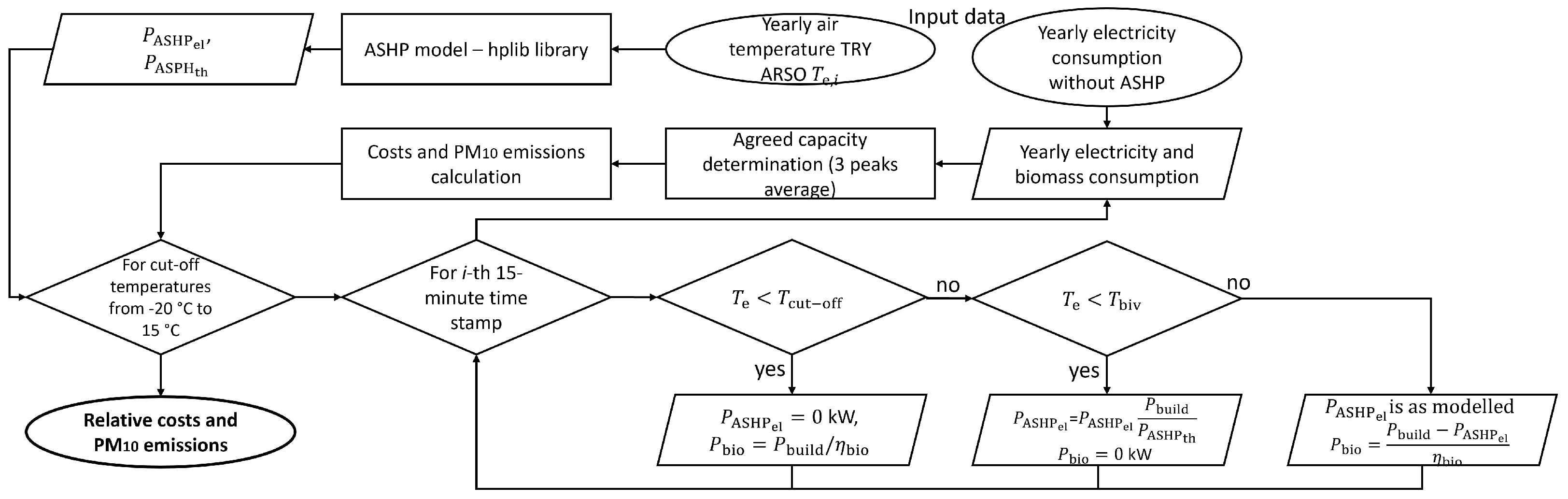
The flow chart of the developed model is shown in Figure 3. For each timestamp in the year, the operating mode is selected according to the outdoor air temperature, cut-off temperature, and bivalent temperature, following the operating strategy described above. In boiler-only operation, the ASHP electricity consumption is set to 0 kW and the biomass input power is calculated from the building heating demand and boiler efficiency. When the ASHP alone can satisfy the heating demand, its modelled electrical power is scaled according to the ratio between the building heating demand and the modelled ASHP thermal output. During simultaneous operation, the ASHP operates at its modelled output and the biomass boiler supplies the remaining heating demand. Additional constraints were implemented based on model validation: (1) the heating season was defined as proposed by the Slovenian Environment Agency (ARSO) (it begins on the fourth day after three consecutive days when the air temperature at 21:00 is below 12 °C in the second half of the year, and ends on the fourth day after three consecutive days when the temperature at 21:00 exceeds 12 °C in the first half of the year); (2) if the outdoor temperature over a timestamp is higher than 15 °C, heating is not required; (3) if the daily mean outdoor temperature during the heating season is above 10 °C, heating is not required; (4) if the daily mean outdoor temperature during the second half of the year and within the heating season is above 7 °C, heating is not required. Annual electricity consumption of the ASHP was added to the annual electricity consumption of the household without a heat pump. Finally, energy costs, GHG emissions related to electricity consumption, and PM₁₀ emissions associated with biomass combustion were calculated. The algorithm was repeated for each cut-off temperature between −20 °C and 15 °C. The results are presented as relative operating costs and GHG emissions compared to monovalent heating with an ASHP ($\beta =1$) as a function of the cut-off temperature. The optimal cut-off temperature was identified as the value at which the total energy cost was minimised. PM₁₀ emissions at the optimal cut-off temperature are presented similarly but relative to monovalent heating with a biomass boiler.

Heat Pump Model and Climatic Data

The electricity consumption, thermal power, and $COP$ of an air-source heat pump were modelled using the open-access Python-based library hplib [33]. The library’s database collects data from laboratory tests for 506 heat pumps (outdoor air–water-, brine–water-, and water–water-regulated or on/off) from 30 different manufacturers, available in [35]. Efficiency parameters can be calculated for a specific model or one of six predefined generic heat pump types using a least-squares regression model, consistent with the approach presented in [36]. The model requires time-series inputs of primary input temperature, secondary input temperature, and indoor air temperature to simulate the $COP$, electricity consumption, and thermal power of the ASHP.

For this study, simulations were conducted using a generic regulated ASHP across various total heat loss coefficients $H_{\mathrm{tot}}$ and building locations in Slovenia. Accordingly, the rated thermal power of the ASHP in each case was calculated using Equation (1), as follows:

$$P_{\mathrm{HP},\mathrm{th}}=\beta H_{\mathrm{tot}}\left(T_{\mathrm{in}}-T_{\mathrm{e},\mathrm{d}}\right),$$

(1)

where $T_{\mathrm{in}}$ is the desired indoor temperature (21 °C) and $T_{\mathrm{e},\mathrm{d}}$ is the design’s outdoor air temperature, specific to each location. Seven different $H_{\mathrm{tot}}$ values were assumed, ranging from 100 W/K to 400 W/K with 50 W/K increments. The analysis includes 23 locations across Slovenia for which ARSO provides hourly meteorological data in the form of a typical reference year (TRY) [37]. Hourly time series of outdoor air temperature $T_{\mathrm{e}}$ were used as the model input for both ambient and primary input temperatures, as they are equivalent for an ASHP. Secondary input temperature was defined as the actual flow temperature in the heating system and was calculated using Equation (2) [38], as follows:

$$T_{\mathrm{hs},\mathrm{f}}=T_{\mathrm{in}}+{\displaystyle \frac{T_{\mathrm{hs},\mathrm{f},\mathrm{d}}-T_{\mathrm{hs},\mathrm{r},\mathrm{d}}}{2}}·{\displaystyle \frac{T_{\mathrm{in}}-T_{\mathrm{e}}}{T_{\mathrm{in}}-T_{\mathrm{e},\mathrm{d}}}}+\left({\displaystyle \frac{T_{\mathrm{hs},\mathrm{f},\mathrm{d}}+T_{\mathrm{hs},\mathrm{r},\mathrm{d}}}{2}}-T_{\mathrm{in}}\right)·{\left({\displaystyle \frac{T_{\mathrm{in}}-T_{\mathrm{e}}}{T_{\mathrm{in}}-T_{\mathrm{e},\mathrm{d}}}}\right)}^{1/m},$$

(2)

where $T_{\mathrm{hs},\mathrm{f},\mathrm{d}}$ is the designed heating system flow temperature (55 °C), $T_{\mathrm{hs},\mathrm{r},\mathrm{d}}$ is the designed heating system return temperature (45 °C), and m is the heating system exponent (1.3). Simulated hourly time series of electricity consumption, thermal output, and $COP$ were subsequently interpolated to 15 min intervals to align with the temporal resolution of the measured grid electricity consumption data.

2.2. Model Validation and Uncertainty Analysis

Validation was conducted using the case of an uninsulated single-family house ($H_{\mathrm{tot}}$ = 350 W/K) built in the 1970s with a heated area of 200 m² located near the Lesce Airport meteorological station. In 2023, the building’s heating system was retrofitted, replacing the condensing gas boiler with an ASHP rated at 13.8 kW of thermal power. Simultaneously, a 14.8 kW solar photovoltaic (PV) system was installed under a net-metering financial scheme. As a result, the electricity distribution company provided only net electricity taken from and fed into the grid at 15 min intervals. Actual consumption at each timestamp, $P_{\mathrm{cons}}$, was calculated using PV production data, $P_{\mathrm{PV}}$, together with the electricity taken from and fed into the grid, using Equation (3) as follows:

$$P_{\mathrm{cons}}=P_{\mathrm{PV}}+P_{\mathrm{from},\mathrm{grid}}-P_{\mathrm{to},\mathrm{grid}}.$$

(3)

However, due to the lack of synchronisation between the datasets, negative consumption values were occasionally produced at certain timestamps. Therefore, validation was performed using daily average data instead.

The ASHP’s electrical power, $COP$, and thermal output were simulated as described in Section 2.1, using hourly outdoor air temperature data from the Lesce Airport meteorological station for the year 2024. Since only total electricity consumption was available, the non-heating electricity demand was estimated from data for the year 2022—the last full year without a heat pump. A comparison of the electricity consumption during the summer season in 2022 and 2024 showed higher consumption in 2022 (3186 kWh vs. 2506 kWh, respectively). This reduction was attributed primarily to changes in household occupancy and the replacement or removal of several electrical appliances. To account for this difference, the 2022 non-heating electricity profile was scaled by the ratio of the non-heating electricity consumption in 2024 and 2022 (21.3% reduction). The adjusted 2022 consumption was then summed with the modelled ASHP electricity consumption and compared to the actual measured total electricity consumption in 2024.

Uncertainty Analysis

In general, the accuracy of variable x is calculated using Equation (4), as follows:

$$u\left(x(y_1,y_2,\dots ,y_n)\right)=\sqrt{{\left(\frac{\partial x}{\partial y_1}u\left(y_1\right)\right)}^2+{\left(\frac{\partial x}{\partial y_2}u\left(y_2\right)\right)}^2+\dots +{\left(\frac{\partial x}{\partial y_n}u\left(y_n\right)\right)}^2}.$$

(4)

Tariffs for electricity and biomass, as well as measured electricity consumption, were assumed to be exact values. Random uncertainty of the modelled electric and thermal power at each timestamp during the heating season was attributed to the uncertainty of the heat pump model and was calculated using Equation (5), as follows:

$$u{\left(P\right)}_i=P_i·MARE,$$

(5)

where MARE refers to the mean absolute relative error. The value for the modelled electricity consumption of the ASHP, $MAR{E}_{\mathrm{el}}$, was assumed to be 0.195, while the value for the modelled thermal power of the heat pump, $MAR{E}_{\mathrm{th}}$, was assumed to be 0.235. Both values were obtained from the documentation of the hplib model for regulated ASHPs [33].

Random uncertainty of yearly energy consumption was calculated using Equation (6), as follows:

$$u_{\mathrm{rand}}\left(E\right)=\sqrt{\sum _{i=1}^N{\left({\displaystyle \frac{u\left(P_i\right)}{4}}\right)}^2},$$

(6)

where $u\left(P_i\right)$ is the uncertainty of the ASHP thermal or electrical power at the i-th timestamp, and N is the number of data points, both during the heating season. Systematic uncertainty of electricity consumption was associated with the deviation in non-heating electricity consumption and was calculated using Equation (7), as follows:

$$u_{\mathrm{sys}}\left(E\right)=t_{\mathrm{y}}\sqrt{{\left(s\left(P_{\mathrm{el},\mathrm{cons},2022}\right)/M_{2022}\right)}^2+{\left(s\left(P_{\mathrm{el},\mathrm{cons},2024}\right)/M_{2024}\right)}^2},$$

(7)

where $s\left(P_{\mathrm{el},\mathrm{cons}}\right)$ is the standard deviation of the electricity consumption measurements over each respective year, M is the number of measurements during the heating season, and $t_{\mathrm{y}}$ is the number of hours in a year (8760 h). The calculated systematic uncertainty of yearly electricity consumption in this analysis is 144.5 kWh. Overall uncertainty of yearly electricity consumption was then calculated using Equation (8), as follows:

$$u\left(E\right)=\sqrt{u_{\mathrm{rand}}{\left(E\right)}^2+u_{\mathrm{sys}}{\left(E\right)}^2}.$$

(8)

Daily values of the electricity production carbon intensity factor, $f_{{\mathrm{CO}}_2}$, were obtained from Electricity Maps [39] for the years 2021–2024. Uncertainty of the electricity production carbon intensity factor at each timestamp was calculated using Equation (9), as follows:

$$u{\left(f_{{\mathrm{CO}}_2}\right)}_i=s{\left(f_{{\mathrm{CO}}_2}\right)}_i/N_i,$$

(9)

where $s{\left(f_{{\mathrm{CO}}_2}\right)}_i$ is the standard deviation of the carbon intensity factor at timestamp i, and $N_i$ is the number of data points available for each timestamp ($N_i=4$).

2.3. Cost and PM₁₀ Emission Calculation

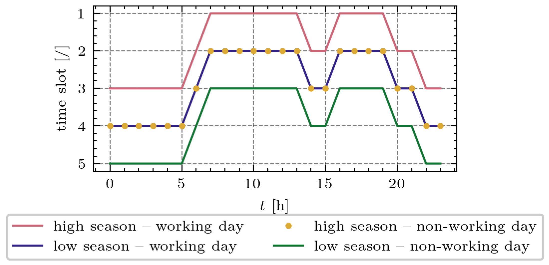
The electricity distribution cost was calculated using the new methodology proposed by the Energy Agency and adopted in an act that entered into force in October 2024 [40]. Although the act defines the methodology for all consumers, the specific methodology and charges presented and used in this work apply to household consumers on the distribution grid. A new methodology was already presented by Kopač [41]. It introduces three different time slots within a day, distinguishing between working and non-working days and between the high season (November–February) and the low season (March–October). In total, five distinct time slots with corresponding charges are defined and presented in Figure 4 and

Table 1. Agreed capacity and energy charge for electricity distribution cost in 2024 proposed by the new methodology [42].

Time Slot b	1	2	3	4	5
Agreed capacity tariff $T{d}_b^C$ [EUR/kW]	3.61324	0.88240	0.19137	0.01316	0
Energy tariff $T{d}_b^E$ [EUR/kWh]	0.01958	0.01844	0.01837	0.01838	0.01847

. Instead of the nominated capacity, the new methodology introduces the agreed capacity for each time slot based on the average of the three peaks from the previous winter season. However, consumers can adjust the agreed capacity in advance of each month. Moreover, the agreed capacity of each time slot must be greater than or equal to that of the preceding time slot, making the first time slot the one with the lowest agreed capacity.

Consumer electricity consumption is measured every 15 min as the average power over the interval. If the average power $C{m}_{k,b}$ of the k-th measurement in time slot b exceeds the agreed capacity $C{c}_b$, the additional monthly excess power cost for that time slot, $OMR{d}_b^{C_{\mathrm{ex}}}$, is calculated and charged with Equation (10), as follows:

$$OMR{d}_b^{C_{\mathrm{ex}}}=F_{\mathrm{ex}}·T{d}_b^C\sqrt{\sum _{K=1}^n{\left(C{m}_{k,b}-C{c}_b\right)}^2},$$

(10)

where $F_{\mathrm{ex}}$ is the weighting factor for excess power (0.9 in 2024 and 2025, 1.05 in 2026 and 2027, and 1.2 from 2028 onward), $T{d}_b^C$ is the capacity tariff for time slot b, and n is the number of measurements exceeding the agreed capacity. The total monthly electricity distribution cost $OMRd$ is then obtained by summing all time slots according to Equation (11), as follows:

$$OMRd={\displaystyle \sum _{b=1}^5}\left(OMR{d}_b^{C_{\mathrm{ex}}}+T{d}_b^C·C{c}_b+T{d}_b^E·c{e}_b\right),$$

(11)

where $c{e}_b$ is the energy consumed from the distribution grid during time slot b. In addition to distribution cost, the total electricity cost for households also includes the cost of energy, as well as charges related to renewable energy sources (RES) and cogeneration of heat and electricity taxes. These are calculated by multiplying monthly energy consumption by the corresponding tariffs. A similar approach is used to calculate the cost of biomass pellets. All electricity tariffs listed in

Table 2. Energy tariffs used for cost calculation.

Electricity—energy tariff [EUR/kWh]	0.097	[1]
Electricity—RES and CHP tax tariff [EUR/kWh]	0.0183	[1]
Biomass pellet price [EUR/kWh]	0.06941	[43]

are provided by the Statistical Office (SURS) [1] as average prices for households in 2022 and 2023, excluding VAT, while the biomass pellet price is provided by the Forestry Institute [43].

In the analysis, dynamic emission intensity factors $f_{{\mathrm{CO}}_{2,\mathrm{el}}}$ for electricity production in Slovenia were used, as provided by Electricity Maps [39]. The average daily emission factor was calculated based on daily data for the years 2021–2024. Each timestamp i was assigned the corresponding emission intensity factor, and emissions related to electricity consumption were calculated with Equation (12), as follows

$$C{F}_{\mathrm{el},i}=f_{{\mathrm{CO}}_2,\mathrm{el},i}·P_{\mathrm{el},i}/4.$$

(12)

The equation is divided by 4 to convert the electricity consumption from 15 min intervals into kWh. Biomass is proposed as a CO₂-neutral fuel. For the calculation of PM₁₀ emissions related to biomass combustion, the PM₁₀ emission factor $f_{{\mathrm{PM}}_{10},\mathrm{bio}}$ for a biomass pellet boiler is assumed to be 170 mg/kWh ± 33 mg/kWh [44]. Therefore, the yearly PM₁₀ emissions of a heating system can be calculated with Equation (13), as follows:

$$P{M}_{10}=E_{\mathrm{bio}}{f}_{{\mathrm{PM}}_{10},\mathrm{bio}}={\displaystyle \frac{E_{\mathrm{th}}{f}_{{\mathrm{PM}}_{10},\mathrm{bio}}}{{\eta }_{\mathrm{bio}}}}.$$

(13)

2.4. Presentation of Results with GIS

2.4.1. Relative Savings Compared to Monovalent ASHP

The yearly electricity consumption of an ASHP for heating in a bivalent heating system can be calculated with Equation (14), as follows:

$$E_{\mathrm{el},\mathrm{ASHP}}={\displaystyle \frac{\epsilon E_{\mathrm{th}}}{CO{P}_{\mathrm{s},\mathrm{biv}}}}={\displaystyle \frac{\epsilon H_{\mathrm{tot}}HDD}{CO{P}_{\mathrm{s},\mathrm{biv}}}},$$

(14)

where $CO{P}_{\mathrm{s}}$ is the seasonal coefficient of performance and $\epsilon$ is the ratio of heating provided by the ASHP in the bivalent heating system. Relative operational cost savings, $C_{\mathrm{rel}}$, can therefore be expressed with Equation (15), as follows:

$$C_{\mathrm{rel}}=1-{\displaystyle \frac{c_{\mathrm{el}}\left(\frac{\epsilon H_{\mathrm{tot}}HDD}{CO{P}_{\mathrm{s},\mathrm{biv}}}+E_{\mathrm{el},\mathrm{rest}}\right)+c_{\mathrm{bio}}(1-\epsilon )\frac{H_{\mathrm{tot}}HDD}{{\eta }_{\mathrm{bio}}}}{c_{\mathrm{el}}\left(\frac{H_{\mathrm{tot}}HDD}{CO{P}_{\mathrm{s},\mathrm{mono}}}+E_{\mathrm{el},\mathrm{rest}}\right)}},$$

(15)

Moreover, relative GHG emission reductions, $GH{G}_{\mathrm{rel}}$, can be calculated with Equation (16), as follows:

$$GH{G}_{\mathrm{rel}}=1-{\displaystyle \frac{f_{{\mathrm{CO}}_2,\mathrm{el}}\left(\frac{\epsilon H_{\mathrm{tot}}HDD}{CO{P}_{\mathrm{s},\mathrm{biv}}}+E_{\mathrm{el},\mathrm{rest}}\right)}{f_{{\mathrm{CO}}_2,\mathrm{el}}\left(\frac{H_{\mathrm{tot}}HDD}{CO{P}_{\mathrm{s},\mathrm{mono}}}+E_{\mathrm{el},\mathrm{rest}}\right)}},$$

(16)

where $E_{\mathrm{el},\mathrm{rest}}$ is the yearly non-heating electricity consumption (8788 kWh). $\epsilon$, $CO{P}_{\mathrm{s},\mathrm{biv}}$, and $CO{P}_{\mathrm{s},\mathrm{mono}}$ are not constant values but functions of $HDD$. The fitting physical model for both relative reductions can therefore be written using Equations (17) and (18), as follows:

$$C_{\mathrm{rel}}=1-{\displaystyle \frac{\frac{\epsilon \left(HDD\right)A_1}{CO{P}_{\mathrm{s},\mathrm{biv}}\left(HDD\right)}HDD+\epsilon \left(HDD\right)A_2+A_3}{\frac{A_4}{CO{P}_{\mathrm{s},\mathrm{mono}}\left(HDD\right)}HDD+A_5}},$$

(17)

$$GH{G}_{\mathrm{rel}}=1-{\displaystyle \frac{\frac{\epsilon \left(HDD\right)A_1}{CO{P}_{\mathrm{s},\mathrm{biv}}\left(HDD\right)}HDD+\epsilon \left(HDD\right)A_2}{\frac{A_3}{CO{P}_{\mathrm{s},\mathrm{mono}}\left(HDD\right)}HDD+A_4}}.$$

(18)

All of $\epsilon \left(HDD\right)$, $CO{P}_{\mathrm{s},\mathrm{biv}}\left(HDD\right)$, and $CO{P}_{\mathrm{s},\mathrm{mono}}\left(HDD\right)$ can be assumed to be linear functions. Under this assumption, the physically based formulation represents a non-linear rational function that was fitted to the data. In addition, first- and second-order polynomial models were evaluated for comparison.

The coefficients of determination, $R^2$, obtained for the physical, linear, and quadratic models are summarised in

Table 3. Coefficients of determination $R^2$ obtained for the physical, linear, and quadratic models ($H_{\mathrm{tot}}=300$ W/K).

Model	Cost Reduction	GHG Reduction
physical	0.86	0.89
linear	0.91	0.87
quadratic	0.94	0.89

. The second-order polynomial exhibited a goodness-of-fit comparable to that of the physically based formulation across all analysed cases. Owing to its simplicity, reduced parameterisation, and ease of application, the quadratic model was selected for subsequent analyses. However, the applicability of the empirical quadratic model is limited to the calibration range.

2.4.2. Absolute PM₁₀ Emission Reduction

On the other hand, the absolute PM₁₀ emission reductions are calculated compared to a monovalent biomass boiler and can be written as Equation (19), as follows:

$$P{M}_{10,\mathrm{red}}={\displaystyle \frac{(1-\epsilon \left(HDD\right))f_{{\mathrm{PM}}_{10},\mathrm{bio}}{H}_{\mathrm{tot}}}{{\eta }_{\mathrm{bio}}}}HDD.$$

(19)

Again, $\epsilon \left(HDD\right)$ is assumed to be a linear function, so in this case, the physical model can be written as a second-order polynomial with Equation (20), as follows:

$$P{M}_{10,\mathrm{red}}\left(HDD\right)=a_{1}HD{D}^2+a_{2}HDD+a_3.$$

(20)

The results and fitted functions were evaluated separately for the seven analysed total heat loss coefficients, $H_{\mathrm{tot}}$, and plotted against heating degree day values. The optimal fitted function was determined using a Monte Carlo simulation with 10⁴ iterations to account for uncertainty in the data. In each iteration, new $HDD$ and savings/reduction data were generated for each analysed location within their corresponding uncertainty and assuming a normal probability distribution. For each simulated dataset, a new second-order polynomial was fitted. The final fitted function was obtained as the mean of all the fitted polynomials, while the associated uncertainty bounds were defined by the 16th and 84th percentiles, corresponding to a 68% confidence interval. Additionally, the lower and upper $HDD$ limits of applicability of the fit were defined: the upper limit was 8000 K day (data range), and the lower limit was the $HDD$ value below which bivalent heating no longer reduces operating costs (first positive root of $C_{\mathrm{rel}}\left(HDD\right)$).

According to Stegnar et al. [45], a typical single-family building in Slovenia built between 2003 and 2008 and that has not implemented any energy renovation measures has a heated floor area of 160 m² and a specific annual heat demand of 120 kWh/m². For a location where $HDD$ is 2800 K day, the heat loss coefficient was estimated at 286 W/K. Therefore, the heat loss coefficient, $H_{\mathrm{tot}}$, was assumed to be 300 W/K for the presentation of the possible savings of bivalent operation when a biomass pellet boiler is replaced with an ASHP.

Operating cost savings, GHG, and PM₁₀ emission reductions for this case were visualised using a Geographic Information System (GIS) tool. The analysis employed a raster dataset of average heating degree days for the period 1991–2020, provided by ARSO, with a spatial resolution of 1 km × 1 km. PM₁₀ emission reductions were computed for each raster cell using the relevant fitted functions based on the selected $H_{\mathrm{tot}}$ value and were displayed on a map.

3. Results and Discussion

This section first presents the validation of the developed model against measured electricity consumption. The validated model is then used to evaluate the operating costs and GHG and PM₁₀ emissions of the bivalent heating system in comparison with monovalent ASHP and biomass boiler operation. Finally, the influence of climatic conditions and building heat-loss characteristics is analysed, and the potential PM₁₀ emission reduction is evaluated spatially across Slovenia.

3.1. Model Validation

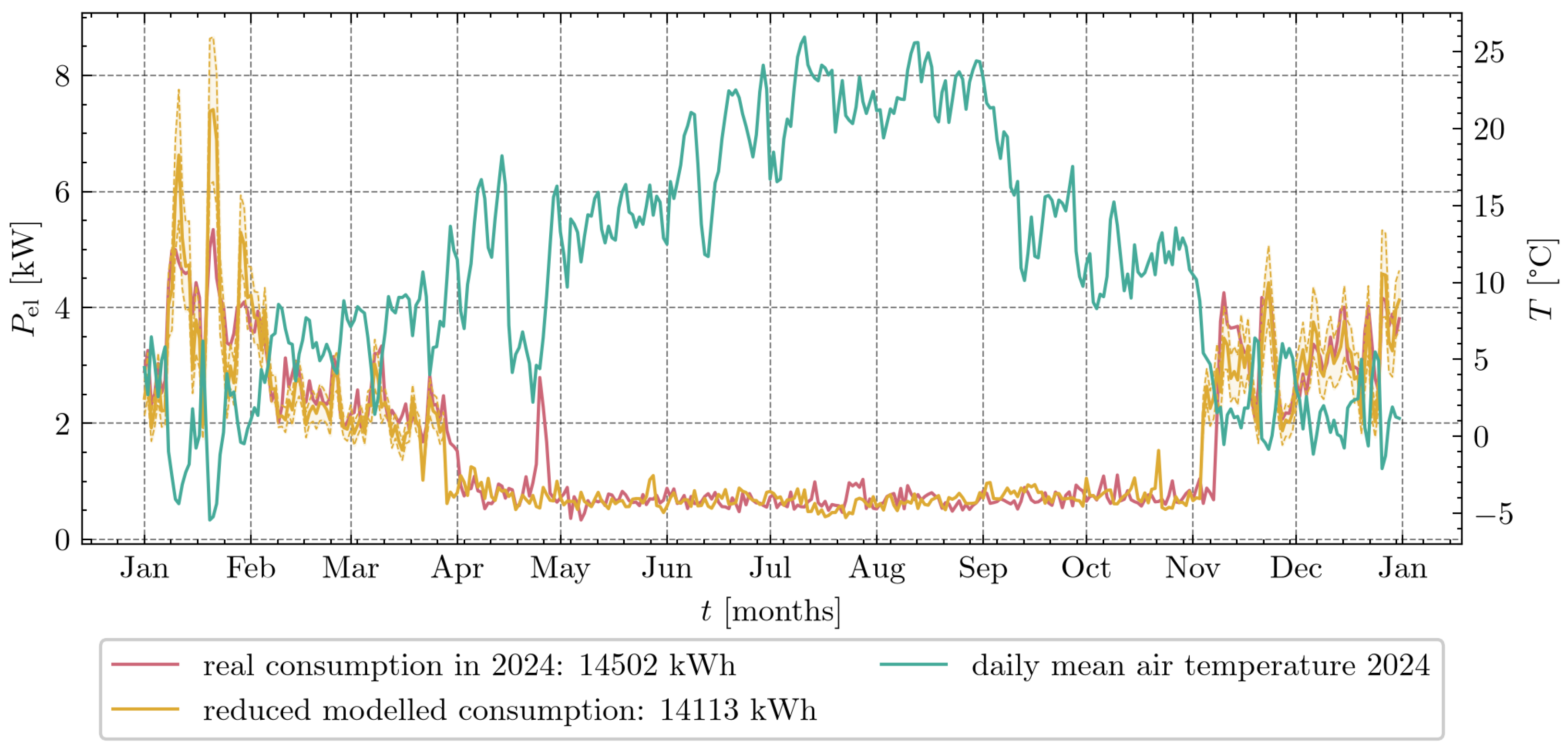
Figure 5 presents the measured electricity consumption (expressed as daily mean power) for 2024, alongside the modelled electricity consumption for the same period and the corresponding daily mean outdoor air temperature. Modelled consumption consists of corrected historical consumption without an ASHP, combined with modelled ASHP consumption. The uncertainty band for energy consumption is shown only for the modelled values during the heating season, as described in Section 2.4.1. The total yearly measured and modelled electricity consumption was 14,502 kWh and 14,113 kWh, respectively, resulting in a deviation of less than 2.7%, as over- and underpredictions partially cancelled out over time. Nevertheless, during the heating season, 66% of measurements fell within the model’s uncertainty band, supporting the predictive adequacy of the model. Notable deviations occurred at the beginning and end of the heating season, which can be attributed to discrepancies between the actual start and end dates of heating operation and those defined by the model. Additionally, supplementary heating provided by the ASHP at the end of April is evident in the figure and corresponds to lower outdoor air temperatures during that period, even though it is outside the heating season.

However, this validation has certain limitations; due to the lack of synchronisation between PV production and grid exchange data, the validation was performed using daily averages rather than 15 min values, so short-term variations could not be directly validated. In addition, non-heating electricity consumption in 2024 was estimated from corrected 2022 data rather than measured separately, introducing additional uncertainty into the validation.

3.2. Relative Savings of Bivalent Heating System

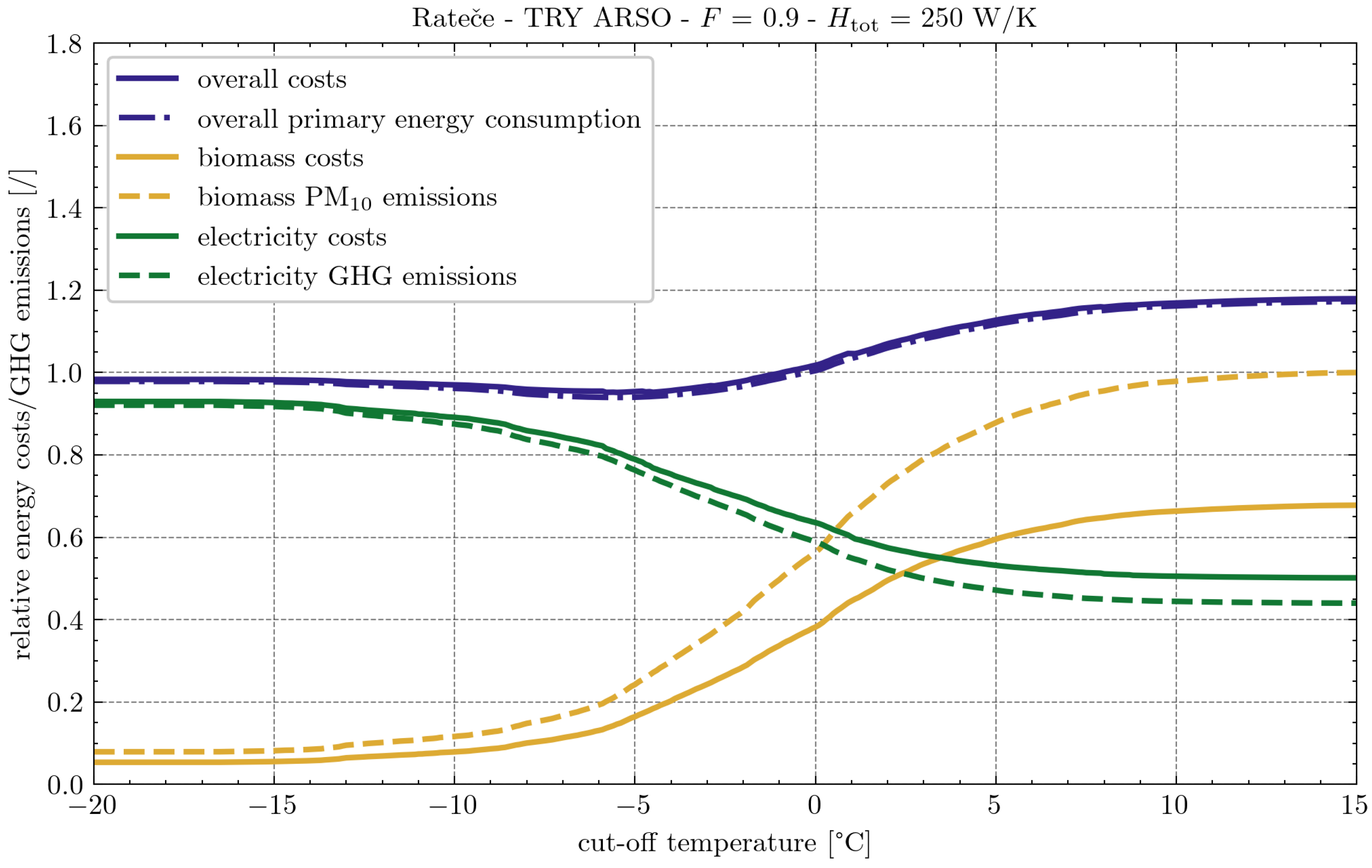
The analysis was conducted for 23 locations and seven total heat loss coefficients. The results are presented as relative operating costs and relative GHG emission reduction compared to a monovalent ASHP, and PM₁₀ emissions in comparison to the monovalent operation of a biomass boiler. These were evaluated separately for electricity consumption, biomass consumption, and overall energy consumption. Figure 6 displays the results for a building in Rateče, assuming a specified $H_{\mathrm{tot}}$ and excess power factor. Relative costs and GHG emissions were shown as functions of the cut-off temperature in the bivalent heating system. At temperatures above 15 °C, no heating was required, so a cut-off temperature of 15 °C corresponds to heating exclusively with the biomass pellet boiler. In this case, replacing the biomass boiler with an ASHP resulted in a reduction in overall energy costs of 18% and a GHG emission reduction of 50%. Further reductions were achieved through bivalent operation of the ASHP and biomass boiler. The lowest operating costs occurred at $T_{\mathrm{switch}}=$ −5.5 °C, yielding an additional 4.8% cost saving relative to monovalent ASHP operation. The GHG emission reduction of the bivalent system at minimal operating costs was 20%. However, an inappropriately selected switching temperature could result in increased energy costs. Specifically, switching temperatures above 0 °C used for cost optimisation may lead to worse performance than monovalent ASHP operation.

Table 4. Effect of excess power factor on results.

	${\mathit{F}}_{\mathbf{ex}}=0.90$	${\mathit{F}}_{\mathbf{ex}}=1.05$	${\mathit{F}}_{\mathbf{ex}}=1.20$
lowest costs
$T_{\mathrm{switch}}$ [°C]	−5.5	−5.5	−5.5
energy costs [EUR]	2711.44	2711.65	2711.86
energy costs [%]	95.2	95.1	95.1
agreed capacity
time slot 1 [kW]	10.7	10.7	10.7
time slot 2 [kW]	11.4	11.4	11.4
time slot 3 [kW]	11.4	11.4	11.4
time slot 4 [kW]	11.4	11.4	11.4
time slot 5 [kW]	11.4	11.4	11.4

compares results obtained using different excess power factors, $F_{\mathrm{ex}}$, for the case described above. An increase in the excess power factor did not lead to an increase in total energy costs and therefore did not affect the relative savings of bivalent operation. This outcome is partly due to the structure of the new methodology, where the agreed capacity for each time slot is defined based on the same electricity consumption being analysed.

Therefore, this study has several limitations from the perspective of operating costs:

• Agreed capacity was calculated based on the same electricity consumption as used in the analysis. In practice, it is determined from peak loads in the previous winter; if the previous winter was unusually cold, excess capacity costs may increase. However, a separate analysis using historical climatic data showed cost reductions of a similar magnitude to those obtained for the corresponding $HDD$ range in Figure 7.
• Operating costs and GHG and PM₁₀ emissions were estimated under the assumption of optimal agreed capacity, whereas real-world consumers may not optimise this value precisely.
• Cut-off temperatures were derived under the assumption of optimal agreed capacity; if the actual agreed capacity is overestimated, the savings from bivalent operation could be higher.

Additionally constant biomass boiler efficiency and PM₁₀ emission factors were assumed. In real bivalent operation, boiler efficiency and particulate emissions may vary with part-load operation and during start-up and shutdown periods. These transient effects are not captured by the present model and may therefore lead to an overestimation of the calculated PM₁₀ emission reductions.

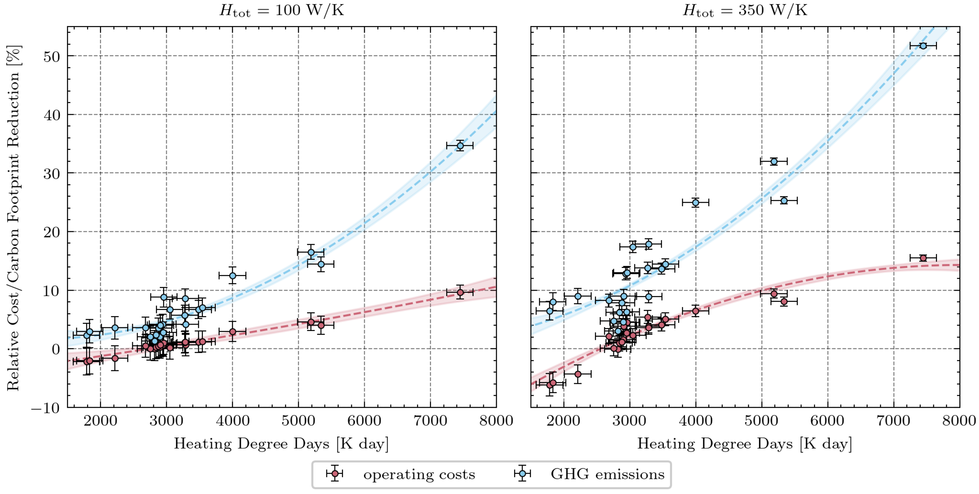
Figure 7 presents relative energy cost savings and GHG emission reductions in the bivalent heating system compared to monovalent operation of an ASHP, calculated at the optimal switching temperature. The results are shown for both insulated (100 W/K) and uninsulated (350 W/K) single-family buildings across the 23 analysed locations. A second-order polynomial function was fitted to represent the dependence of savings on the heating degree day value. For $HDD$ values lower than the positive root of the fitted function, savings were assumed to be 0%. The complete set of fitted functions for each analysed $H_{\mathrm{tot}}$ is provided in Appendix B. The fitted polynomial functions and their coefficients are specific to the analysed Slovenian context, including electricity tariff structure, energy prices, and emission factors. Therefore, the coefficients should not be applied directly to other countries or regions; application of the methodology elsewhere requires re-simulation using local input data and subsequent determination of new fitting coefficients.

In general, GHG emission reductions are approximately three times higher than operating cost savings, and both increase with $HDD$. As expected, relative savings are lower for insulated buildings than for uninsulated buildings because of their lower heating demand. The results show that bivalent heating does not reduce operating costs below $HDD$ values of 2737 K day and 2561 K day for insulated and uninsulated buildings, respectively. Furthermore, for $HDD$ values around 3000 K day, corresponding to most of the analysed locations, operating cost savings are marginal for insulated buildings but reach up to 5% for uninsulated buildings. Even though the bivalent heating system does not reduce operating costs significantly for these locations, GHG emissions can be reduced by up to 10% for insulated buildings and up to 20% for uninsulated buildings.

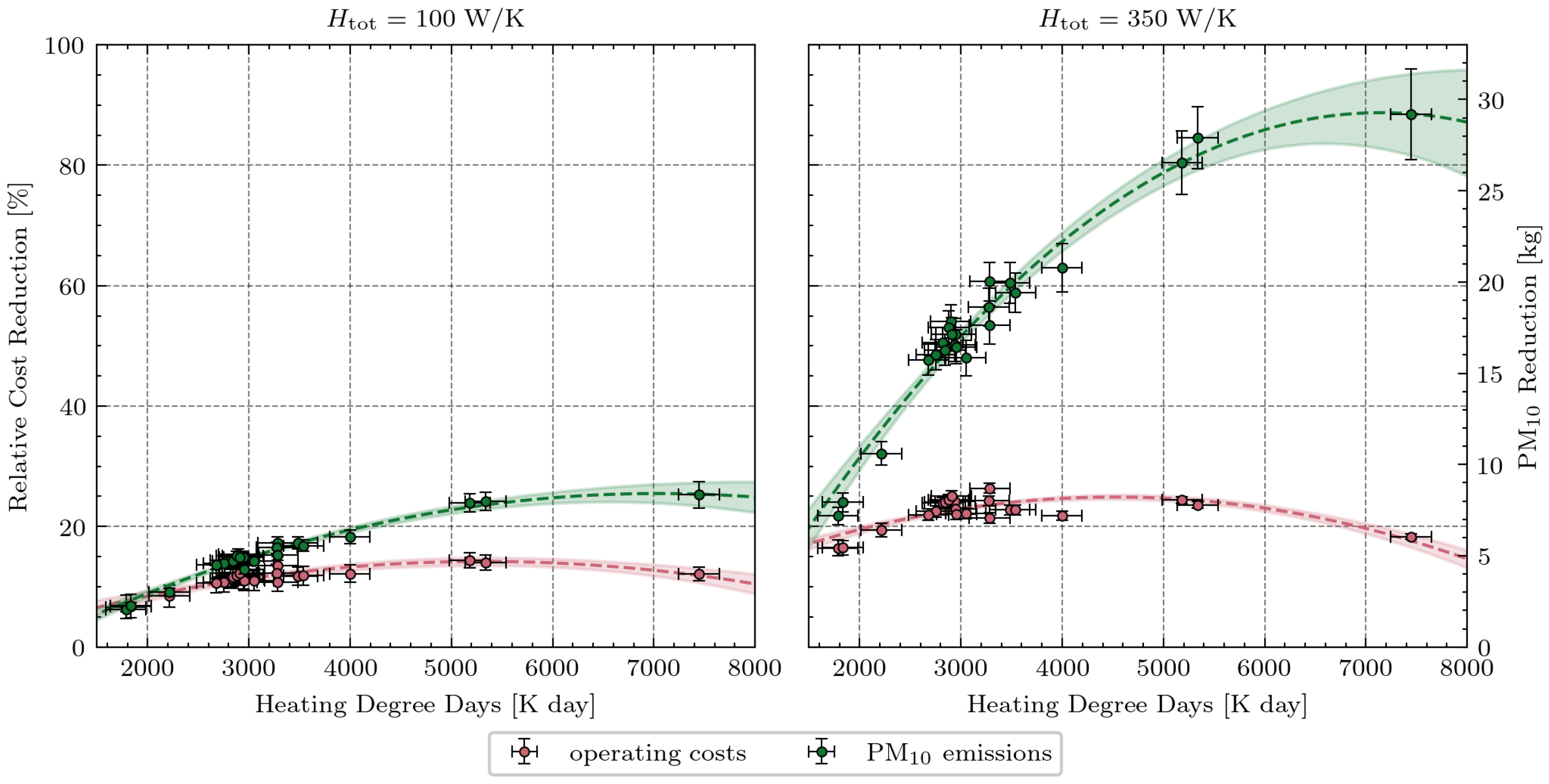
Figure 8 shows absolute PM₁₀ emission reductions and relative operating cost savings of the HHP compared to a monovalent biomass boiler. For most locations, the HHP can reduce operating costs by up to 15% for insulated and up to 25% for uninsulated buildings. In colder locations, the savings are similar, which can be attributed to the lower share of heating provided by the ASHP. For most analysed locations where the HHP reduces operating costs, yearly PM₁₀ emissions can be reduced by 4–7 kg for insulated buildings and by 15–21 kg for an uninsulated single-family building.

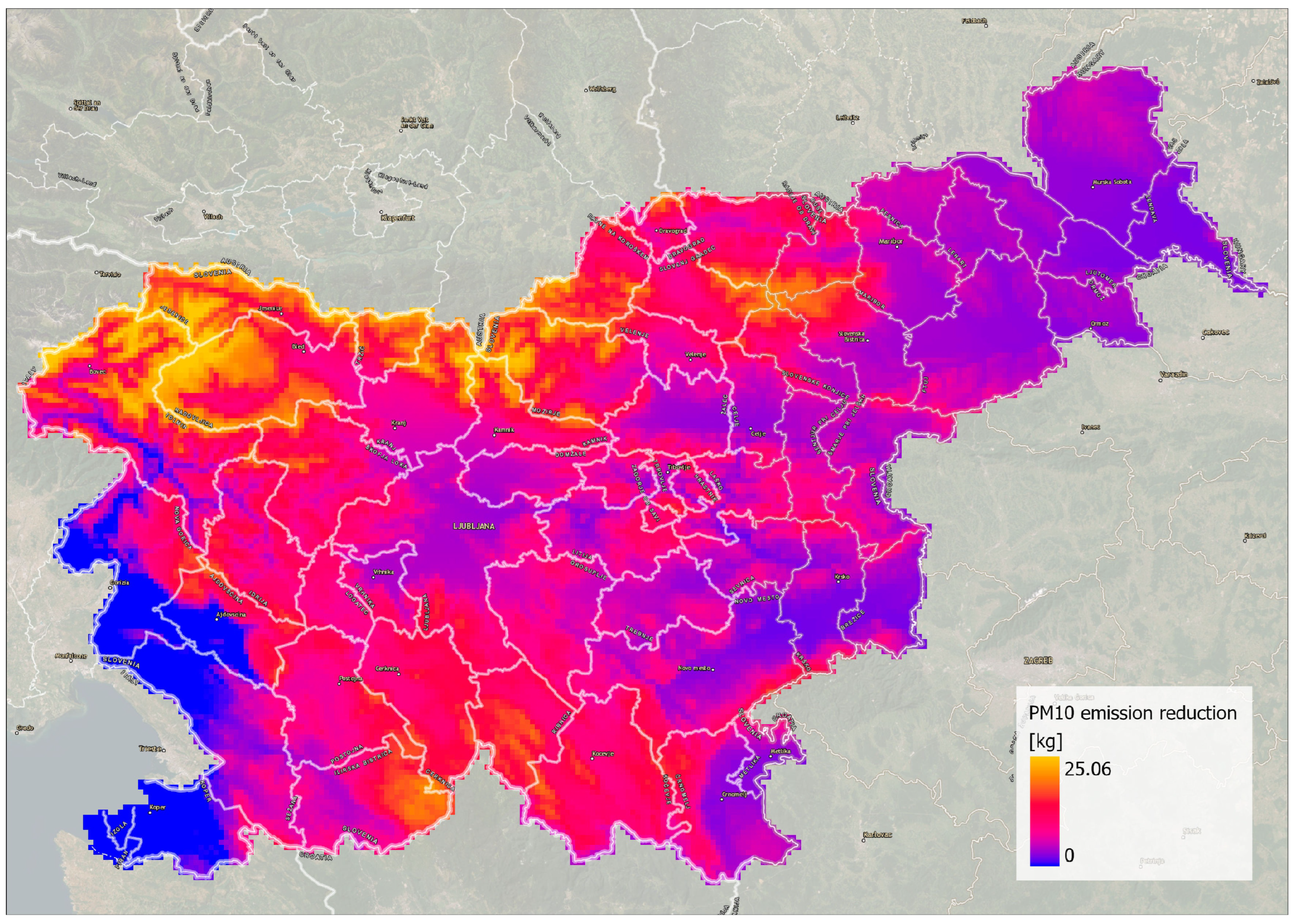
Figure 9 displays the spatial distribution of yearly PM₁₀ emission reduction per single-family building resulting from the bivalent operation of a HHP compared to monovalent heating with a biomass boiler. The data covers the area of Slovenia at a spatial resolution of 1 km × 1 km. In the south-western coastal area, a PM₁₀ emission reduction of 0 kg is proposed, as the bivalent operation of HHP systems is not economically feasible under these climatic conditions.

The greatest reductions, reaching up to 25 kg, are observed in the yellow-coloured areas corresponding to the Alpine mountain regions and peaks, which are largely unpopulated. However, in populated Alpine valleys and the Dinaric plateaus, where heating degree days vary between 4000 K day and 5500 K day, the bivalent operation of the HHP can reduce PM₁₀ emissions by 15–20 kg. Most populated areas in Slovenia are cities located in lowland basins with a milder climate, where heating degree days range from 2500 K day to 3000 K day, and the bivalent operation of the HHP can still reduce emissions by more than 10 kg. However, energy infrastructure in cities is more developed and diverse, making district heating or natural gas more convenient. In contrast, the spatial analysis shows that in rural areas in the south and west, as well as in the northern Alpine valleys, where biomass is a reliable local heating source, yearly PM₁₀ emissions can be reduced by up to 15 kg for one single-family building.

Compared with previous studies, which have predominantly focused on gas-assisted hybrid heat pumps and optimised energy use, operating costs, and GHG emissions, the present model provides a more comprehensive assessment by simultaneously considering temperature-dependent ASHP performance, building heat-loss characteristics, capacity-based electricity tariffs, time-dependent electricity carbon intensity, and PM₁₀ emissions from biomass combustion. Its validation against measured electricity consumption and application across a wide range of climatic and building conditions further strengthen its practical relevance. Although the current rule-based approach is less flexible than model predictive control, its relatively low computational complexity and transparent optimisation of the switching temperature make it suitable for adaptation to in loco operational optimisation. Coupled with measured building data and short-term weather, tariff, carbon-intensity, and potentially air-quality forecasts, the model could dynamically optimise heat pump and biomass boiler operation according to economic, grid, or environmental objectives.

4. Conclusions

In this study, the economic and environmental performance of a bivalent ASHP–biomass boiler system was evaluated for the retrofit of existing single-family buildings equipped with biomass boilers. A model was developed to determine the cost-optimal cut-off temperature while accounting for a new electricity distribution cost methodology. The analysis covered 23 locations across Slovenia and different building heat-loss characteristics, enabling the influence of climatic conditions and building demand to be assessed. The proposed methodology is intended as a general framework for evaluating the feasibility of hybrid heat pump systems rather than for detailed modelling of a specific building. It can be applied using hourly climatic data and different total heat loss coefficients, and can therefore support assessments across various building types, sizes, and climatic regions.

Compared with a monovalent ASHP, bivalent operation can reduce operating costs by up to approximately 10%, while GHG emission reductions can exceed 30% under colder climatic conditions. Compared with monovalent biomass heating, operating cost reductions of up to approximately 15% for insulated buildings and 25% for uninsulated buildings were obtained, while annual PM₁₀ emissions can typically be reduced by 4–7 kg and 15–21 kg per building, respectively. The spatial analysis indicates the greatest practical potential in colder rural areas and Alpine valleys, where reductions of approximately 15–20 kg in PM₁₀ per building and year can be achieved. These findings show that retaining an existing biomass boiler as an auxiliary heat source can facilitate heat pump deployment while reducing operating costs, limiting peak electricity demand, and substantially decreasing local particulate emissions.

The proposed approach extends previous assessments of hybrid heat pumps by jointly considering operating costs, grid-related tariffs, time-dependent GHG emissions, and local PM₁₀ emissions across different climatic conditions and building heat-loss characteristics. The present control strategy is optimised with respect to annual operating costs, while GHG and PM₁₀ emissions are evaluated as resulting performance indicators. Consequently, the cost-optimal switching temperature does not necessarily represent the environmentally optimal operating point, particularly during winter temperature inversions when reduced atmospheric dispersion can increase local PM₁₀ concentrations. Future work should therefore investigate multi-objective and predictive control strategies that consider operating costs, peak electricity demand, GHG emissions, and PM₁₀ emissions simultaneously and could prioritise ASHP operation during periods of unfavourable air-quality conditions. Pilot-scale validation should additionally account for transient biomass boiler operation and associated emissions.

References

1. Statistični urad Republike Slovenije. Energetika. Available online: https://pxweb.stat.si/SiStat/sl/Podrocja/Index/186/energetika. (accessed on 17 June 2026).
2. Communication from the Commission to the European Parliament, the Council, the European Economic and Social Committee and the Committee of the Regions Securing Our Future Europe’s 2040 Climate Target and Path to Climate Neutrality by 2050 Building a Sustainable, Just and Prosperous Society; Technical Report; European Commission: Strasbourg, France, 2024.
3. Brudermueller, T.; Potthoff, U.; Fleisch, E.; Wortmann, F.; Staake, T. Estimation of energy efficiency of heat pumps in residential buildings using real operation data. Nat. Commun. 2025, 16, 2834. [Google Scholar] [CrossRef] [Scilit] [PubMed]
4. Kamel, R.S.; Fung, A.S.; Dash, P.R. Solar systems and their integration with heat pumps: A review. Energy Build. 2015, 87, 395–412. [Google Scholar] [CrossRef] [Scilit]
5. Namdar, H.; Rossi di Schio, E.; Semprini, G.; Valdiserri, P. Photovoltaic-thermal solar-assisted heat pump systems for building applications: A technical review on direct expansion systems. Energy Build. 2025, 334, 115516. [Google Scholar] [CrossRef] [Scilit]
6. Soleimani, A.; Davidsson, P.; Malekian, R.; Spalazzese, R. Multi-Criteria Model Predictive Controller for Hybrid Heating Systems in Buildings. Energies 2025, 18, 5839. [Google Scholar] [CrossRef] [Scilit]
7. Uche, J.; Tajik Jamalabad, M.; Martínez, A. Configurational Design of a Hybrid System Based on an Air–Water Heat Pump and Biomass Boiler for a Rural Dwelling. Appl. Sci. 2024, 14, 9840. [Google Scholar] [CrossRef] [Scilit]
8. Smillie, S.; Vaishnav, P.; Wade, C.; Jordan, K.; Venkatesh, A.; Sinha, A.; Apt, J. Hybrid heat pumps avoid extreme marginal abatement costs of electrifying peak heating loads in cold regions. Environ. Res. Lett. 2024, 19, 094054. [Google Scholar] [CrossRef] [Scilit]
9. Stafford, A. An exploration of load-shifting potential in real in-situ heat-pump/gas-boiler hybrid systems. Build. Serv. Eng. Res. Technol. 2017, 38, 450–460. [Google Scholar] [CrossRef] [Scilit]
10. Meier, C.; Wemhoener, C. Dual-Source Heat Pump Application for Boiler Replacement—Investigation by Simulation and Field Monitoring. Energies 2025, 18, 5696. [Google Scholar] [CrossRef] [Scilit]
11. Klein, K.; Huchtemann, K.; Müller, D. Numerical study on hybrid heat pump systems in existing buildings. Energy Build. 2014, 69, 193–201. [Google Scholar] [CrossRef] [Scilit]
12. Bonomolo, M.; Leone, G.; Coga, A.; Guarino, S.; Testasecca, T.; Beccali, M. Assessment of Performance of Hybrid Heat Pump System During Winter Season in Different Climatic Conditions. In Proceedings of the 2024 IEEE International Conference on Environment and Electrical Engineering and 2024 IEEE Industrial and Commercial Power Systems Europe (EEEIC/I&CPS Europe), Rome, Italy, 17–20 June 2024; pp. 1–6. [Google Scholar] [CrossRef] [Scilit]
13. Tihana, J.; Ali, H.; Apse, J.; Jekabsons, J.; Ivancovs, D.; Gaujena, B.; Dedov, A. Hybrid Heat Pump Performance Evaluation in Different Operation Modes for Single-Family House. Energies 2023, 16, 7018. [Google Scholar] [CrossRef] [Scilit]
14. Di Perna, C.; Magri, G.; Giuliani, G.; Serenelli, G. Experimental assessment and dynamic analysis of a hybrid generator composed of an air source heat pump coupled with a condensing gas boiler in a residential building. Appl. Therm. Eng. 2015, 76, 86–97. [Google Scholar] [CrossRef] [Scilit]
15. Saffari, M.; Keogh, D.; De Rosa, M.; Finn, D.P. Technical and economic assessment of a hybrid heat pump system as an energy retrofit measure in a residential building. Energy Build. 2023, 295, 113256. [Google Scholar] [CrossRef] [Scilit]
16. Buday, T.; Buday-Bódi, E. Reduction in CO2 Emissions with Bivalent Heat Pump Systems. Energies 2023, 16, 3209. [Google Scholar] [CrossRef] [Scilit]
17. Biéron, M.; Le Dréau, J.; Haas, B. Development of a GHG-based control strategy for a fleet of hybrid heat pumps to decarbonize space heating and domestic hot water. Appl. Energy 2025, 378, 124751. [Google Scholar] [CrossRef] [Scilit]
18. Silva, D.D.; Jean-Baptiste, V.; Trentin, P.; Rached, G.A.; Muresan, C. Study of Hybrid Heat Pump Flexibility Potential Applied to French Building Stock. 2024. Available online: https://www.researchgate.net/publication/380733938_Study_of_hybrid_heat_pump_flexibility_potential_applied_to_French_building_stock (accessed on 8 March 2025).
19. Simic, K.; Scheirlinckx, A.; Faes, W.; De Paepe, M. Commissioning and numerical performance assessment of a hybrid heat pump system for an office building. In Proceedings of the ECOS 2022—The 35th International Conference on Efficiency, Cost, Optimization, Simulation and Environmental Impact of Energy Systems, Copenhagen, Denmark, 3–7 July 2022; pp. 1560–1570. [Google Scholar] [CrossRef]
20. Schito, E.; Conti, P.; Testi, D.; Montagud-Montalvá, C.; Vivancos, J.L. Economic and environmental assessment of hybrid heat pumps: A cross-country analysis. Energy Build. 2026, 353, 116857. [Google Scholar] [CrossRef] [Scilit]
21. Beccali, M.; Bonomolo, M.; Martorana, F.; Catrini, P.; Buscemi, A. Electrical hybrid heat pumps assisted by natural gas boilers: A review. Appl. Energy 2022, 322, 119466. [Google Scholar] [CrossRef] [Scilit]
22. Bizzarri, M.; Conti, P.; Schito, E.; Testi, D. Improving energy efficiency through forecast-driven control in hybrid heat pumps. Energy Convers. Manag. 2025, 332, 119737. [Google Scholar] [CrossRef] [Scilit]
23. Lin, H.; Clavreul, J.; Jeandaux, C.; Crawley, J.; Butnar, I. Environmental life cycle assessment of heating systems in the UK: Comparative assessment of hybrid heat pumps vs. condensing gas boilers. Energy Build. 2021, 240, 110865. [Google Scholar] [CrossRef] [Scilit]
24. Biéron, M.; Dréau, J.L.; Haas, B. Assessment of the marginal technologies reacting to demand response events: A French case-study. Energy 2023, 275, 127415. [Google Scholar] [CrossRef] [Scilit]
25. Uche, J.; Jamal-Abad, M.T.; Martínez-Gracia, A. Evaluating the efficiency, economics, and environmental impact of hybrid heat pumps assisted by biomass boilers for Spanish climate zones. Energy 2025, 325, 136180. [Google Scholar] [CrossRef] [Scilit]
26. Katerla, J.; Sornek, K. Biomass for Residential Heating: A Review of Technologies, Applications, and Sustainability Aspects. Energies 2025, 18, 5875. [Google Scholar] [CrossRef] [Scilit]
27. Wüllhorst, F.; Schwarz, S.; Fuchs, N.; Maier, L.; Monti, A.; Müller, D. Impact of hybrid heat pump shares and building envelope retrofit rates on load penetration in German low-voltage grids. Appl. Energy 2025, 388, 125530. [Google Scholar] [CrossRef] [Scilit]
28. Cholewa, T.; Bejan, A.S.; Miara, M.; Schauer, C.; Kosonen, R.; Borodiņecs, A.; Bogdanovičs, R.; Amanowicz, Ł.; Vering, C.; Siuta-Olcha, A.; et al. Critical discussion on the challenges of integrating heat pumps in hydronic systems in existing buildings. Energy 2025, 326, 136158. [Google Scholar] [CrossRef] [Scilit]
29. Glojek, K.; Gregorič, A.; Močnik, G.; Cuesta-Mosquera, A.; Wiedensohler, A.; Drinovec, L.; Ogrin, M. Hidden black carbon air pollution in hilly rural areas. A case study of dinaric depression. Eur. J. Geogr. 2020, 11, 105–122. [Google Scholar] [CrossRef] [Scilit]
30. Kocbach Bølling, A.; Pagels, J.; Yttri, K.E.; Barregard, L.; Sallsten, G.; Schwarze, P.E.; Boman, C. Health effects of residential wood smoke particles: The importance of combustion conditions and physicochemical particle properties. Part. Fibre Toxicol. 2009, 6, 29. [Google Scholar] [CrossRef] [Scilit] [PubMed]
31. Roccatello, E.; Prada, A.; Baggio, P.; Baratieri, M. Analysis of the Influence of Control Strategy and Heating Loads on the Performance of Hybrid Heat Pump Systems for Residential Buildings. Energies 2022, 15, 732. [Google Scholar] [CrossRef] [Scilit]
32. Stegnar, G. Strategic Prioritization of Residential Buildings for Equitable and Sustainable Renovation. Sustainability 2025, 17, 2203. [Google Scholar] [CrossRef] [Scilit]
33. Hoops, H.; Tjaden, T.; Rösken, K. RE-Lab-Projects/hplib: v1.9. 2022. Available online: https://zenodo.org/records/6792486 (accessed on 4 July 2025). [CrossRef]
34. Carlon, E.; Schwarz, M.; Golicza, L.; Verma, V.K.; Prada, A.; Baratieri, M.; Haslinger, W.; Schmidl, C. Efficiency and operational behaviour of small-scale pellet boilers installed in residential buildings. Appl. Energy 2015, 155, 854–865. [Google Scholar] [CrossRef] [Scilit]
35. Heat Pump KEYMARK Certificates. Available online: https://keymark.eu/en/products/heatpumps/certified-products (accessed on 19 March 2025).
36. Schwamberger, K. Modellbildung und Regelung von Gebäudeheizungsanlagen mit Wärmepumpen; VDI-Verlag: Düsseldorf, Germany, 1991. [Google Scholar]
37. Slovenian Environment Agency. Typical Reference Year. Available online: https://meteo.arso.gov.si/met/sl/climate/tables/test_ref_year/ (accessed on 19 March 2025).
38. VDI. Thermal Use of the Underground: Ground Source Heat Pump Systems; Richtlinien VDI 4640, Blatt 2; VDI: Düsseldorf, Germany, 2001. [Google Scholar]
39. Electricity Maps. Slovenia|Datasets|Electricity Maps. 2025. Available online: https://portal.electricitymaps.com/datasets/SI (accessed on 19 March 2025).
40. Slovenian Energy Agency. Akt o Metodologiji za Obračunavanje Omrežnine za Elektrooperaterje. 2022. Available online: https://pisrs.si/pregledPredpisa?id=AKT_1266 (accessed on 8 August 2024).
41. Kopač, J. Increasing the Capacity of the Distribution Network by Changing Consumers’ Habits—Case Study. B&H Electr. Eng. 2023, 17, 21–25. [Google Scholar] [CrossRef] [Scilit]
42. Tarifne Postavke—URO. Available online: https://www.uro.si/prenova-omre%C5%BEnine/tarifne-postavke (accessed on 12 August 2024).
43. Cene Lesnih Goriv. Available online: https://wcm.gozdis.si/sl/podatki/cene/podatki/2021100415210921/cene-lesnih-goriv/ (accessed on 1 July 2025).
44. Vicente, E.D.; Vicente, A.M.; Evtyugina, M.; Tarelho, L.A.; Almeida, S.M.; Alves, C. Emissions from residential combustion of certified and uncertified pellets. Renew. Energy 2020, 161, 1059–1071. [Google Scholar] [CrossRef] [Scilit]
45. Stegnar, G.; Šijanec Zavrl, M.; Stankovski, V. The use of information sources for typification of buildings in Slovenia. Gradb. Vestn. 2012, 61, 256–262. [Google Scholar]
46. Ogrin, D.; Repe, B.; Štaut, L.; Svetlin, D.; Ogrin, M. Podnebna tipizacija Slovenije po podatkih za obdobje 1991–2020. Dela 2023, 59, 5–89. [Google Scholar] [CrossRef] [Scilit]
Figure 1. Heating system operation: monovalent (a), bivalent alternate (b), and bivalent parallel operation (c).
Energies 19 04216 g001
Figure 2. Characteristics of a regulated air-source heat pump and thermal losses of a building. Simulated data are from the hplib library [33].
Energies 19 04216 g002
Figure 3. Flow chart of a model for relative cost, GHG, and PM10 emission simulation.
Energies 19 04216 g003
Figure 4. Daily distribution of time slots for working and non-working days in the high and low seasons.
Energies 19 04216 g004
Figure 5. Comparison between yearly modelled electricity consumption and measured consumption in 2024.
Energies 19 04216 g005
Figure 6. Relative energy costs and GHG emissions of HHP compared to monovalent ASHP and relative PM10 emissions compared to monovalent biomass boiler.
Energies 19 04216 g006
Figure 7. Relative cost and GHG emission reduction of bivalent heating compared to a monovalent ASHP for an uninsulated (left) and an insulated (right) single-family building.
Energies 19 04216 g007
Figure 8. Relative cost and absolute PM10 emission reduction of bivalent heating compared to a monovalent biomass boiler for an uninsulated (left) and an insulated (right) single-family building.
Energies 19 04216 g008
Figure 9. Yearly PM10 emission reduction for the bivalent operation of the HHP compared to a monovalent biomass boiler for a single-family building in economically viable scenarios.
Energies 19 04216 g009