Effect of Operating Void Fraction on Wall-Deposited Decay Heat in the Main Loop of a Molten Salt Reactor

Abstract

In molten salt reactors, multiphase transport of fission products produces nonuniform nuclide inventories throughout the primary loop, thereby affecting subsequent decay heat evolution. Although fission product transport has been widely studied, its influence on post-shutdown wall-deposited decay heat remains insufficiently characterized. Here, the bubble transport capability of the Thorium Fission Products Migration Code (ThorFPMC) was extended using a drift-flux model to investigate the effects of operating void fraction on the magnitude, spatial distribution, nuclide composition, and subsequent evolution of wall-deposited decay heat under an idealized post-drainage condition. Results showed that, for the baseline bubble diameter of 0.508 mm, the initial wall-deposited decay heat decreased from 41.33 to 6.63 kW as the operating void fraction increased, corresponding to an 84.0% reduction; bubble diameter sensitivity calculations preserved the same monotonic trend. The source remained strongly nonuniform, with the heat exchanger consistently dominant, while increasing the void fraction reduced the core fraction and increased the relative external-loop contribution. Nuclide contributions evolved from a broad early distribution to long-term dominance by ⁹⁵Nb and ¹⁰³Ru, with precursor feeding shaping several important daughter nuclides. These results link operating period multiphase transport to component-resolved residual decay heat sources and provide a basis for operating-condition-dependent source terms in shutdown thermal and system analyses.

1. Introduction

The circulating liquid fuel distinguishes molten salt reactors from conventional solid-fueled systems. As the fuel salt flows through the core and external primary loop, fission products can be redistributed from their locations of production by bulk flow, interphase mass transfer, surface deposition, and removal [1]. Because the decay heat at a given location depends on the local nuclide inventory and composition, these transport processes make the decay heat source spatially distributed and dependent on the preceding operating history [2]. Decay heat assessment in molten salt reactors therefore requires consideration of fission product transport and the resulting redistribution of nuclide inventories throughout the primary system.

Experiments conducted during the Molten Salt Reactor Experiment (MSRE) provided an early basis for understanding fission product migration and retention in circulating fuel salt, particularly the transport and deposition of insoluble noble metal species among the salt, structural surfaces, graphite, and gas–liquid interfaces [3,4]. Subsequent studies examined the formation, growth, transport, deposition, and removal of insoluble particles [1,5,6,7,8], as well as gaseous fission product behavior, xenon control, off-gas removal, and bubble-assisted transport [9,10,11,12,13]. At the system scale, these processes are commonly represented using reduced-order models for mass transfer, deposition, and removal, whereas higher-fidelity computational fluid dynamics, particle tracking, and population balance methods resolve local flow, particle size, and interfacial effects in greater detail [14,15]. Decay heat analysis has likewise advanced from early MSRE safety calculations based on point-depletion estimates [16] to flow-depletion analyses [2,17,18,19,20] and coupled flow–transfer–depletion calculations [21] that resolve the spatial and temporal evolution of decay heat. However, the post-shutdown decay heat generated by inventories retained on individual components has received limited quantitative attention [21], and the dependence of this heat source on operating period multiphase transport remains poorly characterized.

This operating condition dependence is particularly relevant to shutdown scenarios involving fuel salt transfer or drainage. During power operation, fission power dominates the total heat generation, and the decay heat produced by surface-deposited inventories represents only a small part of the system heat load. After shutdown, however, the fission source is terminated, and radioactive decay becomes the principal residual heat source. Mobile nuclide inventories may be removed with the fuel salt, whereas insoluble fission products deposited on primary-loop surfaces may remain on their original components. Their subsequent decay forms a persistent, spatially fixed, component-associated heat source. This source may become particularly important after the mobile fuel salt inventory is removed, and its magnitude, distribution, and nuclide composition are established during reactor operation. Because circulating gas bubbles provide an interfacial transport pathway that competes with wall deposition, the operating void fraction may affect the total wall-deposited inventory at shutdown, its component-level distribution, and its nuclide composition. The central question is therefore how the operating void fraction affects the magnitude, spatial distribution, nuclide composition, and post-shutdown evolution of the wall-deposited decay heat source.

To address this question, the present study uses a coupled multiphase fission product transport and nuclide evolution framework to quantify how the operating void fraction affects the wall-deposited inventory at shutdown. A shutdown initial condition is then constructed by retaining only the wall-associated inventories in the primary-system components, after which the residual source evolves through radioactive decay and daughter nuclide ingrowth only. The resulting wall-deposited decay heat source is evaluated in terms of total magnitude, component-level distribution, temporal evolution, nuclide composition, decay chain evolution, and precursor contributions. By linking operating period multiphase transport to post-shutdown wall-deposited decay heat, this study quantifies the relationship between the operating void fraction and the component-resolved decay heat source retained in the primary loop.

The remainder of this paper is organized as follows. Section 2 presents the multiphase fission product transport and nuclide evolution framework, the MSRE nodal model and bubble field treatment, the numerical implementation and model assessment, and the operating and post-shutdown analysis conditions. Section 3 reports the effects of the operating void fraction on the magnitude, spatial distribution, and temporal evolution of wall-deposited decay heat, and further interprets the nuclide-specific responses, decay chain family evolution, and precursor contributions, together with their implications for shutdown decay heat representation. Section 4 summarizes the principal conclusions and outlines directions for future work.

2. Model and Methodology

The overall analysis consists of two sequential stages. During reactor operation, the Thorium Fission Products Migration Code (ThorFPMC) is used to determine the spatial and phase-associated nuclide inventories established under different operating void fractions. At shutdown, the wall-associated inventories are isolated as the residual source under an idealized post-drainage condition and subsequently evolved through radioactive decay and daughter nuclide ingrowth only. Accordingly, Section 2.1 describes the physical transport model and spatial representation, Section 2.2 summarizes the numerical implementation and model assessment, and Section 2.3 defines the operating cases, shutdown source construction, and analysis methods used in this study.

2.1. Physical Model and Spatial Discretization

2.1.1. Multiphase Fission Product Transport Framework

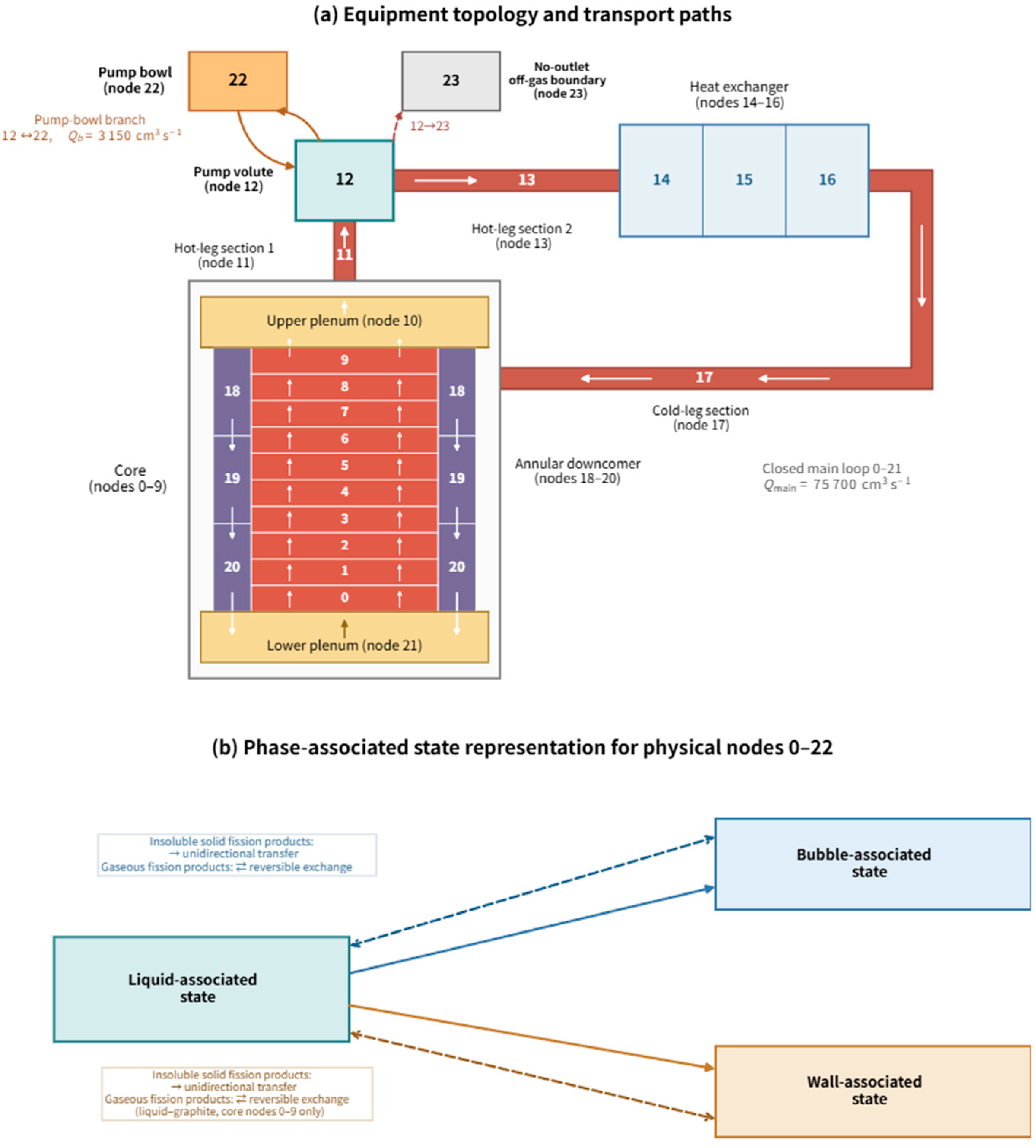
Fission product evolution in the circulating-fuel molten salt reactor was represented using a unified multiphase framework in which nuclide inventories were tracked in liquid-, bubble-, and wall-associated states. During reactor operation, fission product generation and nuclide transformation occurred concurrently with inter-node transport, interphase mass transfer, wall deposition, and inventory transfer from the pump region to a no-outlet off-gas accumulation boundary. Insoluble solid fission products were transferred from the liquid-associated state to bubbles and component surfaces, whereas gaseous fission products exchanged reversibly between the fuel salt and bubbles throughout the primary loop and between the fuel salt and graphite within the core. Gaseous inventories retained in graphite were included in the wall-associated state of the corresponding core node. In this study, wall-deposited inventory is used as an aggregate term for all inventories retained in the wall-associated state, including insoluble species deposited on component surfaces and gaseous species retained in core graphite. This terminology defines the statistical boundary of the shutdown source term and does not imply that solid deposition and gaseous retention follow the same transfer mechanism. For the post-shutdown calculations, all physical transport and transfer processes were deactivated. Fission product generation and neutron-induced reactions were also terminated, leaving only radioactive decay and daughter nuclide ingrowth.

The nuclide concentrations in all physical nodes and phase-associated states were assembled into a unified state vector, c, whose evolution was governed by:

$$\begin{array}{cccc} & {\displaystyle \frac{dc}{dt}}=\left(A_B+A_M+A_F+A_R\right)c+f=Ac+f.& & \end{array}$$

(1)

The depletion matrix $A_B$ accounts for fission product generation, radioactive decay and daughter nuclide production, and neutron-induced reactions. The mass-transfer matrix $A_M$ represents transfers among phase-associated inventories within the same physical node, whereas the flow matrix $A_F$ describes the inter-node transport of liquid- and bubble-associated inventories according to the prescribed network flow representation. The transfer/removal matrix $A_R$ represents the prescribed inventory transfers associated with the pump region, pump bowl branch, and off-gas pathway. Transfer to the off-gas node denotes redistribution from the circulating primary loop to the no-outlet off-gas accumulation boundary rather than loss from the entire modeled system. The vector $f$ denotes the external feed term and was set to zero in all calculations. For each operating case, the temperature, pressure, flow, and bubble field parameters were prescribed as fixed inputs; therefore, the coupled evolution matrix A was time-invariant during the calculation.

Within each physical node, the interphase mass-transfer rate was expressed as the product of the local mass-transfer coefficient, interfacial area, and concentration driving force [3]:

$$\begin{array}{cccc} & J_{i,k}=h_k{A}_k\mathsf{\Delta }{c}_{i,k}.& & \end{array}$$

(2)

Here, $J_{i,k}$ denotes the net transfer rate of nuclide $i$ in node $k$, and $h_k$, $A_k$, and $\mathsf{\Delta }{c}_{i,k}$ denote the corresponding mass-transfer coefficient, interfacial area, and concentration driving force, respectively. For insoluble solid fission products, transfer from the liquid-associated state to the bubble- and wall-associated states was treated as unidirectional, with no detachment or reverse transfer of the deposited species. Gaseous fission products underwent reversible exchange between the fuel salt and bubbles throughout the primary loop and between the fuel salt and graphite within the core. For liquid–gas exchange, the net transfer rate was determined from the deviation from Henry’s law equilibrium [10]:

$$\begin{array}{cccc} & J_{i,k}^{l\leftrightarrow g}=h_k{A}_k\left(c_{i,k}^l-H_{i}R{T}_k{c}_{i,k}^g\right).& & \end{array}$$

(3)

Superscripts $l$ and $g$ denote the liquid and gas phases, respectively. The sign of the concentration driving force determined the transfer direction. The same equilibrium-based formulation was used for fuel salt–graphite exchange in the core, with the corresponding mass-transfer coefficient, interfacial area, and equilibrium parameter. If radioactive decay or neutron-induced reactions changed the nuclide identity and physicochemical classification, the resulting inventory was reassigned to the liquid-, bubble-, or wall-associated state according to the classification of the product nuclide. This reassignment resulted from nuclide transformation rather than physical detachment or reverse transfer of the original species. As the bubble-associated transfer terms depend on the local gas holdup and interfacial area, the node-dependent bubble field required by the transport framework was determined separately, as described below.

2.1.2. Bubble Transport Model

The required node-dependent bubble parameters were generated offline using a drift-flux model and supplied one way to ThorFPMC as fixed inputs for each operating case. For each void fraction case, the prescribed void fraction at node 0 was first used to determine the gas flow rate. The gas flow rate was then conserved through serial sections and partitioned at branches according to the prescribed flow distribution. Consequently, the local gas superficial velocity, $u_{g,k}^{sup}$, was known before the local void fraction was evaluated. The local void fraction in node $k$ was calculated using the drift-flux relation [22]:

$$\begin{array}{cccc} & {\alpha }_k={\displaystyle \frac{u_{g,k}^{sup}}{C_0(u_{l,k}^{sup}+u_{g,k}^{sup})+s_k{u}_d}}.& & \end{array}$$

(4)

Here, $u_{g,k}^{sup}$ and $u_{l,k}^{sup}$ denote the gas and liquid superficial velocities, respectively, and $C_0=1.2$ is the distribution parameter [23]. The orientation factor $s_k$ was set to $+1$, $0$, or $-1$ when the buoyant drift was aligned with the main flow, had no axial projection, or was opposed to the main flow, respectively. The drift velocity was calculated as [24]:

$$\begin{array}{cccc} & u_d=1.53{\left[{\displaystyle \frac{\sigma g\left({\rho }_l-{\rho }_g\right)}{{\rho }_l^2}}\right]}^{1/4}.& & \end{array}$$

(5)

where $\sigma$, $g$, ${\rho }_l$, and ${\rho }_g$ denote the surface tension, gravitational acceleration, liquid density, and gas density, respectively.

Assuming monodisperse spherical bubbles, the node-dependent bubble diameter was corrected for local temperature and pressure using the ideal-gas expansion relation:

$$\begin{array}{cccc} & d_{b,k}=d_{b,0}{\left({\displaystyle \frac{T_k}{T_0}}{\displaystyle \frac{P_0}{P_k}}\right)}^{1/3}.& & \end{array}$$

(6)

The bubble volume, gas–liquid interfacial area, and specific interfacial area in node $k$ were then calculated as:

$$\begin{array}{cccc} & V_{b,k}={\alpha }_k{V}_k,A_{b,k}={\displaystyle \frac{6V_{b,k}}{d_{b,k}}},a_{b,k}={\displaystyle \frac{A_{b,k}}{V_k}}={\displaystyle \frac{6{\alpha }_k}{d_{b,k}}}.& & \end{array}$$

(7)

Here, $V_k$ is the total volume of node $k$, and the reference bubble radius and diameter were 0.254 and 0.508 mm, respectively [25]. The bubbles were assumed to be monodisperse and spherical, and bubble coalescence, breakup, and size distribution effects were neglected. The temperature, pressure, liquid flow conditions, and flow orientation parameters were fixed within each operating case. The resulting node-dependent void fraction, bubble size, bubble volume, and interfacial area were then supplied as fixed inputs to the fission product transport calculation for each operating case.

2.1.3. Spatial Discretization

The modeled MSRE system was discretized into 24 computational nodes, comprising 23 physical nodes for the primary system and one no-outlet off-gas accumulation boundary. This representation was used to resolve component- and location-dependent nuclide transport, wall-associated inventories during operation, and the resulting wall-deposited decay heat after shutdown. The nodalization was based on the primary-system topology, component volumes, flow rates, characteristic residence times, and the resolution required to track short-lived nuclides. For distributed components with predominantly axial flow, a nominal residence time of approximately 1 s per node was used as a practical guideline to balance the transport resolution of short-lived nuclides and the model size, rather than as a strict nodalization criterion. Accordingly, the core, heat exchanger, and annular downcomer were subdivided along the flow direction, whereas the upper and lower plena and the pump volute were represented by lumped nodes. Hydraulically distinct pipe sections were retained as separate nodes even when their residence times were shorter than 1 s. The resulting nodal assignments and flow topology are summarized in

Table 1. Component residence times and physical node assignments of MSRE.

Region	Volume (m3)	Residence Time (s)	Node Number
Core region	0.78	10.32	0–9
Upper plenum	0.30	3.93	10
Hot-leg section 1	5.94 × 10−2	0.79	11
Pump volute	2.55 × 10−2	0.34	12
Hot-leg section 2	2.27 × 10−2	0.30	13
Heat exchanger	0.17	2.28	14–16
Cold-leg section	6.23 × 10−2	0.82	17
Annular downcomer	0.27	3.63	18–20
Lower plenum	0.28	3.74	21
Pump bowl	9.06 × 10−2	11.97	22
Off-gas system	—	—	23

and illustrated in Figure 1 [26].

Nodes 0–21 form the closed primary-loop circulation path through the core, upper plenum, hot-leg sections, pump volute, heat exchanger, cold leg, annular downcomer, and lower plenum. Node 22 represents the low-flow pump bowl recirculation branch connected to pump volute node 12. The volumetric flow rates in the closed primary loop and the pump bowl branch were 75,700 and 3150 cm³ s⁻¹, respectively. Physical nodes 0–22 were assigned liquid-, bubble-, and wall-associated states to track the local nuclide inventories. Node 23 represents a no-outlet off-gas accumulation boundary that receives prescribed nuclide inventories transferred from the pump region but does not participate in primary-loop circulation. Transfer to node 23 therefore represents redistribution from the circulating loop to the off-gas boundary rather than removal from the entire modeled system.

2.2. Numerical Implementation and Model Assessment

The numerical implementation and physical consistency of the transport framework were assessed at three complementary levels. First, the numerical solution and code implementation were examined through verification calculations. Second, the drift-flux-based bubble transport treatment was assessed by examining its influence on the node-dependent void fraction and gas–liquid interfacial area. Finally, the calculated noble metal inventory distributions were compared with historical MSRE data to assess the physical consistency of the coupled transport treatment.

2.2.1. Numerical Implementation and Verification

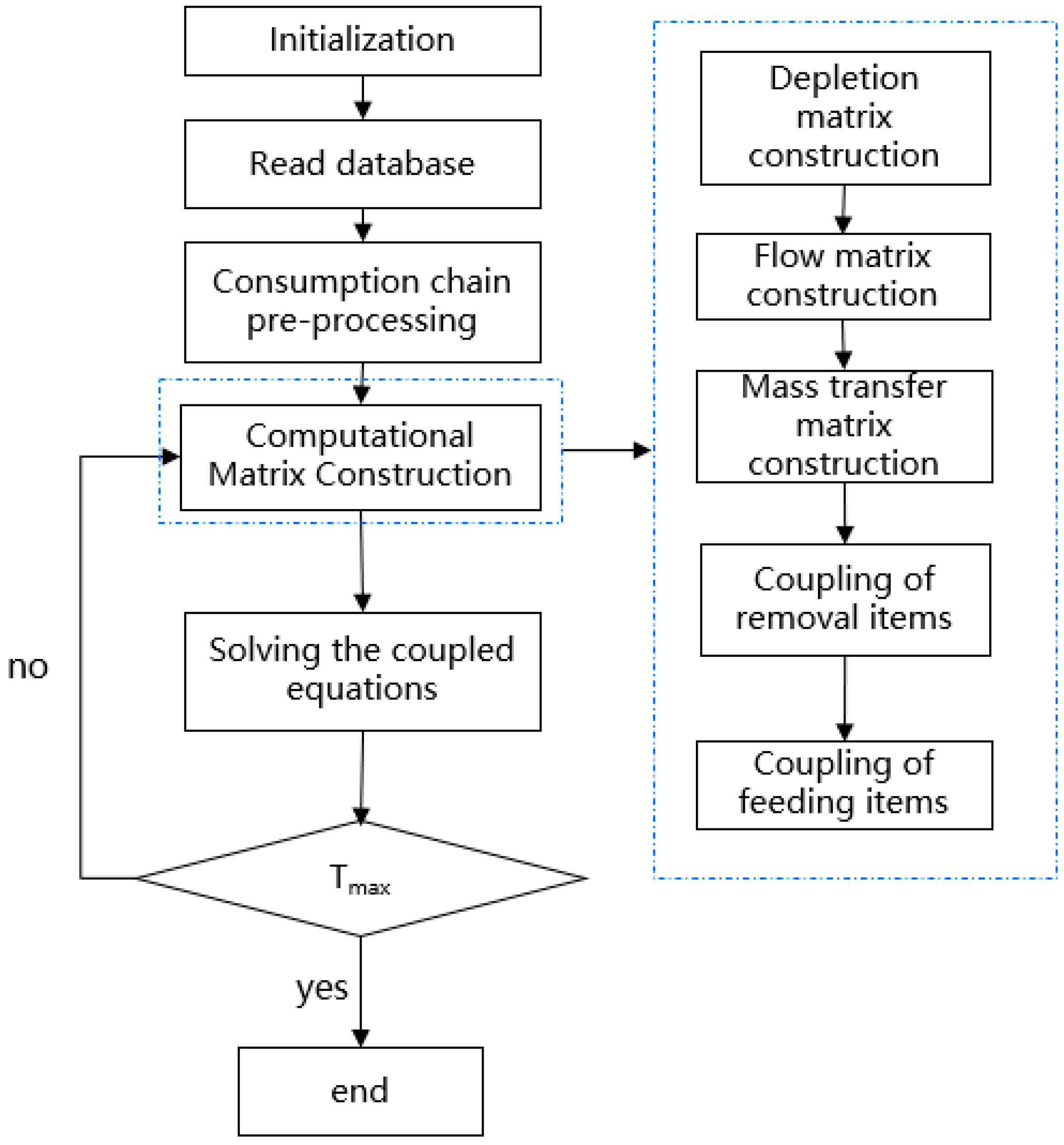
The multiphase fission product transport and nuclide evolution calculations were performed using ThorFPMC, which couples a multiphase network transport model with the Molten Salt Reactor Specific Depletion Code (MODEC) nuclide evolution module [27]. The depletion, inter-node flow, interphase mass transfer, and prescribed transfer/removal terms were assembled into a unified evolution matrix. The resulting coupled equations were solved over the prescribed calculation period following the workflow shown in Figure 2 [28].

The coupled evolution equations were solved using the Chebyshev Rational Approximation Method (CRAM) [29], with the resulting sparse linear systems solved by PARDISO [30]. Previous verification calculations yielded infinity-norm relative errors on the order of ${10}^{-8}$ for the liquid-associated inventories and ${10}^{-4}$ for the bubble- and wall-associated inventories [28]. The nuclide depletion, radioactive decay, and daughter-ingrowth calculations performed by MODEC were also verified in previous work [27]. Relative to the previous model, the 11-node discretization was refined to the present 24-node representation, and the homogeneous bubble treatment was replaced by the drift-flux model described in Section 2.1.2. These changes affected the spatial resolution and local bubble parameters, while the governing nuclide evolution equations and CRAM–PARDISO solution method remained unchanged.

2.2.2. Bubble Transport Model Assessment

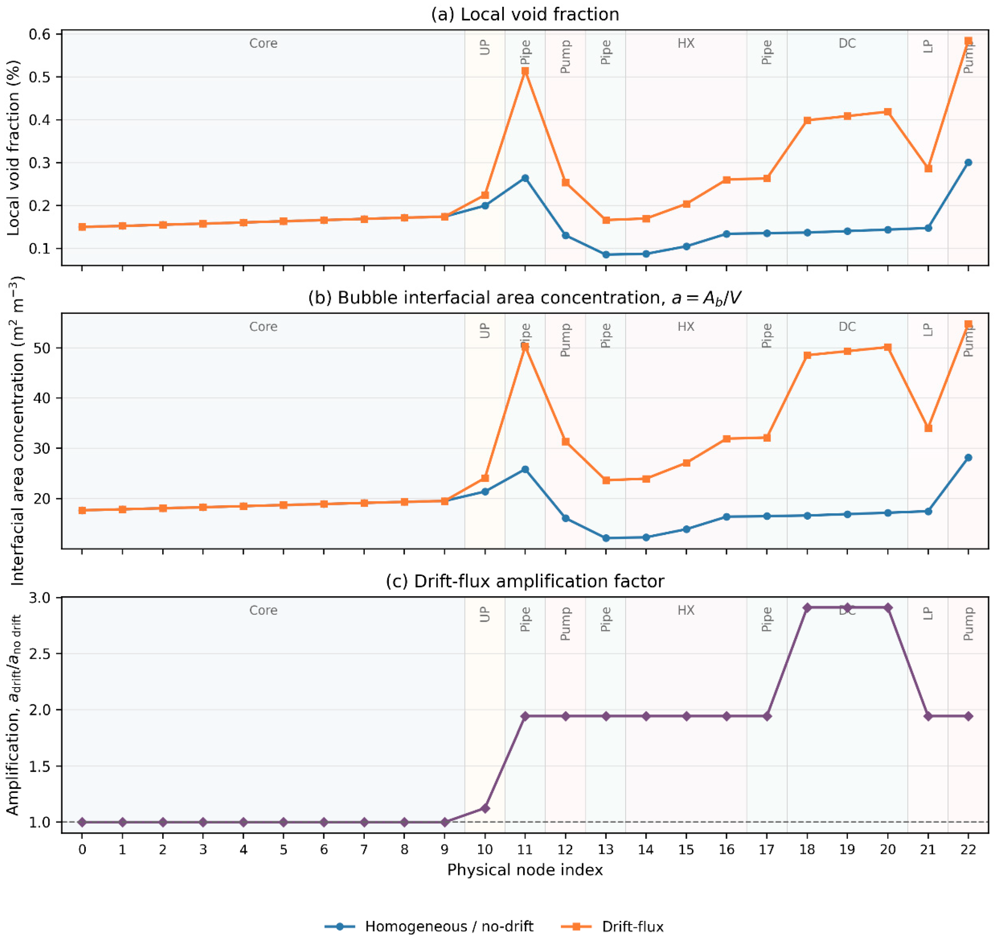
To quantify the effect of gas–liquid slip and flow orientation, the drift-flux model was compared with a homogeneous no-drift model for the representative G3 condition. Both models used the same prescribed void fraction of 0.15% at node 0. The two models used the same temperature- and pressure-dependent bubble size correction and therefore produced identical node-dependent bubble diameters. Differences in the predicted interfacial area arose solely from the spatial redistribution of the local void fraction.

As shown in Figure 3, the two models predicted the same specific interfacial area in core nodes 0–9. The largest difference occurred in the downward-flowing annular downcomer, where the specific interfacial area in nodes 18–20 was 2.911 times that predicted by the homogeneous model. Over physical nodes 0–22, the total gas–liquid interfacial area increased from 37.46 m² under the homogeneous model to 59.64 m² under the drift-flux model, corresponding to an amplification factor of 1.592. Cases G1–G5 exhibited nearly identical normalized amplification patterns.

Under the present dilute-bubble formulation, the prescribed void fraction at node 0 therefore determined the overall scale of the local void fraction and interfacial area, whereas the liquid velocity and flow orientation determined their spatial distribution. This comparison evaluates the effect of the bubble transport model rather than providing experimental validation. It shows that gas–liquid slip and flow orientation can substantially modify the predicted interfacial-area distribution and should therefore be considered when evaluating the competition between bubble capture and wall deposition.

2.2.3. Comparison with MSRE Noble Metal Inventory Distributions

Wall deposition constitutes the principal competing pathway to bubble-mediated transport for insoluble fission products. Because the effective wall-transfer strength depends jointly on the wall mass-transfer coefficient and the available deposition area, the principal component-level wall-transfer parameters used in the present model are summarized in

Table 2. Component-level wall-transfer parameters used in the present transport model.

Component/Region	Node (s)	Effective Wall Area, Aw(m2)	Wall Mass-Transfer Coefficient, hw (m s−1)	Wall Transfer Capacity, (hw·Aw) (m3·s−1)
Core	0–9	136	5.34 × 10−6	7.26 × 10−4
Upper plenum	10	1.30	1.00 × 10−6	1.30 × 10−6
Pump volute	12	2.05	1.04 × 10−4	2.13 × 10−4
Main-loop piping	11,13,17	4.54	1.04 × 10−4	4.62 × 10−4
Heat exchanger	14–16	29.3	4.66 × 10−5	1.37 × 10−3
Annular downcomer	18–20	19.3	4.32 × 10−5	8.34 × 10−4
Lower plenum	21	1.10	1.00 × 10−6	1.10 × 10−6
Pump bowl	22	1.22	2.00 × 10−6	2.44 × 10−6

The relatively low h_w·A_w values adopted for the upper-plenum, lower-plenum, and pump bowl regions result from their effective lumped geometries and account for their comparatively weak but finite wall-transfer contributions.

[3].

To assess the physical consistency of the coupled transport treatment, the calculated noble metal inventory distributions were compared with the historical MSRE inventory assessment reported by Kedl [3] (see

Table 3. Comparison of noble metal inventory distributions with historical MSRE estimates and SPECTRA calculations.

MSRE Runs	Source	Heat Exchanger (%)	Other Hastelloy-N Alloy (%)	Graphite (%)	Pump/Gas/Off-Gas (%)
U-235 runs	MSRE	40.0	50.0	1.0	9.0
	SPECTRA	37.5	47.8	3.9	10.9
	Present model	40.9	49.3	2.2	7.6
U-233 runs	MSRE	6.0	8.0	0.4	86.0
	SPECTRA	4.8	5.9	0.5	88.8
	Present model	6.8	8.2	0.4	84.7

Note: The present model results were regrouped according to the component category convention used in the historical MSRE inventory assessment. Small deviations of published totals from 100% arise from rounding.

). Similar comparisons with MSRE experience have been used in previous noble metal transport studies [3,31]. Because the detailed circulating bubble population in the MSRE was not uniquely characterized, representative low- and high-bubble conditions were considered for the distinct transport regimes observed during the U-235 and U-233 runs. The representative low-bubble condition used a node-0 bubble diameter of 0.500 mm and gas holdup of 0.015%, whereas the high-bubble condition used 0.275 mm and 0.55%, respectively. For consistent comparison, the calculated inventories were regrouped according to the same four component categories used in the historical MSRE inventory assessment.

The present calculations reproduce the major redistribution behavior reported for the two MSRE operating regimes. Under the representative low-bubble condition, 92.36% of the calculated noble metal inventory is associated with the heat exchanger, other Hastelloy-N, and graphite surfaces, compared with approximately 91% in the historical MSRE assessment. Under the representative high-bubble condition, the corresponding wall-associated fraction decreases to 15.26%, while 84.74% is distributed to the pump/gas/off-gas category, compared with approximately 14.4% and 86%, respectively, in the MSRE assessment. The SPECTRA results show the same first-order redistribution between the two regimes. These comparisons demonstrate that the present transport treatment captures the major transition observed in the MSRE from wall-dominated noble metal retention under low-bubble conditions to bubble/off-gas-dominated transport under high-bubble conditions. Remaining differences in individual component fractions may reflect uncertainties in the historical inventory reconstruction, differences in the assumed bubble conditions, and simplifications in the component-level transport representation. Because the historical MSRE data are component-integrated and the detailed bubble population and local transport parameters were not uniquely characterized, this comparison is used to assess the first-order physical consistency of the coupled transport treatment rather than to provide a unique validation of individual node-level parameters.

2.3. Operating Conditions, Shutdown Source Construction, and Analysis Methods

The shutdown decay heat analysis was performed in three sequential steps. First, operating period multiphase transport calculations were used to establish the nuclide inventories corresponding to each prescribed void fraction case. Second, the inventories retained on primary-system components at the end of operation were isolated to define an idealized post-drainage residual source, which was subsequently evolved using radioactive decay and daughter nuclide ingrowth only. Finally, the resulting decay heat source was analyzed in terms of its total magnitude, spatial distribution, nuclide composition, and decay chain contributions.

2.3.1. Operating Conditions and Void Fraction Cases

The nuclide inventories were evolved from t = 0 under a thermal-spectrum, 235U-fueled MSRE reference configuration to establish the pre-shutdown inventories. The fuel salt was LiF–BeF₂–ZrF₄–UF₄ (69–25–5–1 mol%) with a density of 2.3275 g cm⁻³, and the modeled fuel salt volume in physical nodes 0–22 was approximately 2.070 m³. Each case was operated continuously for 200 d at a constant thermal power of 8 MW. Load following, refueling, and external fuel addition were not considered.

The node-dependent temperatures were prescribed from the SPECTRA calculation [31], while the pressures were specified according to the MSRE assessment [32]. The liquid flow conditions were also held constant, with the main-loop and pump bowl branch flow rates given in Section 2.1.3. The neutron flux was normalized to the prescribed power density and remained constant throughout the operating period. Reactor power, fuel composition, loop geometry, flow conditions, and all transport parameters unrelated to the bubble field were identical among G0–G5. The prescribed operating void fraction and the resulting node-dependent bubble parameters were therefore the only controlled differences among the six cases.

The six void fraction cases were selected to represent conditions ranging from wall-dominated to bubble-dominated interfacial transfer, rather than an evenly spaced parametric sweep. The relative strengths of the two pathways were characterized using the whole-loop nominal transfer-capacity ratio:

$${\mathsf{\Pi }}_{b/w}={\displaystyle \frac{{\displaystyle {\sum }_{k=0}^{22}}{h}_{b,k}{A}_{b,k}}{{\displaystyle {\sum }_{k=0}^{22}}{h}_{w,k}{A}_{w,k}}}.$$

(8)

where the numerator and denominator represent the nominal mass-transfer capacities of the bubble and wall interfaces summed over physical nodes 0–22, respectively. The same reference bubble radius was used at node 0 for all gas-containing cases, and the local void fraction, bubble size, and interfacial area were determined using the bubble transport model described in Section 2.1.2. Cases G0–G5 had reference void fractions of 0, 0.015%, 0.050%, 0.150%, 0.500%, and 1.500% at node 0, corresponding to whole-loop nominal transfer-capacity ratios of approximately 0, 0.1, 0.3, 1, 3, and 10, respectively. Accordingly, G0 was the no-bubble reference; G1 and G2 represented wall-dominated conditions with increasing bubble influence; G3 represented approximate parity between the two nominal transfer capacities; and G4 and G5 represented increasingly bubble-dominated conditions.

2.3.2. Shutdown Initial Condition and Decay-Only Evolution

The present shutdown calculation represents an idealized post-drainage condition rather than the finite-duration salt-drainage transient itself. At the end of the operating period, the inventories retained on primary-system components in physical nodes 0–22, including both direct decay heat contributors and their radioactive precursors, were used to define the post-drainage residual source. Mobile inventories carried by the fuel salt and bubbles, together with the accumulated inventory in off-gas node 23, were excluded. Node 23 received no further inventory after shutdown and was excluded from all post-shutdown decay heat statistics. In matrix form, this initialization can be expressed as:

$$\begin{array}{cccc} & N_{\mathrm{s}\mathrm{d}}\left(0\right)=P_w{N}_{\mathrm{o}\mathrm{p}}\left(200\hspace{0.17em}\mathrm{d}\right).& & \end{array}$$

(9)

where $P_w$ is the operator used to extract the component-retained inventories in physical nodes 0–22 from the operating period inventory vector. This initialization was used to isolate the post-shutdown decay heat associated with inventories retained on primary-system components during operation. Actual shutdown transients may involve time-dependent changes in flow rate, temperature, interphase mass transfer, and salt redistribution or drainage. These retained inventories constitute a distinct residual decay heat source and therefore require separate characterization. The present initialization should thus be interpreted as a source decomposition procedure that isolates the wall-deposited contribution, rather than as a direct simulation of a specific shutdown transient or salt-drainage process.

Following shutdown, fission product generation and neutron-induced reactions were deactivated, leaving only radioactive decay and daughter nuclide ingrowth. The retained inventories remained within their original physical nodes, with no inter-node transport, interphase mass transfer, or removal. The post-shutdown evolution of the regional decay heat was therefore determined by the initial magnitude and nuclide composition of the wall-deposited inventories, together with their subsequent decay chain evolution. All post-shutdown results presented in this study, including the corresponding figures, tables, and supplementary datasets, were generated using this decay-only formulation. The shutdown initial state at 0 s and representative output times from 5 s to 30 d were used to characterize the early and longer-term evolution.

2.3.3. Decay Heat Calculation and Comparative Metrics

Based on the residual source and decay-only evolution defined above, the following quantities were used to characterize its magnitude, spatial distribution, and nuclide composition. The decay heat contribution of nuclide $i$ in physical node $k$ at time $t$ was calculated as:

$$\begin{array}{cccc} & Q_{i,k}\left(t\right)={\lambda }_i{N}_{i,k}\left(t\right)E_i,& & \end{array}$$

(10)

where ${\lambda }_i$, $N_{i,k}\left(t\right)$, and $E_i$ denote the decay constant, nuclide inventory at time $t$, and mean recoverable energy per decay, respectively. The energy carried away by neutrinos was excluded from $E_i$, so that only the recoverable decay energy was included in the decay heat calculation. The decay heat of each physical node was obtained by summing the contributions of all nuclides derived from its projected wall-associated initial inventory. The total wall-deposited decay heat was calculated by summing the node-level contributions over physical nodes 0–22, with off-gas node 23 excluded from the statistical boundary. Component- and region-level decay heats were obtained by summing the corresponding physical-node contributions according to the nodal assignments defined in Section 2.1.3.

To compare the normalized spatial distributions among cases with different total decay heat magnitudes, the decay heat fraction of region $r$ was defined as:

$$\begin{array}{cccc} & f_r\left({\alpha }_m,t\right)={\displaystyle \frac{Q_r\left({\alpha }_m,t\right)}{Q_{\mathrm{l}\mathrm{o}\mathrm{o}\mathrm{p}}\left({\alpha }_m,t\right)}}.& & \end{array}$$

(11)

The post-shutdown evolution of each region was characterized using the normalized remaining fraction:

$$\begin{array}{cccc} & F_r\left({\alpha }_m,t\right)={\displaystyle \frac{Q_r\left({\alpha }_m,t\right)}{Q_r\left({\alpha }_m,0\right)}}.& & \end{array}$$

(12)

where $Q_r\left({\alpha }_m,0\right)$ is the decay heat of region $r$ at shutdown. The degree to which the decay heat contribution was concentrated among a limited number of nuclides was characterized using the cumulative-contribution metric $N_x$. For each case and time, all nuclides were ranked in descending order of their decay heat contributions $Q_{\left(j\right)}$. The metric was defined as the minimum number of ranked nuclides required to account for a cumulative fraction of the total decay heat:

$$\begin{array}{cccc} & N_x=\min \left\{n:{\displaystyle \frac{{\displaystyle {\sum }_{j=1}^n}{Q}_{\left(j\right)}}{{\displaystyle {\sum }_{j=1}^{N_{nuc}}}{Q}_{\left(j\right)}}}\ge {\displaystyle \frac{x}{100}}\right\}.& & \end{array}$$

(13)

Here, $j$ denotes the rank in the descending decay heat ordering, and $N_{nuc}$ is the total number of nuclides included in the calculation. Values of $x=$ 50, 90, and 99 define $N_{50}$, $N_{90}$, and $N_{99}$, respectively. The response of individual nuclides to the void fraction was evaluated using the normalized inventory ratio:

$$\begin{array}{cccc} & R_i\left({\alpha }_m,t\right)={\displaystyle \frac{N_i\left({\alpha }_m,t\right)}{N_i\left(\mathrm{G}0,t\right)}}.& & \end{array}$$

(14)

Here, $N_i$ is the total inventory of nuclide $i$ within physical nodes 0–22, evolved from the projected wall-associated initial inventory. Because the decay constant and recoverable energy of a given nuclide are identical among the void fraction cases, $R_i$ is also equal to its decay heat ratio relative to G0 at the same time.

2.3.4. Mass-Number Grouping and Explicit Precursor Attribution

Nuclide-level rankings identify dominant contributors but do not describe family-level evolution or the origin of later target inventories. Two complementary analyses were therefore used: mass-number grouping to characterize decay chain family evolution and explicit precursor attribution to distinguish surviving shutdown inventories from upstream precursor feeding. Each nuclide $i$ was assigned to a single mass-number group according to its mass number $A_i$:

$${\mathcal{C}}_A=\left\{i\mid A_i=A\right\}.$$

(15)

Metastable and ground states of the same mass number are included in the same group. The decay heat of each mass-number group was obtained by summing the contributions of its constituent nuclides:

$$Q_A\left({\alpha }_m,t\right)=\sum _{i\in {\mathcal{C}}_A}{Q}_i\left({\alpha }_m,t\right).$$

(16)

Here, $Q_i$ follows the definition and statistical boundary given in Section 2.3.3. For higher-level interpretation, the mass-number groups were further combined through a fixed, mutually exclusive mapping into broader families. Their decay heat and fractional contribution were calculated as:

$$6Q_g\left({\alpha }_m,t\right)={\sum }_{A\in {\mathcal{G}}_g}{Q}_A\left({\alpha }_m,t\right),f_{g,Q}\left({\alpha }_m,t\right)={\displaystyle \frac{Q_g\left({\alpha }_m,t\right)}{Q_{\mathrm{l}\mathrm{o}\mathrm{o}\mathrm{p}}\left({\alpha }_m,t\right)}}.$$

(17)

where ${\mathcal{G}}_g$ is the set of mass numbers assigned to family $g$. The mapping was held fixed across all void fraction cases and post-shutdown times, so the family contributions formed a complete and non-overlapping decomposition of $Q_{\mathrm{l}\mathrm{o}\mathrm{o}\mathrm{p}}$. Target nuclides for explicit precursor attribution were selected from the calculated results to represent temporal dominance, void fraction response, regional compositional contrast, and characteristic precursor-feeding behavior. The detailed screening criteria, candidate set, and target nuclide list are provided in Supplementary Table S6.

For each selected target nuclide $i$, the source set ${\mathcal{P}}_i$ comprised the target itself and all upstream initial nuclides that could reach $i$ through the radioactive decay network retained in the post-shutdown decay operator. The target inventory was decomposed as:

$$N_i\left({\alpha }_m,t\right)=\sum _{p\in {\mathcal{P}}_i}{N}_{p\to i}\left({\alpha }_m,t\right)=\sum _{p\in {\mathcal{P}}_i}{D}_{ip}\left(t\right)N_p\left({\alpha }_m,0\right).$$

(18)

where $N_p\left({\alpha }_m,0\right)$ is the wall-associated inventory of initial source nuclide $p$ within physical nodes 0–22 for the operating case, and $D_{ip}\left(t\right)$ is the common decay chain propagation coefficient from initial source $p$ to target $i$ at time $t$. Because all void fraction cases follow the same decay-only post-shutdown evolution, $D_{ip}\left(t\right)$ is case-independent. The term with $p=i$ represents the surviving contribution of the target inventory already present at shutdown, whereas terms with $p\ne i$ represent feeding from upstream initial precursors. All reachable upstream sources were included in this decomposition, regardless of whether they had been included in the candidate or target nuclide sets. For a fixed target nuclide, the resulting inventory fractions are also its decay heat source fractions. For each valid target–time combination, the attribution fraction of initial source $p$ to target nuclide $i$ in case ${\alpha }_m$ was defined as:

$$w_{p\to i}^{{\alpha }_m}\left(t\right)={\displaystyle \frac{N_{p\to i}\left({\alpha }_m,t\right)}{N_i\left({\alpha }_m,t\right)}}={\displaystyle \frac{D_{ip}\left(t\right)N_p\left({\alpha }_m,0\right)}{N_i\left({\alpha }_m,t\right)}}.$$

(19)

with

$$\sum _{p\in {\mathcal{P}}_i}{w}_{p\to i}^{{\alpha }_m}\left(t\right)=1.$$

(20)

To determine how the void fraction response of the initial sources propagated to the target inventory, the directly calculated G5/G0 normalized inventory ratio was defined as:

$$R_i\left(G5,t\right)={\displaystyle \frac{N_i\left(G5,t\right)}{N_i\left(G0,t\right)}}.$$

(21)

Using the G0 attribution fractions, the target response was reconstructed from the G5/G0 ratios of its contributing shutdown inventories as:

$${\widehat{R}}_i\left(G5,t\right)=\sum _{p\in {\mathcal{P}}_i}{w}_{p\to i}^{G0}\left(t\right){\displaystyle \frac{N_p\left(G5,0\right)}{N_p\left(G0,0\right)}}.$$

(22)

Because the decay chain propagation coefficients are common to all void fraction cases, the target response can be interpreted as the attribution-weighted inheritance of the void fraction responses of its contributing shutdown inventories. Initial-source inventories below one atom over the full statistical domain were excluded from intercase response reconstruction to avoid ill-conditioned ratios; this threshold was used only in post-processing. Additional screening and reconstruction error criteria are given in Supplementary Table S7. Agreement between the directly calculated and reconstructed ratios was used to assess numerical closure of the attribution analysis.

3. Results and Discussion

3.1. Effect of Operating Void Fraction on the Initial Wall-Deposited Decay Heat at Shutdown

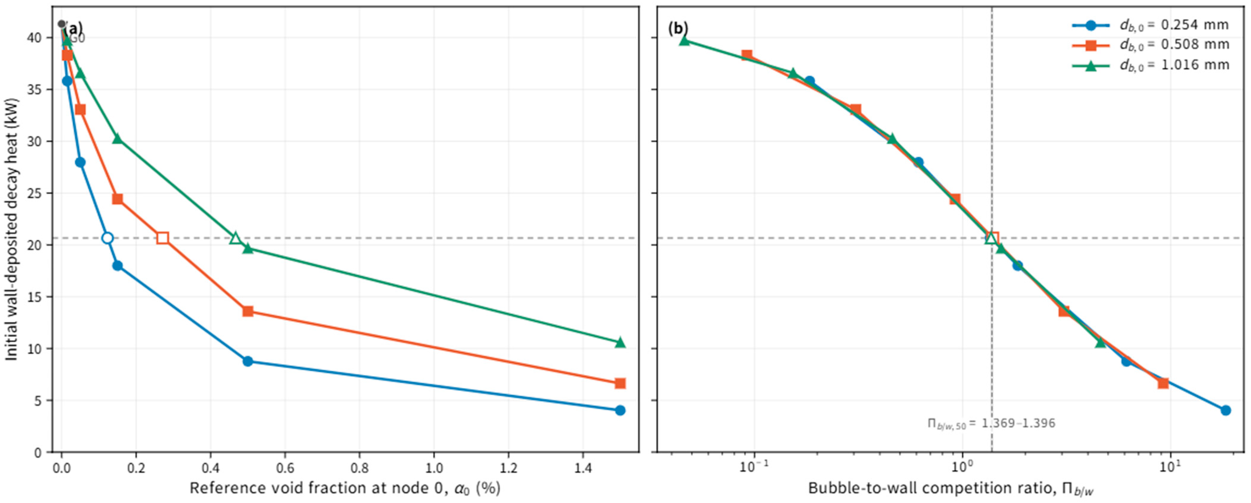
The first question examined was whether the operating void fraction affected the total wall-deposited decay heat at shutdown. As shown in Figure 4 and

Table 4. Initial wall-deposited decay heat within physical nodes 0–22 at shutdown.

Case	Reference Void Fraction at Node 0, (α0) (%)	Initial Wall-Deposited Decay Heat, ${\mathit{Q}}_{\mathbf{l}\mathbf{o}\mathbf{o}\mathbf{p}}\left(0\right)$ (kW)	Reduction Relative to G0 (%)
G0	0	41.329	0
G1	0.015	38.303	7.3
G2	0.050	33.063	20.0
G3	0.150	24.416	40.9
G4	0.500	13.595	67.1
G5	1.500	6.630	84.0

, for the baseline reference bubble diameter of 0.508 mm, the initial wall-deposited decay heat decreased monotonically from 41.33 kW in G0 to 6.63 kW in G5, corresponding to an overall reduction of 84.0%. A measurable response was already observed at low void fraction. Relative to G0, the initial wall-deposited decay heat decreased by 7.3% in G1, although its reference void fraction was only 0.015%; the reduction increased to 40.9% in G3 and 67.1% in G4. These results show that the operating void fraction substantially affected the magnitude of the wall-deposited decay heat source at shutdown and should therefore be considered when constructing post-drainage residual decay heat source terms.

Although the initial wall-deposited decay heat decreased monotonically over the investigated range, its response to the operating void fraction was distinctly nonlinear. When the decrease between adjacent cases was normalized by the corresponding increment in the reference void fraction, the reduction per 0.01 percentage point increment in ${\alpha }_0$ decreased from 2.02 kW over G0–G1 to 1.50, 0.86, 0.31, and 0.07 kW over G1–G2, G2–G3, G3–G4, and G4–G5, respectively. The largest marginal reduction therefore occurred in the low void fraction range, whereas progressively larger increments in void fraction were required to produce further decreases at higher void fractions. Nevertheless, the initial wall-deposited decay heat decreased by a further 6.97 kW from G4 to G5, indicating a diminishing marginal reduction rather than saturation within the investigated range. The origin of this nonlinear response cannot be identified from the total decay heat alone and is examined below through the spatial distribution and nuclide-specific inventory changes.

The bubble diameter sensitivity calculations showed that this qualitative response was preserved over the investigated bubble size range. For reference diameters of 0.254, 0.508, and 1.016 mm, the initial wall-deposited decay heat decreased monotonically with increasing operating void fraction, and the largest marginal reduction consistently occurred over G0–G1. At G5, the reductions relative to G0 were 90.26%, 83.96%, and 74.39%, respectively. Thus, the assumed bubble diameter affects the quantitative magnitude of the wall deposition reduction, but not the monotonic trend or the stronger response in the low void fraction range. The principal spatial ranking was also preserved across the three reference bubble diameters, with the heat exchanger remaining the largest component-level contributor and Node 14 the largest individual node.

The apparent bubble size dependence was substantially reduced when the same results were expressed in terms of the whole-loop bubble-to-wall nominal transfer-capacity ratio, ${\mathsf{\Pi }}_{b/w}$. The void fraction corresponding to a 50% reduction shifted from approximately 0.123% to 0.467% as the reference bubble diameter increased, whereas the corresponding half-response points collapsed to ${\mathsf{\Pi }}_{b/w}$ = 1.369–1.396. This indicates that the nonlinear transition is governed more directly by the relative bubble-to-wall transfer capacity than by the void fraction or bubble diameter considered separately.

3.2. Spatial Distribution and Post-Shutdown Evolution of the Wall-Deposition-Derived Decay Heat

3.2.1. Initial Spatial Distribution at Shutdown

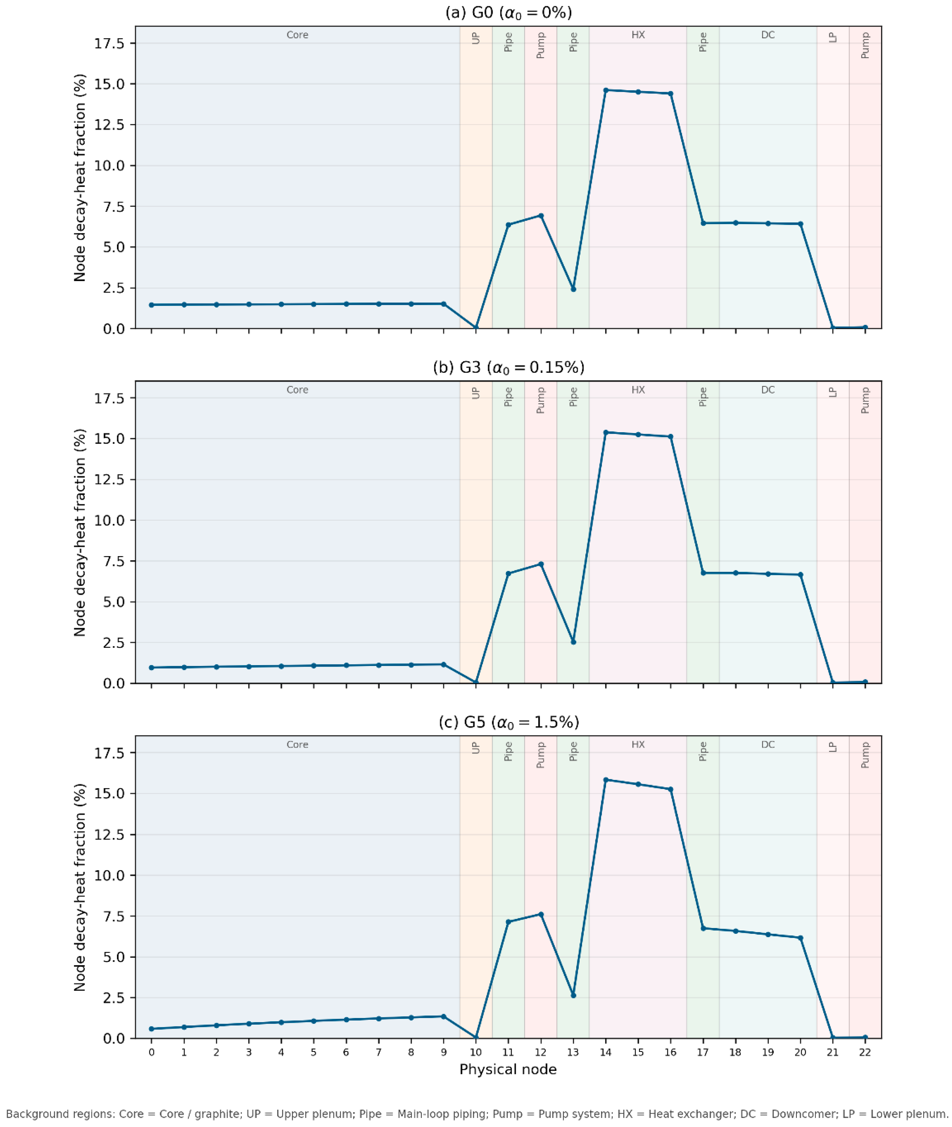
To separate changes in the relative spatial distribution from the large differences in total magnitude, the node-level decay heat in each case was normalized by the corresponding $Q_{\mathrm{l}\mathrm{o}\mathrm{o}\mathrm{p}}\left({\alpha }_m,0\right)$. Figure 5 shows the resulting node-level decay heat fractions for the representative G0, G3, and G5 cases. The normalized distribution was strongly nonuniform in all three cases. At the component level, the heat exchanger made the largest contribution, followed by the annular downcomer and primary-loop piping. The core/graphite region contributed a smaller fraction, whereas the upper and lower plena made very small contributions. The normalized distributions therefore show that the initial wall-deposited decay heat was concentrated mainly in external-loop components rather than being distributed uniformly among physical nodes 0–22.

At the physical-node scale, the normalized distributions in Figure 5 a–c retained the same principal spatial features across G0, G3, and G5. Node 14, the first node of the heat exchanger, had the largest fractional contribution in all three cases, increasing only modestly from approximately 14.6% in G0 to 15.8% in G5. Nodes 14–16 formed the principal high-contribution region within the heat exchanger, whereas node 17 and the annular downcomer nodes 18–20 formed a lower, broader secondary plateau in the downstream external loop. In the G0 case, the initial wall-deposited decay heats of the upper plenum (node 10), lower plenum (node 21), and pump bowl (node 22) were 17.582, 14.083, and 31.645 W. Their near-zero appearance in Figure 5 results from the linear plotting scale and their relatively low effective wall transfer capacities (see Table 2), rather than from assigning zero inventories or excluding these regions from the calculation. The persistence of these peaks, plateaus, and local minima indicates that increasing the operating void fraction did not change the location of the maximum fractional contribution or the primary spatial pattern.

Although the primary spatial pattern remained stable, closer comparison of the normalized profiles revealed a systematic secondary shift in the relative spatial distribution as the operating void fraction increased. From G0 to G5, the fractional contribution of the core/graphite region decreased from approximately 14.9% to 10.0%, whereas the heat exchanger fraction increased from 43.51% to 46.64%. Within core nodes 0–9, the nearly uniform G0 profile became increasingly weighted toward downstream nodes in G3 and G5, while the external-loop profiles changed more modestly. The operating void fraction therefore affected the total wall-deposited decay heat much more strongly than its normalized spatial distribution, but consistently shifted the relative contribution from the core toward the external loop. The bubble diameter sensitivity analysis further showed that the heat exchanger remained the largest component-level contributor, and Node 14 remained the maximum-contribution node for all investigated diameter–void fraction combinations. The principal component ranking was unchanged, and the maximum diameter-induced change in the component share was 1.321 percentage points.

3.2.2. Regional Post-Shutdown Evolution

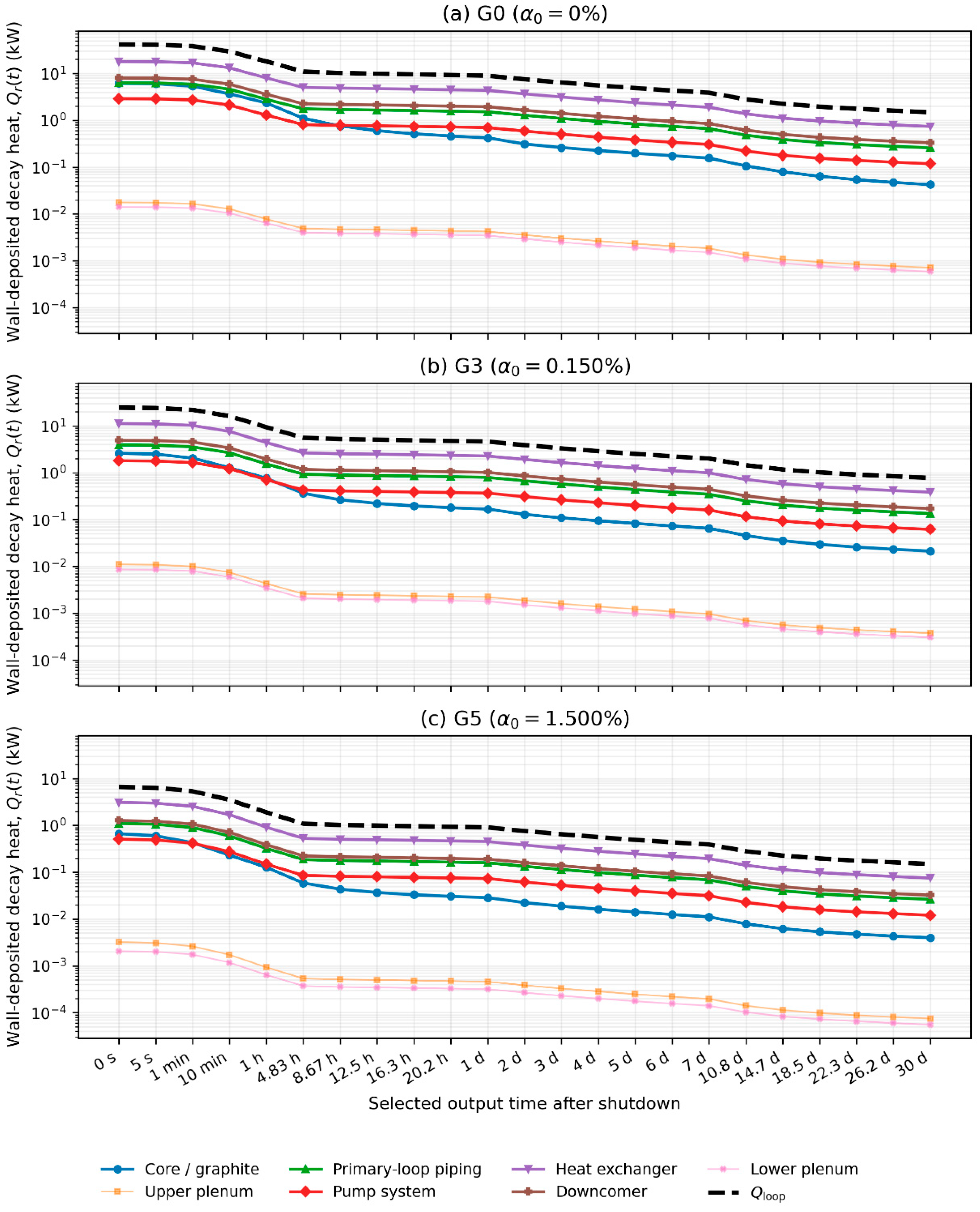
Following shutdown, the wall-deposited decay heat decreased continuously in all evaluated regions in G0, G3, and G5, as shown in Figure 6. However, the regional curves did not decrease proportionally, indicating that the post-shutdown spatial distribution was not a uniformly scaled version of the distribution at shutdown. The heat exchanger remained the largest contributor throughout the 30-day period, followed by the annular downcomer and primary-loop piping. In G3, the ratio $F_{\mathrm{H}\mathrm{X}}/F_{\mathrm{c}\mathrm{o}\mathrm{r}\mathrm{e}}$ increased from 1.347 at 1 h to 3.164 at 1 day and 4.231 at 30 days. At 30 days, the corresponding ratios for the annular downcomer and primary-loop piping were 4.297 and 4.218, respectively. These results show that the decay heat in the external-loop components decreased more slowly relative to their shutdown values than that in the core/graphite region, progressively increasing their relative contributions after shutdown.

A clear consequence of the differential regional decay behavior was the crossover between the pump system and the core/graphite region. At shutdown, the wall-deposited decay heat of the pump system was lower than that of the core/graphite region in all three cases, although the initial pump-to-core ratio increased from 0.471 in G0 to 0.694 in G3 and 0.767 in G5. Because the core/graphite decay heat decreased more rapidly, the pump-to-core ratio increased after shutdown and eventually exceeded unity. The first discrete outputs at which the pump system decay heat exceeded the core/graphite value occurred at 8.67 h in G0, 4.83 h in G3, and 10 min in G5, as summarized in

Table 5. Initial pump-to-core decay heat ratios and the first discrete output times at which the pump system decay heat exceeded that of the core/graphite region.

Case	Void Fraction at Node 0, (α0) (%)	Qpump(0)/Qcore(0)	First Discrete Output with (Qpump > Qcore)	(Qpump/Qcore) at That Output
G0	0	0.471	8.67 h	1.028
G3	0.150	0.694	4.83 h	1.174
G5	1.500	0.767	10 min	1.189

. These crossover times are quantitative results for the adopted baseline nodalization and component-level transport parameters; their exact values should therefore not be interpreted as geometry-independent predictions. At these outputs, the corresponding ratios $F_{\mathrm{p}\mathrm{u}\mathrm{m}\mathrm{p}}/F_{\mathrm{c}\mathrm{o}\mathrm{r}\mathrm{e}}$ were 2.182, 1.693, and 1.550 for G0, G3, and G5, respectively. Increasing the operating void fraction therefore reduced the initial difference between the core/graphite and pump system decay heats, causing the pump system contribution to exceed the core/graphite contribution earlier after shutdown. The nuclide composition differences underlying the faster reduction of the core/graphite decay heat and the greater relative persistence of the pump system contribution are examined in the subsequent analysis.

3.3. Nuclide Composition and Decay Chain Mechanisms of the Wall-Deposited Decay Heat

The preceding results showed that the operating void fraction affects both the magnitude and spatial distribution of the wall-deposited decay heat and its subsequent regional evolution. To identify the nuclide-level mechanisms underlying these responses, this section examines the temporal succession of dominant contributors, nuclide-specific inventory responses, regional compositional differences, and decay chain family evolution. Explicit precursor attribution is further used to distinguish inventories already present at shutdown from those generated by subsequent precursor feeding.

3.3.1. Temporal Succession and Concentration of Dominant Nuclide Contributions

The initial wall-deposited decay heat was distributed over a broad set of nuclides at shutdown. Even the highest-ranked nuclide accounted for only approximately 6–7% of the total in the representative cases. The breadth of the contribution distribution was quantified using $N_{50}$, $N_{90}$, and $N_{99}$, as defined in Section 2.3.3. As summarized in

Table 6. Number of nuclides required to reach selected cumulative contributions to the initial wall-deposited decay heat.

Case	N50,Q	N90,Q	N99,Q
G0	10	35	78
G3	10	39	83
G5	13	48	94

, in G0, 10, 35, and 78 nuclides were required to reach cumulative contributions of 50%, 90%, and 99%, respectively. The contribution distribution became less concentrated as the operating void fraction increased. In G5, $N_{50}$, $N_{90}$, and $N_{99}$ increased to 13, 48, and 94, respectively. The complete ranked nuclide lists corresponding to $N_{50,Q}$, $N_{90,Q}$, and $N_{99,Q}$ at shutdown, together with their individual and cumulative decay heat contributions, are provided in Supplementary Table S1. The broadening was more evident in $N_{90}$ and $N_{99}$ than in $N_{50}$, indicating that the operating void fraction primarily increased the number of secondary contributors required to represent the initial decay heat source.

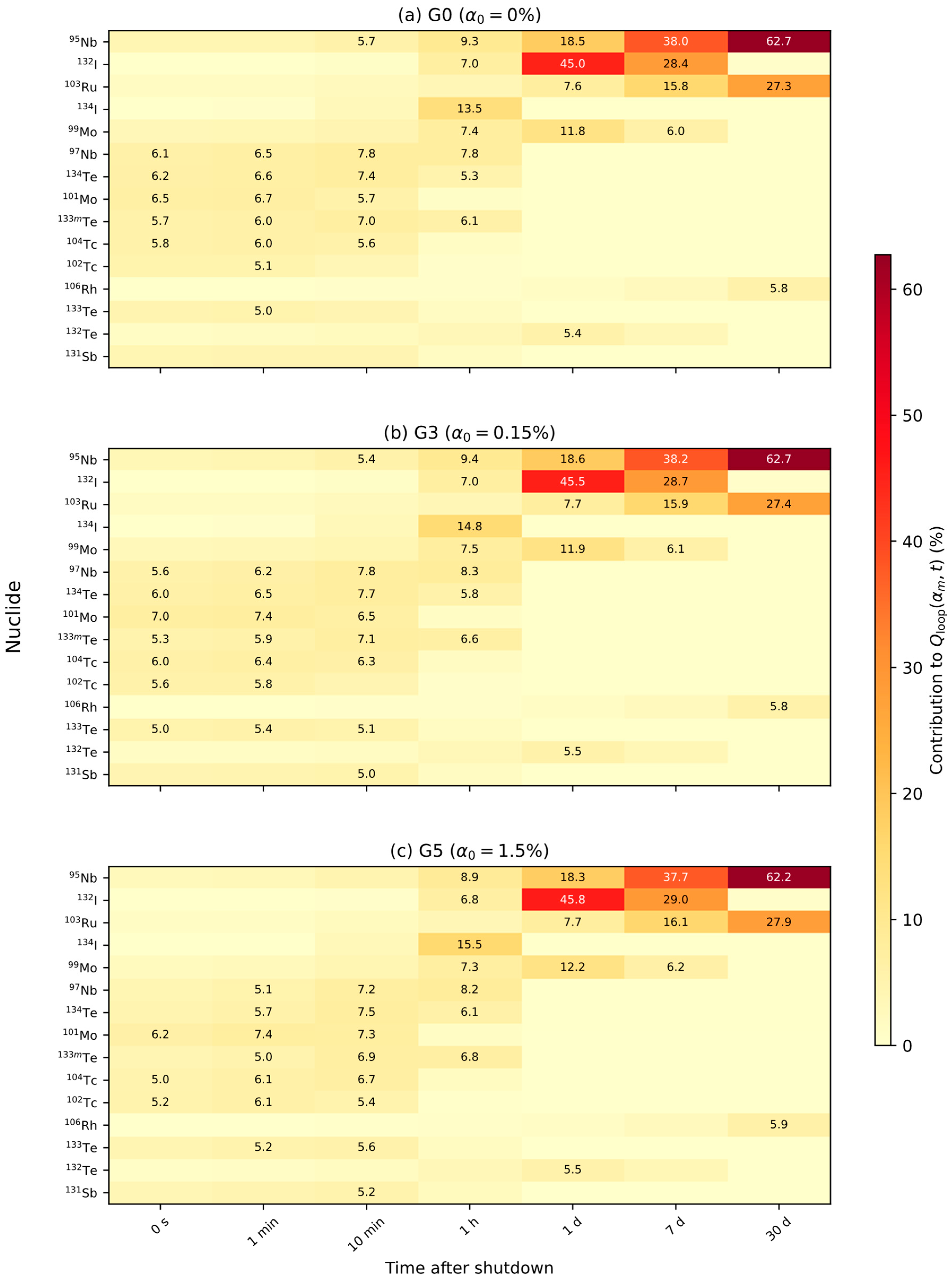
Figure 7 shows the stagewise succession of the dominant nuclide contributions in G0, G3, and G5. The 15 displayed nuclides were selected according to their maximum decay heat fractions over the 21 representative case–time combinations, with the complete rankings provided in Supplementary Table S2. At shutdown and 1 min thereafter, the decay heat remained broadly distributed among Mo, Nb, Te, and Tc nuclides. In all three cases, ¹⁰¹Mo ranked first at these early times but contributed only 6.22–7.40% of $Q_{\mathrm{l}\mathrm{o}\mathrm{o}\mathrm{p}}$. At 10 min, ⁹⁷Nb ranked first in G0 and G3, contributing approximately 7.8%, whereas the ranking in G5 remained closely contested, with ¹³⁴Te, ¹⁰¹Mo, and ⁹⁷Nb contributing 7.5%, 7.3%, and 7.2%, respectively. By 1 h, ¹³⁴I had become the leading contributor in all three cases, accounting for 13.5–15.5%, while ⁹⁵Nb, ⁹⁷Nb, and ⁹⁹Mo remained important secondary contributors. At 1 day, the contribution distribution became substantially more concentrated, with ¹³²I accounting for 45.0–45.8%, followed by ⁹⁵Nb at 18.3–18.6% and ⁹⁹Mo at 11.8–12.2%. By 7 days, ⁹⁵Nb had replaced ¹³²I as the leading contributor, accounting for 37.7–38.2%, while ¹³²I and ¹⁰³Ru contributed 28.4–29.0% and 15.8–16.1%, respectively. By 30 days, the decay heat was dominated by ⁹⁵Nb and ¹⁰³Ru, which together accounted for approximately 90% of $Q_{\mathrm{l}\mathrm{o}\mathrm{o}\mathrm{p}}$, while ¹⁰⁶Rh provided a further 5.8–5.9%. The operating void fraction primarily affected the detailed ranking of closely competing nuclides during the first several minutes after shutdown. Thereafter, all three cases followed the same overall succession from ¹³⁴I to ¹³²I and finally to ⁹⁵Nb and ¹⁰³Ru.

The stagewise succession of the leading contributors was accompanied by a marked concentration of the nuclide contribution distribution. The cumulative contribution metrics were used only to quantify the evolving breadth of the dominant-nuclide set. The dominant-nuclide distribution therefore became progressively more concentrated with time: $N_{90}$ decreased from 35–48 at shutdown to 2 at 30 days, when ⁹⁵Nb and ¹⁰³Ru together contributed approximately 90% of the decay heat. Thus, although increasing the void fraction broadened the initial contribution distribution, all three cases converged toward a similarly concentrated long-term pattern, demonstrating that a single shutdown ranking is insufficient to represent the full post-shutdown period.

3.3.2. Nuclide-Specific Shutdown Inventory Responses and Their Decay Chain Evolution

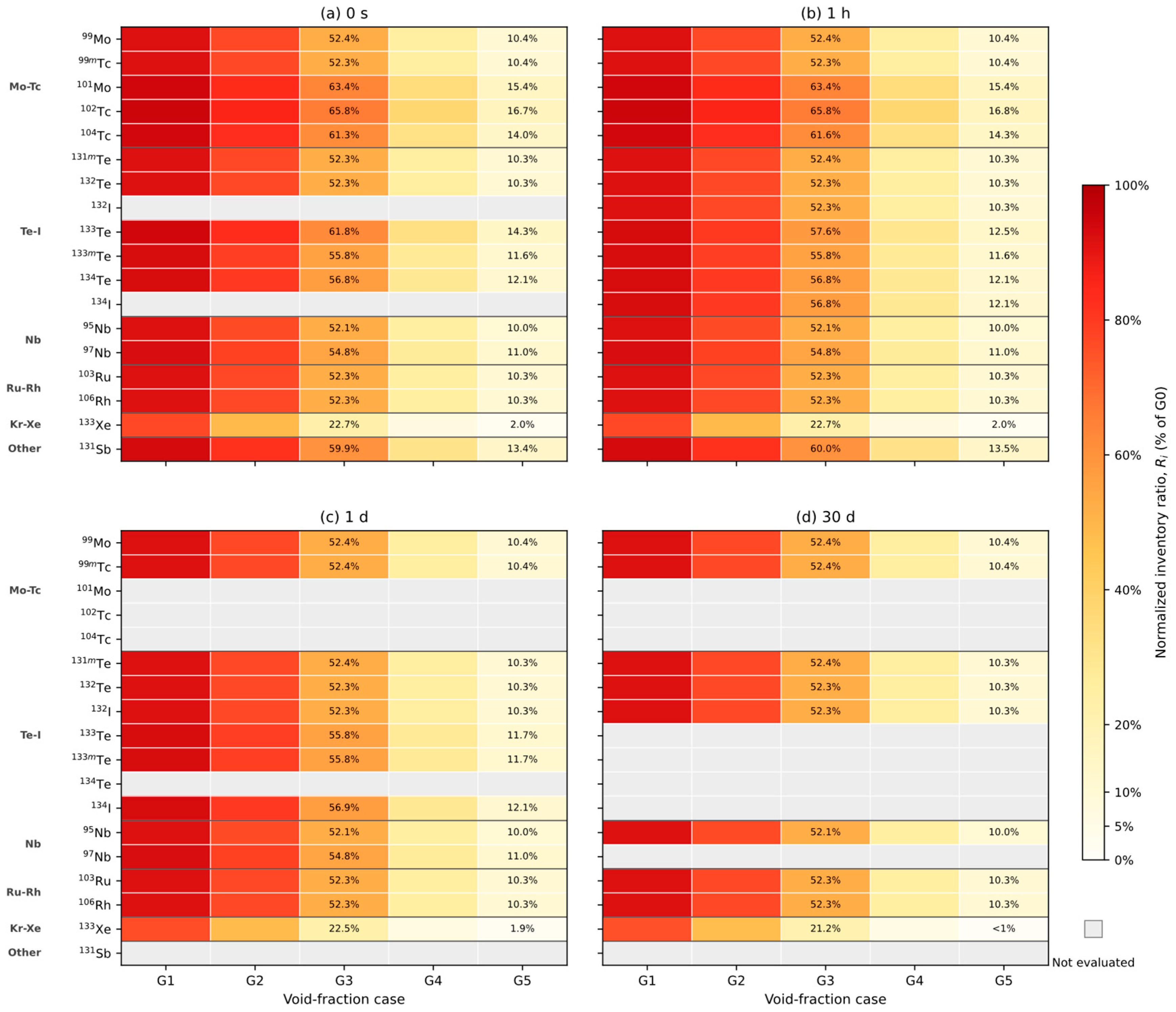
All void fraction cases were evolved using the same post-shutdown decay equation. The differences examined here therefore reflect the nuclide-specific wall-associated inventories established at shutdown and their subsequent decay chain evolution, rather than continued void-fraction-dependent transport. Figure 8 compares the normalized inventory ratios of selected nuclides relative to G0 at 0 s, 1 h, 1 day, and 30 days. For a given nuclide, this inventory ratio is also equal to its decay heat ratio because its decay constant and recoverable energy per decay is identical across cases. Complete nuclide selection records and normalized inventory ratios are provided in Supplementary Table S3. For a given nuclide, this ratio is also equal to its decay heat ratio because its decay constant and recoverable energy per decay is identical across cases. Increasing the operating void fraction reduced the inventories of nearly all evaluated nuclides, but the reduction was nuclide-dependent. Most displayed nuclides in G3 retained approximately 52–66% of the corresponding G0 inventories, whereas most values in G5 were approximately 10–17%. At shutdown, for example, the G5/G0 ratios were 9.98% for ⁹⁵Nb, 10.28% for ¹⁰³Ru, and 16.74% for ¹⁰²Tc, compared with only approximately 2% for ¹³³Xe. Thus, the higher-void cases cannot be represented by a uniform scaling of the G0 nuclide inventory pattern.

The normalized inventory ratio of a given nuclide generally changed only slightly after shutdown when its evolution was dominated by the inventory already present at shutdown. In G5, for example, the ratio for 95Nb remained approximately 9.98% at all four evaluated times, while those of several Mo–Tc, Te–I, and Ru–Rh nuclides remained close to 10%. This behavior results from the common post-shutdown decay kinetics applied to all cases, which approximately preserves the intercase ratio in the absence of substantial precursor feeding. For daughter nuclides, however, the ratio can evolve as upstream precursor contributions become important. Similar responses within the ⁹⁹Mo–^99mTc and ¹³²Te–¹³²I chain illustrate the transfer of the precursor shutdown response to daughter inventories. This behavior was not universal; for ¹³³Xe, the G5/G0 normalized inventory ratio decreased from approximately 2.03% at shutdown to below 1% at 30 days. Thus, the nuclide-specific response established at shutdown can either persist through subsequent decay or be modified through precursor feeding.

Figure 7 and Figure 8 further distinguish changes in absolute nuclide inventories from changes in their fractional contributions to the total decay heat. A nuclide can contribute a larger fraction in a higher-void case even when its absolute inventory is lower, provided that its inventory decreases less than the total wall-deposited source. At 1 h, for example, the ¹³⁴I inventory in G5 was only 12.09% of that in G0, whereas its fractional contribution increased from 13.5% in G0 to 15.5% in G5. The same pattern was observed for ¹³²I at 1 day and ¹⁰³Ru at 30 days. Thus, the increased fractional contributions of these nuclides reflect differences in their relative inventory reductions rather than increases in their absolute decay heat.

3.3.3. Regional Nuclide Composition and Differential Decay Behavior

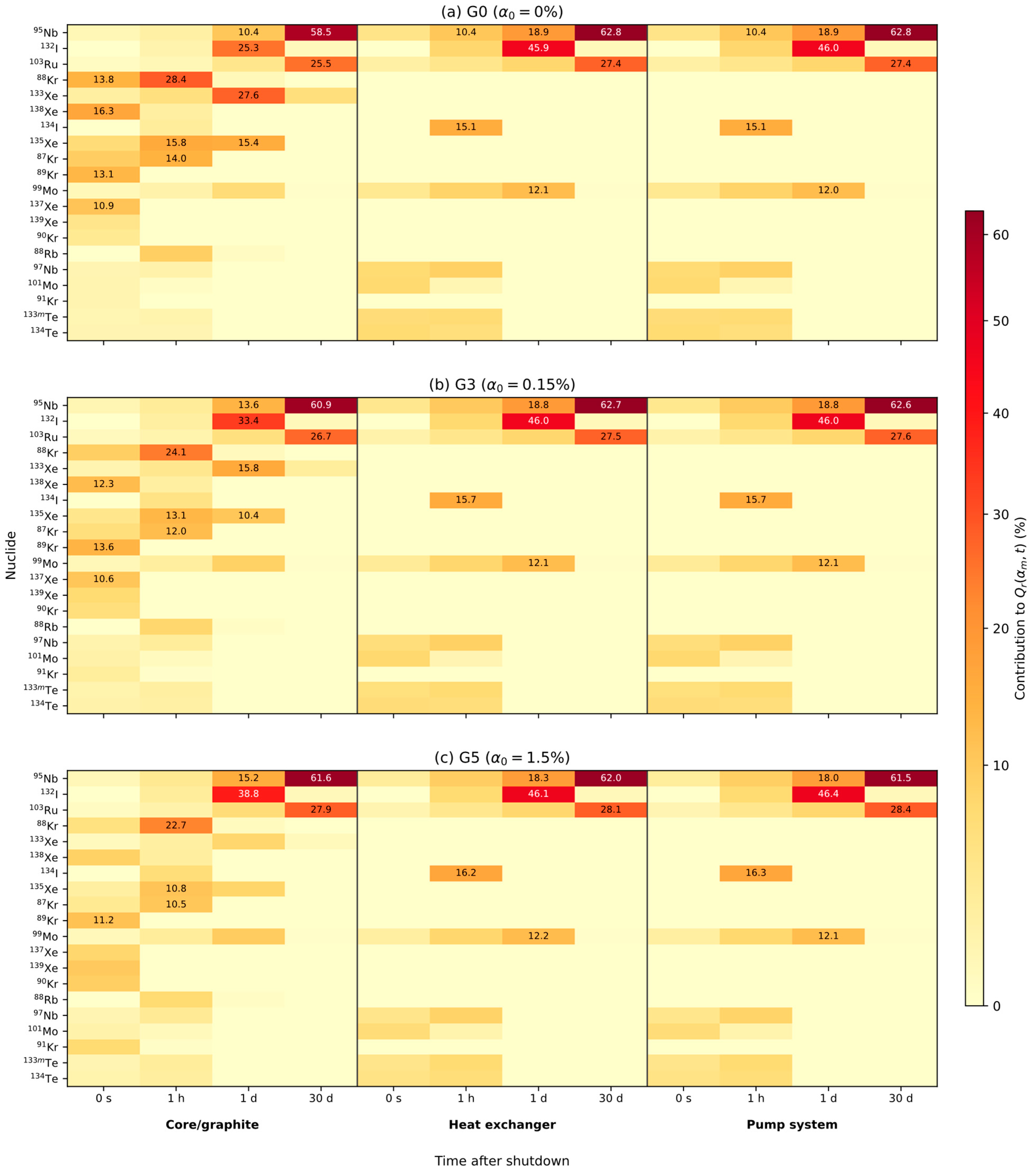
Figure 9 compares the regional nuclide compositions of wall-deposited decay heat in the core/graphite region, heat exchanger, and pump system for G0, G3, and G5. Complete regional rankings and display selection records are provided in Supplementary Table S4. At shutdown, the nuclide contribution distribution in the core differed clearly from those in the heat exchanger and pump system. The initial core decay heat contained large contributions from short-lived Kr and Xe nuclides. In G0, for example, ¹³⁸Xe, ⁸⁸Kr, ⁸⁹Kr, and ¹³⁷Xe accounted for 16.3%, 13.8%, 13.1%, and 10.9%, respectively. In contrast, the initial distributions in the heat exchanger and pump system showed no comparable dominance by Kr and Xe nuclides and were more broadly distributed among Mo, Nb, Te, and other contributors. Increasing the operating void fraction reduced the relative importance of several short-lived Kr and Xe nuclides in the core but did not remove this regional contrast. The higher short-lived nuclide contribution in the core helps explain its more rapid early decay heat reduction.

The regional compositional differences persisted during the early and intermediate post-shutdown periods. At 1 h, the combined contribution of ⁸⁸Kr, ¹³⁵Xe, and ⁸⁷Kr to the core/graphite decay heat remained 44.0–58.2% across the three cases, whereas ¹³⁴I had become the largest contributor in both the heat exchanger and pump system at approximately 15–16%. At 1 day, ¹³²I dominated the two external-loop regions, contributing 45.9–46.4%, while its contribution in the core increased from 25.3% in G0 to 38.8% in G5, and short-lived Xe remained important. As the Kr and Xe contributions declined, the core composition therefore evolved more rapidly than those of the heat exchanger and pump system. By 30 days, however, the regional compositions had largely converged: ⁹⁵Nb and ¹⁰³Ru together accounted for 84.0–89.5% of the core/graphite decay heat and approximately 90% in the heat exchanger and pump system. Regional differences in decay heat evolution were therefore governed mainly by the timing and relative weights of nuclide succession during the early and intermediate periods.

The decay heat of a region at any post-shutdown time is jointly determined by its initial value at shutdown and its normalized remaining fraction. Accordingly, the decay heat ratio of region $r$ relative to the core/graphite region can be decomposed as:

$${\displaystyle \frac{Q_r\left(t\right)}{Q_{\mathrm{c}\mathrm{o}\mathrm{r}\mathrm{e}}\left(t\right)}}={\displaystyle \frac{Q_r\left(0\right)}{Q_{\mathrm{c}\mathrm{o}\mathrm{r}\mathrm{e}}\left(0\right)}}{\displaystyle \frac{F_r\left(t\right)}{F_{\mathrm{c}\mathrm{o}\mathrm{r}\mathrm{e}}\left(t\right)}}.$$

(23)

where $F_j\left(t\right)=Q_j\left(t\right)/Q_j\left(0\right)$ is the normalized remaining fraction of region $j$. In G3, the heat exchanger-to-core decay heat ratio was 4.301 at shutdown; its slower subsequent reduction increased the normalized remaining fraction ratio to 4.231 at 30 days, giving a decay heat ratio of approximately 18.2. The pump system showed the complementary behavior: although its initial decay heat was only 0.694 times that of the core, its slower reduction caused the pump contribution to exceed the core contribution at the 4.83 h output. Thus, the sustained dominance of the heat exchanger and the later pump-to-core crossover both result from the combined effects of the initial regional inventory distribution and the region-dependent nuclide composition.

3.3.4. Decay Chain Family Evolution and Explicit Precursor Attribution

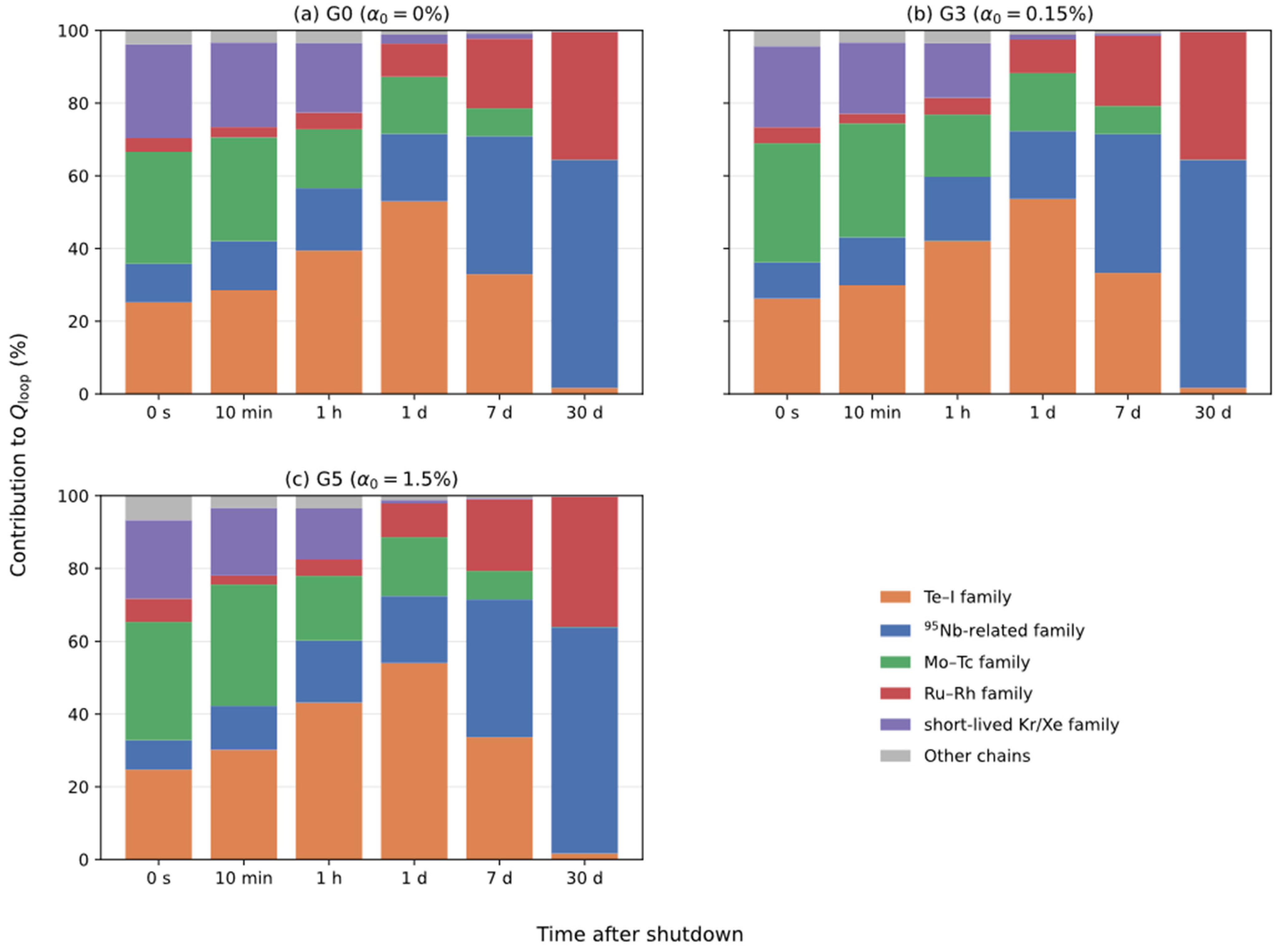
To interpret the nuclide succession at the family level, Figure 10 compares the fractional contributions of the six mutually exclusive mass-number-based families constructed using the grouping procedure described in Section 2.3.4. At shutdown, the decay heat was broadly distributed, with the Mo–Tc, Te–I, and short-lived Kr/Xe families contributing approximately 30–33%, 25–26%, and 22–27%, respectively. The complete family assignments are provided in Supplementary Table S5. The Te–I contribution increased to approximately 40–43% at 1 h and reached 53–54% at 1 day. By 7 days, the 95Nb-related family had become the largest contributor at approximately 38–39%. At 30 days, the 95Nb-related and Ru–Rh families contributed approximately 63–64% and 34–36%, respectively, and together accounted for nearly all of the remaining wall-deposited decay heat. Thus, all three representative void fraction cases followed the same overall family-level succession: an initially distributed pattern, followed by Te–I dominance and finally by 95Nb-related and Ru–Rh dominance.

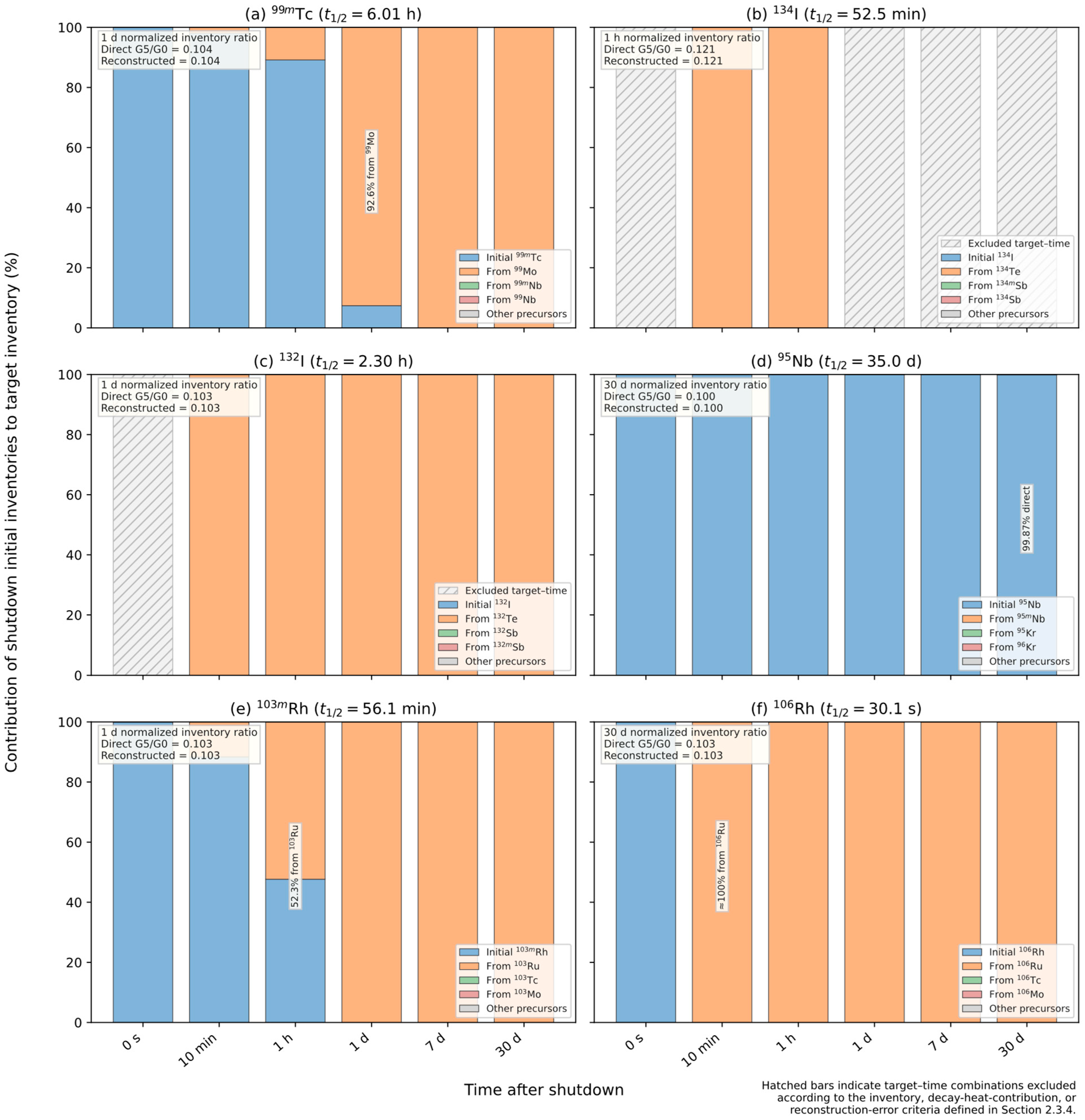
Family-level grouping identifies the dominant decay chain groups but does not determine whether a target nuclide is sustained by its own shutdown inventory or by upstream precursor feeding. Explicit precursor attribution was therefore applied to the 19 target nuclides selected in Section 2.3.4. Figure 11 shows six representative targets for G3 and separates the surviving contribution of each target inventory present at shutdown from contributions generated by upstream shutdown inventories. The complete attribution results for all 19 targets are provided in Supplementary Table S7.

The selected targets exhibited three characteristic attribution patterns. First, ¹³⁴I and ¹³²I were precursor-dominated, with their inventories generated almost entirely from the shutdown inventories of ¹³⁴Te and ¹³²Te, respectively. Second, ⁹⁵Nb remained dominated by its own shutdown inventory, which still accounted for 99.87% of its inventory at 30 days. Third, ^99mTc and the Ru–Rh daughters showed time-dependent transitions from target inventory dominance to precursor feeding dominance. For ^99mTc, its own shutdown inventory accounted for 89.16% of the target inventory at 1 h, whereas feeding from ⁹⁹Mo accounted for 92.60% at 1 day. The Ru–Rh pathways showed the same transition on shorter time scales: ¹⁰³Ru became the dominant source of ^103mRh, and ¹⁰⁶Rh was generated almost entirely from ¹⁰⁶Ru from 10 min onward. These results show that the persistence of a target nuclide cannot be inferred from its own half-life alone; the inventories and decay characteristics of upstream precursors may also control its post-shutdown contribution.

Figure 11 also compares the directly calculated G5/G0 normalized inventory ratios with those reconstructed from the G0 attribution fractions and the G5/G0 ratios of the contributing shutdown inventories. The reconstructed ratios agreed with the direct calculations on the reported precision for all six displayed targets, confirming numerical closure of the attribution and response reconstruction. The Te–I daughter responses were controlled primarily by their Te precursor inventories, whereas the ⁹⁵Nb response was controlled almost entirely by its own shutdown inventory. For ^99mTc and the Ru–Rh daughters, the controlling response shifted with time from the target inventory to the corresponding precursor inventory. The post-shutdown response of a daughter nuclide is therefore determined by the attribution-weighted responses of the shutdown inventories that contribute to it.

Taken together, the family and precursor analyses show that post-shutdown decay heat evolution is governed by both decay chain succession and the origin of the inventories entering those chains. The operating void fraction changes the shutdown inventories and therefore the magnitudes and relative contributions propagated through the decay network, but it does not change the intrinsic decay kinetics. A representative decay heat source must therefore account for both the time-dependent set of important nuclides and precursor feeding rather than rely only on the shutdown ranking or the half-lives of individual target nuclides.

3.4. Implications for Shutdown Decay Heat Representation and Analysis

The preceding results show that a single spatially lumped decay heat curve is insufficient to represent the wall-deposited source. The operating void fraction affects the shutdown magnitude, spatial distribution, and nuclide composition, while the regional decay heat curves and nuclide-specific inventory responses do not scale proportionally with the G0 case. Source-term representations should therefore retain the operating condition dependence, component- or region-level spatial distribution, post-shutdown time dependence, and relevant precursor relationships. The present results provide a basis for constructing such void-fraction-dependent, component-resolved source terms rather than applying a single correction factor to a fixed global source.

The component-level results further show that the relative importance of individual regions changes with the post-shutdown time. The heat exchanger remained the largest contributor and decayed more slowly than the core, so a core-based decay heat curve would underrepresent the persistent heat exchanger source. The core decreased more rapidly because of its different initial nuclide composition, whereas the pump contribution eventually exceeded that of the core, with the crossover time depending on the operating void fraction. These behaviors support a component-resolved and time-dependent representation rather than a source distribution fixed at shutdown.

The calculated sources can serve as inputs to subsequent thermal–hydraulic analyses of component temperatures, heat removal requirements, and other post-shutdown responses under specified system and boundary conditions. However, the present results do not directly determine component temperatures, cooling requirements, salt freezing margins, or shutdown safety because these quantities also depend on heat capacity, heat transfer, salt circulation, cooling system operation, and thermal boundary conditions. In particular, the more rapid reduction in core decay heat does not by itself imply a greater salt freezing risk. Likewise, neither an optimal drainage time nor an optimal operating void fraction can be inferred from the present source-term results alone because a finite-duration drainage transient simultaneously changes the salt inventory, source location, flow paths, and cooling conditions. Further work should therefore couple the present decay heat source model with transient salt drainage and thermal–hydraulic analyses.

4. Conclusions and Future Work

This study investigated how the operating void fraction affects the wall-deposited fission product inventory and the resulting shutdown decay heat in the main loop of a molten salt reactor. Six operating cases with reference void fractions ranging from 0 to 1.5% were considered. The wall-associated inventories in physical nodes 0–22 at shutdown were used as the initial source under an idealized post-drainage condition, and their subsequent evolution was calculated using radioactive decay and daughter nuclide ingrowth only. The reported decay heat therefore represents this residual component-associated source rather than the total post-shutdown decay heat of the reactor.

Three principal conclusions were obtained. First, the operating void fraction strongly affected the magnitude of the residual source. For the baseline bubble diameter of 0.508 mm, the initial wall-deposited decay heat decreased monotonically from 41.33 kW in G0 to 6.63 kW in G5, corresponding to an 84.0% reduction. Bubble diameter sensitivity calculations preserved the monotonic trend and the stronger response in the low void fraction range, although the quantitative reduction depended on the bubble diameter. Second, the source remained strongly nonuniform. The heat exchanger was consistently the largest component-level contributor, while increasing the void fraction reduced the core fraction and increased the relative external-loop contribution. The core decayed more rapidly because of its larger initial contribution from short-lived Kr and Xe nuclides, and the pump system contribution subsequently exceeded that of the core at a void-fraction-dependent time. Third, the nuclide composition evolved from a broad initial distribution to a concentrated long-term source: $N_{90,Q}$ decreased from 35 to 48 at shutdown to 2 at 30 days, when ⁹⁵Nb and ¹⁰³Ru together contributed approximately 90% of the decay heat. The operating void fraction affected individual shutdown inventories nonuniformly, while precursor feeding transferred these inventory responses through important decay chains.

These findings link operating period multiphase transport to the magnitude, spatial distribution, and nuclide composition of the residual decay heat source retained on primary-loop components. Shutdown source terms for this contribution should therefore retain operating condition dependence, component-level spatial resolution, time dependence, and relevant precursor relationships rather than rely on a single main-loop curve or uniform scaling factor. The present results provide source-term inputs for subsequent thermal–hydraulic and system analyses, but do not by themselves determine component temperatures, cooling requirements, salt-freezing margins, or an optimal drainage or operating strategy. These quantities require coupled treatment of the decay heat source, salt drainage, heat transfer, circulation, and cooling system boundary conditions.