Heat Transfer Performance of a Multi-Branch Well System for In-Situ Conversion of Steeply Dipping Oil Shale Reservoirs

Abstract

Efficient heat transfer is essential for the in-situ conversion of steeply dipping oil shale reservoirs. In this study, a superheated steam-driven integrated multi-branch well system was proposed, and a coupled thermo-hydro-chemical-mass transport model considering reservoir anisotropy was established in COMSOL Multiphysics-5.6 to investigate heat transfer characteristics and evaluate the effects of key engineering parameters. The numerical model was validated through comparison with an analytical solution and previously published numerical results. The results show that superheated steam preferentially migrates through hydraulic fractures and bedding-parallel high-permeability pathways, resulting in anisotropic heat transfer. Continuous steam injection gradually forms a connected high-temperature region, and most of the reservoir exceeds 500 °C after approximately 600 days. Compared with the conventional well arrangement, the proposed well system achieves more uniform reservoir heating and enlarges the effective pyrolysis region. Parametric analysis indicates that the highest thermal performance among the investigated cases is obtained with a heating well length of 22.5 m, while increasing the inter-well angle, fracture number, and fracture width enhances heat transfer and kerogen conversion. Among the investigated cases, the configuration with three hydraulic fractures achieves the best performance, with the high-temperature region (>500 °C) exceeding 80% of the reservoir after 400 days and a cumulative hydrocarbon production of approximately 4.7 × 10⁷ mol. Sensitivity analysis further demonstrates that fracture-related parameters exert a greater influence on reservoir thermal performance than heating well length and inter-well angle. These findings provide theoretical guidance for the design and performance evaluation of integrated multi-branch well systems for the efficient in-situ conversion of steeply dipping oil shale reservoirs.

1. Introduction

Oil shale is a low-permeability sedimentary rock containing immature kerogen, which is immobile under natural conditions. Through pyrolysis and other thermochemical conversion processes, its organic matter can be fractured to produce shale oil and natural gas, which can be further refined into liquid fuels or chemical feedstocks [1,2]. According to the latest national resource assessment (2023), China possesses approximately 7.199 trillion tons of identified oil shale resources, ranking among the largest oil shale resource holders worldwide [3]. The recoverable shale oil reserves are about 47.6 billion tons, ranking second in the world. In comparison, conventional recoverable petroleum reserves are only about 26.8 billion tons, indicating that oil shale represents a resource potential far exceeding that of conventional oil [4].

Oil shale extraction technologies can generally be classified into two main approaches. The first is surface retorting, in which oil shale is mined and then heated at the surface for pyrolysis. Although this method is technologically mature, it suffers from a large land footprint, severe ecological disturbance, and difficulties in controlling solid waste and gaseous emissions, making it unsuitable for deep resources. The second approach is in-situ conversion, which heats oil shale directly underground through subsurface systems. This method is more suitable for deep reservoirs and offers lower environmental impact, reduced solid waste and chemical residues, as well as higher resource utilization efficiency and better environmental compatibility [5,6]. Zhao et al. proposed a superheated steam-based in-situ convective heating method (MTI technology), in which injection and production wells are drilled from the surface, and hydraulic fracturing is used to create long fractures along parallel bedding planes, connecting injection and production wells [7]. High-temperature steam is injected into the oil shale formation to heat the organic matter, promoting its thermal decomposition into oil and gas, which are then produced through production wells. Meanwhile, steam-boiling-induced erosion can enhance formation permeability and accelerate heating. Song et al. investigated the use of high-temperature fluid injection in horizontal wells for oil shale heating and analyzed the influence of well configurations on heating efficiency. However, the extremely low vertical permeability of oil shale was not fully considered, resulting in limited heat transfer efficiency and an effective heating distance of only about 20 m [8]. Song et al. analyzed the numerical simulation results and reported that the temperature within 80 cm of the heating source exceeded 350 °C, which was sufficient to initiate the pyrolysis of asphaltenes into hydrocarbons. However, the temperature decreased rapidly with increasing distance from the heating well, and regions farther away failed to reach the fracturing temperature required for efficient pyrolysis, thereby limiting the overall conversion efficiency [9]. Li et al. demonstrated that current in-situ oil shale extraction technologies still suffer from several limitations, including low energy utilization efficiency and high energy consumption, indicating that considerable challenges remain before large-scale commercial application can be achieved [10]. Lei et al. compared different well configurations through numerical simulations and found that a hexagonal well pattern achieved higher production efficiency than triangular and quadrilateral layouts under the same energy input, owing to its larger effective heating coverage. Their results also identified an optimal well spacing of 16 ft. Nevertheless, the effective heat transfer range remained relatively limited, highlighting the need for parametric analysis of heat transfer performance in in-situ heating systems [11]. Existing studies indicate that current in-situ heating methods still face several critical limitations under complex reservoir conditions. On the one hand, low vertical permeability significantly restricts the propagation of thermal fluids within the reservoir, thereby limiting the heating extent. On the other hand, single-well configurations or conventional horizontal well patterns show poor adaptability in heterogeneous and inclined formations, making it difficult to achieve coordinated multiscale heating and balanced injection–production control. Therefore, improving heat transfer efficiency and enlarging the effective heated volume under complex geological conditions remains a key challenge for enhancing the efficiency of in-situ conversion processes.

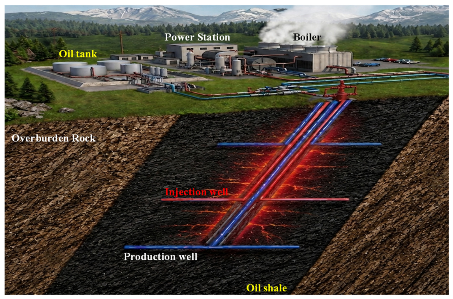
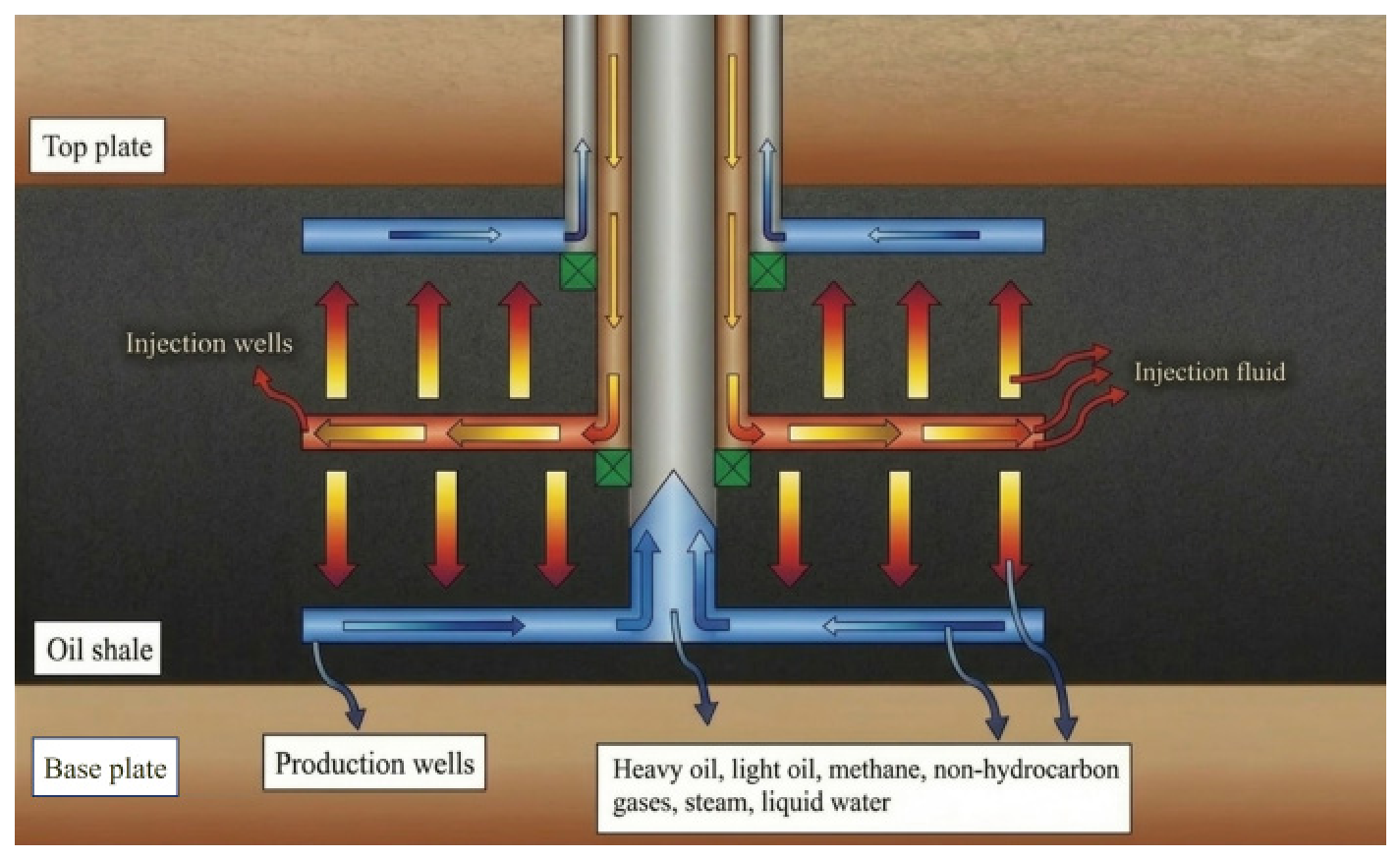
Zhang et al. developed a three-dimensional thermo-hydro-chemical coupled model to investigate heat transfer and kerogen decomposition. Their study identified two key performance indicators and determined both a minimum power threshold, below which kerogen decomposition could not be initiated, and a maximum power threshold, beyond which additional energy input produced only marginal improvements in conversion efficiency [12]. Furthermore, Zhu et al. established a multiphysics model incorporating electromagnetic heating, heat transfer, chemical reactions, and mass transport to evaluate the effects of microwave power and the thermal conductivity of oil shale on reservoir temperature distribution. Their results demonstrated that microwave irradiation significantly enhanced the porosity and permeability of oil shale, while the combination of microwave heating and hydraulic fracturing further improved the permeability of the reservoir by creating more effective seepage pathways [13]. Most numerical studies on in-situ conversion of oil shale assume horizontally layered formations. However, in engineering practice, oil shale reservoirs are rarely ideally horizontal. Taking the Jimusar area in Xinjiang, China as an example, the oil shale in this region is a typical lacustrine sediment deposited in a continental basin. Due to tectonic movements, the formation dip varies significantly, with well-developed bedding planes and spatially heterogeneous cementation strength, which poses substantial challenges to well placement strategies based on horizontal formation assumptions [14,15]. Wang et al. investigated the in-situ recovery of inclined oil shale and compared the temperature and pressure field evolution between wells drilled parallel to bedding and those perpendicular to bedding [16]. The results show that wells aligned parallel to bedding achieve higher heating efficiency in the early production stage, whereas wells oriented perpendicular to bedding are more favorable for improving energy recovery efficiency in the later stage. In addition, parallel-bedding drilling can effectively prevent wellbore shear failure and reduce drilling costs, with optimal performance achieved when four hydraulic fracture planes are used. However, this approach requires at least three main wells, and the fracture planes must be oriented perpendicular to bedding. Owing to the difficulty of fracture propagation in the direction perpendicular to bedding, fracture length is limited, resulting in lower production rates, high initial investment, and a long payback period. In this study, the integrated multi-branch well system (Figure 1) refers to a single-main-well configuration consisting of multiple branch wells for steam injection and hydrocarbon production. Compared with conventional multilateral wells, the proposed configuration integrates injection and production functions within one coordinated well network to improve reservoir heating efficiency. This well configuration can effectively avoid wellbore shear failure induced by formation slippage, significantly reduce initial drilling costs, and facilitate the creation of large-area hydraulic fracture networks, thereby offering substantially improved economic performance compared with conventional bedding-parallel well configurations. For clarity in analyzing the structural characteristics of this novel well pattern, a simplified planar representation is adopted, as shown in Figure 2. As illustrated, the system is centered on a single main well, from which multiple branch wells extend at different depths along the reservoir, forming a multi-branch well system. An injection well is arranged in the middle section to continuously inject high-temperature superheated steam into the reservoir. After entering the formation, the steam preferentially propagates along fractures and high-permeability channels, enabling rapid, large-scale, and relatively uniform reservoir heating. Meanwhile, production wells are arranged above and below the well network to achieve coordinated injection–production control and efficient matching between injection and production. During production, part of the heat carried by high-temperature steam is transferred to the produced fluids within the inner and outer tubing, thereby reducing the rate of high-temperature oxidation and corrosion in the wellbore and near-wellbore regions [17,18]. In addition, the downward-flowing superheated steam continuously reheats the produced fluids, effectively inhibiting the precipitation of heavy components and high-freezing-point substances (such as wax) on low-temperature tubing walls, thereby reducing the risk of wax deposition and flow blockage [19,20]. Overall, this technology enhances heating efficiency and production stability through optimized injection–production coupling and wellbore thermal management, while effectively mitigating key engineering issues such as pipeline corrosion and wax deposition in conventional in-situ conversion processes.

Although previous studies have investigated horizontal wells, multilateral wells, and hydraulic fracturing-assisted heating strategies for oil shale in-situ conversion, most existing studies focus on horizontally layered reservoirs and mainly optimize individual well parameters. The influence of steeply dipping geological structures on steam migration, anisotropic heat transfer, and the coupled evolution of pyrolysis efficiency remains insufficiently understood. In particular, conventional well arrangements require multiple parallel wells and are difficult to adapt to steeply inclined reservoirs due to increased drilling complexity and limited fracture propagation. In this study, a superheated steam-based in-situ convective heating method is proposed for steeply inclined oil shale. Taking the Jimusar oil shale deposit in Xinjiang as the research object, a coupled thermo–hydro–chemical–transport mathematical model is established with consideration of formation dip effects. The dynamic evolution of velocity, pressure, temperature fields, and organic matter conversion during steam injection is systematically analyzed, and the influence of different operational parameters on heating efficiency and hydrocarbon production is further evaluated.

The main contributions of this study are summarized as follows:

(1)

A novel multi-branch well system is proposed for steeply dipping oil shale reservoirs, which improves heat transfer efficiency while reducing well deployment complexity.

(2)

A coupled thermo-hydro-chemical-mass transport model considering anisotropic permeability and thermal conductivity is established to reveal the evolution mechanism of steam migration, temperature distribution, and kerogen pyrolysis.

(3)

The effects of key engineering parameters, including heating well length (16 m, 22.5 m, 29 m), well intersection angle (0°, 30°, 60°, 90°), fracture number (0, 1, 2, 3), and fracture width (50 m, 70 m, 90 m, 110 m), are systematically evaluated to determine optimal operating conditions.

2. Mathematical Model

2.1. Model Assumptions

(1)

The oil shale reservoir is assumed to be a transversely isotropic porous medium.

(2)

Kerogen pyrolysis is a highly complex process involving multiple parallel and sequential reactions, generating various liquid and gaseous products. To simplify the reaction mechanism while maintaining the main characteristics of oil shale conversion, it is assumed that the primary pyrolysis products of kerogen consist of heavy oil, light oil, methane, non-hydrocarbon gases, and coke. These products are incorporated into the coupled thermo-hydro-chemical model to describe the evolution of hydrocarbon species during thermal conversion.

(3)

According to the pyrolysis kinetics of oil shale, kerogen undergoes significant thermal decomposition within the temperature range of 350–550 °C [16], with rapid pyrolysis occurring around 500 °C [17]. To characterize the efficient pyrolysis region within the reservoir, the area where the temperature exceeds 500 °C is defined as the high-efficiency pyrolysis zone, and its area fraction is used to evaluate the advancement of the pyrolysis front.

(4)

The Reynolds number in porous media is generally low under the simulated reservoir conditions; therefore, Darcy’s law provides an appropriate first-order approximation for the reservoir-scale flow considered in this study [16]:

$$q=-{\displaystyle \frac{k}{\mu }}\nabla p$$

(1)

(5)

In the present study, the overburden, oil shale reservoir, and hydraulic fracture zones are represented as an equivalent continuous porous medium. Although this simplification cannot explicitly capture the geometry and connectivity of individual fractures and may affect local thermal-front prediction, it is appropriate for reservoir-scale simulations. Since this study focuses on the overall heat transfer performance and parametric analysis of the proposed well system, the equivalent continuum approach provides a reasonable balance between computational efficiency and simulation accuracy.

(6)

The boiling point of water under different pore pressures is obtained through Gaussian fitting [16]:

$$T_s=359.9-0.03\times \mathrm{EXP}\left[-2{\left({\displaystyle \frac{p-112.5}{510.37}}\right)}^2\right]$$

(2)

(7)

In the process of subsurface leakage, the saturation states of superheated steam and condensed water are difficult to determine. Therefore, it is assumed that when the reservoir fluid temperature is lower than T_S, the fluid is in the liquid water state; when the temperature is higher than T_S, the fluid is treated as steam. The density and dynamic viscosity of the reservoir fluid can be expressed as follows [20]. The transition from liquid water to gaseous water reduces the fluid viscosity and improves the flow and convective heat transfer capacity. However, the latent heat of phase change consumes part of the input heat, so ignoring the latent heat may lead to a higher prediction of local temperature rise.

$${\rho }_l=\left\{\begin{array}{ll}{\rho }_w=\left(0.9967-4.615\times {10}^{-5}T-3.063\times {10}^{-6}{T}^2\right)\times {10}^3\hfill & (T<T_s)\hfill \\ {\rho }_g=2272.7{\displaystyle \frac{p\times {10}^{-6}}{T+273}}\hfill & (T\ge T_s)\hfill \end{array}\right.$$

(3)

$${\mu }_l=\left\{\begin{array}{ll}{\mu }_w=\left({\displaystyle \frac{1743-1.8T}{47.7T+759}}\right)\times {10}^{-3}\hfill & (T<T_s)\hfill \\ {\mu }_g=(0.36T+88.37)\times {10}^{-7}\hfill & (T\ge T_s)\hfill \end{array}\right.$$

(4)

$$\begin{array}{l}{c}_g=-0.001T^3+0.0948T^2-27.103T+9246.8\hspace{1em}(T>T_s)\hfill \\ c_w=-0.0165T^2-1.4878T+4207.4\hspace{1em}(T<T_s)\hfill \end{array}$$

(5)

$${\lambda }_l=\left\{\begin{array}{ll}{\lambda }_g=1\times {10}^{-8}{T}^3-4\times {10}^{-6}{T}^2+0.0006T+0.0078\hfill & (T>T_s)\hfill \\ {\lambda }_l=-1.26\times {10}^{-5}{T}^2+2.56\times {10}^{-3}T+0.5513\hfill & (T<T_s)\hfill \end{array}\right.$$

(6)

2.2. Mathematical Equation

2.2.1. Chemistry Equation

The products of kerogen pyrolysis are complex and evolve dynamically with temperature, primarily including shale oil, pyrolysis gas, and solid residues (semi-coke). Oil shale pyrolysis generally occurs over a temperature range of approximately 350–550 °C. However, previous studies have demonstrated that kerogen decomposition becomes rapid, and the conversion efficiency is significantly enhanced when the temperature approaches 500 °C. Therefore, in the present study, 500 °C is adopted as the threshold for defining the efficient pyrolysis zone, rather than the onset temperature of pyrolysis [21,22,23]. As temperature increases, pyrolysis reactions become more complete, leading to an overall increase in yield; however, excessively high temperatures may induce secondary fracturing, converting part of the liquid oil into lighter gaseous molecules. Moreover, overly high temperatures may also cause pore blockage, thereby inhibiting effective production efficiency. Braun and Burnham proposed seven types of thermal decomposition reactions to describe kerogen pyrolysis processes, as listed in

Table 1. Kinetic parameters of chemical reactions. Data from [13].

Reaction Equation	Frequency Factor (1/s)	Activation Energy (J/mol)	Reaction Enthalpy (J/mol)
Kerogen → 0.279 heavy oil + 0.143 light oil + 0.018 nonhydrocarbon gas +0.005 methane + 0.555 coke1	3 × 1013	2.259 × 105	−33,500
heavy oil→ 0.037 light oil + 0.156 nonhydrocarbon gas +0.03 methane + 0.441 coke2	1 × 1013	2.259 × 105	−33,500
light oil → 0.595 nonhydrocarbon gas + 0.115 methane + 0.29 coke3	5 × 1011	3.134 × 105	−22,500

. To simplify the numerical simulation process, mineral decomposition at high temperatures is neglected in this study. The kinetic parameters of each reaction are summarized in Table 1.

The pyrolysis reaction of oil shale is highly complex. The reaction rates of different components are calculated using a stoichiometric power-law model, which can be expressed as follows:

$$r_j=k_j^f{\displaystyle \prod _{i\in react}{c}_i^{-v_{ij}}}$$

(7)

where r_j denotes the rate of the j th elementary reaction, with units of mol/(L·s); k_j^f is the forward reaction rate constant of the j th reaction; c_i represents the concentration of reactant i, with units of mol/L; and v_ij is the stoichiometric coefficient of reactant i in the j th reaction.

During the reaction process, temperature is also a key factor affecting the reaction rate, which can be expressed as:

$$k_j=A_j\exp (-{\displaystyle \frac{E_j}{R_{g}T}})$$

(8)

2.2.2. Mass Conservation Equation

Fluid flow in a transversely isotropic porous medium follows the following mass conservation equation:

$$\mathrm{div}\left({\displaystyle \frac{k}{{\mu }_l}}\left(\nabla p+{\rho }_{l}g\right)\right)=\alpha {\displaystyle \frac{\mathsf{\partial }(divu)}{\mathsf{\partial }t}}+C_p{\displaystyle \frac{\mathsf{\partial }p}{\mathsf{\partial }t}}-\phi {\beta }_T{\displaystyle \frac{\mathsf{\partial }T}{\mathsf{\partial }t}}$$

(9)

where k is the permeability of the oil shale (m²); ρ_l is the density of the heating fluid (Kg/m³); μ_l is the dynamic viscosity of the heating fluid (Pa·s); u is the deformation of the oil shale matrix (m); g is the gravitational acceleration vector (m/s²); α is the Biot coefficient; φ is the porosity of the oil shale; C_p is the compressibility (Pa⁻¹); β_T is the volumetric thermal expansion coefficient of the heating fluid (K⁻¹).

$$k=\left[\begin{array}{ccc}{k}_{par}& 0& 0\\ 0& k_{par}& 0\\ 0& 0& k_{per}\end{array}\right]$$

(10)

Considering the dip angle of the Jimusar oil shale reservoir, the transformation matrix of the permeability tensor can be written as:

$$D_1=\left[\begin{array}{ccc}\cos \theta & 0& \sin \theta \\ 0& 1& 0\\ -\sin \theta & 0& \cos \theta \end{array}\right]$$

(11)

Subsequently, the differential form of the mass conservation equation for an oil shale reservoir rotated to a specified formation dip angle can be written as:

$$\mathrm{div}\left({\displaystyle \frac{D_1^{\mathrm{T}}{\mathrm{kD}}_1}{{\mu }_l}}(\nabla p+{\rho }_{l}g)\right)=\alpha {\displaystyle \frac{\mathsf{\partial }(\mathrm{divu})}{\mathsf{\partial }t}}+C_p{\displaystyle \frac{\mathsf{\partial }p}{\mathsf{\partial }t}}-\phi {\beta }_T{\displaystyle \frac{\mathsf{\partial }T}{\mathsf{\partial }t}}$$

(12)

The transport of pyrolysis products generated from kerogen decomposition through porous media via diffusion and convection can be expressed as:

$${\displaystyle \frac{\mathsf{\partial }({\epsilon }_p{c}_i)}{\mathsf{\partial }t}}+\nabla \cdot J_i+u_c\cdot \nabla c_i=R_i$$

(13)

where ε_p denotes the porosity of the porous medium; R_i represents the source term of species i, with units of mol/(m³·s); u_c is the convective velocity, in m/s; and J_i is the diffusive flux of species i, with units of mol/(m²·s).

The diffusive flux can be expressed as:

$$J_i=-D_{\mathrm{e},\mathrm{i}}\nabla c$$

(14)

where D_e,i denotes the effective diffusion coefficient of species i, with units of m²/s. It can be expressed as:

$$D_{e,i}={\displaystyle \frac{{\epsilon }_p}{{\tau }_{F,i}}}{D}_{F,i}$$

(15)

where D_F,i denotes the molecular diffusion coefficient of species iii in free fluid, with units of m²/s; and τ_F,i represents the tortuosity factor of species iii.

2.2.3. Energy-Conservation Equation

This study adopts a local thermal equilibrium (LTE) assumption to describe heat transfer between the fluid and the reservoir rock. That is, the fluid temperature is assumed to be equal to the rock temperature. Based on assumption (4), the unified energy conservation equation can be written as [16]:

$${\left(\rho c_p\right)}_{eff}{\displaystyle \frac{\mathsf{\partial }T}{\mathsf{\partial }t}}+{\rho }_l{c}_{pl}q\cdot \nabla T-\mathrm{div}\left({\lambda }_{eff}\nabla T\right)=-Q$$

(16)

$$(\rho c_p)=(1-\phi ){\rho }_s{c}_{ps}+\phi {\rho }_l{c}_{pl}$$

(17)

$${\lambda }_{\mathrm{eff}}=(1-\phi ){\lambda }_s+\phi {\lambda }_l$$

(18)

$${\lambda }_s=\left[\begin{array}{ccc}{\lambda }_{s\text{-}\mathrm{par}}& 0& 0\\ 0& {\lambda }_{s\text{-}\mathrm{par}}& 0\\ 0& 0& {\lambda }_{s\text{-}\mathrm{per}}\end{array}\right]$$

(19)

where λ_S-par denotes the thermal conductivity of oil shale parallel to bedding, and λ_S-per denotes the thermal conductivity of oil shale perpendicular to bedding. Subsequently, the differential form of the energy conservation equation for an oil shale reservoir rotated by a certain dip angle can be written as [16]:

$${\left(\rho c_p\right)}_{eff}{\displaystyle \frac{\mathsf{\partial }T}{\mathsf{\partial }t}}+{\rho }_l{c}_{pl}q\cdot \nabla T-\mathrm{div}\left(D_1^{\mathrm{T}}{\lambda }_{eff}{D}_1\nabla T\right)=-Q$$

(20)

The heat source term Q consists of both the external heat source Q_in and the heat generated by chemical reactions Q_r:

$${\mathrm{Q} = \mathrm{Q}}_{\mathrm{in} }{+ \mathrm{Q}}_{\mathrm{r}}$$

(21)

$$Q_r={\displaystyle \sum _n-}{K}_n\Delta H_n{M}_n$$

(22)

where ΔH_n is the reaction enthalpy, and the subscript n denotes the n th thermal decomposition reaction.

3. Model Description and Validation

3.1. Geological Setting

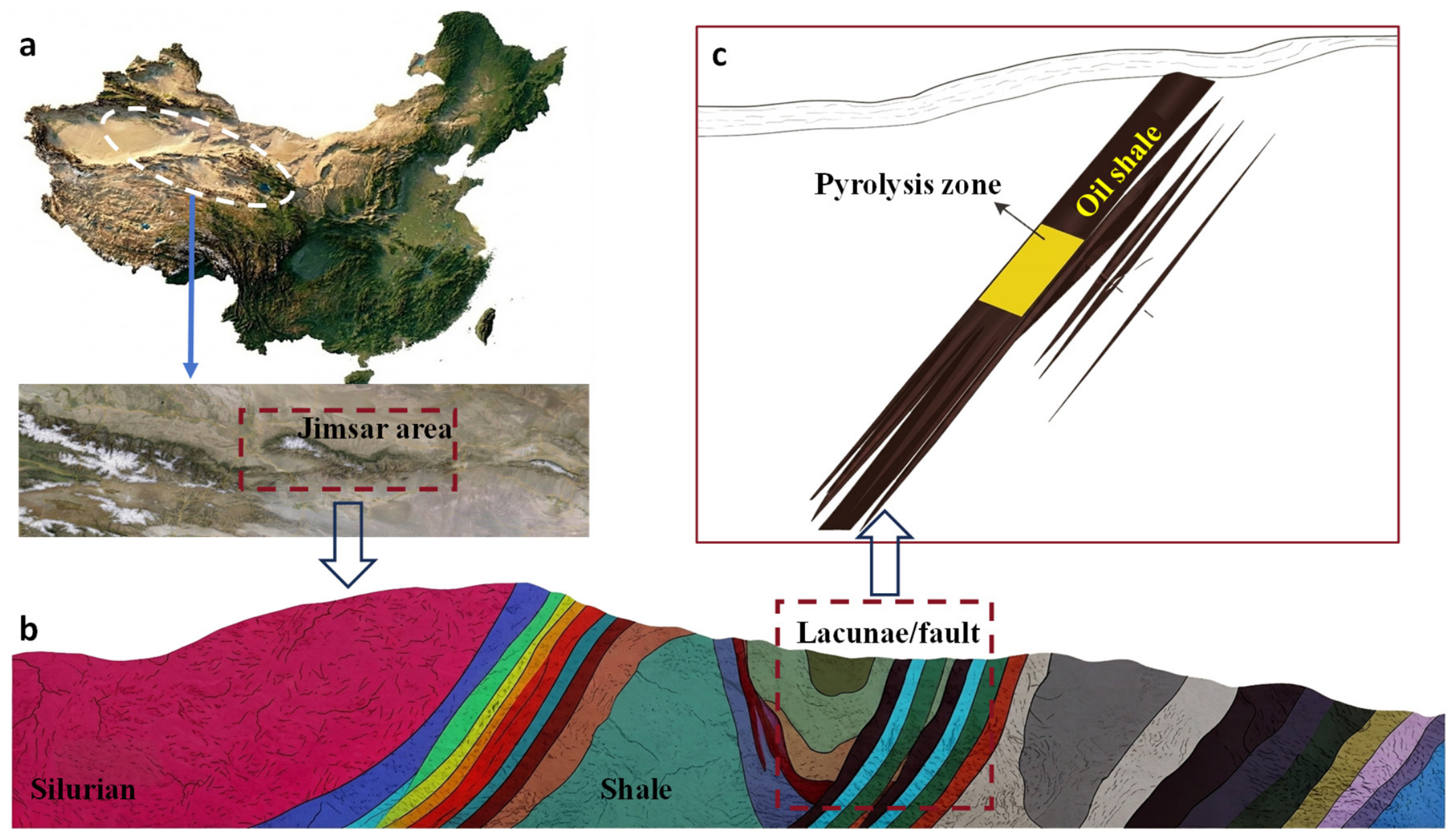
The Jimusar mining area is located at the northern foot of the Bogda Mountains in the Xinjiang Uygur Autonomous Region, China (as shown in Figure 3) [24,25]. The regional tectonic framework consists, from north to south, of the Qitai North Uplift, the Jimusar Sag, the Santai Fault Zone, and the piedmont fold belt of the Bogda Mountains. Influenced by northward thrusting of the Bogda Mountains, the oil shale formations in this area are significantly inclined, with dip angles reaching 60–70°, and individual bed thicknesses ranging from 8 to 70 m. The structural cross-section of the mining area (Figure 3) shows that, within the Lucaogou Formation extending from the piedmont of the Bogda Mountains to the pyrolysis zone, the formation dip increases significantly. This indicates that the piedmont fold belt and fault zones jointly control the occurrence, structural morphology, and spatial distribution of the oil shale reservoir [26,27,28].

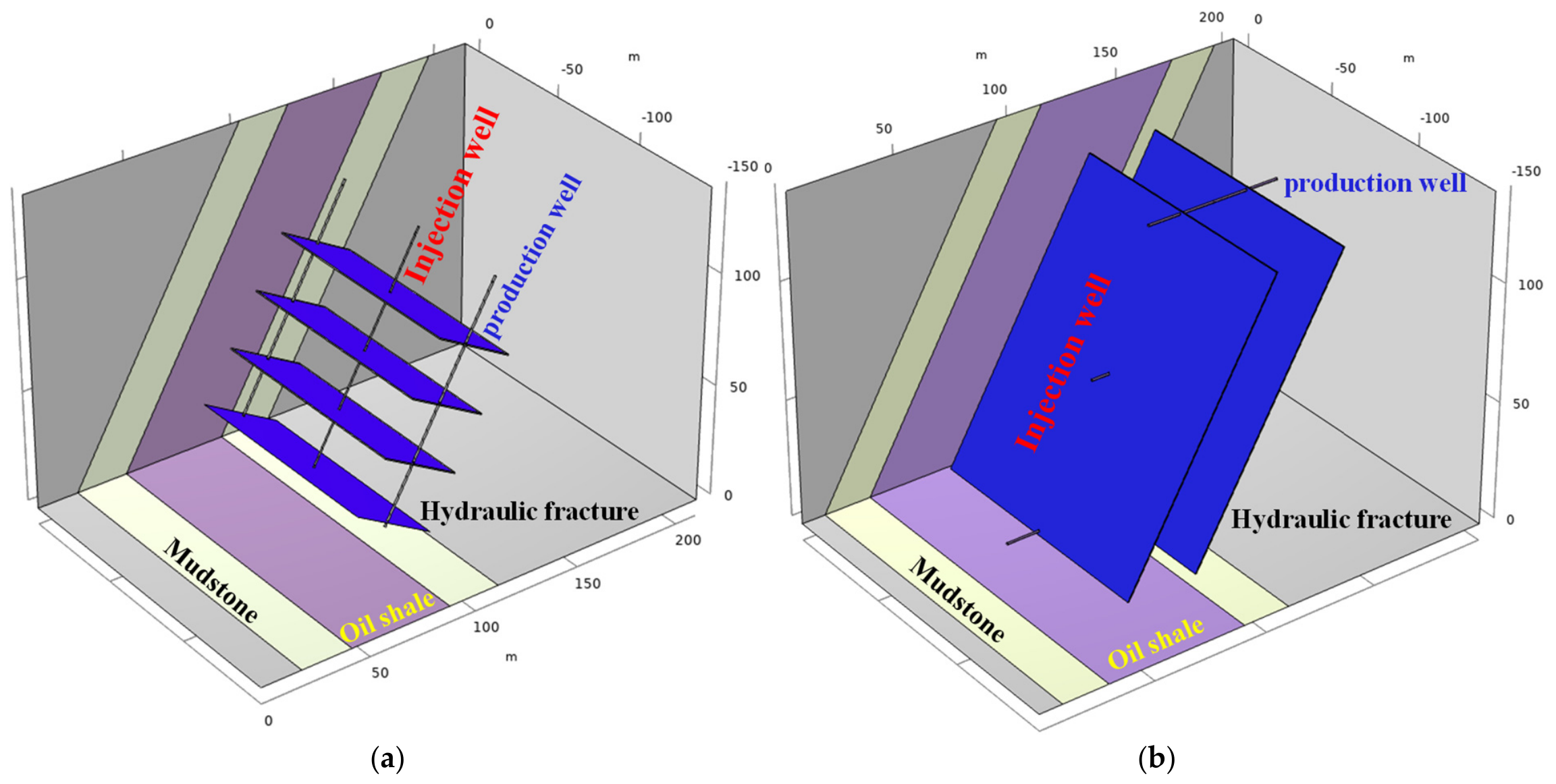
Based on this geological setting, a numerical reservoir model with dimensions of 200 m (length), 150 m (width), and a dip angle of 60° was established. The reservoir thickness was set to 50 m, and the overburden layer was assumed to be sandstone. A previously proposed well arrangement with fracture planes perpendicular to the bedding direction was modified in this study (Figure 4a). Specifically, a new multi-branch well system with fracture planes parallel to the bedding direction was developed (Figure 4b) to improve the heat transfer pathway within the steeply dipping oil shale reservoir. In the proposed well system, auxiliary wells were deployed at different depths extending outward from the main well, forming a vertical arrangement of production well–heating well–production well. The vertical spacing between adjacent auxiliary wells was set to 55 m. After the auxiliary well layout was established, large-scale hydraulic fracturing was conducted in the injection well to generate primary fracture zones. Subsequently, secondary fracturing was performed in the production wells to connect the induced fractures with those generated from the injection well, thereby forming an interconnected fracture network. In the numerical model, the fracture zone thickness was assumed to be 0.5 m. The main well was not explicitly considered in the numerical domain because it primarily serves as a wellbore for connecting and supporting the auxiliary wells, while its direct contribution to reservoir-scale heat transfer is limited. Therefore, it was omitted to simplify the computational model without significantly affecting the evaluation of reservoir heat transfer performance. To investigate the effects of well geometry and fracture characteristics on reservoir performance, the heating well length was set to 16 m, 22.5 m, and 29 m; the inter-well inclination angle was varied from 0° to 90° (0°, 30°, 60°, and 90°); the number of fracture planes ranged from 0 to 3; and the fracture extension length was varied from 50 m to 110 m. Here, the fracture extension length represents the lateral propagation distance of the fracture zone along the reservoir plane, rather than the physical fracture aperture or thickness. These parameter ranges were selected based on the geometric characteristics of the Jimusar oil shale reservoir.

3.2. Well Configuration and Reservoir Model

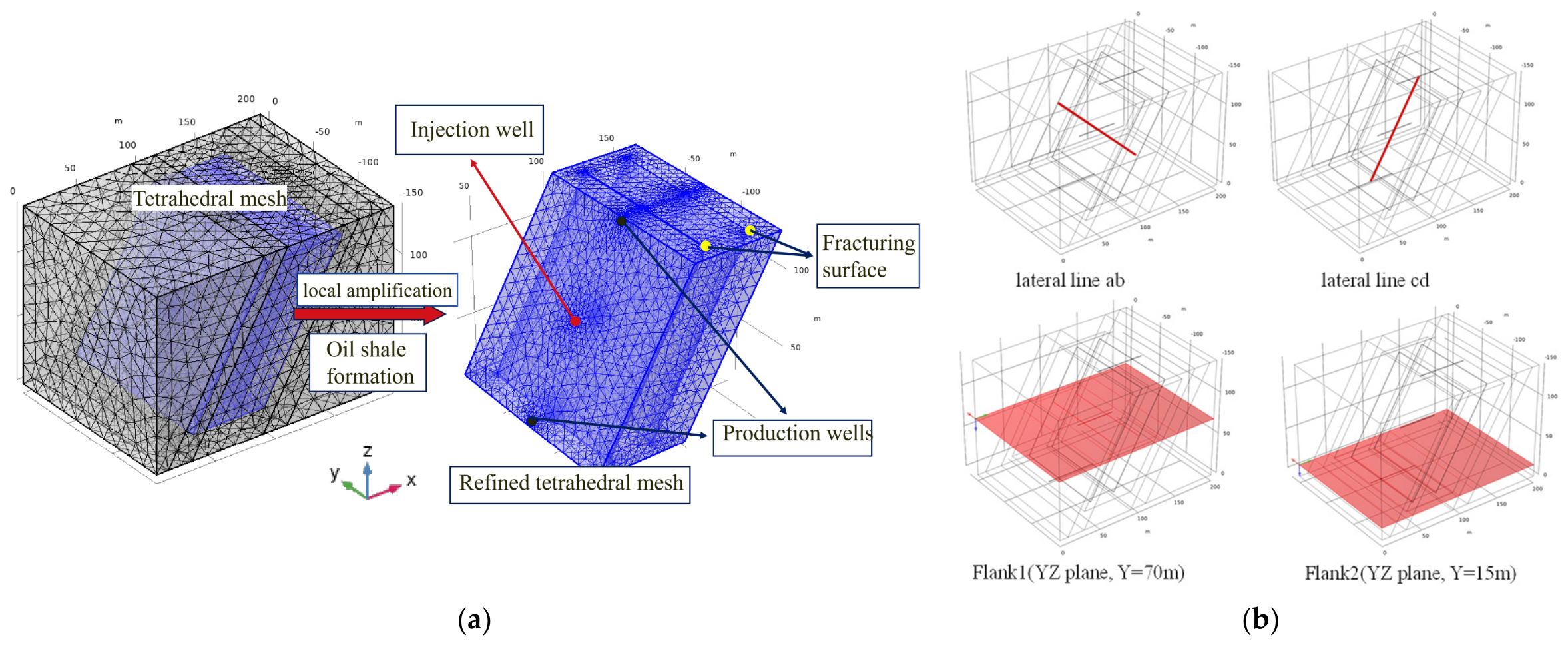
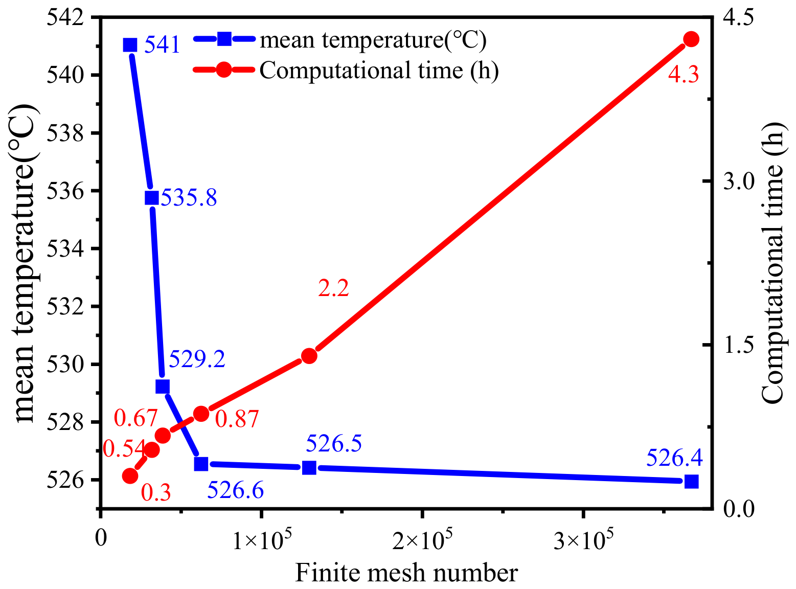
The geometric model was discretized using COMSOL Multiphysics, and the specific simulation scheme is shown in Figure 5a. To capture the strong gradients and coupled multi-physics flow characteristics in the core region of oil shale production between wells, local mesh refinement was applied to ensure numerical accuracy. Meanwhile, multiple data sets such as cut lines and probe surfaces were defined in the model (Figure 5b) to facilitate subsequent multi-dimensional extraction and analysis of simulation results, including temperature and pressure fields. To eliminate the dependence of numerical solutions on spatial discretization, a mesh independence study was conducted by comparing the average reservoir temperature at day 600 under different mesh resolutions (Figure 6). The results indicate that when the number of mesh elements exceeds 129,652, further refinement significantly increases computational cost without notable improvement in accuracy. Considering both numerical accuracy and computational efficiency, an unstructured tetrahedral mesh consisting of 129,652 elements was ultimately selected for subsequent simulations.

3.3. Boundary and Initial Conditions

(1)

The pores of oil shale are initially filled with organic matter. As a result, both porosity and permeability are extremely low at the initial stage; however, these parameters gradually increase with kerogen pyrolysis. Within the heat-affected zone, porosity and permeability are relatively higher. Detailed reservoir anisotropic parameters are provided in Section 3.4.

(2)

Flow field boundary conditions: The initial formation pressure is 0.1 MPa. The injection well is maintained at a constant pressure of 6 MPa, while the production wells are maintained at 0.1 MPa. The injection pressure of 6 MPa was selected based on reported operating conditions for superheated steam-assisted in-situ oil shale conversion and provides a sufficient pressure gradient to sustain steam injection through the low-permeability reservoir without exceeding typical engineering operating conditions. The roof and floor consist of low-permeability mudstone layers, and the upper and lower boundaries are treated as impermeable boundaries [29,30,31,32].

(3)

Temperature field boundary conditions: The initial reservoir temperature is 20 °C, and the injection well temperature is maintained at 600 °C. The injection temperature was selected because it is representative of the superheated steam temperatures commonly adopted in previous in-situ oil shale conversion studies and provides sufficient thermal energy to promote efficient kerogen pyrolysis. All other boundaries are treated as thermally open (free) boundaries [33,34], allowing heat exchange between the computational domain and the surrounding formations. Compared with adiabatic boundaries, this assumption provides a more realistic representation of subsurface heat dissipation. Although some heat loss occurs through the model boundaries, all simulation cases employ identical boundary conditions; therefore, the influence on the comparative evaluation of different well configurations is expected to be limited.

(4)

Chemical field boundary conditions: The initial concentration of kerogen is 200 mol/m³. Additional detailed parameters and numerical settings are shown in

Table 2. Simulation parameters.

Parameters	Variable	Value	Unit	Sources
Oil shale density	ρ	2100	Kg/m3	experiments
Thermal conductivity of oil shale	k	0.5	W/(m·K)	experiments
heat capacity at constant pressure	Cp	1250	J/(kg·K)	experiments
Mixed fluid density	ρf	600	Kg/m3	Ref. [35]
Dynamic viscosity of mixed fluid	μf	1.8 × 10−5	Pa·s	Ref. [35]
Kerogen diffusion coefficient	Dckerogen	0	m2/s	Ref. [36]
Heavy oil diffusion coefficient	DcC25H50	1 × 10−5	m2/s	Ref. [36]
Diffusion coefficient of light oil	DcC9H20	2 × 10−5	m2/s	Ref. [36]
Methane diffusion coefficient	DcCH4	1 × 10−4	m2/s	Ref. [36]
Coke 1/2/3 diffusion coefficient	Dccoke/2/3	0	m2/s	Ref. [36]
Non-hydrocarbon gas diffusion coefficient	Dcgas	1 × 10−4	m2/s	Ref. [36]
The molecular weight of kerogen	Mkerogen	674	g/mol	Ref. [37]
Molecular mass of heavy oil	MC25H50	350.7	g/mol	Ref. [37]
Molecular weight of light oil	MC9H20	128.2	g/mol	Ref. [37]
Molecular mass of methane	MCH4	16.2	g/mol	Ref. [37]
Molecular mass of non-hydrocarbon gases	Mgas	44.0	g/mol	Ref. [37]
Coke 1/2/3 molecular weight	Mcoke/2/3	13	g/mol	Ref. [37]
Initial concentration of kerogen	ckerogen	200	mol/m3	Given

.

3.4. Determination of Anisotropic Reservoir Parameters

(1)

Thermal conductivity [16]:

$${\lambda }_{s-per}=1.176\times {10}^{-6}{T}^2-0.00285T+1.9381$$

(23)

$${\lambda }_{s-par}=4.563\times {10}^{-6}{T}^2-0.00119T+0.7581$$

(24)

where λ_S-per is the thermal conductivity perpendicular to bedding, W/(m·K); λ_S-par is the thermal conductivity parallel to bedding, W/(m·K); and T is the temperature in °C.

(2)

Permeability [16]:

$$k_{per}=\left\{\begin{array}{ll}0\hfill & (20<T<450 °\mathrm{C})\hfill \\ 2.46\times {10}^{-20}T+1.081\times {10}^{-17}\hfill & (450\le T<550 °\mathrm{C})\hfill \\ -2.457\times {10}^{-21}T+2.805\times {10}^{-18}T+7.868\times {10}^{-16}\hfill & (550\le T\le 600 °\mathrm{C})\hfill \end{array}\right.$$

(25)

$$k_{par}=\left\{\begin{array}{ll}-4.539\times {10}^{-22}{T}^2+2.036\times {10}^{-19}T-5.419\times {10}^{-18}\hfill & (20<T<{350 }^{°}\mathrm{C})\hfill \\ 1.759\times {10}^{-20}{T}^2-1.212\times {10}^{-17}T+2\times {10}^{-15}\hfill & (350\le T\le {600 }^{°}\mathrm{C})\hfill \end{array}\right.$$

(26)

where k_per is the permeability perpendicular to the bedding plane, in m²; k_par is the permeability parallel to the bedding plane, in m²; and T is the temperature in °C.

(3)

Porosity [16]:

$$\phi =-5\times {10}^{-7}{T}^3+0.0005T^2-0.1028T+7.2611$$

(27)

3.5. Model Verification

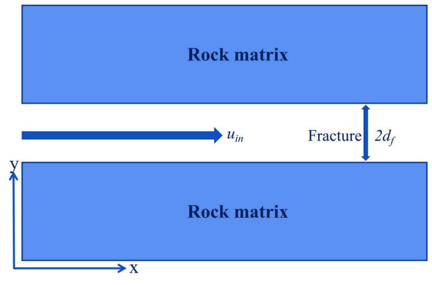
This study employs a precise analytical solution to confirm the reliability of the simulation mode [38]. The schematic representation of this scenario is depicted in Figure 7, illustrating the injection of low-temperature fluid through the entrance of a single 2D fracture. Subsequently, the low-temperature liquid flows through a single fracture to absorb heat from the surrounding matrix, and the heated fluid flows out from the outlet on the right side. Using analytical programs to determine the fluid temperature inside fractures:

$$T_f=T_0+\left(T_{in}^K-T_0\right)erfc\left({\displaystyle \frac{{\lambda }_{s}x/\left({\rho }_f{c}_{f}d\right)}{\sqrt{u_0\left(u_{0}t-x\right){\lambda }_s/\left({\rho }_s{c}_s\right)}}}\right)U\left(t-{\displaystyle \frac{x}{u_0}}\right)$$

(28)

where T_f is the fluid temperature inside the fracture, K; T_in^K is injection temperature of fluid, K; T₀ is the initial temperature of the rock matrix, K; u₀ is injection speed, m/s; t is time; erfc is complementary error function; U is the unit step function. Subsequently, the model was solved using COMSOL software 5.6, and an in-depth exploration of the heat transfer process within the fractures was conducted over a 100-day time frame. The rock matrix in the model is represented as a rectangular structure with a size of 200 × 150 × 50. In

Table 3. Parameters used for model validation.

Parameters	Value
Tin (Injection temperature)	293.15 K
T0 (initial temperature)	423.15 K
Vin (Injection velocity)	0.001 m/s
λr (matrix thermal conductivity)	3 (W/(m·K))
ρr (matrix density)	3000 kg/m3
ρw (water density)	1000 kg/m3
Cr (matrix heat capacity)	1000 J/(kg·K)
Df (fracture aperture)	0.001 m

, the input parameters for the numerical and analytical models are listed.

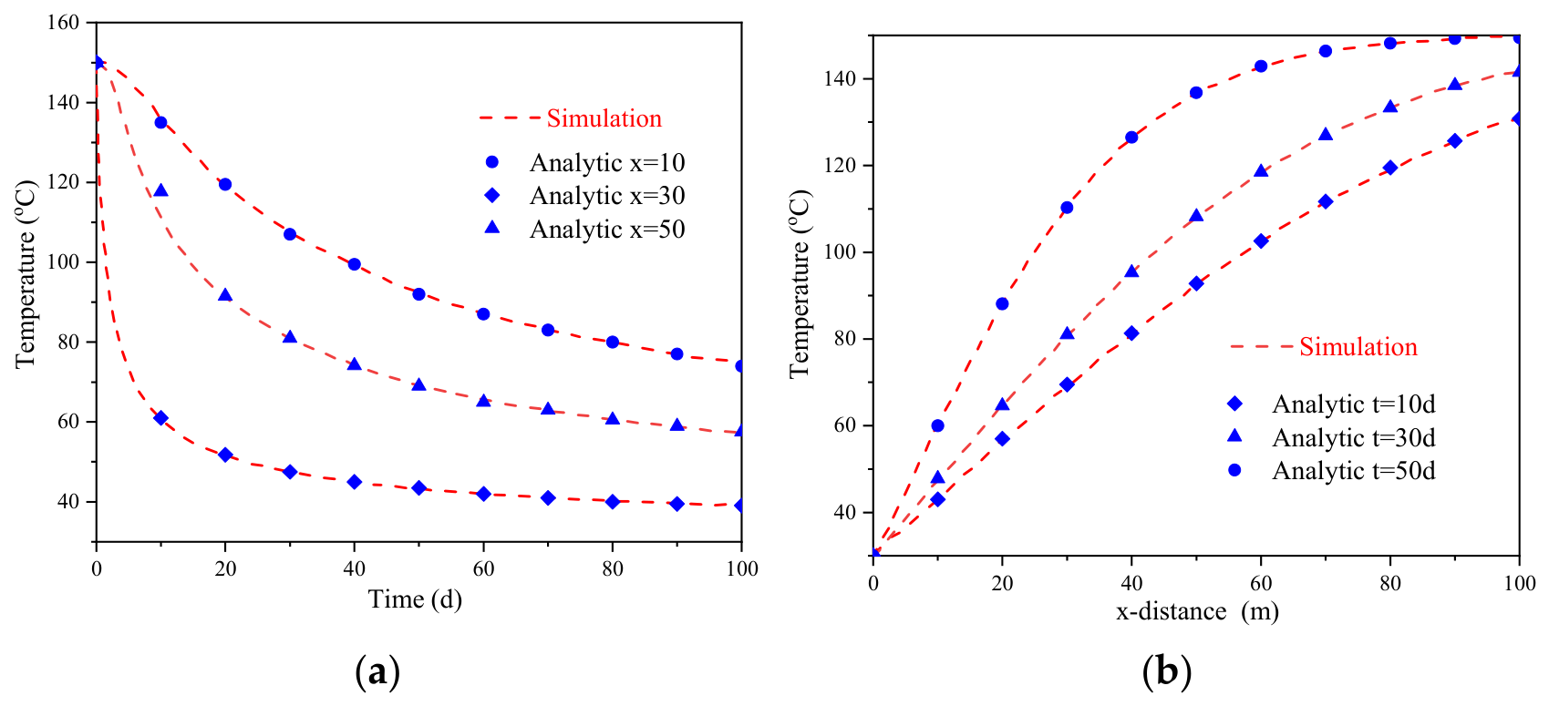
A comparison between the analytical and the numerical solutions is performed in Figure 8, where Figure 8a shows fractures at different locations with temperature changes over time (x = 10 m, 20 m, 30 m), and Figure 8b displays fractures with temperature distribution patterns at different times (t = 10 d, 30 d, 50 d). It is clear that the two solutions are highly consistent, with only a slight difference. Although the chemical reaction field was not validated independently because no analytical solution is available, the pyrolysis process is governed by established temperature-dependent kinetic equations. Since the reaction rate is directly controlled by the simulated temperature field, the validated thermal model provides a reliable basis for predicting the thermo-chemical conversion behavior. All in all, this shows that the numerical model used to simulate the complex process of coupled fluid flow and heat transfer is highly reliable and very suitable for the study of oil shale mining.

4. Performance Analysis of the Proposed Multi-Branch Well System

4.1. Evolution of Pressure, Velocity and Temperature Fields

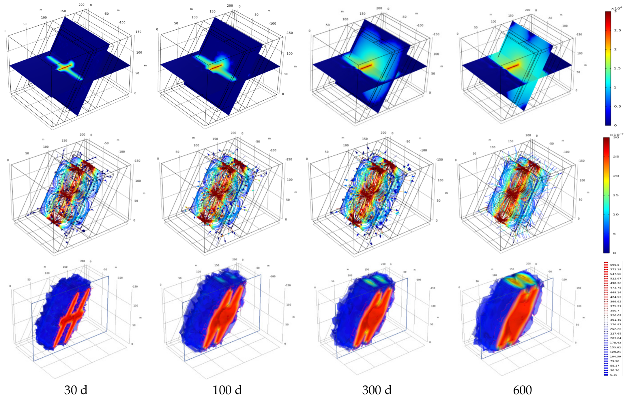
Figure 9 illustrates the temporal evolution of injection pressure, flow rate, and temperature in the reservoir during the injection process. As shown in the first row of Figure 9 in the early injection stage, the injected superheated steam preferentially enters the fracture network, where a stable pressure gradient is first established within the fractures. Due to the higher permeability along the bedding direction of oil shale, steam predominantly flows parallel to bedding, while the low permeability in the perpendicular direction can be mitigated by optimizing fracture spacing and number. As shown in the second row of Figure 9, the flow velocity is relatively high in the reservoir surrounding the injection well and within the fracture system. At the connection region between the injection and production wells, the steam velocity increases significantly due to the large pressure gradient. In contrast, in other regions, the flow rate remains relatively low owing to smaller pressure gradients. As shown in the third row of Figure 9, high-temperature zones first develop rapidly around the fractures and the injection well, and then progressively expand outward with increasing injection time. This is attributed to the continuous migration of high-temperature steam from the injection well toward the surrounding reservoir, which gradually enhances the steam transport pathways within the oil shale formation. It is noteworthy that, due to the anisotropy of permeability in oil shale, the thermal diffusion rate along the bedding direction is significantly higher than that in the perpendicular direction. Over time, the high-temperature regions generated by the two fracture planes gradually merge. At 600 days of injection, the temperature of most reservoirs exceeds 500 °C, but the temperature at the upper and lower production wells does not reach 500 °C, which indicates that most of the oil shale thermal conversion can be achieved at this time point, but there is still a small part of the area that is not pyrolyzed or the degree of pyrolysis is low.

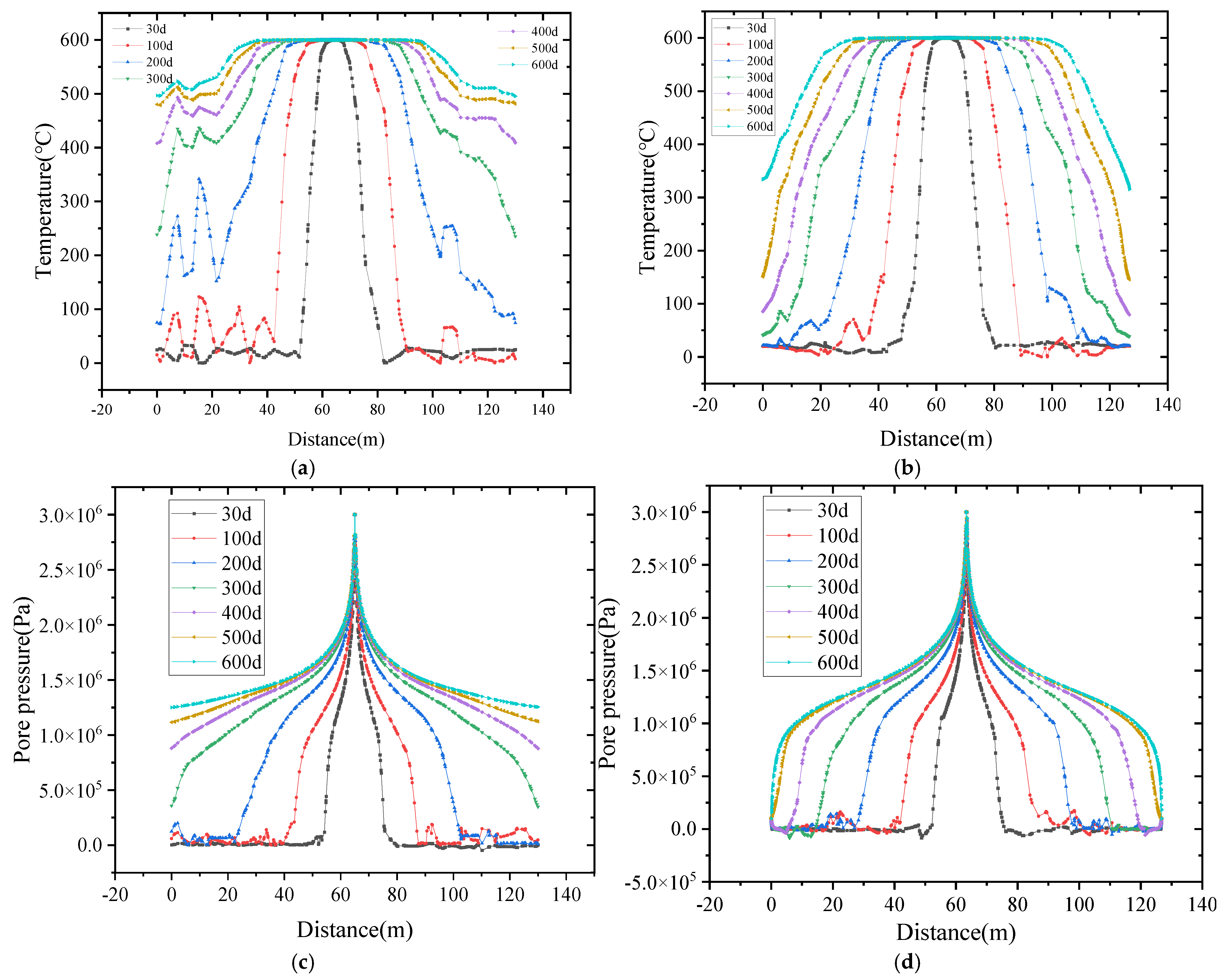
Figure 10 presents the temporal distributions of pressure and temperature along lines ab and cd at different times. Both lines are located between two fracture zones and are mutually perpendicular, as clearly marked in Figure 5b. Figure 10a,b illustrate the temperature evolution along these two profiles. At 30 days of heating, only a zone of approximately 5 m around the fractures reaches temperatures of about 500 °C. When the heating duration extends to 600 days, the temperature along the ab direction is generally above 500 °C. For the cd direction, most of the region between the injection and production wells also exceeds 500 °C; However, the temperature near the production well drops sharply to near the initial reservoir temperature. This is because high-temperature fluids are continuously extracted together with the produced fluids before sufficient heat can be transferred to the surrounding oil shale. Consequently, the temperature in the vicinity of the production well remains relatively low, resulting in incomplete kerogen pyrolysis and limited enhancement of porosity and permeability. This, in turn, restricts steam migration and the transport of generated hydrocarbons toward the production well, thereby reducing local production efficiency. Figure 10c,d show the pore pressure distributions along the two profiles. As heating progresses, the overall pore pressure gradually increases throughout the reservoir. However, a pronounced pressure decline develops near the production well along profile cd. Combined with the temperature distribution, this indicates that the relatively low temperature limits kerogen conversion and the associated permeability enhancement, leading to restricted fluid flow and the formation of a localized low-pressure zone. During the production process, an appropriate arrangement of production wells can intentionally maintain this localized low-temperature and low-pressure zone at the boundary of the production area. This boundary helps reduce heat dissipation from the heated reservoir to the surrounding formations, thereby improving thermal utilization efficiency and mitigating the thermal disturbance to adjacent strata.

4.2. Comparison with Conventional Well Arrangement

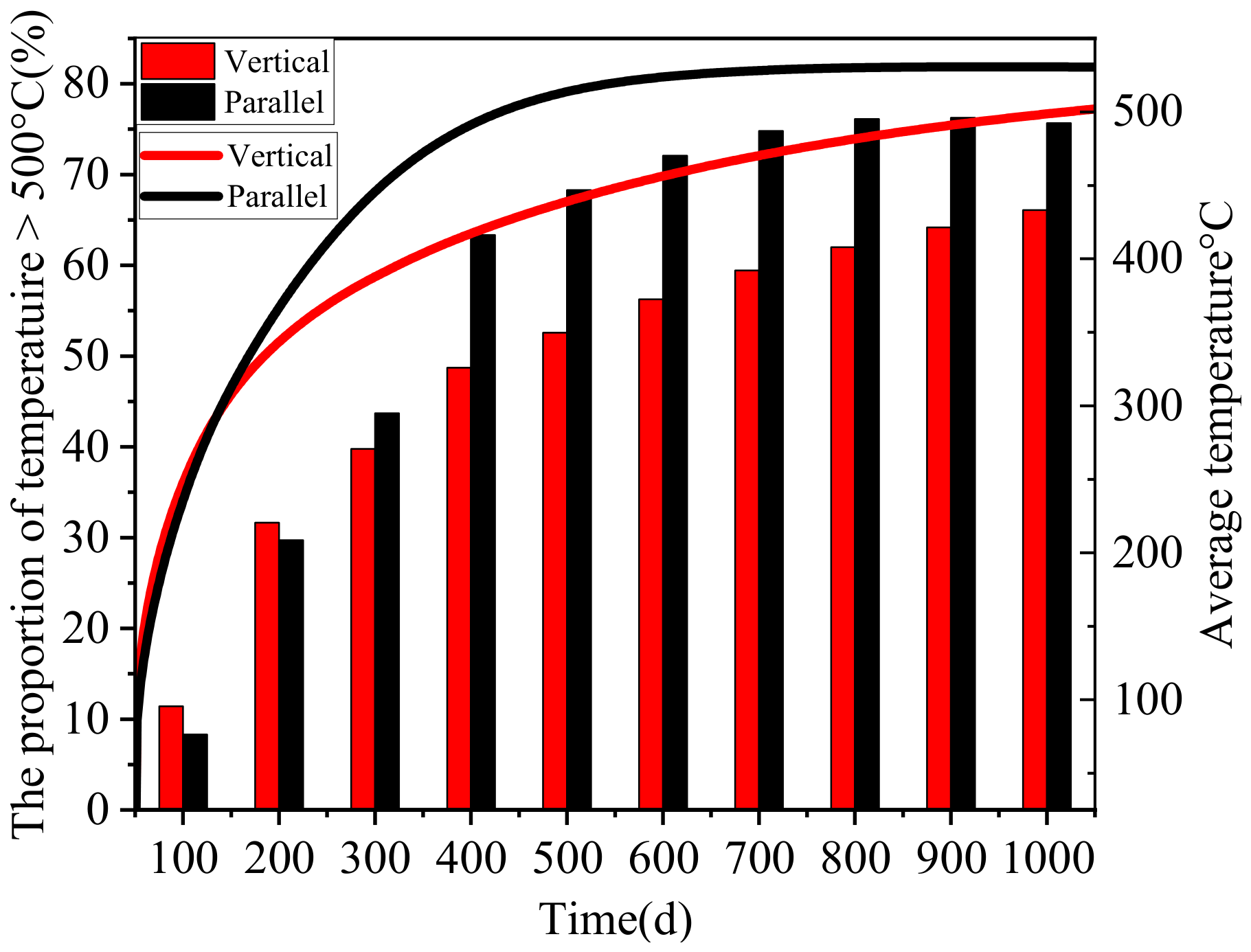
This section compares the heat transfer performance and initial investment cost of two well layout schemes with different wellbore orientations. Scheme 1 (The fracturing surface is parallel to the bedding direction), whereas in Scheme 2 (The fracturing surface is vertical to the bedding direction). Figure 11 presents the comparison of the average reservoir temperature (bar chart) and the proportion of the high-temperature region (line chart) for the two schemes. The results indicate that, during the early stage of heating, Scheme 2 exhibits a higher average reservoir temperature than Scheme 1. However, as heating progresses, the average temperature of Scheme 1 gradually exceeds that of Scheme 1 and approaches a stable value after approximately 800 days, indicating that the reservoir has nearly reached thermal equilibrium. In contrast, Scheme 2 continues to exhibit a gradual temperature increase. The line chart further shows that the proportion of the high-temperature region in Scheme 1 surpasses that in Scheme 2 at approximately 200 days and remains nearly constant after 600 days. It shows that the effective pyrolysis zone has reached the maximum range. These results show that compared with the vertical bedding, setting the direction of the fracturing surface parallel to the strike of the rock layer can significantly improve the heat transfer efficiency and expand the effective pyrolysis area.

In practical engineering applications, the superiority of a given scheme cannot be evaluated solely based on heat transfer efficiency or pyrolysis efficiency; instead, a comprehensive assessment is required. Accordingly, the initial cost of each scheme can be calculated using Equation (29) [16], enabling a quantitative comparison of the economic performance of different well layouts.

$$C_f=n_f\times 800\times L_{tp}^{0.9}+n_w\times 330\times L_w+n_w\times 50\times t$$

(29)

where C_f is the Drilling, fracturing costs, and operation and maintenance costs, $; n_f is the fracture number; L_tp is the length of the fracture, m; n_w is the well number; L_w is the length of the well, m; and t is the operation of the injection system, d.

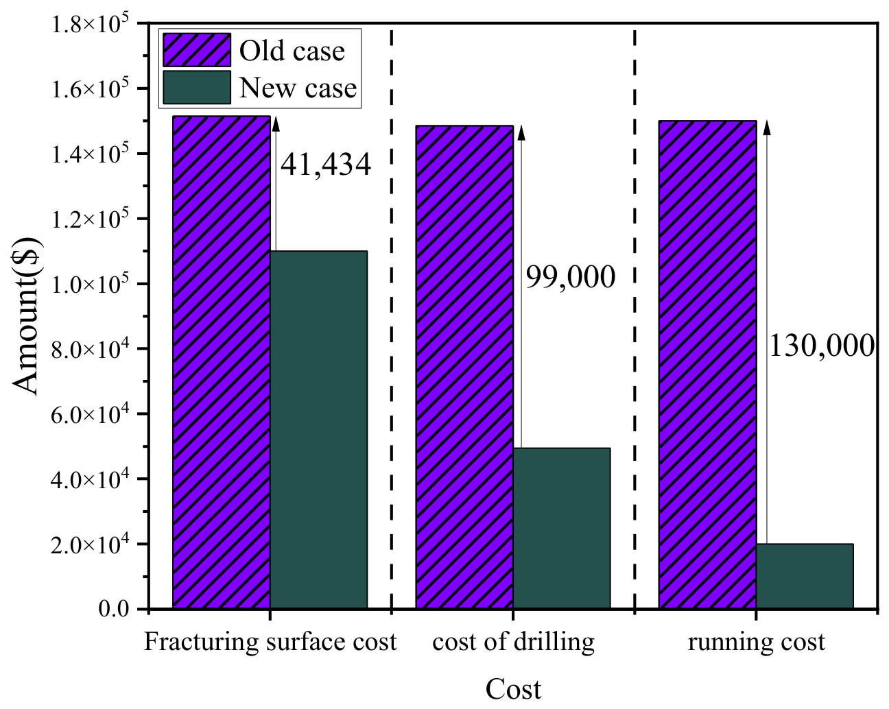
Figure 12 shows the initial cost composition of the two schemes, including fracturing cost, drilling cost, and operation cost. The specific parameters are shown in

Table 4. The specific parameters of the two schemes.

	Running Time (Days)	Fracturing Surface Width (m)	Number of Fracturing Surfaces	Number of Main Wells	Data Sources
scheme 1	400	110	2	1	simulation
scheme 2	1000	72.6	4	3	Ref. [16]

. The results show that Scheme 1 has lower costs than Scheme 2 in all three categories. This economic advantage is mainly attributed to Scheme 1, which enhances heat-transfer efficiency and reservoir conversion performance while reducing the required operation duration. Consequently, the proposed configuration decreases the overall investment associated with drilling, fracturing, and long-term operation. Considering both thermal performance and economic feasibility, the proposed configuration demonstrates better engineering applicability for in-situ oil shale conversion. Therefore, this configuration is selected for subsequent analysis, where the effects of key operational parameters on reservoir performance are further investigated.

5. Parametric Analysis of Key Engineering Factors

5.1. Effect of Heating Well Length

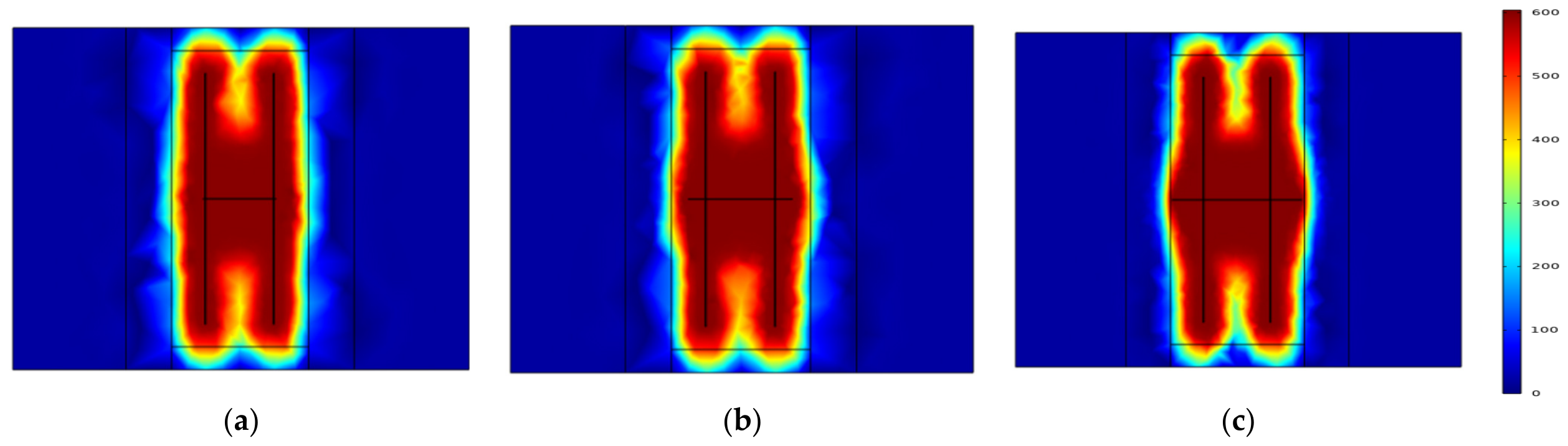
Figure 13 shows the temperature contour maps of a cross-section at a height of 75 m under different injection well lengths at 300 days. Apart from the significant differences at both ends of the heating well, the temperature distributions in other regions are generally consistent. Overall, as the length of the heating well increases, the high-temperature zones at both ends become more pronounced. When the heating well length reaches 29 m, the high-temperature regions at both ends have already extended into the overburden after 300 days. This phenomenon indicates a clear drawback: after 300 days, heat conduction at both ends of the heating well becomes ineffective heat transfer, leading to unnecessary energy loss. Therefore, relying solely on qualitative observation of temperature contour maps is insufficient to determine the optimal condition. A quantitative analysis is required to evaluate and compare the performance under different configurations.

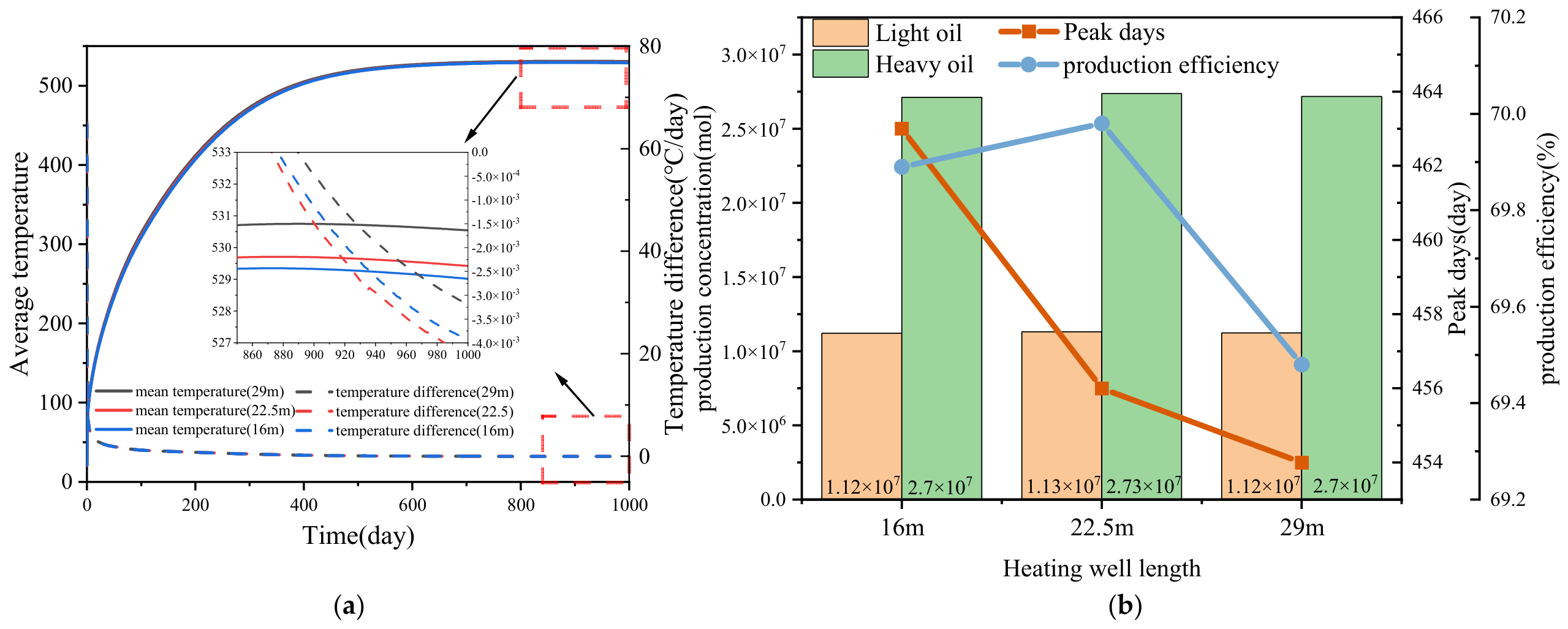
Figure 14 illustrates the temporal evolution of the reservoir average temperature and the daily temperature change under different heating well lengths. As shown in Figure 14a, the curves of average temperature and daily temperature increment under the three cases are nearly identical, indicating that the overall heat transfer efficiency is almost the same under different heating well lengths. From the partially enlarged view of the later stage, it can be observed that the average reservoir temperature slightly increases with increasing heating well length; however, the difference is very small, approximately within 0.5–1 °C. The enlarged view of the daily temperature change further shows that when the temperature difference approaches zero, it indicates that the reservoir has reached thermal equilibrium. It is noteworthy that a longer heating well length does not necessarily lead to an earlier equilibrium time. Instead, the earliest equilibrium is observed when the heating well length is 22.5 m, followed by 16 m, while the 29 m case reaches equilibrium the latest. This further demonstrates that increasing heating well length does not continuously enhance heat transfer efficiency; excessively long heating wells may instead lead to energy waste. Figure 14b presents the peak production time, peak light oil and heavy oil yields, and oil shale conversion efficiency under different heating well lengths. The bar chart shows that the differences in light and heavy oil production among the three cases are very small; however, under the 22.5 m condition, both light oil and heavy oil yields are approximately 200,000 mol higher than those of the other cases. The line chart indicates that the peak production time shifts slightly earlier with increasing heating well length, but the difference is within 10 days. The oil shale conversion efficiency reaches its maximum value of approximately 70% under the 22.5 m condition. Within the parameter range considered in this study, the 22.5 m case demonstrates the best overall performance in terms of comprehensive development efficiency.

5.2. Effect of Heating Well Angle

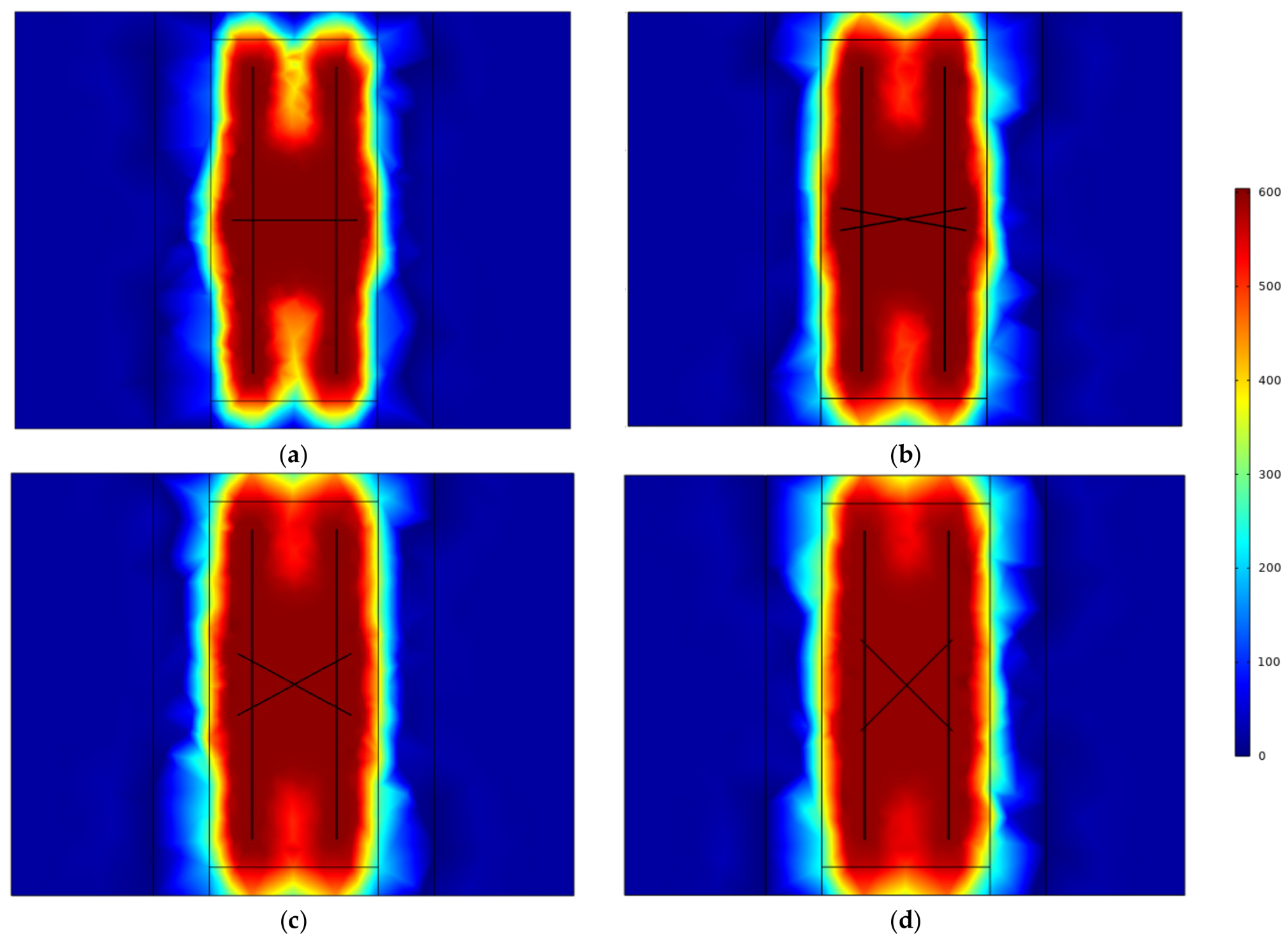
Figure 15 shows the temperature distribution of the oil shale reservoir at 300 days on Section 1 (location shown in Figure 5b) under four different heating well intersection angles. When the heating well angle is 0°, obvious depressions appear at both ends of the high-temperature region, and low-temperature underheated zones exist at the top and bottom boundaries. As the heating well angle increases to 30°, 60°, and 90°, the vertical heat diffusion capability between wells is continuously enhanced. The contour of the high-temperature region becomes increasingly complete and regular, while the low-temperature blind zones at the upper and lower boundaries gradually disappear, indicating improved heating uniformity of the reservoir. In the 90° cross-layout case, the high-temperature coverage between wells is the largest and the temperature field is the most uniform. This suggests that increasing the intersection angle of heating wells can optimize steam heat-transfer pathways, enhance vertical heat conduction within the reservoir, and expand the effective pyrolysis zone.

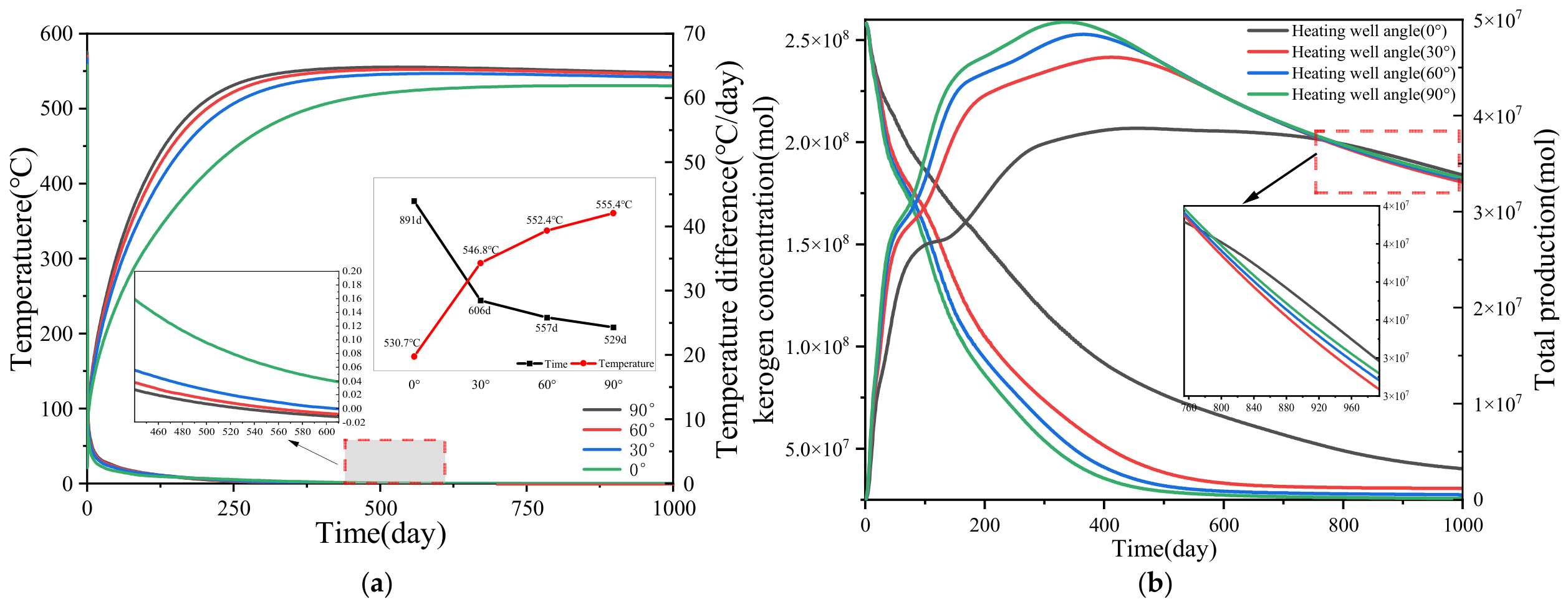
Figure 16a presents the average reservoir temperature, daily temperature variation, equilibrium temperature, and the time required to reach thermal equilibrium under different inter-well angles. By combining the main plot and inset, it can be observed that the temperature evolution under all cases follows a consistent three-stage pattern, namely “heating stage–quasi-steady stage–thermal equilibrium stage”. However, significant differences exist in both the rate of reaching thermal equilibrium and the final equilibrium parameters. The main plot indicates that as the inter-well angle increases from 0° to 90°, the overall average reservoir temperature gradually rises and enters the quasi-steady state earlier. In the early stage, the temperature increase rates are relatively similar among different cases, while noticeable divergence appears in the middle and late stages. Ultimately, the 90° case achieves the highest average temperature (approximately 555 °C), whereas the 0° case exhibits the lowest value (approximately 530 °C). The inset further reveals the key characteristics at the thermal equilibrium point for each case. The time required to reach thermal equilibrium decreases from 891 days (0°) to 529 days (90°), while the corresponding equilibrium temperature increases progressively from 530.7 °C to 555.4 °C. The underlying mechanism is that a larger inter-well angle improves the spatial connectivity of the fracture network and optimizes the three-dimensional distribution of steam within the reservoir. This promotes more uniform heat transfer and fluid transport in both the lateral and vertical directions under the influence of reservoir anisotropy, resulting in more efficient volumetric heating. In contrast, under small inter-well angles, steam preferentially migrates along the bedding planes, leading to uneven heat distribution, slower heat propagation throughout the reservoir, delayed thermal equilibrium, and lower final equilibrium temperatures. Therefore, these results demonstrate that the inter-well angle is a key structural parameter controlling the three-dimensional heat transfer behavior, thermal evolution rate, and final equilibrium state of the reservoir.

Figure 16b illustrates the evolutionary characteristics between kerogen consumption and oil generation during the in-situ pyrolysis process. The kerogen concentration does not approach complete depletion until approximately 500–600 days, whereas the peak oil and gas production occurs much earlier, at around 300–400 days. This indicates that production behavior is not solely controlled by the degree of kerogen conversion but is significantly influenced by the overall thermal evolution of the reservoir. During the early to mid pyrolysis stage, as reservoir temperature continuously increases and exceeds the kerogen pyrolysis threshold, a large amount of kerogen is decomposed, resulting in a rapid increase in hydrocarbon production. With continued heating, high-temperature zones gradually develop within the reservoir, particularly near the wellbore region. At this stage, although residual kerogen still exists, the previously generated heavy hydrocarbons begin to undergo secondary fracturing, further converting into light gases such as methane, while part of the organic matter is transformed into coke through condensation reactions. Meanwhile, the remaining kerogen continues to decrease, and the primary generation rate of oil gradually declines. Under the combined effects of intensified secondary fracturing and depletion of kerogen supply, oil and gas production reaches its peak before complete kerogen exhaustion and then begins to decline. Overall, as the inter-well angle increases, the high-temperature coverage becomes more extensive. The 90° case exhibits more uniform temperature distribution and a higher degree of kerogen conversion, indicating improved overall pyrolysis efficiency.

5.3. Effect of Hydraulic Fracture Number

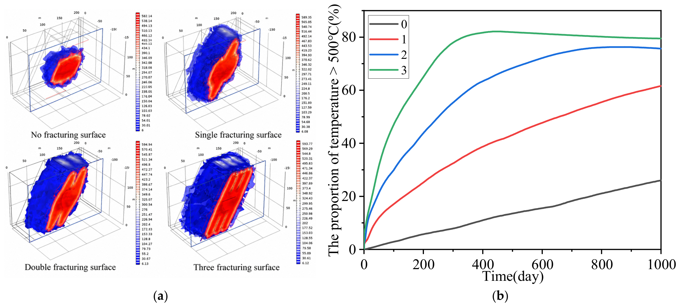
Figure 17 illustrates the spatial extent of the core thermal zone within the reservoir, defined as regions with temperatures exceeding 500 °C, under different numbers of fracturing planes. The results clearly indicate that, in the absence of any fracture planes, the high-temperature region is confined to the vicinity of the wellbore, resulting in a very limited affected volume. As the number of fracture planes increases, the high-temperature isotherms expand significantly along the fracture channels, and the affected volume increases in a near-exponential manner. In the case with three fracture planes, the high-temperature zone achieves efficient and relatively uniform coverage of the entire production area. This strongly demonstrates that increasing the number of fracture planes can effectively overcome the low-permeability limitation of oil shale.

Figure 17b quantitatively characterizes the evolution of the area fraction of the high-temperature region (T > 500 °C), which reflects the overall reaction degree of kerogen in the reservoir during in-situ pyrolysis. In the case without fracture planes (black curve), the expansion of the high-temperature pyrolysis zone is severely constrained by the low permeability of the reservoir. Even after 1000 days of heating, the area fraction of the region exceeding 500 °C is only about 25%, indicating that most kerogen has not yet reached effective thermal decomposition conditions and the overall conversion degree of the reservoir remains low. In contrast, the introduction of fracture planes significantly improves heat transfer conditions and promotes rapid outward propagation of the pyrolysis front. Among all cases, the three-fracture-plane configuration (green curve) exhibits the highest thermal efficiency, with the pyrolysis area fraction rapidly increasing to over 80% within approximately 400 days, indicating that most of the reservoir has reached high-efficiency pyrolysis conditions. After this stage, the curve stabilizes with a slight decline, suggesting that kerogen in the core region has been largely depleted and the system gradually enters a late-stage heat-maintenance regime. Although the two-fracture-plane case (blue curve) shows a similar evolution trend, it requires approximately 800 days to reach a pyrolysis area fraction of about 75%, indicating a significantly slower propagation rate compared with the three-fracture-plane scenario. Overall, increasing the number of fracture planes effectively enhances heat transfer and thermal diffusion within the reservoir, accelerates pyrolysis kinetics, and expands the coverage of the high-temperature zone. This substantially shortens the time required for large-scale kerogen conversion and improves the development efficiency of low-permeability oil shale reservoirs.

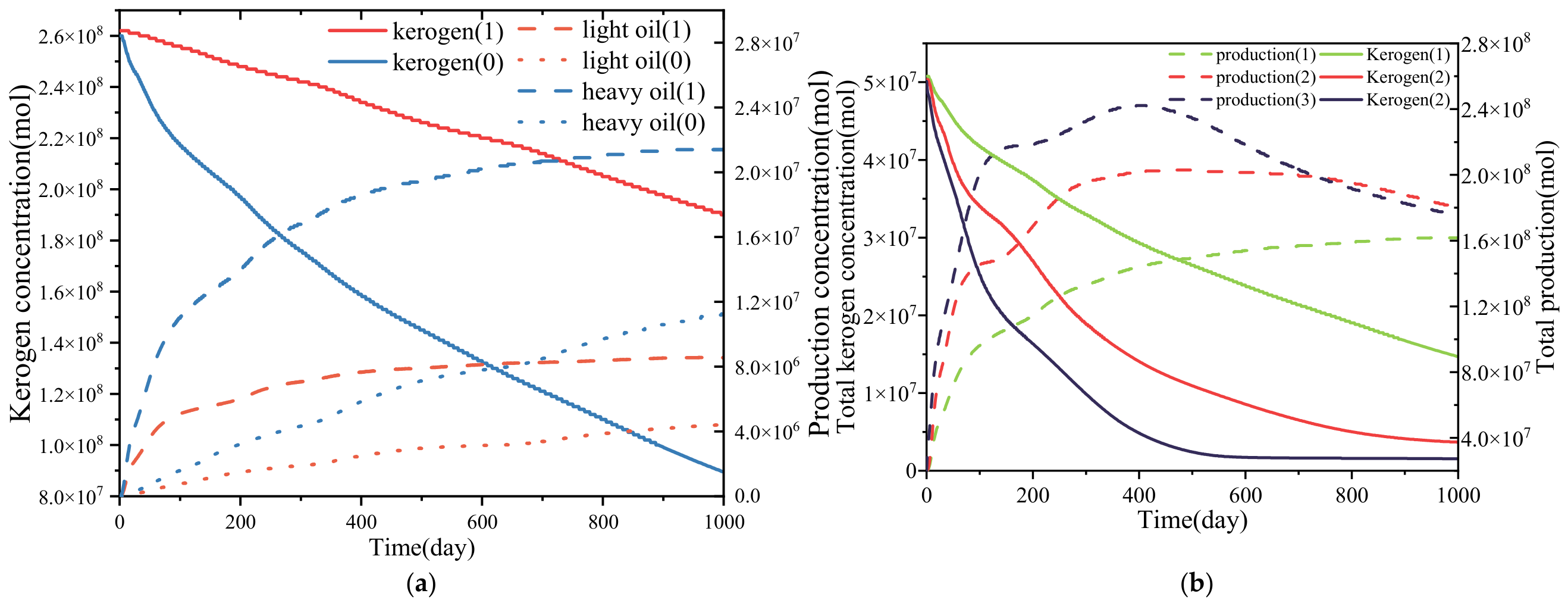
Figure 18a illustrates the temporal evolution of kerogen consumption and cumulative oil product generation under conditions with fractures (1) and without fractures (0). Overall, the continuous depletion of kerogen shows a clear correspondence with the accumulation of heavy oil and light oil; however, significant differences in conversion efficiency are observed between the two cases. First, regarding kerogen evolution, the kerogen concentration in both cases continuously decreases with time, indicating ongoing pyrolysis reactions within the reservoir. However, the depletion rate under fractured conditions is markedly higher than that under the non-fractured case. By 1000 days, the remaining kerogen under the fractured condition decreases to approximately (9.0 × 10⁷) mol, whereas it remains at about (1.9 × 10⁸) mol without fractures. This demonstrates that the introduction of fracture planes significantly enhances reservoir heat transfer, enabling a larger volume of the formation to reach the temperature required for kerogen pyrolysis. As a result, the pyrolysis front advances more rapidly into deeper regions, leading to a higher overall conversion degree of kerogen. The large-scale decomposition of kerogen directly promotes the generation of hydrocarbon products. As shown in Figure 18a, heavy oil production is consistently higher than light oil production in both cases, indicating that kerogen initially generates heavy oil as the dominant product under the current pyrolysis conditions. By 1000 days, the cumulative heavy oil production under the fractured condition reaches approximately (2.1 × 10⁷) mol, compared with only (1.2 × 10⁷) mol in the non-fractured case, representing an increase of about 75%. Meanwhile, light oil accumulation increases from approximately (4.5 × 10⁶) mol in the non-fractured case to about (8.5 × 10⁶) mol in the fractured case, corresponding to an increase of nearly 90%.

Figure 18b illustrates the temporal evolution of remaining kerogen and cumulative oil production under different numbers of fracture planes. As the number of fracture planes increases, the kerogen depletion rate is significantly accelerated. In the three-fracture-plane case, pyrolysis is nearly completed at approximately 600 days, whereas in the single-fracture-plane case, a substantial amount of unreacted kerogen remains even at 1000 days. Correspondingly, oil production in all cases shows a typical trend of initial increase followed by stabilization and even decline. The three-fracture-plane configuration achieves the highest production peak, reaching approximately (4.7 × 10⁷) mol, with the peak occurring earlier than in other cases. The two-fracture-plane case reaches a peak of about (3.8 × 10⁷) mol, while the single-fracture-plane case shows a continuously slow increase without a distinct peak within the simulated period. It is noteworthy that both the two- and three-fracture-plane cases exhibit a decline after reaching their peak values. This indicates that, in the late stage, the rate of secondary fracturing of hydrocarbons gradually exceeds the rate of hydrocarbon generation. As a result, a significant portion of heavy and light oils is further converted into gaseous products and semi-coke. Overall, increasing the number of fracture planes expands the steam sweep volume and significantly enhances kerogen conversion efficiency, thereby increasing oil yield. However, excessive fracture development may also lead to rapid local temperature rise, which promotes secondary fracturing of previously generated liquid hydrocarbons into lighter gases and coke. Therefore, although increasing fracture plane number improves pyrolysis efficiency, it may reduce the preservation efficiency of liquid hydrocarbons in the later stage.

5.4. Effect of Hydraulic Fracture Width

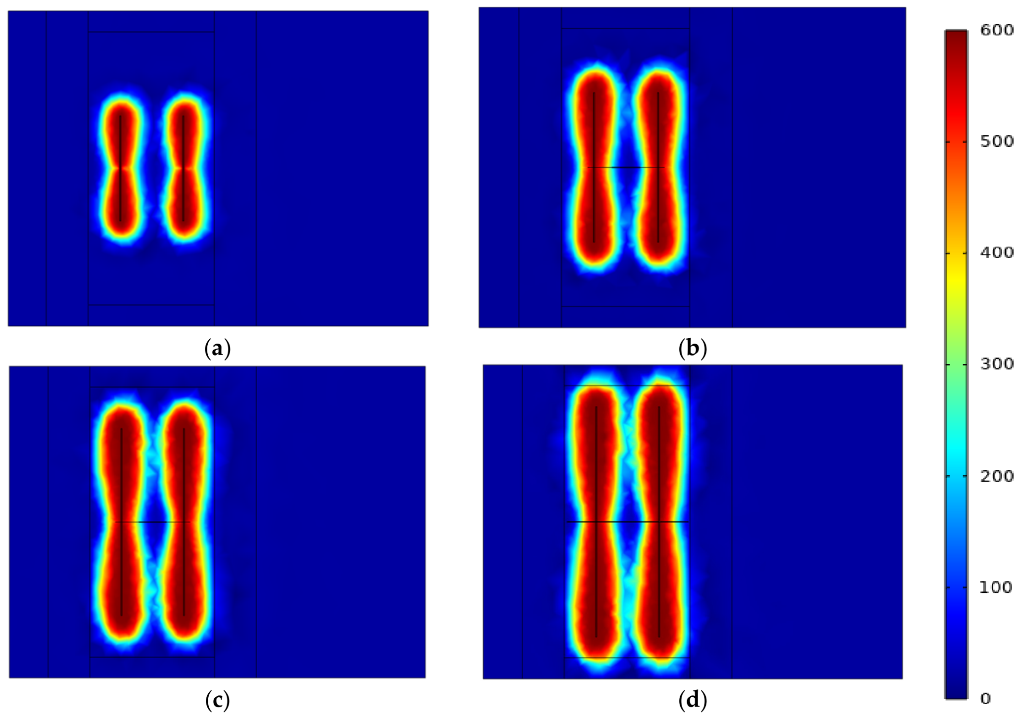
Figure 19 shows the temperature distribution characteristics on the cross section of 2 (as shown in Figure 5b) under different fracture widths after heating for 300 days. As the fracture width increases from 50 m to 90 m, the high-temperature region continuously expands, and the thermal influence zones on both sides gradually strengthen and tend to become connected. This indicates that the fracture network significantly enhances the heat transfer capacity of the reservoir, thereby improving overall heating uniformity and accelerating the propagation of the pyrolysis front. However, a distinct low-temperature zone still exists in the middle of the measurement line. This phenomenon is mainly attributed to the converging effect of the production well, where the fluid rapidly flows toward the wellbore and is produced, resulting in reduced residence time and weakened convective heat transfer, which suppresses local temperature increase. In addition, when the fracture width is further increased, part of the heat is dissipated into the overlying and underlying formations, leading to additional ineffective heat loss. Overall, increasing fracture width can significantly improve reservoir heating performance; however, excessive widening may intensify flow convergence cooling and boundary heat losses, thereby reducing local thermal utilization efficiency.

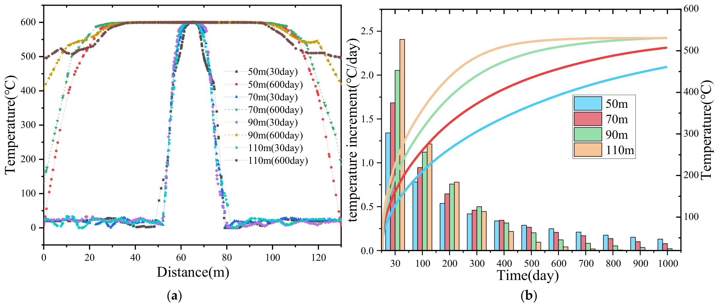
Figure 20a shows the temperature distribution characteristics along line (ab) at 30 days and 600 days under different fracture-width conditions. At the early heating stage (30 days), the temperature fields under all cases are nearly identical, indicating that due to the ultra-low permeability and strong anisotropy of oil shale, heat transfer is dominated by conduction, and the influence of fracture scale is not yet significant. As heating proceeds to 600 days, the overall reservoir temperature increases substantially, while differences among cases gradually emerge. Under the 50 m fracture-width condition, the temperature in approximately 20 m regions at both ends of the profile remains below 500 °C, indicating the presence of under-heated zones, with an estimated unreacted fraction of about 28%. In contrast, when the fracture width increases to 110 m, the temperature along the entire profile exceeds 500 °C, suggesting that the reservoir has essentially achieved complete thermal conversion. Figure 20b presents the evolution of daily average temperature increase (bar chart) and average reservoir temperature (line chart) under different fracture-width conditions. The results show that all cases experience a similar two-stage evolution process, consisting of a rapid heating stage followed by a gradual stabilization stage. In the early stage (within approximately 10 days), the average temperature curves of all cases nearly overlap, and differences in daily temperature increment are minimal, indicating that heat transfer is mainly controlled by matrix conduction, and the effect of fracture width is negligible. As time progresses, significant divergence among different cases becomes apparent. The average reservoir temperature increases with increasing fracture width. The 110 m case exhibits the most pronounced heating performance, reaching approximately 500 °C across the reservoir at around 600 days, whereas the 50 m case remains limited by restricted flow capacity, leaving a relatively large low-temperature region and lower pyrolysis degree. The bar chart further indicates that, under the same heating duration, the daily temperature increment increases with fracture width. This is because wider fracture planes provide larger fluid transport and heat exchange pathways, enabling more heat to be delivered into the reservoir and thus enhancing the overall heating rate. However, as the heating process continues, the daily temperature increment in all cases gradually decreases, indicating that the temperature difference between the reservoir and the heat source is continuously reduced. Consequently, the temperature field becomes increasingly uniform, and the system progressively approaches thermal equilibrium.

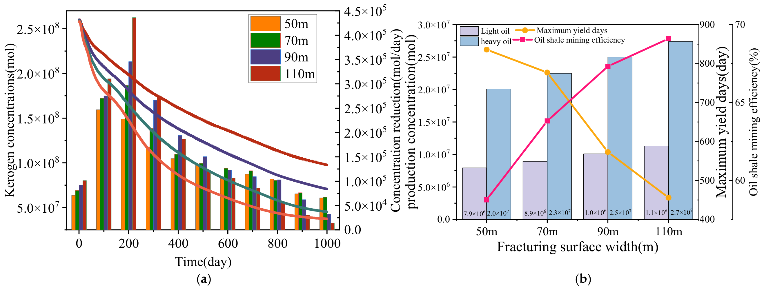
Figure 21a presents the daily kerogen decomposition rate (bar chart) and cumulative kerogen decomposition amount (line chart), which are used to characterize the dynamic evolution of kerogen pyrolysis under different fracture-width conditions. With continuous injection of high-temperature steam, the kerogen pyrolysis reaction in all cases gradually intensifies, and the daily decomposition rate first increases and then decreases, reaching a peak at around 200 days. This indicates that kerogen pyrolysis is rapidly activated as reservoir temperature rises. Subsequently, as the amount of reactive kerogen is continuously depleted, the reaction rate gradually declines, leading to a continuous decrease in the daily decomposition rate. Comparative results under different fracture-width conditions show that a larger fracture width leads to a higher peak decomposition rate and a faster increase in cumulative decomposition. The overall trend follows 110 m > 90 m > 70 m > 50 m. This is mainly because wider fracture planes expand the steam sweep volume, enhance convective heat transfer within the reservoir, and facilitate deeper heat penetration, thereby accelerating kerogen pyrolysis and improving the overall conversion degree. At 1000 days, the 50 m case exhibits the lowest cumulative decomposition amount, indicating the weakest thermal conversion, whereas the 110 m case achieves the highest cumulative decomposition, reflecting the most complete kerogen conversion. In general, increasing the crack width helps to improve the pyrolysis rate and final conversion efficiency of kerogen; however, in practical engineering, it is necessary to comprehensively consider the difficulty of fracturing and the initial production cost to determine the final fracturing surface width.

Figure 21b takes fracture width (50 m, 70 m, 90 m, and 110 m) as the horizontal axis. The bar charts on the left vertical axis represent the molar concentrations of light oil and heavy oil production, respectively. The orange line on the right axis corresponds to the time at which peak oil and gas production occurs, while the pink line further represents the oil shale recovery efficiency. As the fracture width increases from 50 m to 110 m, both light oil and heavy oil production show a continuous increasing trend, with heavy oil exhibiting a more pronounced growth. At a 50 m fracture width, the light oil and heavy oil yields are only 7.9 × 10⁶ mol and 2.0 × 10⁷ mol, respectively, whereas they increase to 1.1 × 10⁷ mol and 2.7 × 10⁷ mol under the 110 m condition. This indicates that widening the fracture channels improves steam seepage and heat transfer conditions, expands the high-temperature pyrolysis zone within the reservoir, promotes more complete kerogen decomposition, and simultaneously enhances both light and heavy hydrocarbon production. The orange curve representing peak production time shows a continuous decreasing trend with increasing fracture width, dropping from approximately 830 days at 50 m to about 450 days at 110 m. This suggests that wider fracture networks accelerate overall reservoir heating, enabling faster kerogen fracturing and significantly advancing the occurrence of peak hydrocarbon production, thereby shortening the overall production cycle. The pink curve representing oil shale recovery efficiency shows a stable increasing trend with fracture width. The 50 m case exhibits the lowest recovery efficiency, while the 110 m case achieves the highest value among all scenarios, confirming that increasing fracture width improves both total hydrocarbon yield and resource conversion efficiency. Among the investigated fracture widths, the 110 m case provides the highest kerogen conversion efficiency, the largest hydrocarbon production, and the earliest production peak.

5.5. Parameter Sensitivity Analysis

To evaluate the relative importance of engineering parameters, a normalized sensitivity coefficient was introduced. The coefficient is defined as [39]:

$$S_i={\displaystyle \frac{(Y_i-Y_{ref})/Y_{ref}}{(X_i-X_{ref})/(X_{\max }-X_{\min })}}$$

(30)

where S_i is the sensitivity coefficient; X_i is the value of the independent variable at the i th point; X_ref is the reference value of the independent variable (Usually, the initial value, the control group value or the value under a standard working condition are taken.); X_max is the maximum value of independent variable; Y_i is the value of the dependent variable at the i th point; Y_ref is the base value of the dependent variable (usually X_ref and Y_ref is the paired data at the same reference point.).

Since reservoir temperature and hydrocarbon production represent different physical processes, different evaluation times were selected. The average reservoir temperature at 600 days was used to evaluate thermal transfer sensitivity because the temperature field approaches quasi-equilibrium at this stage. However, the production sensitivity was evaluated at 400 days because prolonged heating may induce secondary fracturing of liquid hydrocarbons, causing a decline in effective liquid production despite further temperature increase. The specific parameters are shown in

Table 5. Sensitivity analysis table of the influence of engineering parameters on 600-day average reservoir temperature.

Engineering Parameter	Parameter Range	Average Temperature at 600 d (°C)	Relative Temperature Variation (%)	Sensitivity Coefficient (Si)	Sensitivity Ranking
Fracture width (m)	50–110	388.10–526.38	0–35.63	0.36–0.50	2
Fracture number	0–3	170.86–542.38	0–217.59	2.17–3.98	1
Heating well length (m)	16–29	525.06–526.4	0–0.27	0.001–0.003	4
Inter-well angle (°)	0–90	530.7–555.4	0–5.43	0.054–0.117	3

and

Table 6. Sensitivity analysis table of the influence of engineering parameters on the total output of 400 days.

Engineering Parameter	Parameter Range	Cumulative Production at 400 d (mol)	Relative Production Variation (%)	Sensitivity Coefficient (Si)	Sensitivity Ranking
Fracture width (m)	50–110	2.52 × 107–3.85 × 107	0–52.70	0.53–0.55	2
Fracture number	0–3	2.63 × 107–4.70 × 107	0–78.96	0.79–0.93	1
Heating well length (m)	16–29	3.83 × 107–3.86 × 107	0–0.78	0–0.016	4
Inter-well angle (°)	0–90	3.85 × 107–4.88 × 107	0–26.85	0.27–0.59	3

.

The sensitivity analysis indicates that fracture-related parameters dominate the reservoir temperature evolution. Among all investigated parameters, fracture number exhibits the highest sensitivity coefficient (2.17–3.98), indicating that increasing fracture quantity significantly enhances steam migration pathways and heat exchange efficiency. Fracture width shows moderate sensitivity (0.36–0.50), suggesting that fracture expansion improves heat transfer; however, the incremental effect gradually decreases due to enhanced heat dissipation. In contrast, heating well length presents negligible sensitivity, with a sensitivity coefficient below 0.01, indicating that its influence on the reservoir-scale temperature field becomes limited after thermal equilibrium is established.

6. Conclusions

A superheated steam-driven integrated multi-branch well system was proposed for the in-situ conversion of steeply dipping oil shale reservoirs. A coupled thermo–hydro–chemical–mass transport model considering reservoir anisotropy was established to evaluate the heat transfer behavior and optimize key engineering parameters. The main conclusions are as follows:

• Superheated steam preferentially migrates through hydraulic fractures and bedding-parallel high-permeability pathways, resulting in anisotropic heat transfer characteristics. Continuous steam injection gradually develops a connected high-temperature region, and a large proportion of the reservoir exceeds 500 °C after approximately 600 days, providing favorable conditions for large-scale kerogen pyrolysis.
• Compared with the conventional well arrangement, the proposed integrated multi-branch well system improves reservoir heating uniformity and enlarges the effective pyrolysis region under the investigated conditions. The results demonstrate its potential for enhancing heat transfer efficiency in steeply dipping oil shale reservoirs; however, further field-scale validation is required to assess its practical engineering applicability.
• Parametric analysis indicates that the heating well length has a limited influence on reservoir temperature evolution, with 22.5 m providing the highest thermal performance among the investigated cases. Increasing the inter-well angle improves vertical heat transfer and accelerates thermal equilibrium. Increasing fracture number and fracture width enhances steam migration pathways, expands the effective heating region, and promotes kerogen conversion and hydrocarbon production within the simulated scenarios.
• Sensitivity analysis shows that fracture-related parameters have a stronger influence on reservoir thermal performance than heating well length and inter-well angle. The investigated parameter combinations provide improved thermal and production performance based on numerical simulations; however, the final engineering design should consider fracture construction feasibility, energy consumption, heat losses, and techno-economic factors. Further experimental and field studies are needed to validate the long-term performance of the proposed system.

7. Future Outlook

Although this study provides insights into heat transfer analysis of multi-branch well systems in steeply dipping oil shale reservoirs, several limitations remain. First, although anisotropic thermal and hydraulic properties are considered, the geological heterogeneity of actual reservoirs, including spatial variations in mineral composition, organic matter distribution, permeability, and natural fracture networks, is simplified. Second, hydraulic fractures are represented as equivalent high-permeability zones with fixed geometrical parameters, while dynamic fracture propagation and permeability evolution during thermal stimulation are not considered. Third, the chemical reaction model mainly focuses on kerogen conversion and liquid hydrocarbon generation, whereas detailed gas-phase reactions, hydrogen production, and secondary fracturing mechanisms require further investigation. In addition, the current model assumes a constant steam injection condition and does not fully consider wellbore-scale heat loss and pressure variation. Moreover, due to the limited availability of field-scale data, further experimental and field validations are required.

Future studies should incorporate geological stochastic modeling, coupled thermo-hydro-mechanical fracture evolution, comprehensive reaction networks, and wellbore-reservoir coupling to improve prediction accuracy. Furthermore, techno-economic analysis and environmental assessment should be integrated to evaluate the practical feasibility of the proposed system under different geological conditions.

References

1. Fan, C.; Guo, W.; Li, Q.; Wang, Y.; Li, Y.; Liu, Z. A physicochemical model for accurate prediction of oil shale in-situ conversion. Chem. Eng. J. 2026, 530, 173545. [Google Scholar] [CrossRef]
2. Wang, L.; Wang, Z.; Zhao, Y.; Zhang, R.; Yang, D.; Kang, Z.; Zhao, J. Macroscopic seepage and microstructural behavior of oil shale using water vapor injection during mining. J. Rock Mech. Geotech. Eng. 2025, 17, 1489–1509. [Google Scholar] [CrossRef]
3. Pan, Y.; Zheng, L.; Liu, Y.; Wang, Y.; Yang, S. A review of the current status of research on convection-heated in situ extraction of unconventional oil and gas resources (oil shale). J. Anal. Appl. Pyrolysis 2023, 175, 106200. [Google Scholar] [CrossRef]
4. Sun, D.; Huang, X.; Yang, D.; Wang, L.; Kang, Z. Multifractal-theory-based investigation of the high-temperature steam-driven multiscale evolution mechanisms of the pore-fracture system in oil shale. Appl. Therm. Eng. 2026, 292, 130353. [Google Scholar] [CrossRef]
5. Shen, Y.; Zhao, Y.; Song, Y.; Shan, X.; Yao, Y.; Bian, Y.; Jiang, N.; Wang, S.; He, W. Carbon-isotope and pyrolysis-product evolution during pyrolysis of Fushun oil shale: Implications for in-situ pyrolysis project. J. Anal. Appl. Pyrolysis 2026, 196, 107784. [Google Scholar] [CrossRef]
6. Huang, X.; Yang, D.; Zhao, J. Spatiotemporal evolution of temperature fields and fracture evolution in oil shale under superheated steam heating. Int. J. Therm. Sci. 2026, 220, 110430. [Google Scholar] [CrossRef]
7. Kang, Z.; Xie, H.; Zhao, Y.; Zhao, J. The feasibility of in-situ steam injection technology for oil shale underground retorting. Oil Shale 2020, 37, 119–138. [Google Scholar] [CrossRef]
8. Song, X.; Zhang, C.; Shi, Y.; Li, G. Production performance of oil shale in-situ conversion with multilateral wells. Energy 2019, 189, 116145. [Google Scholar] [CrossRef]
9. Song, S.; Mei, S.; Hu, Y.; Li, Q.; Chen, Z.; Zhang, S. Research on the thermo-hydro-mechanical coupling simulation and deformation spatiotemporal evolution for the entire process of oil shale in-situ mining. Eng. Geol. 2024, 339, 107643. [Google Scholar] [CrossRef]
10. Wang, L.; Gao, C.; Xiong, R.; Zhang, X.; Guo, J. Development review and the prospect of oil shale in-situ catalysis conversion technology. Pet. Sci. 2024, 21, 1385–1395. [Google Scholar] [CrossRef]
11. Lei, Z.; Zhang, Y.; Yang, Z.; Shi, Y.; Zhang, H.; Li, X.; Cui, Q. Numerical simulation of oil shale in-situ exploration productivity comparison between steam injection and electrical heating. Appl. Therm. Eng. 2024, 238, 121928. [Google Scholar] [CrossRef]
12. Zhang, Z.; Bricen, M.; Li, S.; Xu, T.; Li, Y.; Xie, Z.; Li, X. Evaluating heating strategies for efficient in-situ shale oil conversion: A numerical approach using THC coupled modeling. Appl. Therm. Eng. 2025, 270, 126203. [Google Scholar] [CrossRef]
13. Zhu, J.; Yi, L.; Yang, Z.; Li, X. Numerical simulation on the in situ upgrading of oil shale reservoir under microwave heating. Fuel 2021, 287, 368–381. [Google Scholar] [CrossRef]
14. Cheng, K.; Zhang, Y.; Chen, Y.; Guo, L. Experimental study on the generation of oil and gas from oil shale in sub/supercritical water environment. Fuel 2026, 411, 138054. [Google Scholar] [CrossRef]
15. Zhang, Y.; Wang, L.; Zhao, J.; Zhang, R. Fracture morphology-convective heating coupled effects on the in-situ pyrolysis behavior of oil shale under stress constraint. J. Anal. Appl. Pyrolysis 2026, 196, 107780. [Google Scholar] [CrossRef]
16. Wang, G.; Liu, S.; Yang, D.; Fu, M. Numerical study on the in-situ pyrolysis process of steeply dipping oil shale deposits by injecting superheated water steam: A case study on Jimsar oil shale in Xinjiang, China. Energy 2022, 239, 122182. [Google Scholar] [CrossRef]
17. Wang, L.; Zhang, Y.; Zou, R.; Yuan, Y.; Zou, R.; Huang, L.; Liu, Y.; Ding, J.; Meng, Z. Applications of molecular dynamics simulation in studying shale oil reservoirs at the nanoscale: Advances, challenges and perspectives. Pet. Sci. 2025, 22, 234–254. [Google Scholar] [CrossRef]
18. Guo, W.; Pan, J.; Yang, Q.; Li, Q.; Deng, S.; Zhu, C. Study of the residual carbon oxidation trigger mechanism in fractured oil shale formation under real condition. Int. Commun. Heat Mass Transf. 2025, 160, 108369. [Google Scholar] [CrossRef]
19. Wang, Z.; Wang, T.; Yan, X. Investigation of the current state of catalytic pyrolysis technology for oil shale: A review. J. Anal. Appl. Pyrolysis 2025, 192, 137238. [Google Scholar] [CrossRef]
20. Wang, G.; Yin, Q.; Jia, H.; Feng, G.; Ma, H.; Wang, L.; Klitzsch, N.; Yan, C.; Liu, S.; Hu, Z.; et al. Experimental study on real-time seepage-heat transfer characteristics of fractured granite during the cyclic liquid nitrogen injecting the hot dry rock reservoir. Case Stud. Therm. Eng. 2025, 76, 107424. [Google Scholar] [CrossRef]
21. Jia, B.; Wang, S.; Yang, J.; Huang, Z. Multi-stage kinetic analysis and product distribution prediction for oil shale pyrolysis. Fuel 2026, 420, 138994. [Google Scholar] [CrossRef]
22. Yuan, S.; Li, L.; Jiang, H.; Shen, Z.; He, H.; Du, K.; Wang, J.; Ren, Z.; Hu, H.; Li, L. In-situ catalytic pyrolysis of oil shale: Recent advances and perspectives. J. Anal. Appl. Pyrolysis 2026, 197, 107798. [Google Scholar] [CrossRef]
23. Jin, J.; Deng, Y.; Sun, J.; Lv, K.; Ren, K.; Song, C. Enhanced in-situ pyrolysis of oil shale by supercritical CO2 coupled with nanocatalysts: Mechanisms and product evolution. J. Anal. Appl. Pyrolysis 2026, 197, 107833. [Google Scholar] [CrossRef]
24. Yang, S.; Wang, H.; Zheng, J.; Pan, Y.; Ji, C. Comprehensive review: Study on heating rate characteristics and coupling simulation of oil shale pyrolysis. J. Anal. Appl. Pyrolysis 2024, 177, 106289. [Google Scholar] [CrossRef]
25. Song, Y.; Song, Z.; Mo, Y.; Zhou, Q.; Jing, Y.; Chen, F.; Tian, S.; Chen, Z. Determination of minimum miscibility and near-miscibility pressures for CO2-oil mixtures in shale reservoirs. Fuel 2025, 388, 134531. [Google Scholar] [CrossRef]
26. Li, Q.; You, D.; Li, Q.; Wang, F.; Wang, Y.; Yang, Y. Analysis of Sedimentation Behavior and Influencing Factors of Solid Particles in CO2 Fracturing Fluid. Processes 2025, 13, 4049. [Google Scholar] [CrossRef]
27. Ao, F.; Li, Q.; Qiang, L.; Wu, J.; Wang, F.; Yan, C. Numerical Simulation Investigation of Fracture Propagation Behavior Patterns and Sensitivity Factors of Oil Shale Reservoirs in the Xunyi Region Considering the Influence of Natural Fracture. Geofluids 2025, 2025, 2762142. [Google Scholar] [CrossRef]
28. Deori, P.; Ahmad, A.; Routray, A. Hybrid quasi Z source multi output converter system with performance control and real time validation for photovoltaic microgrid. Sci. Rep. 2026, 16, 6255. [Google Scholar] [CrossRef] [PubMed]
29. Ma, H.; Wang, G.; Feng, G.; Jia, H.; Wang, L.; Zhou, F.; Liu, S.; Heng, S.; Wang, W. Experimental study on the mechanical properties of granite after circulating liquid nitrogen subjected to real time high temperature. Geoenergy Sci. Eng. 2025, 246, 213624. [Google Scholar] [CrossRef]
30. Wang, G.; Yin, Q.; Jia, H.; Feng, G.; Liu, S.; Heng, S. Experimental Study on Anisotropic Pore-Fracture and Real-Time Permeability Evolution of Fractured Oil Shale Under High Temperature and Triaxial Stress: A Case Study of Jimsar Oil Shale in Xinjiang, China. Rock Mech. Rock Eng. 2026, 59, 183–205. [Google Scholar]
31. Zhu, J.; Li, F.; Wang, H.; Yang, Z.; Chen, H.; Zhu, H. Numerical analysis of microwave-enhanced oil shale pyrolysis by rotation turntable based on the Arbitrary Lagrangian-Eulerian method. Fuel 2024, 371, 131925. [Google Scholar] [CrossRef]
32. Niu, X.; Lyu, C.; Feng, S.; Zhou, Q.; Xin, H.; Xiao, Y.; Li, C.; Dan, W. Lamina combination characteristics and differential shale oil enrichment mechanisms of continental organic-rich shale: A case study of Triassic Yanchang Formation Chang 73 sub-member, Ordos Basin, NW China. Pet. Explor. Dev. 2025, 52, 316–329. [Google Scholar] [CrossRef]
33. Wang, G.; Zhou, F.; Jia, H.; Wang, L.; Klitzsch, N.; Feng, G.; Yan, C.; Ma, H.; Liu, S.; Yin, Q.; et al. Heat extraction performance of multi-level, multi-branch, closed loop coaxial horizontal borehole heat exchanger geothermal system. Appl. Therm. Eng. 2025, 269, 126045. [Google Scholar] [CrossRef]
34. Zheng, S.; Liu, B.; Erfan, M.; Liu, Y.; Tian, S. Sustainable in-situ steam injection approach for shale oil extraction in Xinjiang, China: A technical and economic analysis. Energy 2024, 308, 132986. [Google Scholar] [CrossRef]
35. Jervell, V.; Wilhelmsen, O. Revised Enskog theory for Mie fluids: Prediction of diffusion coefficients, thermal diffusion coefficients, viscosities, and thermal conductivities. J. Chem. Phys. 2023, 158, 224101. [Google Scholar] [CrossRef] [PubMed]
36. Lee, K.; Moridis, G.; Ehlig-Economides, C. Numerical simulation of diverse thermal in situ upgrading processes for the hydrocarbon production from kerogen in oil shale reservoirs. Energy Explor. Exploit. 2017, 35, 315–337. [Google Scholar] [CrossRef]
37. Kuang, L.; Wu, S.; Xing, H.; Wu, K.; Shen, Y.; Wang, Z. Key parameters and evaluation methods for large-scale production of lacustrine shale oil. Pet. Explor. Dev. 2025, 52, 883–893. [Google Scholar] [CrossRef]
38. Lauwerier, H. The transport of heat in an oil layer caused by the injection of hot fluid. Appl. Sci. Res. 1955, 5, 145–150. [Google Scholar] [CrossRef]
39. Wieckowski, J.; Salabun, W. Sensitivity analysis approaches in multi-criteria decision analysis: A systematic review. Appl. Soft Comput. 2023, 148, 110915. [Google Scholar] [CrossRef]
Figure 1. Schematic diagram of in-situ development engineering in a steeply inclined oil shale reservoir.
Energies 19 03473 g001
Figure 2. Schematic diagram of multi-branch well system structure.
Energies 19 03473 g002
Figure 3. (a) Location of the Jimsar mining area; (b) geological profile at the north foot of the Bogda mountain, and (c) profile of the Jimsar oil shale deposit. Adapted from [16].
Energies 19 03473 g003
Figure 4. Geometric model. (a) vertical, (b) parallel.
Energies 19 03473 g004
Figure 5. Numerical simulation grid division and lateral line distribution of the survey surface. (a) Numerical simulation grid division, (b) simulated the side line, side position distribution.
Energies 19 03473 g005
Figure 6. 600-day average temperature and calculation time under different grid numbers.
Energies 19 03473 g006
Figure 7. Single fracture heat transfer model.
Energies 19 03473 g007
Figure 8. Comparison between analytical and simulated solutions. (a) represents the temperature variation law of different measuring points, (b) represents the temperature distribution at different times.
Energies 19 03473 g008
Figure 9. (Row 1): thermal fluid pressure; (row 2): velocity streamline; (row 3): Isothermal surface.
Energies 19 03473 g009
Figure 10. The temperature and pore pressure distribution of ab, cd lateral line. (a) The temperature distribution law of a sideline ab, (b) The temperature distribution law of a sideline cd, (c) The pressure distribution law of c sideline ab, (d) The pressure distribution law of c sideline cb.
Energies 19 03473 g010
Figure 11. Comparison of temperature field between two schemes.
Energies 19 03473 g011
Figure 12. Cost comparison of two schemes.
Energies 19 03473 g012
Figure 13. Temperature variation law of side a. (a) represents the temperature cloud diagram corresponding to the heating well length of 16 m, (b) represents the temperature cloud diagram corresponding to the heating well length of 22.5 m, (c) represents the temperature cloud diagram corresponding to the heating well length of 19 m.
Energies 19 03473 g013
Figure 14. Comparison of temperature and production of different heating well lengths. (a) Temperature, (b) yield.
Energies 19 03473 g014
Figure 15. Temperature changes of different injection well angles. (a) A represents the temperature cloud diagram corresponding to the heating well angle of 0°, (b) A represents the temperature cloud diagram corresponding to the heating well angle of 30°, (c) A represents the temperature cloud diagram corresponding to the heating well angle of 60°, (d) A represents the temperature cloud diagram corresponding to the heating well angle of 30°.
Energies 19 03473 g015
Figure 16. Comparison of angle temperature and production of different heating wells. (a) Temperature, (b) yield.
Energies 19 03473 g016
Figure 17. The number of different fracturing surfaces is greater than the proportion of 500 °C is surfaces and regions. (a) Equivalence surface, (b) Proportion of regions above 500 °C.
Energies 19 03473 g017
Figure 18. Comparison of cumulative consumption and product of kerogen under different numbers of fracturing surfaces. (a) Comparison of cumulative consumption of kerogen, (b) Product comparison.
Energies 19 03473 g018
Figure 19. Side b shows the variation of temperature distribution with time for different widths of fracture surface. (a) represents the temperature cloud diagram corresponding to the width of the fracturing surface of 50 m, (b) represents the temperature cloud diagram corresponding to the width of the fracturing surface of 70 m, (c) represents the temperature cloud diagram corresponding to the width of the fracturing surface of 90 m, (d) A represents the temperature cloud diagram corresponding to the width of the fracturing surface of 110 m.
Energies 19 03473 g019
Figure 20. Comparison of ab temperature distribution and reservoir temperature at different fracturing surface widths. (a) Sideline ab temperature distribution, (b) Comparison of average reservoir temperature.
Energies 19 03473 g020
Figure 21. Comparison of cumulative consumption and product of kerogen under different fracturing surface widths. (a) Cumulative kerogen consumption, (b) yield comparison.
Energies 19 03473 g021