Online SOH Estimation of Lithium-Ion Batteries with a Sequential Gaussian Process

Abstract

Lithium-ion batteries (LIBs) have been widely used in different fields as energy storage systems, such as electric vehicles and power grids. The performance of LIBs degrades with usage, which poses challenges for battery management. Thus, accurate online estimation of the state of health (SOH) is critical to ensure reliability and prolong the service time of LIBs. To achieve this, data-driven methods have become popular due to the capability of learning the mapping between SOH and measurements without prior knowledge of aging mechanisms. However, the online estimation performance of these methods cannot be guaranteed, since the models are trained offline and do not have the capability of online updating when new data are collected. In addition, the inputs for these methods are constructed with the voltage–capacity (V-Q) curve within a fixed voltage interval, which can hardly be realized in real-life applications due to the randomness of the charging or discharging process. This study proposes a Sequential Gaussian Process (Seq-GP) model-based LIB SOH estimation method, where model parameters can be updated using newly collected LIB data, such that online estimation can be fulfilled. Moreover, a novel feature extraction method is presented using random parts of the LIB V-Q curve to meet the requirements for practical applications. The proposed method is evaluated on two public battery datasets, showing competitive estimation accuracy together with online updating, uncertainty quantification, and low computational cost under the tested protocol. The results will be beneficial for online SOH estimation of LIBs in practical scenarios.

1. Introduction

With the increasing concern of carbon emissions from fossil energy, renewable and clean energy has become a hot research topic [1,2]. Li-ion batteries (LIBs) are widely used in electric vehicles (EVs) and consumer electronics as energy storage systems with the advantages of high energy and power density, as well as a wide operating temperature range [3,4]. However, one of the technical difficulties that affects the management of LIBs is to accurately evaluate the state of health (SOH). The SOH of a LIB is typically determined by the ratio of some performance parameters, such as capacity and internal resistance, and current values to their initial values after a period of operation [5]. SOH serves as an indicator of the degradation level of LIBs, which provides information about battery health. Therefore, an accurate SOH estimation is essential for the reliable and effective operation of LIBs.

During the last few decades, extensive research efforts have been dedicated to estimating the SOH of LIBs. These methods can be roughly categorized into two types, namely model-based and data-driven methods [6,7]. Within the model-based methods, physical or empirical governing equations are firstly employed to describe the operation of LIBs, and then different filtering algorithms are utilized, such as the Kalman filter [8,9] and particle filter [10,11], to update model parameters for SOH estimation. For example, electrochemical model (EM) [10]-based methods simulate the internal electrochemistry of LIBs using first-principles equations and can provide accurate estimation results. However, the involved partial differential equations require a huge computational cost, limiting their applications in online systems. Different from the EM, the equivalent circuit model (ECM) [8] has been developed by describing the phenomenological behavior of LIBs with simple circuit models. Although the ECM can be utilized for real-time estimation of SOH, the simplification of internal chemical reactions results in unreliable estimation under various operating conditions [12].

In addition to the model-based methods, data-driven approaches have become popular in the SOH estimation field. These methods directly learn the intrinsic relationship from collected data without expert knowledge [13]. For instance, Naha et al. [14] collected the derived voltage values and the average temperature during charging to construct the feature vector of a neural network for SOH estimation; Meng et al. [15] designed a novel SVM structure and extracted features from a voltage curve to get SOH estimation; Guo et al. [16] proposed an adaptive regressive vector machine based on particle swarm optimization to ensure SOH estimation. However, only point estimations are provided with these methods, and the estimation uncertainty cannot be generated for better decision-making.

To alleviate this drawback, Gaussian Process (GP)-based models have received considerable attention. These models can directly provide the mean estimation of SOH as well as the uncertainty associated with the estimation, which could be valuable for users to make an informed decision [17]. Moreover, the nonparametric nature and simple implementation without compromising performance enable GP to be more flexible than other state-of-the-art methods. The key to realizing accurate SOH estimation with GP is to construct suitable inputs based on measured signals for model training. Li et al. [18] took health factors extracted from the incremental capacity (IC) curves as inputs for GP to estimate battery SOH. In [19], four specific parameters extracted from charging curves were used to develop a novel GP model for SOH estimation. Richardson et al. [20] employed GP to construct a data-driven in situ capacity estimation method by using a segment from the charging voltage curve. The successful implementation of these methods requires the voltage–capacity (V-Q) curves within a specific voltage interval for input construction. However, in real-world applications, the charging or discharging process of LIBs generally starts and ends at random SOC levels; i.e., only random parts of V-Q curves can be obtained, which greatly limits the applicability of these methods. Therefore, it is critical to develop a model that can achieve SOH estimation with random partial data.

There are some methods that have been developed to estimate SOH with random parts of V-Q curves. For example, Feng et al. [21] trained an SVM model with complete charging curves and stored the corresponding support vectors (SVs). During online estimation, a random segment of the charging curve was compared to the stored SVs to determine SOH. However, the random segments are required to be within the voltage interval where the IC curve is monotonic, which greatly affects the applicability of this method. In [22], statistical features, i.e., mean and standard deviation, from the capacity increment sequence were extracted as the input for GP to estimate SOH. Although the problem of random partial V-Q curves is alleviated to some extent, these models cannot be updated online after the training process is completed. In real-life applications, data is usually collected in a sequential manner; that is, more data will be obtained as time passes. The newly collected data can provide additional information to improve SOH estimation. One simple solution is to retrain the whole model with both historical and new data. However, it is computationally expensive and thus inappropriate for online applications. Therefore, it is beneficial to develop a model that can incorporate the information from new data for model updates rather than retraining.

To the best of our knowledge, online updating under random partial V-Q curves remains an open challenge in existing methods. To address this gap, the primary goal of this paper is to establish an accurate, computationally efficient, and partial-curve-robust online SOH estimation framework that can handle random partial V-Q curves and sequentially collected data. To achieve this goal, the following three specific tasks are formulated and tackled in this study: (1) a Sequential Gaussian Process (Seq-GP) updating framework is adapted for online SOH estimation with an efficient parameter update mechanism to overcome the computational burden and lack of online updating capability of standard GP models; (2) a robust feature extraction method must be created to construct informative inputs from arbitrary random segments of the V-Q curves; and (3) the effectiveness and cross-dataset applicability of the proposed framework are systematically evaluated using two public battery datasets with different aging protocols. Accordingly, in this paper, we propose a sequential GP model for battery SOH estimation, which can realize online updates of model parameters with random partial V-Q curves. Specifically, the variational sparse approximation technique [23] is introduced to realize online updates of the GP with newly collected data.

Under this framework, a variational lower bound is derived for the marginal likelihood of new data given the historical data, based on which an analytical updating algorithm is realized. In addition, to deal with the problem that only random parts of V-Q curves can be obtained, a new input feature is established with the partial capacity sequence for model training. The main contributions of this paper are summarized as follows:

(1)

A Seq-GP model is proposed to estimate LIB SOH, where the information from newly collected data can be utilized to update model parameters, thus fulfilling online estimation.

(2)

A novel feature from random parts of LIB V-Q curves is constructed to accommodate practical applications where the full curve cannot be obtained.

(3)

The effectiveness and partial-curve robustness of the proposed method are demonstrated on two public LIB datasets under different aging protocols.

The rest of the paper is organized as follows. In Section 2, the details of the proposed model and feature construction method are introduced. Battery datasets used to validate the performance of the proposed method are presented in Section 3. Section 4 provides the estimation results and comparisons with some existing methods. Conclusions of this paper are given in Section 5.

2. Methodology

In this study, GP is used to model the relationship between input features and battery SOH. As a Bayesian nonparametric modeling method, GP has been widely applied in many fields due to its flexibility and probabilistic nature [24]. However, the computational complexity of regular GP becomes unaffordable as the amount of data increases, which limits its applicability in real-world scenarios. Thus, an online learning method based on variational sparse approximation is proposed in this section, which not only alleviates the computational burden of regular GP but can also extract information from sequentially collected data for model updates. In addition, the charging or discharging process of LIBs is random, which complicates the input construction for the GP model. In this section, a novel feature from the partial V-Q curve is built to realize accurate SOH estimation.

2.1. Regular Gaussian Process

To facilitate the illustration of our proposed method, regular GP is introduced first in this subsection. We assume the $i^{th}$ input is ${\mathit{x}}_i\in {\mathcal{R}}^m$ and the corresponding output, i.e., battery SOH in this paper, is $y\left({\mathit{x}}_i\right)$. With these notations and under the context of GP, we have

$$y\left({\mathit{x}}_i\right)=f\left({\mathit{x}}_i\right)+ϵ\left({\mathit{x}}_i\right),$$

(1)

$$f\left({\mathit{x}}_i\right)~\mathcal{G}\mathcal{P}\left(m\left({\mathit{x}}_i\right),k({\mathit{x}}_i,{\mathit{x}}_j)\right),$$

(2)

where $ϵ\left({\mathit{x}}_i\right)$ is the observation noise with independent, identically distributed normal distribution, i.e., $ϵ\left({\mathit{x}}_i\right)~\mathcal{N}\left(0,{\sigma }^2\right)$; $m\left({\mathit{x}}_i\right)$ is the mean and usually assumed to be zero for simplicity; $k({\mathit{x}}_i,{\mathit{x}}_j)$ represents the covariance function and quantifies the correlation between the $i^{th}$ and $j^{th}$ observations. Among various covariance functions, the squared exponential (SE) covariance function is one of the most widely used, whose expression is as follows:

$$k\left({\mathit{x}}_i,{\mathit{x}}_j\right)={\lambda }^2\exp \left(-{\displaystyle \frac{{\left({\mathit{x}}_i-{\mathit{x}}_j\right)}^T\left({\mathit{x}}_i-{\mathit{x}}_j\right)}{2l^2}}\right),$$

(3)

where $\lambda$ and $l$ are hyperparameters. We also adopted this covariance function in the current study. The SE covariance function captures the highly nonlinear degradation dynamics of LIBs. Electrochemical aging mechanisms—SEI growth, active material loss, and lithium plating—exhibit complex nonlinear interactions with external measurements, which the SE kernel flexibly models without requiring explicit prior knowledge of the underlying governing equations.

Suppose there are $n$ input–output pairs in the training set, and the inputs, outputs, and latent function values are denoted as $\mathit{X}={\left[{\mathit{x}}_1,\dots ,{\mathit{x}}_n\right]}^T$, $\mathit{y}={\left[y\left({\mathit{x}}_1\right),\dots ,y\left({\mathit{x}}_n\right)\right]}^T$ and $\mathit{f}={\left[f\left({\mathit{x}}_1\right),\dots ,f\left({\mathit{x}}_n\right)\right]}^T$, respectively. Using the property of GP (that is, any finite collection of random variables follows a normal distribution [24]), we have

$$\mathit{y}~\mathcal{N}\left(0,k\left(\mathbf{X},\mathbf{X}\right)+{\sigma }^2{\mathbf{I}}_n\right),$$

(4)

where $k\left(\mathbf{X},\mathbf{X}\right)$ is the covariance matrix of $\mathit{f}$, whose entry in the $i^{th}$ row and $j^{th}$ column is $k({\mathit{x}}_i,{\mathit{x}}_j)$, and ${\mathbf{I}}_n$ is an $n\times n$ identity matrix. Thus, the log-likelihood function of the model can be obtained as follows:

$$\log p\left(\mathit{y}\right)=\log \left[\mathcal{N}\left(\mathit{y}\right|0,\mathsf{\Lambda })\right]=-{\displaystyle \frac{nlog2\pi }{2}}-{\displaystyle \frac{{\mathit{y}}^{\mathit{T}}{\mathsf{\Lambda }}^{-1}\mathit{y}}{2}}-{\displaystyle \frac{\log \left|\mathsf{\Lambda }\right|}{2}},$$

(5)

where ${\mathsf{\Lambda }=k\left(\mathbf{X},\mathbf{X}\right)+\sigma }_n^2{\mathbf{I}}_n$ Based on this, the model parameters $\mathit{\theta }=\left\{\lambda ,l,{\sigma }^2\right\}$ can be optimized through the maximization of (5). Then, for a given new input ${\mathit{x}}_{*}$, inference for the corresponding output $y_{\mathit{*}}$ is

$$p\left(y_{\mathbf{*}}\right|\mathit{y},\mathbf{X},{\mathit{x}}_{\mathrm{*}})=N({\mu }_{\mathrm{*}},{\sigma }_{\mathrm{*}}^2),$$

(6)

where

$${\mu }_{*}=k\left({\mathit{x}}_{*},\mathbf{X}\right){\mathsf{\Lambda }}^{-1}\mathit{y},$$

(7)

$${\sigma }_{\mathrm{*}}^2=k\left({\mathit{x}}_{\mathrm{*}},{\mathit{x}}_{\mathrm{*}}\right)-k\left({\mathit{x}}_{\mathrm{*}},\mathbf{X}\right){\mathsf{\Lambda }}^{-1}k\left(\mathbf{X},{\mathit{x}}_{\mathrm{*}}\right)+{\sigma }^2,$$

(8)

According to (6), the estimation of $y_{\mathit{*}}$ can be given by the mean value ${\mu }_{*}$ and the estimation uncertainty can be measured by the variance ${\sigma }_{*}^2$. Generally, a 95% confidence interval for the estimation can be obtained as follows:

$$[{\mu }_{\mathrm{*}}-1.96{\sigma }_{\mathrm{*}},{\mu }_{\mathrm{*}}+1.96{\sigma }_{\mathrm{*}}],$$

(9)

Although regular GP is a flexible Bayesian nonparametric method, its complexity is $O\left(n^3\right)$ for training and $O\left(n^2\right)$ for testing [23]. To overcome these limitations, the next section introduces a sequential GP formulation based on variational sparse approximation, which not only reduces the computational complexity to $O\left(M^3\right)$(with $M$ ≪ n being the number of inducing points) but also enables online parameter updates as new partial V–Q curves become available. Thus, when the amount of training samples is huge, the computational complexity would be unaffordable. In addition, in real-world applications, the data are usually collected in a sequential manner; i.e., more data will be collected as time passes. As a result, if we directly combine new data with historical data and retrain the whole model, the computational effort will become increasingly intensive. Therefore, it is critical to develop a GP model that can effectively incorporate newly collected data for model updates.

2.2. Sequential Gaussian Process Based on Variational Sparse Approximation

An online learning framework based on GP is developed in this section, which can alleviate the computational burden of regular GP and, at the same time, incorporate sequential observations. To represent the data obtained in a sequential manner, subscripts are introduced into the notation system. Specifically, let ${\mathcal{D}}_t=\{{\mathit{X}}_t,{\mathit{y}}_t\}$ denote the data collected at time $t$, i.e., $t^{th}$ data batch, and ${\mathit{X}}_t={\left[{\mathit{x}}_{t,1},\dots ,{\mathit{x}}_{t,n_t}\right]}^T$ and ${\mathit{y}}_t={\left[y_{t,1},\dots ,y_{t,n_t}\right]}^T$ denote the inputs and outputs, respectively. Let the latent function values evaluated at the inputs ${\mathbf{X}}_t$ be ${\mathit{f}}_t=f\left({\mathbf{X}}_t\right)={\left[f\left({\mathit{x}}_{t,1}\right),\dots ,f\left({\mathit{x}}_{t,n_t}\right)\right]}^T$. In addition, let ${\mathcal{D}}_{1:t}$, ${\mathbf{X}}_{1:t}$, ${\mathit{y}}_{1:t}$, ${\mathit{f}}_{1:t}$ be the corresponding components of the first $t$ batches ($t\ge 1$).

The sequential update adopted in this study builds on the sparse online and streaming sparse Gaussian Process literature [25,26]. Following this line of work, the inducing-variable posterior is used as a compact representation of historical observations, enabling newly collected data to be incorporated without full retraining. In this paper, this update mechanism is specialized to online battery SOH estimation with random partial V-Q observations. Specifically, the sequential sparse-GP formulation is coupled with the PCA-based feature constructed from partial V-Q segments, so that the model can update its posterior distribution and predictive uncertainty as new battery data become available. This integration provides an online SOH estimation framework that combines partial-curve feature extraction, sequential Bayesian updating, and uncertainty quantification.

The key to reducing computational complexity and realizing online updating is to introduce a number of inducing points, which serve as a bridge between new observations and target prediction. Specifically, we assume the information from data can be summarized with these inducing points; i.e., ${\mathcal{D}}_{\mathcal{U}}=\{{\mathbf{X}}_{\mathcal{U}},{\mathit{f}}_{\mathcal{U}}\}$ with ${\mathbf{X}}_{\mathcal{U}}={\left[{\mathit{x}}_{\mathcal{U},1},\dots ,{\mathit{x}}_{\mathcal{U},n_{\mathcal{U}}}\right]}^T$ and ${\mathit{f}}_{\mathcal{U}}=f\left({\mathbf{X}}_{\mathcal{U}}\right)$. This can be mathematically represented as follows:

$$p(f_{\mathrm{*}},{\mathit{f}}_{\mathcal{U}}|{\mathit{y}}_{1:t})=p(f_{\mathrm{*}}\left|{\mathit{f}}_{\mathcal{U}}\right)p\left({\mathit{f}}_{\mathcal{U}}\right|{\mathit{y}}_{1:t}),$$

(10)

where $f_{*}=f\left({\mathit{x}}_{*}\right)$ is the latent function value evaluated at any arbitrary input ${\mathit{x}}_{*}$. With this assumption, now the objective of online learning is to sequentially update $p\left({\mathit{f}}_{\mathcal{U}}\right|{\mathit{y}}_{1:t})$ with $p\left({\mathit{f}}_{\mathcal{U}}\right|{\mathit{y}}_{1:t-1})$ and ${\mathit{y}}_t$. However, since the posterior density $p\left({\mathit{f}}_{\mathcal{U}}\right|{\mathit{y}}_{1:t})$ usually does not have a closed-form expression, a variational sparse approximation method is adopted in this study. That is, variational density is introduced to approximate the true posterior, i.e., ${\phi }_t\left({\mathit{f}}_{\mathcal{U}}\right)\approx p\left({\mathit{f}}_{\mathcal{U}}\right|{\mathit{y}}_{1:t})$. With these notations, the following update is restated/adapted for the notation used in this study to realize the online update of ${\phi }_t\left({\mathit{f}}_{\mathcal{U}}\right)$.

Lemma 1.

Suppose ${\phi }_t\left({\mathit{f}}_{\mathcal{U}}\right)\approx p\left({\mathit{f}}_{\mathcal{U}}\right|{\mathit{y}}_{1:t})=MVN({\mathit{\alpha }}_t,{\mathit{\Sigma }}_t)$ is the variational approximation of the posterior density of ${\mathit{f}}_{\mathcal{U}}$ conditional on the first $t$ batches of data. If the assumption of (10) is satisfied, then the mean and covariance of ${\phi }_t\left({\mathit{f}}_{\mathcal{U}}\right)$ are as follows:

$${\mathit{\alpha }}_t={\mathit{\Sigma }}_t\left({\mathit{\Sigma }}_{t-1}^{-1}{\mathit{\alpha }}_{t-1}+{\sigma }_t^{-2}{\mathit{G}}_t^T{\mathit{y}}_t\right),$$

(11)

$${\mathit{\Sigma }}_t={\left({\sigma }_t^{-2}{\mathit{G}}_t^T{\mathit{G}}_t+{\mathit{\Sigma }}_{t-1}^{-1}\right)}^{-1},$$

(12)

where ${\mathit{\alpha }}_{t-1}$ and ${\mathit{\Sigma }}_{t-1}$ are respectively the mean and covariance of ${\mathit{f}}_{\mathcal{U}}$ updated with the first $t-1$ data batches, ${\mathit{G}}_t={\mathit{K}}_{t\mathcal{U}}{\mathit{K}}_{\mathcal{U}\mathcal{U}}^{-1}$ , and ${\mathit{K}}_{\mathcal{i}\mathcal{j}}=k\left({\mathit{X}}_{\mathcal{i}},{\mathit{X}}_{\mathcal{j}}\right),\left(\mathcal{i},\mathcal{j}\in \{t,\mathcal{U}\}\right)$ is the covariance matrix constructed with the corresponding inputs ${\mathit{X}}_{\mathcal{i}}$ and ${\mathit{X}}_{\mathcal{j}}$ . In addition, the unknown parameters in (11) and (12) can be obtained through the maximization of the following lower bound:

$$\mathcal{J}\left({\mathit{\theta }}_t\right)=\log \mathcal{N}\left({\mathit{y}}_t\right|{\mathbf{G}}_t{\mathit{\alpha }}_{t-1},{\mathbf{G}}_t{\mathsf{\Sigma }}_{t-1}{\mathbf{G}}_t^T+{\sigma }_t^2{\mathbf{I}}_{n_t})-C,$$

(13)

where ${\mathit{\theta }}_t=\left\{{\lambda }_t,l_t,{\sigma }_t^2\right\}$ incorporates all the parameters to be optimized, $C=-{\displaystyle \frac{{\sigma }_t^{-2}}{2}}tr\left({\mathit{K}}_{tt}-{\mathit{K}}_{t\mathcal{U}}{\mathit{K}}_{\mathcal{U}\mathcal{U}}^{-1}{\mathit{K}}_{\mathcal{U}t}\right)$ , and ${\mathit{\alpha }}_{t-1}$ and ${\mathit{\Sigma }}_{t-1}$ are the mean and covariance for the variational density ${\phi }_{t-1}\left({\mathit{f}}_{\mathcal{U}}\right)$ , respectively. The proof for Lemma 1 is provided in Appendix A for the completeness of this paper.

It should be noted that, when $t=1$, ${\phi }_{t-1}\left({\mathit{f}}_{\mathcal{U}}\right)$ reduces to the prior density of ${\mathit{f}}_{\mathcal{U}}$, i.e., ${\phi }_0\left({\mathit{f}}_{\mathcal{U}}\right)=p\left({\mathit{f}}_{\mathcal{U}}\right)=\mathcal{N}\left(0,{\mathbf{K}}_{\mathcal{U}\mathcal{U}}\right)$, according to the model assumption in (2).

To bridge the gap between the foregoing mathematical derivations and practical onboard implementation, the core online updating procedure is distilled into a step-by-step computational workflow, as summarized in Algorithm 1 below. This pseudo-code provides a clear roadmap for BMS engineers to deploy the proposed method without delving into the underlying variational calculus.

Algorithm 1. Online parameter updating of Seq-GP for battery SOH estimation

Input: Previous variational posterior ${\phi }_{t-1}\left({\mathit{f}}_{\mathcal{U}}\right)={(\mathit{\alpha }}_{t-1},{\mathsf{\Sigma }}_{t-1})$; inducing inputs ${\mathbf{X}}_{\mathcal{U}}$; newly collected partial V-Q data at time t; Output: Updated posterior ${\phi }_t\left({\mathit{f}}_{\mathcal{U}}\right)$ and SOH prediction ${\mu }_{\mathrm{*}},{\sigma }_{\mathrm{*}}^2$. 1: Construct input feature ${\mathbf{X}}_t$ from the partial V-Q segment using the PCA-based method described in Section 2.3. 2: Compute the cross-covariance matrices ${\mathbf{G}}_{\mathrm{t}}={\mathbf{K}}_{t\mathcal{U}}{\mathbf{K}}_{\mathcal{U}\mathcal{U}}^{-1}$. 3: Optimize hyperparameters by maximizing the lower bound $\mathcal{J}\left({\mathit{\theta }}_t\right)$ in Equation (13) using a gradient-based optimizer. 4: Fuse new data with historical knowledge:             ${\mathit{\alpha }}_t={\mathsf{\Sigma }}_t\left({\mathsf{\Sigma }}_{t-1}^{-1}{\mathit{\alpha }}_{t-1}+{\sigma }_t^{-2}{\mathbf{G}}_{\mathrm{t}}^T{\mathit{y}}_t\right)$               ${\mathsf{\Sigma }}_t={\left({\sigma }_t^{-2}{\mathbf{G}}_{\mathrm{t}}^T{\mathbf{G}}_{\mathrm{t}}+{\mathsf{\Sigma }}_{t-1}^{-1}\right)}^{-1}$ 5: Predict SOH for the current cycle using Equation (14): output mean ${\mu }_{\mathrm{*}}$ and 95% confidence interval $[{\mu }_{\mathrm{*}}-1.96{\sigma }_{\mathrm{*}},{\mu }_{\mathrm{*}}+1.96{\sigma }_{\mathrm{*}}]$. 6: Store ${\mathit{\alpha }}_t$, ${\mathsf{\Sigma }}_t$, and the optimized ${\mathit{\theta }}_t$ for the next update step.

Remark 1.

Lemma 1 shows that, at each time, model parameters can be updated with the newly collected data ${\mathit{y}}_t$ through the maximization of $J\left({\mathit{\theta }}_t\right)$, which is then utilized to update the posterior density of ${\mathit{f}}_{\mathcal{U}}$ using (11) and (12). In addition, the computational burden of this process is mainly caused by the calculation of ${\mathit{K}}_{\mathcal{U}\mathcal{U}}^{-1}$ and ${\mathit{\Sigma }}_{t-1}^{-1}$, both of which scale as $\mathcal{O}\left(n_{\mathcal{U}}^3\right)$. Since the number of inducing points $n_{\mathcal{U}}$ is usually small, the computational burden of the proposed method is not significant. Therefore, efficient online learning can be realized using the proposed method.

Based on Lemma 1, the inference at any arbitrary input ${\mathit{x}}_{*}$ is

$$p\left(f_{\mathrm{*}}\right|{\mathit{f}}_{\mathcal{U}})=\mathcal{N}\left(f_{\mathrm{*}}|{\mathbf{K}}_{\mathcal{*}\mathcal{U}}{\mathbf{K}}_{\mathcal{U}\mathcal{U}}^{-1}{\mathit{\alpha }}_t,k_{\mathrm{*}\mathrm{*}}-{\mathbf{K}}_{\mathcal{*}\mathcal{U}}{\mathbf{K}}_{\mathcal{U}\mathcal{U}}^{-1}{\mathbf{K}}_{\mathcal{U}\mathcal{*}}\right),$$

(14)

where ${\mathbf{K}}_{\mathcal{*}\mathcal{U}}=k({\mathit{x}}_{*},{\mathbf{X}}_{\mathcal{U}})$ and $k_{**}=k\left({\mathit{x}}_{*},{\mathit{x}}_{*}\right)$. Thus, the prediction at any arbitrary input still follows a normal distribution, and we can similarly provide the mean estimation and quantify the uncertainty.

The above derivation is presented in a compact form to keep the Methodology Section focused. Detailed step-by-step proofs of Lemma 1 and its supporting equations (Equations (13)–(15) and (A1)–(A7)) are provided in Appendix A for completeness. Readers primarily interested in the SOH estimation procedure may proceed directly to Section 2.3 for input feature construction and Section 2.4 for the overall scheme of the proposed method.

2.3. Input Construction for the Proposed Model

In addition to the development of a flexible model, the input for GP should be correlated with battery SOH to make an accurate estimation. Since the V-Q curve changes as the battery ages, many researchers utilized features extracted from these curves as the input for the GP model. However, the effectiveness of these methods requires the V-Q curve of a complete charging or discharging process. In real-life applications, only random parts of V-Q curves can be obtained. Therefore, it is crucial that suitable inputs can be constructed from the random partial curves, which is the focus of this subsection.

Suppose the V-Q curve collected at cycle $i$ is ${\mathit{q}}_i={\left[q_i\left(V_{i1}\right),\dots ,q_i\left(V_{i{n}_i}\right)\right]}^T$ with $V_{i1}=V_i^{lo}$ and $V_{i{n}_i}=V_i^{up}$ as the lower and upper voltage limits, respectively. As aforementioned, $V_i^{lo}$ and $V_i^{up}$ vary with cycle $i$, which limits the applicability of existing methods. To deal with this drawback, we explore dominating patterns within ${\mathit{q}}_i$ that are invariant with the change in $V_i^{lo}$ and $V_i^{up}$. 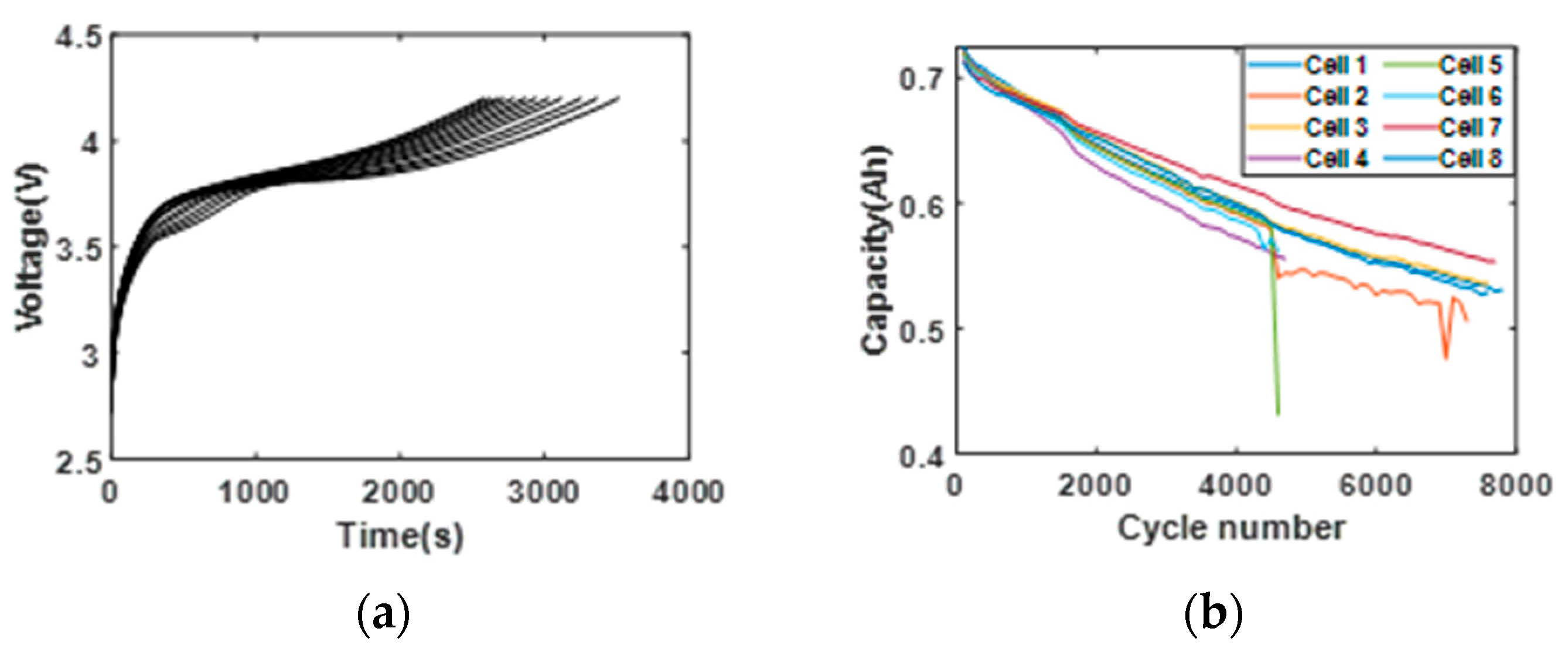The degradation data of a battery at different aging cycles from the Oxford dataset (the details are provided in Section 3.1) is used as an example. Firstly, the original V-Q curve ${\mathit{q}}_i$ is translated into a capacity sequence ${\tilde{\mathit{q}}}_i$ by introducing a voltage sequence $\mathit{V}={\left[V_i^{lo},V_i^{lo}+∆V,\dots ,V_i^{lo}+m∆V=V_i^{up}\right]}^T$, that is, ${\tilde{\mathit{q}}}_i={\left[q_i\left(V_i^{lo}+j∆V\right):j=0,\dots ,m\right]}^T$. Then, based on ${\tilde{\mathit{q}}}_i$, the matrix ${\mathbf{W}}_i$ is generated as follows:

$${\mathbf{W}}_i=\left[\begin{array}{ccc}∆q_{i,1}& \dots & ∆q_{i,m-2}\\ ∆q_{i,2}& \ddots & ∆q_{i,m-1}\\ ∆q_{i,3}& \dots & ∆q_{i,m}\end{array}\right],$$

(15)

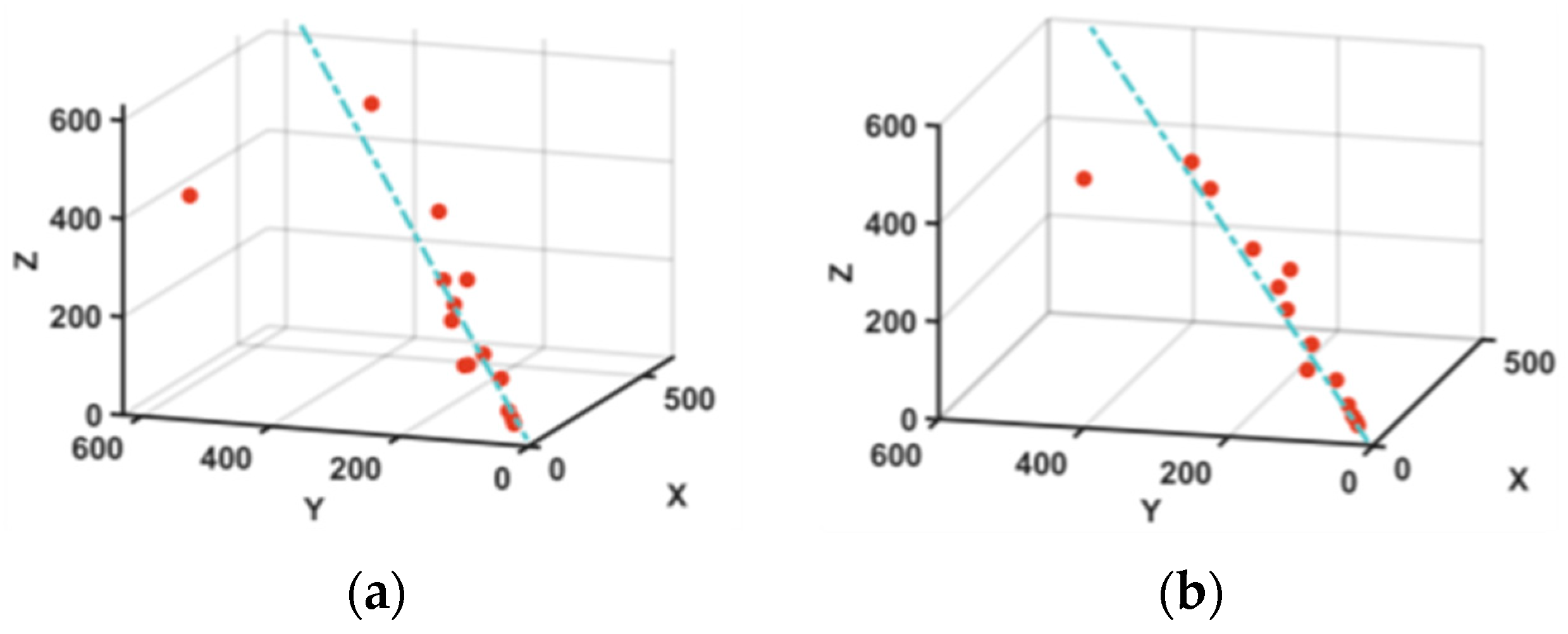
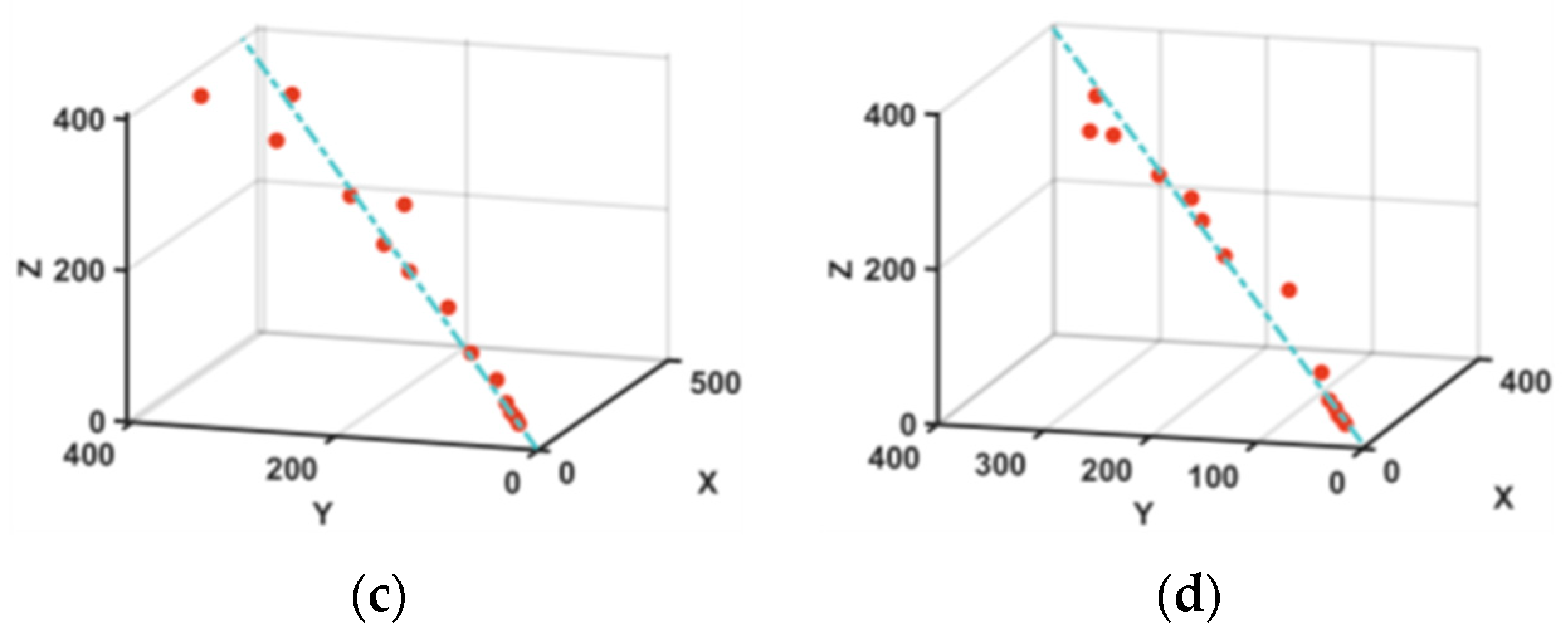
where $∆q_{i,j}=q_i\left(V_{lo}+j∆V\right)-q_i\left(V_{lo}+(j-1)∆V\right)$, $(j\in \{1,\dots ,m\left\}\right)$ is the capacity difference. Lastly, each column of ${\mathbf{W}}_i$ is taken as the coordinates of a 3D point to generate Figure 1. From each sub-figure, we can find the points generated with the data at a specific cycle distributed along a dominating direction. It is easy to see that the variation in $V_i^{lo}$ and $V_i^{up}$ does not affect the dominating direction but only changes the number of columns of matrix ${\mathbf{W}}_i$. In other words, no matter which part of the complete V-Q curve is collected, the generated points from matrix ${\mathbf{W}}_i$ always lie around the same line. Therefore, we propose to extract this feature as the input for our GP model.

To extract the dominating direction, principal component analysis (PCA) is introduced to decompose the matrix W_i by taking its columns as independent samples from 3D space. The results of PCA are presented in

Table 1. PCA results.

Cycle Number	1500	3000	4500	6000
First principal component	86.2%	92.8%	95.6%	95.9%
Second principal component	13.8%	7.2%	4.4%	4.1%

, from which we can find that the first principal component (PC) accounts for about 90% of the variation in different cycles. Thus, the first PC of matrix W_i, denoted as ${\mathit{z}}_i$, will be taken as the input at cycle $i$ for our GP model. It is worth noting that the construction of a valid W_i for PCA depends heavily on $V_i^{lo}$, $∆V$, and $m$. The sensitivity of the feature construction to these variables is evaluated in Section 4.

2.4. Scheme of Proposed Method

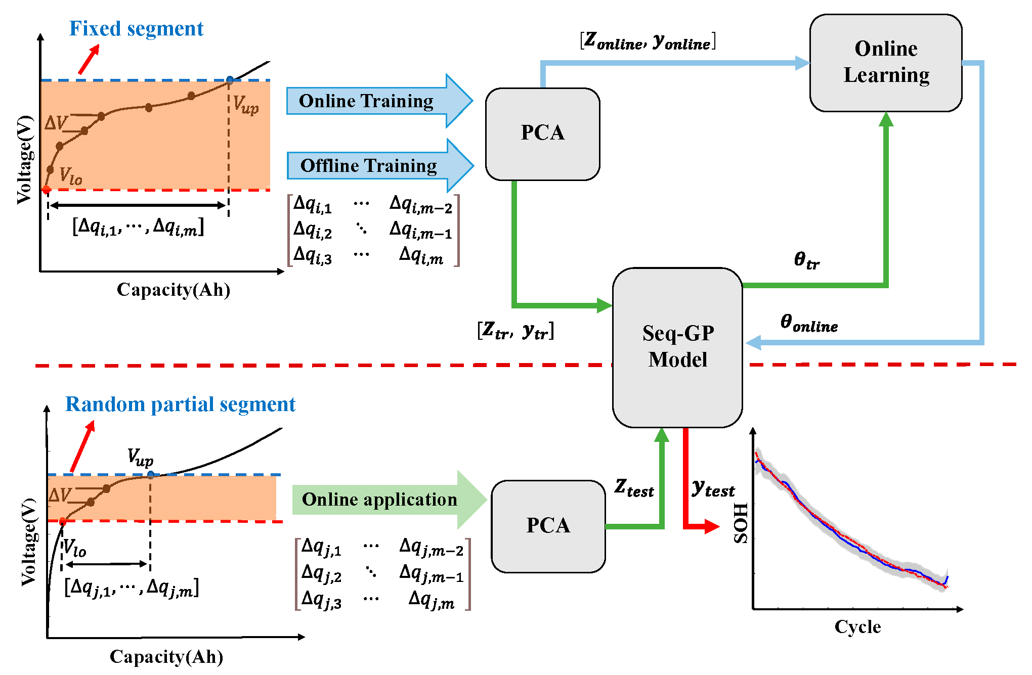
To summarize, our proposed SOH estimation procedure is shown in Figure 2. Firstly, based on the procedure introduced in Section 2.3, offline training inputs ${\mathit{Z}}_{tr}$ are constructed using historically collected V-Q curves. Secondly, the sequential GP proposed in Section 2.2 is trained with ${\mathit{Z}}_{tr}$ and observed SOH ${\mathit{y}}_{tr}$. After that, the trained model is used to estimate battery SOH based on the test features ${\mathit{Z}}_{test}$ constructed from random partial charging or discharging curves. Different from existing SOH estimation methods, during the online monitoring process, the model parameters in our method will be updated when newly collected data, i.e., $\{{\mathit{Z}}_{online},{\mathit{y}}_{online}\}$, are available. Through this updating process, the proposed method can reduce the computational complexity of GP-based models and, at the same time, incorporate information from new data to update model parameters, which enables better SOH estimation.

Importantly, the proposed feature extraction is compatible with fragmented charging scenarios. Unlike conventional methods requiring complete V-Q trajectories, our approach derives the dominating direction from local partial curves, with consistency validated across varying voltage intervals (Section 4.4). Combined with Seq-GP’s recursive update mechanism (Equations (11) and (12)), this enables streaming-mode operation without retraining on the entire historical dataset.

3. Experimental Setup

In this study, an aging test is carried out using two types of LIBs under different conditions to evaluate the proposed method under different datasets and aging conditions. An overview of each dataset is given in

Table 2. Overview of dataset information.

Dataset	Oxford	NASA
Form	Pouch	18650
Cell number	1–8	13–20
Capacity	0.74 Ah	2.1 Ah
Aging	All cell cycles with the same condition	Two groups, each with different conditions
Temperature	40 °C	25 °C

, and the experimental setup, including used LIBs, test protocols, etc., is presented below.

3.1. Aging Test Using Lithium-Ion Pouch Cell

The first dataset is the Oxford dataset, which is from the Oxford Battery Degradation Dataset1 [27]. It comprises experimental data on the aging of eight commercial Kokam pouch batteries. The batteries have a nominal capacity of 740 mAh, comprising graphite as the negative electrode material and lithium cobalt oxide/lithium nickel cobalt oxide as the positive electrode material.

During the experiments, the battery was subjected to a cycling process utilizing a Biologic MPG 205 constant potential meter and placed in a Binder MK 53 thermal chamber at a constant temperature of 40 degrees Celsius. Subsequently, the battery was subjected to an aging test utilizing a Binder MK 53 thermal chamber. The cycling procedure for the ageing experiments comprised repeated discharges employing ARTEMIS urban drive cycles and charging at a constant current of 2C. Following every 100 cycles, characterization tests were conducted, including full charge–discharge cycles at 1C. We utilized the charging curve data to construct the voltage profile, and Figure 3a illustrates the voltage curve of Cell 1 during the charging phase throughout its entire lifecycle. The battery capacity was calculated by integrating the IC charging curve. The calculated capacities of all eight batteries are plotted as a function of the number of cycles in Figure 3b.

3.2. Aging Test Using 18650 Li-Cobalt Cell

The second dataset is the NASA dataset, which is from the Prognostics Center of Excellence (PCoE) Randomized Battery Usage Repository at Ames Research Center [28]. The data in this repository are collected from the batteries under randomized load profiles so that they can better represent the batteries in real conditions. The experiments were conducted with 18650 Li-cobalt cells of 2.1 Ah, whose voltage ranges from 3.2 V to 4.2 V.

In this article, the last eight batteries in the repository were selected to validate the method. These batteries are from two groups, with each group undergoing a different randomized load profile, and the details are described in

Table 3. NASA dataset load profiles.

Group	Aging Condition
Group 1 (LIBs 13–16)	Four 18650 Li-ion batteries were continuously operated by repeatedly charging them to 4.2 V and then discharging them to 3.2 V using a randomized sequence of discharging currents between 0.5 A and 5 A. A customized probability distribution used to be skewed towards selecting lower currents was used to select a new load point every 1 min.
Group 2 (LIBs 17–20)	Same as group 1 except the probability distribution was used to skew towards selecting higher currents.

. After every 50 cycles, characterization measurements were taken, including a full 2 A charge–discharge cycle. Furthermore, different from the Oxford dataset, to demonstrate that our method can be used either in the charging or discharging phase, the discharge curves were used as the voltage curves. Figure 4a shows the voltage curves from Cell 20 during the discharging phase over its complete lifecycle. The capacity was calculated by integrating the 2-A charge curves. The calculated capacities for the batteries in the two groups are plotted against the cycle count in Figure 4b. Compared to Figure 3b, it can be observed that the capacity degradation trend is significantly affected by the battery type and working condition.

4. Results and Discussion

In this section, the battery SOH estimation performance of our proposed sequential GP (Seq-GP) is demonstrated through two case studies, and its accuracy and running time are compared with the regular GP (Reg-GP). To verify the accuracy of different methods, two different performance metrics, Mean Absolute Percentage Error (MAPE) and Root Mean Squared Error (RMSE), are applied in this paper.

4.1. Validation on the Same Aging Condition

The Oxford dataset is used to evaluate the performance of the model under the same aging cycle test conditions. It is worth mentioning that to simulate online application, the lower voltage limit $V_{lo}$ and the number of voltage segments $m$ selected in the testing process are different from those in the training process. In this section, lower voltage limits of different aging cycles in the testing process are randomly selected from the voltage range of 3.45–3.65 V, and the number of segments $m$ is set to 8, while the relevant parameters in the training process are shown in

Table 4. Parameters for offline training.

Dataset	Vlo (V)	Vup (V)	Delta V (mV)	m
Oxford	3.3	4.1	50	16
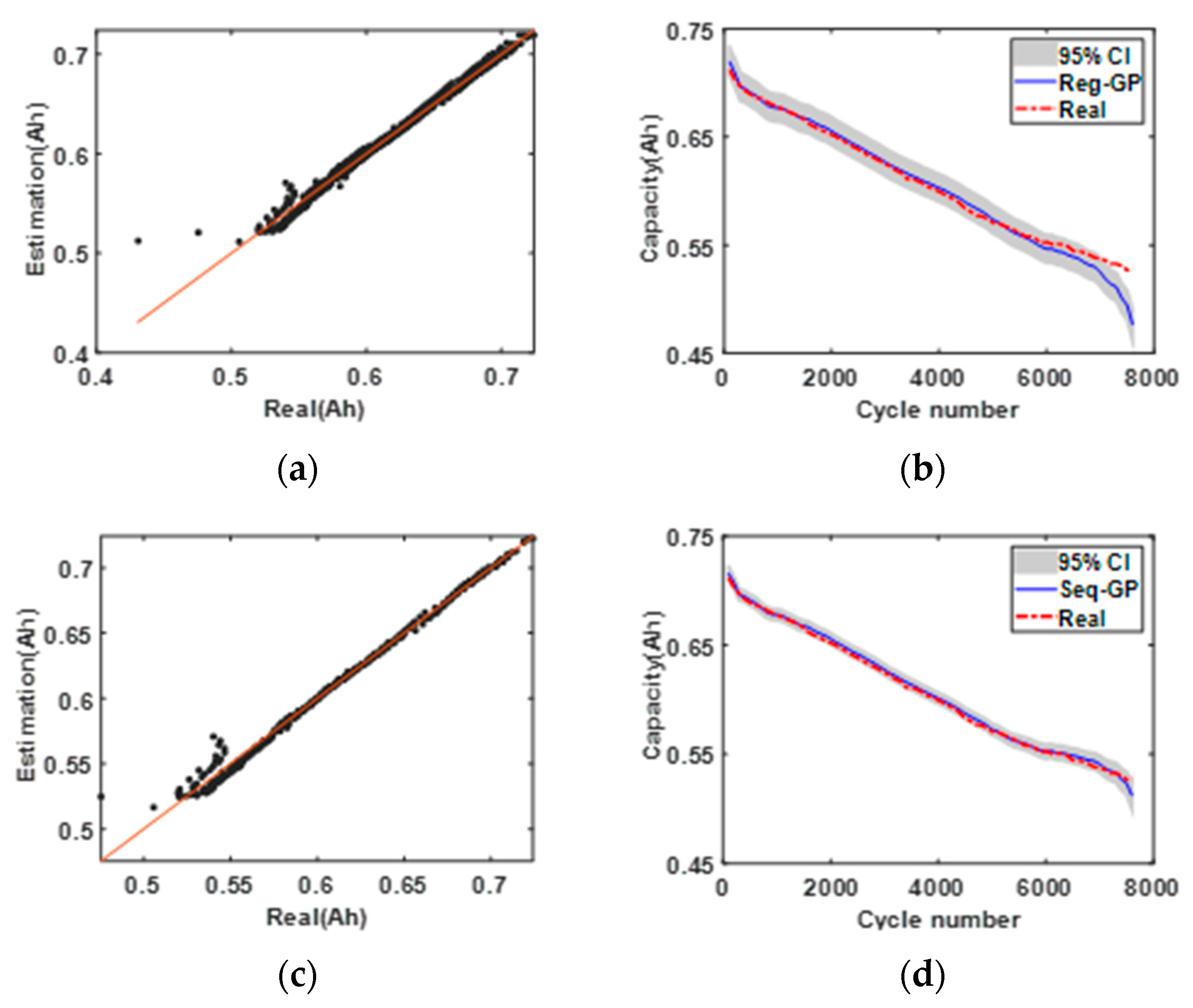
NASA	3.4	4.1	50	14

. For the 8 cells in the dataset, cells 1–4 are used as offline training datasets. Cells 5, 6, and 7 are considered as newly collected data for online updates, which is used to demonstrate that the proposed method has the capability to incorporate new data in an efficient way. The data of cell 8 is used for testing. Since online learning cannot be achieved with Reg-GP, the data of cells 1–7 are all utilized during the offline training process. As for the Seq-GP, the number of inducing points is set to 20. It should be noted that this number can also be optimized together with other model parameters. The SOH estimation results of Reg-GP and Seq-GP are shown in Figure 5, in which both the mean estimation and the 95% confidence interval (CI) are provided. The summary statistics are listed in

Table 5. Result statistics for the same aging condition.

Model	Reg-GP		Seq-GP
	Training	Testing	Training	Testing
RMSE(Ah)	0.0064	0.0096	0.0034	0.0035
MAPE	0.61%	0.98%	0.42%	0.44%
Time(s)	3.280	0.067	0.034	$4.69\times {10}^{-4}$

.

It can be observed that, by using the constructed features, both GP-based models can achieve sufficiently low training errors. For Reg-GP, RMSE and MAPE are 0.0064 and 0.61%, respectively, while for Seq-GP, RMSE and MAPE are only 0.0034 and 0.42%, respectively. This validates the effectiveness of the proposed input feature. However, it is worth noting that compared to Reg-GP, the training time of Seq-GP is reduced from 3.28 s to 0.034 s, which is a 98% decrease and validates the efficiency of the proposed method. During the testing process, RMSE and MAPE of Reg-GP increase to 0.0096 and 0.98%, respectively, which is adequate for actual application. Nevertheless, there is a slight flaw that Reg-GP cannot track the actual capacity aging trend particularly well when the aging cycle is over 6000 because of local nonlinear fluctuations. In comparison, by using the Seq-GP model, both the overall capacity trend and local nonlinear fluctuations are well fitted as desired in the test process. As for Seq-GP, its error in the test process is almost the same as its error in the training process, while its test time is also two orders of magnitude smaller than Reg-GP. This validates the efficiency and accuracy of the proposed method.

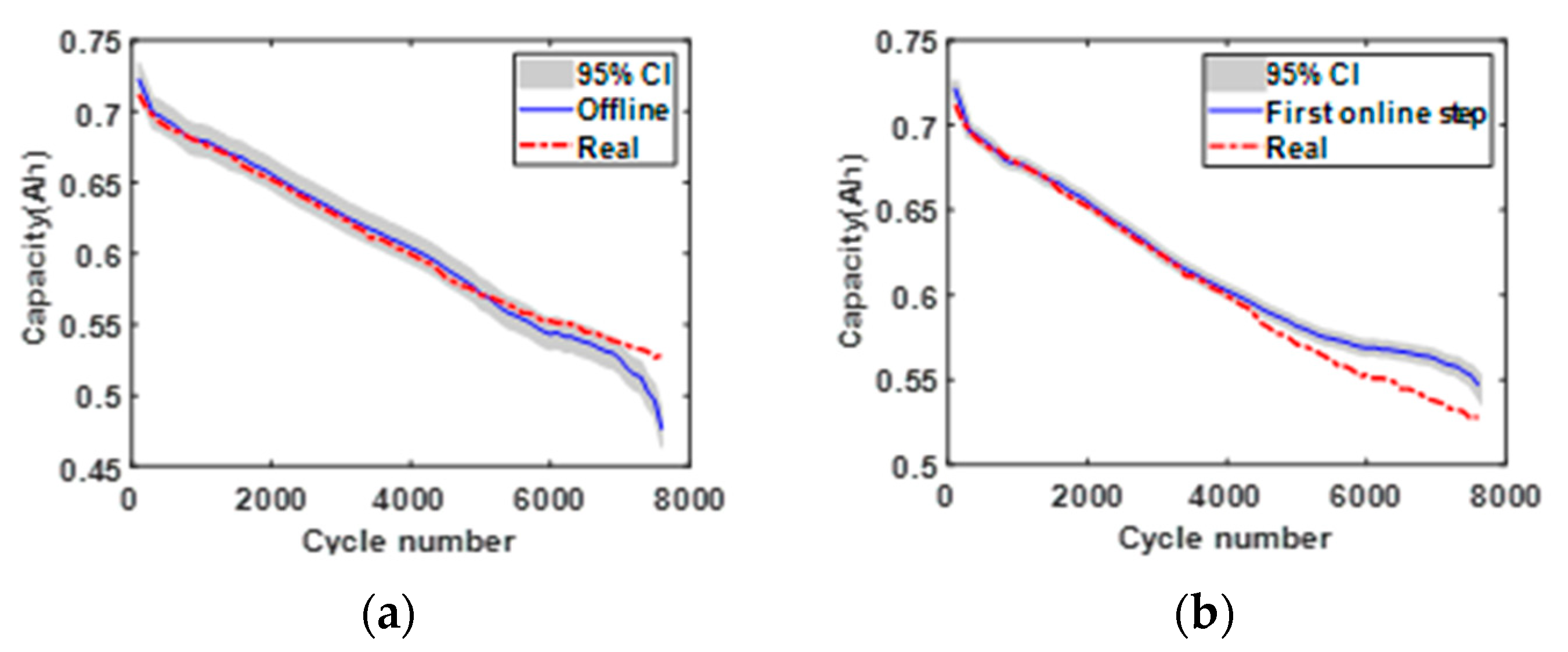
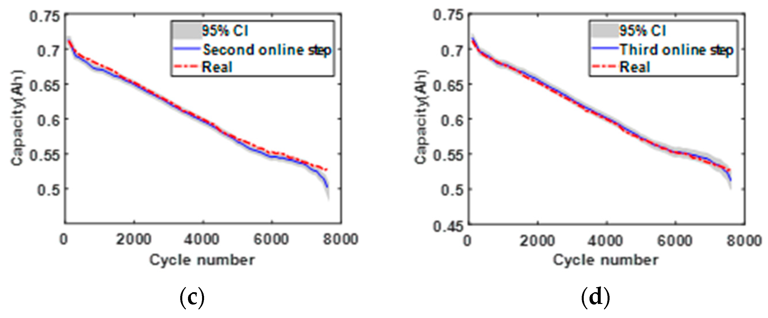
To further illustrate the online updating process of Seq-GP, Figure 6 shows the SOH estimation results after model updating four times. Figure 6a is the estimation result after offline training, while Figure 6b–d present the corresponding estimation results by adding cells 5, 6 and 7 as the online learning data. It suggests that there is an overall decreasing trend in the estimation error with the online update of model parameters. It is worth noting that the first online update step leads to a deteriorating performance due to the significantly different degradation path of cell 5 from other cells. In addition, the estimation CI becomes narrower as the update processes, indicating that the estimation becomes more reliable. Therefore, in terms of the above results, it can be concluded that Seq-GP is effective and highly accurate for battery SOH estimation when the cells age under the same condition.

4.2. Validation on the Dynamic Aging Condition

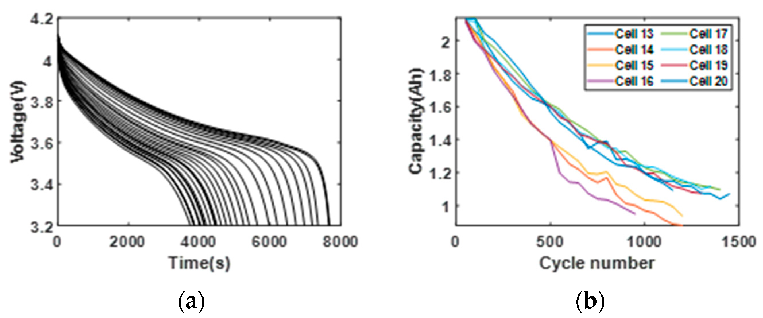
To further evaluate the proposed model under dynamic aging conditions, two groups of NASA datasets with different aging conditions are used to evaluate the performance. As described in Section 3.2 and Table 3, cells 13–16 were cycled with a lower-current randomized load profile, whereas cells 17–20 were cycled with a higher-current randomized load profile. In this section, for Seq-GP, cells 13–16 are used as offline training datasets, cells 17–19 are used as training sets for the online updating process, and cell 20 is used as the testing data. As for Reg-GP, cells 13–19 are all used during the offline training process. In addition, the number of inducing points for Seq-GP is set to 10 since the number of aging samples in the NASA dataset is less than that in the Oxford dataset, while other parameter settings are consistent with the Oxford dataset. Notably, the NASA dataset contains randomized dynamic loading profiles: the discharging current is randomly selected between 0.5 A and 5 A at one-minute intervals (Table 3), representing non-constant-current battery aging data. Testing under this randomized dynamic loading profile further demonstrates the adaptability of the proposed method under a different aging protocol.

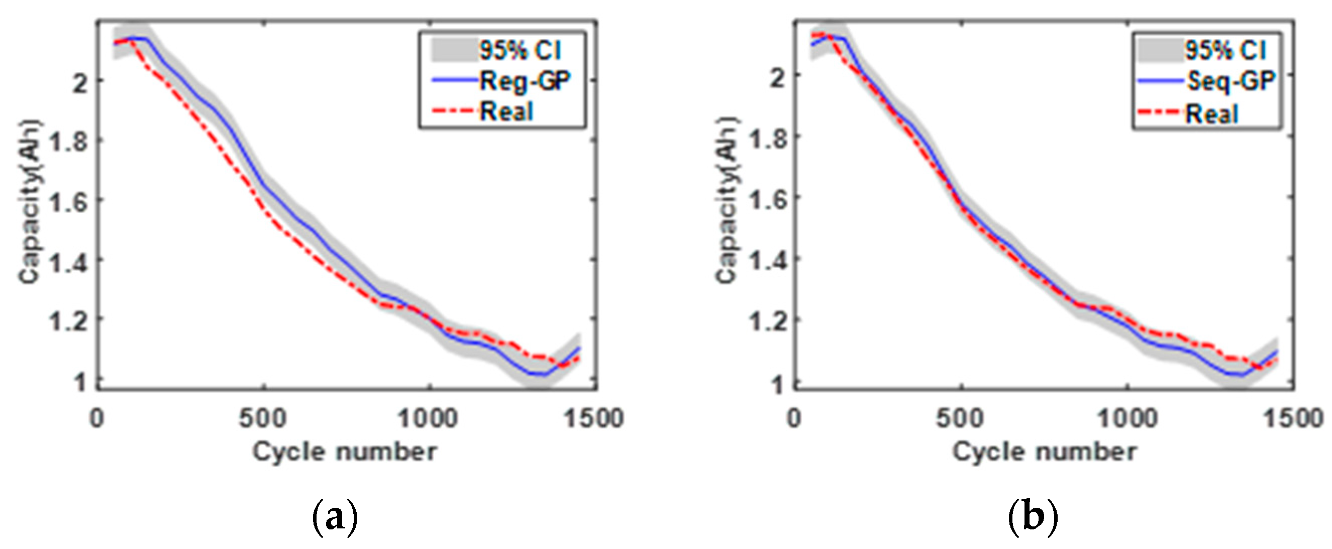
The estimation results are shown in

Table 6. Result statistics for dynamic aging conditions.

Model	Reg-GP	Seq-GP
RMSE(Ah)	0.0609	0.0317
MAPE	3.56%	1.96%
Training time(s)	0.4799	0.0537
Test time(s)	3.40 × 10−3	4.20 × 10−4

and Figure 7. It can be seen that the estimation from Seq-GP matches the actual data well, while the obtained 95% CI of Reg-GP cannot cover the overall degradation trend during most of the aging cycles. The main reason leading to the low estimation accuracy of Reg-GP is that the aging trends of the two groups are different from each other. In comparison, Seq-GP captures the capacity degradation trend well, with the RMSE as 0.0317 and MAPE as 1.96%, which are only half of those from Reg-GP. In addition, the training and testing times of Seq-GP are also significantly lower than those of Reg-GP.

In a nutshell, the NASA dataset presents a greater challenge for SOH estimation due to the different cycling regimes for the two groups of cells. Moreover, even for each group, the cells are cycled with dynamic loading profiles during their aging process. Nevertheless, the proposed model can still achieve accurate estimation results with lower computational complexity. In conclusion, these facts signify that, even for dynamic aging conditions, Seq-GP also delivers reliable and accurate estimation results.

4.3. Comparison with Alternative Data-Driven Methods

To further validate the proposed Seq-GP, three widely adopted data-driven methods are implemented for comparison under the stated PCA-feature-based comparison protocol: Support Vector Regression (SVR), a Convolutional Neural Network (CNN), and a Long Short-Term Memory network (LSTM). All three methods share the same PCA-based input features (Section 2.3) and train/test splits as described in Section 4.1 and Section 4.2. The comparison is summarized in

Table 7. Comparison of estimation accuracy with alternative data-driven methods.

Methods	Online Update	Uncertainty	Oxford		NASA
			RMSE (Ah)	MAPE (%)	RMSE (Ah)	MAPE (%)
Seq-GP	Yes	Yes	0.0035	0.44	0.0317	1.96
Reg-GP	No	Yes	0.0096	0.98	0.0609	3.56
SVR	No	No	0.0067	0.65	0.0355	3.43
CNN	No	No	0.0194	1.74	0.0578	4.04
LSTM	No	No	0.0107	1.13	0.0325	3.30

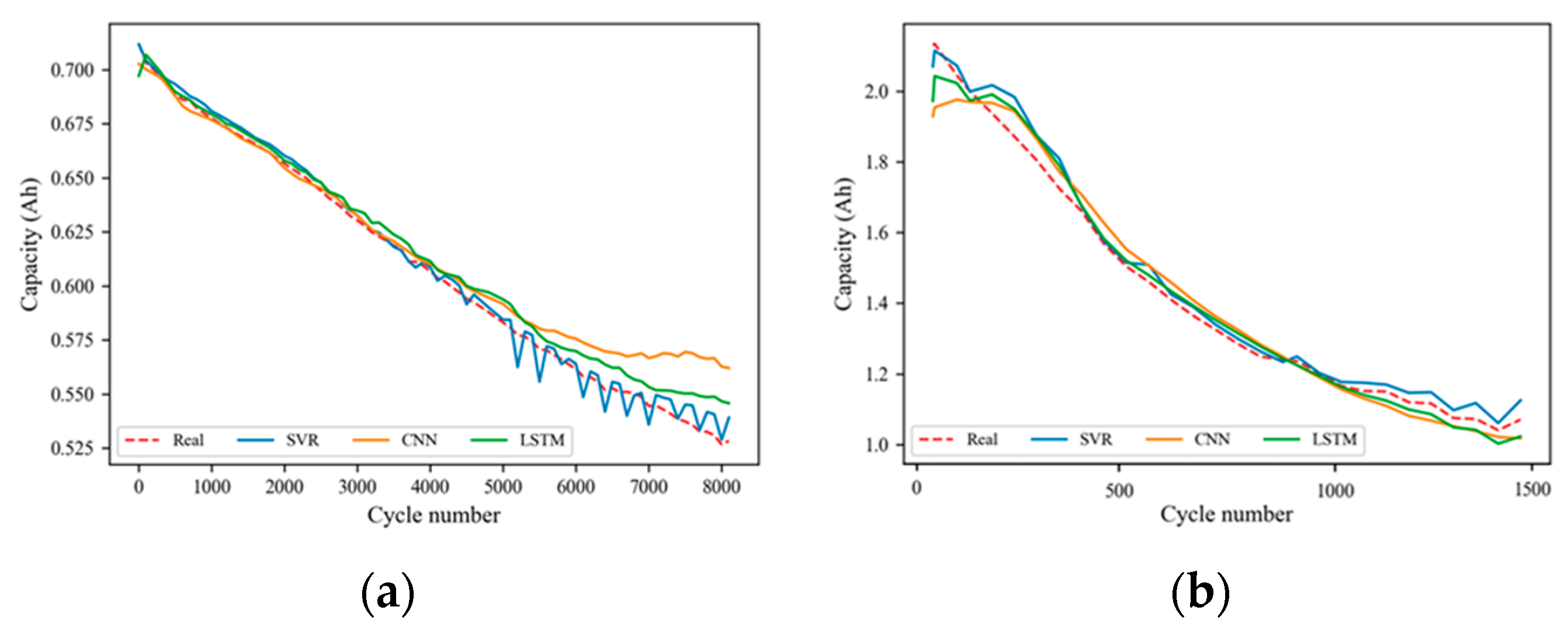
, where the Reg-GP and Seq-GP entries are quoted directly from Table 5 and Table 6. Figure 8 visualizes the test-set predictions of the three alternative methods against the measured capacity for both datasets.

Under the tested PCA-feature-based comparison protocol, Seq-GP achieves the lowest errors among the evaluated implementations on the Oxford dataset, followed by SVR, LSTM, and CNN. On the NASA dataset, Seq-GP also yields the lowest errors among the tested methods, while the alternative models show larger deviations under the randomized dynamic loading condition, particularly at later aging cycles where the V-Q curves exhibit greater variability. The training times of the alternative methods are considerably longer than those of Seq-GP (0.034 s): SVR requires 1.45 s, LSTM 7.02 s, and CNN 33.7 s, owing to the iterative gradient-based optimization inherent in neural network training.

More importantly, none of the three alternatives support online parameter updating or principled uncertainty quantification. The ability to sequentially incorporate new data without retraining and to provide confidence intervals for each prediction is inherent to the GP framework and essential for practical BMS deployment. Within the standard SVR, CNN, and LSTM implementations evaluated here, Seq-GP additionally provides online posterior updating and predictive uncertainty quantification. These results support its suitability for the stated online SOH estimation workflow, while broader benchmarking against specialized partial-curve methods remains a direction for future work.

4.4. Influence of the Lower Voltage Limit

As described in Section 4.1, the lower voltage limit is randomly selected during the testing process. Hence, the influence of the lower voltage limit is investigated using the Oxford dataset by varying the limit from 3.35 V to 3.65 V. The estimation error of Seq-GP with different lower voltage limits is presented in Figure 9 with $m=8$ and $\mathsf{\Delta }V=50 \mathrm{m}\mathrm{V}$. 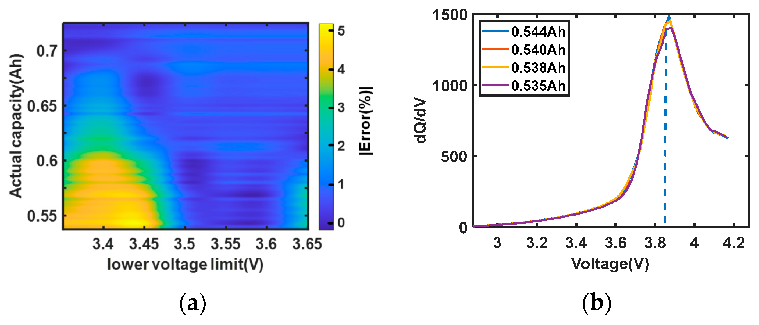As illustrated in Figure 9a, the estimation error is bounded by 5.09% and the average error is 1.28%. Interestingly, large errors are mainly concentrated in the area where the lower voltage limit is less than 3.45 V. The possible reason for this can be explained by the IC curves plotted in Figure 9b. According to previous research [18], the peak of the IC curve includes valuable information for the degradation of LIBs. Thus, when the voltage segment includes the interval where the IC peak occurs, the estimation error will be small. It is clear from Figure 9b that the peaks of IC curves at different aging cycles are located around 3.85 V. However, when the lower voltage is smaller than 3.45 V, the upper voltage limit is less than 3.85 V of the Oxford dataset with $m=8$ and $\mathsf{\Delta }V=50 \mathrm{m}\mathrm{V}$. Within the voltage interval between 3.45 V and 3.85 V, no representative features can be obtained, which explains the large error area located in the region where the lower voltage limit is less than 3.45 V. In general, there is a slight difference in the estimation accuracy of the proposed method under different lower voltage limits, which supports the stability of Seq-GP within the tested lower voltage range.

4.5. Influence of the Number of Segments

When the lower voltage limit is given, the value of the upper voltage limit is determined by the number of segments $m$. Thus, it is necessary to investigate the effect of the number of segments on the estimation accuracy. In this section, the lower voltage limit is set to 3.5 V and the estimation result for the Oxford dataset is shown by varying $m$ from 6 to 14 in Figure 10. 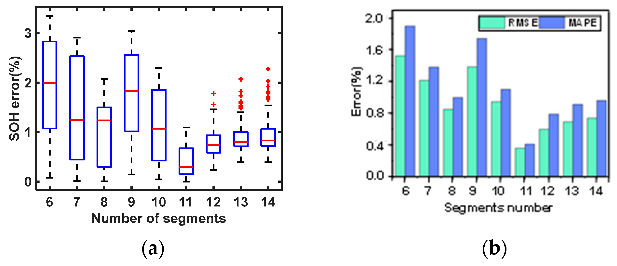It can be seen from Figure 10a that the median estimation error is consistently lower than 3% with the increase in $m$, which indicates stable performance across the tested segment numbers. Moreover, the error reaches a local minimum with MAPE of 0.99% and normalized RMSE of 0.85% when $m$ reaches 8. For practical applications, the value of $m$ should be as small as possible since a smaller $m$ indicates a narrower voltage segment. Considering both the accuracy and the voltage range, it is recommended to choose $m=8$.

4.6. Discussion on Real-World BMS Implementation Feasibility

While the preceding results validate the accuracy of the Seq-GP, it is also necessary to assess its viability under the hardware and operational constraints of commercial Battery Management Systems, particularly for electric vehicles. In contrast to regular GP, whose complexity scales cubically with all historical data, the complexity of Seq-GP is primarily governed by the number of inducing points $n_{\mathcal{U}}$, yielding a complexity of $\mathcal{O}\left(n_{\mathcal{U}}^3\right)$ and a memory footprint of $\mathcal{O}\left(n_{\mathcal{U}}^2\right)$. In our implementation, $n_{\mathcal{U}}$ is set to 20 for the Oxford dataset and 10 for the NASA dataset, which translates to matrix inversions of size 10 × 10 to 20 × 20 only, requiring less than 0.05 s and less than 2 KB of RAM on a typical 32-bit microcontroller. These specifications are well within the capabilities of modern automotive BMS controllers.

It is also worth clarifying that the online update does not require continuous recursive computation during high-frequency current sampling. Instead, the model parameters are stored in non-volatile memory and updated only when a new partial charging or discharging segment is completed, such as at the end of a daily commute or a charging session. This event-driven mechanism ensures that computational resources are not contended with real-time safety-critical tasks. Moreover, a practical advantage of our feature extraction method is that it does not rely on full 0–100% SOC cycles, which are rarely seen in actual EV usage. The PCA-based feature maintains a consistent dominating direction regardless of the starting voltage limit, making it adaptable to erratic driving and charging profiles, while also attenuating high-frequency sensor noise. These characteristics indicate that Seq-GP has practical potential for onboard SOH estimation in BMS applications, while validation using real-world onboard data remains an important next step.

4.7. Applicability and Limitations Regarding Battery Chemistries

The GP regression backbone is not tied to a specific battery chemistry, as it serves as a general Bayesian nonparametric regressor that learns the mapping between constructed features and SOH. In this study, we validated its effectiveness on two representative chemistries—Kokam pouch cells (LCO/NMC) and 18650 Li-Co cells—under both steady and dynamic aging protocols. The consistently low estimation errors and narrow confidence intervals observed in these two datasets demonstrate the adaptability of the online updating mechanism under the tested operating conditions.

However, we recognize that the current feature construction method—which relies on the dominating direction extracted from capacity difference matrices—may require careful reconsideration when applied to batteries with intrinsically flat voltage profiles, such as LiFePO₄ (LFP) cells. In such cases, the small variation in capacity difference across the plateau region could reduce the discriminative power of PCA-based features. Importantly, this is not a limitation of the Seq-GP algorithm, but rather a stimulus for future innovation in feature engineering. Our ongoing work is investigating two promising avenues to address this: (1) transforming the voltage axis into the incremental capacity (dQ/dV) domain to amplify degradation signals even under plateau conditions, and (2) employing functional data analysis to directly model the entire partial curve as a functional input, thereby bypassing the need for hand-crafted features.

Therefore, we maintain that Seq-GP offers an efficient online Bayesian updating backbone for SOH estimation, while its compatibility with diverse chemistries can be further strengthened through adaptable feature extraction strategies—a direction we explicitly highlight for future research.

5. Conclusions

In this paper, a data-driven method, i.e., Seq-GP, is proposed with the construction of a novel input feature for the online SOH estimation of LIBs, targeting the challenges of online model updating and partial V-Q curves in real-world applications. Specifically, a variational sparse approximation technique is introduced to realize efficient online updating of the proposed GP model. In addition, to deal with the random parts of V-Q curves during real operation, the dominating pattern of the capacity sequence is extracted as the input for Seq-GP to achieve accurate SOH estimation. The effectiveness of our method is validated by two different datasets with various aging conditions. The sequentially updating nature of our method provides both improved estimation accuracy and significantly reduced computational cost compared to conventional GP. Its effectiveness has been demonstrated across two distinct battery chemistries and multiple aging protocols, including both constant-current and randomized dynamic loading profiles. Furthermore, the adaptability of the proposed framework to other chemistries, such as LiFePO₄, is discussed as a promising direction for extending the current feature engineering module, rather than a fundamental barrier to the method’s applicability.

There are still some open questions that can be further investigated. Firstly, the matrix ${\mathbf{W}}_{\mathrm{i}}$ is constructed with the difference in capacity values, which may not be appropriate for LiFePO₄ batteries due to the voltage plateau in the V-Q curve. In the future, functional data analysis can be introduced to construct more versatile inputs from the partial charging or discharging data. Secondly, the extension of the proposed Seq-GP for battery modules would also be an interesting research topic in the future. While our method performs well on standardized laboratory datasets, on-vehicle validation under naturalistic driving conditions remains the next critical step. Future work will implement Seq-GP on an embedded BMS platform for evaluation using real-world onboard data streams.