State of Health Estimation of a Lithium-Ion Battery Used in a Trolleybus Under Real Operating Conditions

Abstract

Battery use in trolleybuses improves energy efficiency and enables driving outside routes with overhead contact lines. This paper analyses the ageing process of lithium-ion batteries by determining the State of Heath (SOH) curve based on real-world data collected during six and a half years of trolleybus operation. The battery, manufactured using NMC technology (lithium-nickel-manganese-cobalt LiNiMnCoO₂), was used as an onboard energy storage unit. The battery pack powers the trolleybus on the non-electrified route segments and improves its energy efficiency. In this paper, the ageing process of the lithium-ion battery in such a vehicle was investigated, using recorded data for each day of operation between 2016 and 2023. The SOH of the battery was estimated on the basis of three criteria: specific SOC range, specific battery voltage range and specific battery pack temperature range. Under these circumstances, the values of electric charge and energy flow into the battery were analysed, allowing the obtainment of the battery SOH value. Empirical distributions of random variables related to the minimum and maximum battery temperature and battery discharge current were presented. Based on these empirical distributions, statistical descriptors representing health indicators were calculated. The environmental factors (temperature, SOC, discharge and charge currents) that had a significant impact on the ageing process of the battery under test were analysed as well.

1. Introduction

Equipping trolleybuses with an onboard energy storage unit is the result of multi-criteria planning of the public transport service, with the consideration of energy efficiency in agglomerations that have trolleybus infrastructure [1]. The advantages of using batteries in trolleybuses include increased energy efficiency, off-wire operation and in-motion charging.

The data acquisition system in modern, electrochemical storage-equipped trolleybuses records several dozen analogue and digital signals in the real time. From the point of view of energy efficiency of the electric vehicle (EV), the basic dataset recorded in battery-equipped trolleybus contains parameters such as:

• Time in a specific format (YY.MM.DD.hh.mm.ss);
• Vehicle identifier;
• Energy consumed by the drivetrain (kWh);
• Energy of the regenerative braking generated by the drivetrain (kWh);
• Energy fed from the overhead catenary (kWh);
• Energy regenerated into the overhead catenary (kWh);
• Operation in battery mode—Battery Mode;
• Operation in catenary mode—Catenary Mode;
• Distance covered (km);
• Inside and outside temperature (C);
• Velocity (km/h);
• GPS coordinates of the vehicle (latitude and longitude);
• Passenger room air conditioning status;
• Traction battery SOC (%);
• Line voltage (V);
• Line current (A);
• Minimal (MinTemp) and maximal (MaxTemp) temperature of the battery pack.

A single dataset contains data recorded during one day of service, i.e., from 00:00 to 23:59. Sampling of the data acquisition is dependent on the energy management system (EMS) used in the electric vehicle [2]. Typically, in electric vehicles two methods are used for data acquisition: constant distance step or constant time step when the vehicle is stopped and variable (velocity-dependent) time step when the vehicle is in motion. The size of the dataset recorded during one hour or one day depends on multiple factors, including data resolution (analogue signals), sampling frequency and saving format (binary or text). For the recording of data mentioned above and variable time step, a single file size is around 10 MB per day, if the data is saved in the text format. The dataset used for analysis presented in this work has been obtained from the public transportation company, operating in one of the northern countries of the European Union. Recorded data is organised in tables that are saved in files with specific signatures and archived on dedicated servers, constituting the database entries.

The size of the dataset collected for each trolleybus during the span of a few years is relatively large. Considering the size of the trolleybus fleet, such datasets could be categorised as Big Data (BD). Processing of the data contained in such databases is carried out using dedicated software. For this task, SQL (Structured Query Language) is used extensively. It is a relatively simple and efficient programming language, designed specifically for accessing, processing and modifying entries of relational databases. SQL was developed in 1974 and it is still the universal programming language used in data processing and complex report generation.

Advancements in Big Data prompted the development of multiple tools dedicated to database processing. One such tool is the Language Integrated Query (LINQ). In relation to SQL, LINQ is simpler, more efficient and more advanced [3,4,5]. In this paper, the authors implemented LINQ-based queries for processing and analysing data obtained from a single trolleybus. The software developed for this purpose is described in [6], which provides a detailed explanation of how to create a query with specific criteria regarding the SOC, voltage, current and temperature of the battery.

The object of the analysis is a Solaris Trollino 12 M (3rd generation) trolleybus, with an identifier ID = 3088. The nominal capacity of the battery pack C = 62 Ah (according to the manufacturer data, ENERDEL), containing 14 12S2P-type cells.

Analysis features data recorded between 1 January 2016 and 30 June 2023 (six and a half years of operation). Each battery module in the pack is equipped with a temperature sensor. The battery management system measures the temperatures of all modules, but only the minimum and maximum temperatures are recorded in the database. Differences were observed between the extreme temperature values, indicating that the modules were not operating at the same temperature and there was some temperature distribution throughout the pack.

Estimation of the battery SOH is typically done using various battery fade models. Such models can be divided into three groups, as presented in [7,8,9]: (1) model-based approach (MBA), (2) data-driven approach (DDA) and (3) hybrid approach (HA). Most studies on battery SOH models are based on laboratory data obtained under controlled conditions and do not take into account the variability of a number of parameters (temperature, current, SOC, DOD, etc.) occurring in the actual operating conditions of the vehicle. In the real operating conditions of an electric vehicle providing a public transport service, it should be expected that a number of parameters such as temperature, current, voltage, SOC, etc. are characterised by certain statistical distributions. As the battery operation time increases, the random variables of the relevant parameters are more representative in the battery SOH assessment. Developing reliable SOH models based on a data-driven approach requires testing or training them on at least several years of historical data obtained from a real-world data on battery operation.

In [10], the framework for the analysis of the remaining driving range (indirectly related to the SOH) for passenger car and bus fleets in different cities over a three-year period was verified. The buses were equipped with a LiFePO4 battery, while the electric passenger vehicles were equipped with an NMC battery. The dynamics of the ageing process between an NMC battery (analysed in this work) and an LFP battery are not the same, because in the LFP battery the degradation process is more stable, more uniform, and less sensitive to temperature. The conclusions regarding electric passenger cars with NMC batteries indicate a very significant influence of the energy consumption rate, which is closely related to the driving style and, consequently, the SOH deterioration process.

The new battery ageing phenomenon presented in [11] is based on historical data from electric buses stored in a memory cloud. To verify the effectiveness of the proposed modelling method, an LFP battery with a nominal capacity of approximately 200 kWh was used, which, as indicated earlier, is characterised by a different dynamic of the battery ageing process than an NMC battery.

In [12], a universal feature extraction framework developed for estimating the SOH is presented, which can be applied to NMC and LFP batteries. Real-world data from 3 years of operation of electric vehicles was analysed. Data for model testing was collected from 17 cars with NMC batteries and 20 cars with LFP batteries. It was concluded that the SOH estimation models are representative for NMC and LFP batteries, but the limited variety of vehicle types makes it difficult to assess the generalisability of the SOH model to other vehicles.

In [13], historical data was used to estimate the SOH of a lithium-ion battery and also to predict the SOH depending on future load information. The tested battery (a pack of six 18,650 Li-ion batteries with a rated capacity of 2.1 Ah) was a relatively small energy storage unit that was tested using a discharge pattern called a random walk (RW) profile. These types of tests are performed on single lithium-ion cells used in NASA’s “Random Battery Use” experiments. In this NASA battery ageing experiment, the temperature was controlled and set near room temperature. NASA RW test results can be helpful in estimating SOH, but cannot be used as a direct substitute for real EV data.

The real-world dataset used in [14] comprises 20 commercial electric vehicles equipped with NMC batteries that were continuously monitored for approximately 29 months to estimate the SOH degradation rate based on real-time frequent itemset image encoding. In this study, the data sampling rate was relatively high, at 8 s. This is sufficient for monitoring SOC values to estimate SOH. However, such a high sampling rate is not suitable for monitoring instantaneous battery currents and voltages in real electric vehicles, which are used for SOH estimation.

In [15], a detailed study on SOH estimation was presented, including the collection of real data from 860 electric vehicles equipped with NMC batteries, operated in real conditions for 4 years. This study analysed direct parameters such as battery voltage, current and temperature, as well as cumulative total capacity, total charging energy and total mileage. The developed GAM-FNN (Grouped Attention Mechanism-FNN) framework improves the accuracy of SOH estimation for electric vehicles. Unfortunately, the SOH model developed for electric passenger vehicle NMC batteries cannot be directly applied to trolleybus batteries due to different load profiles, temperatures and degradation patterns.

The most important factor in the operation of an electric vehicle, especially an electric bus or trolleybus, is the prediction of the time interval of the mid-life degradation curve. As the time span of historical data increases, the SOH and RUL estimation becomes more stable and more predictable. This paper presents the SOH estimation of the NMC battery pack based on a dataset obtained from historical data, covering a timespan of six and a half years of trolleybus operation. A data-driven approach is used, including direct parameters such as battery voltage and current, minimum and maximum battery temperature in the pack, and the SOC to estimate the battery SOH. Some statistical descriptive methods were used to determine the battery health indicators (HIs) based on current and temperature data. In the case of relatively long trolleybus operation, the selection of representative HIs is essential for accurate SOH estimation, and statistical features are among the commonly used categories in SOH estimation.

The main contributions of this study include:

• Data from six and a half years of operation of a trolleybus providing a public transport service in real conditions were pre-processed in order to prepare them for estimating the SOH of the NMC battery pack.
• The SOC specific interval and battery voltage specific interval methods to estimate SOH were used to collect the battery data subset corresponding to the SOC criterion and the battery voltage criterion. The extracted data subset covers six and a half years of trolleybus operation.
• A statistical analysis of the charge drawn from the battery in the Motoring mode of operation of the trolleybus drive system was performed. The charge drawn from the battery consists of two components. The first component, designated Q1C, corresponds to a battery discharge current of up to 1C. The second component, designated QOC, corresponds to a battery discharge current above 1C. The statistical distributions of the Q1C, QOC and QOC/Q1C ratio have been determined as new battery health indicators.
• The statistical distributions of the minimum and maximum battery temperatures that constitute the battery stack are determined, and important distribution-based metrics as battery health indicators are also given.
• Mathematical formulas for the SOH of the NMC battery pack were derived in the form of polynomials in the time domain of trolleybus operation, which correspond to the determined statistical distributions. The SOH formula based on the SOC criterion and the SOH formula based on the battery voltage criterion give very similar results.

The paper is organised as follows. In Section 2 of this work, selected histograms presenting relative values of energy regenerated into the catenary, drivetrain regenerative braking energy and distance covered under battery power are shown. Section 3 contains selected waveforms of energies, voltages, currents, distance, velocity etc. during the one day of the vehicle operation. In Section 4, criteria used to determine battery SOH as well as figures of energy and electrical charge stored in the battery were discussed in the historical context. In Section 5, degradation factors of the traction battery were discussed in the context of the energy storage equipped in the analysed vehicle. Section 6 contains results of the SOH obtained under specified criteria. In Section 7, obtained results were summarised.

2. Histograms of the Selected Random Variables of the Vehicle

In this section, empirical distributions of selected quantitative characteristics related to one day of trolleybus operation during the data analysis period (1 January 2016–30 June 2023) are presented. Such quantitative characteristics and distributions are:

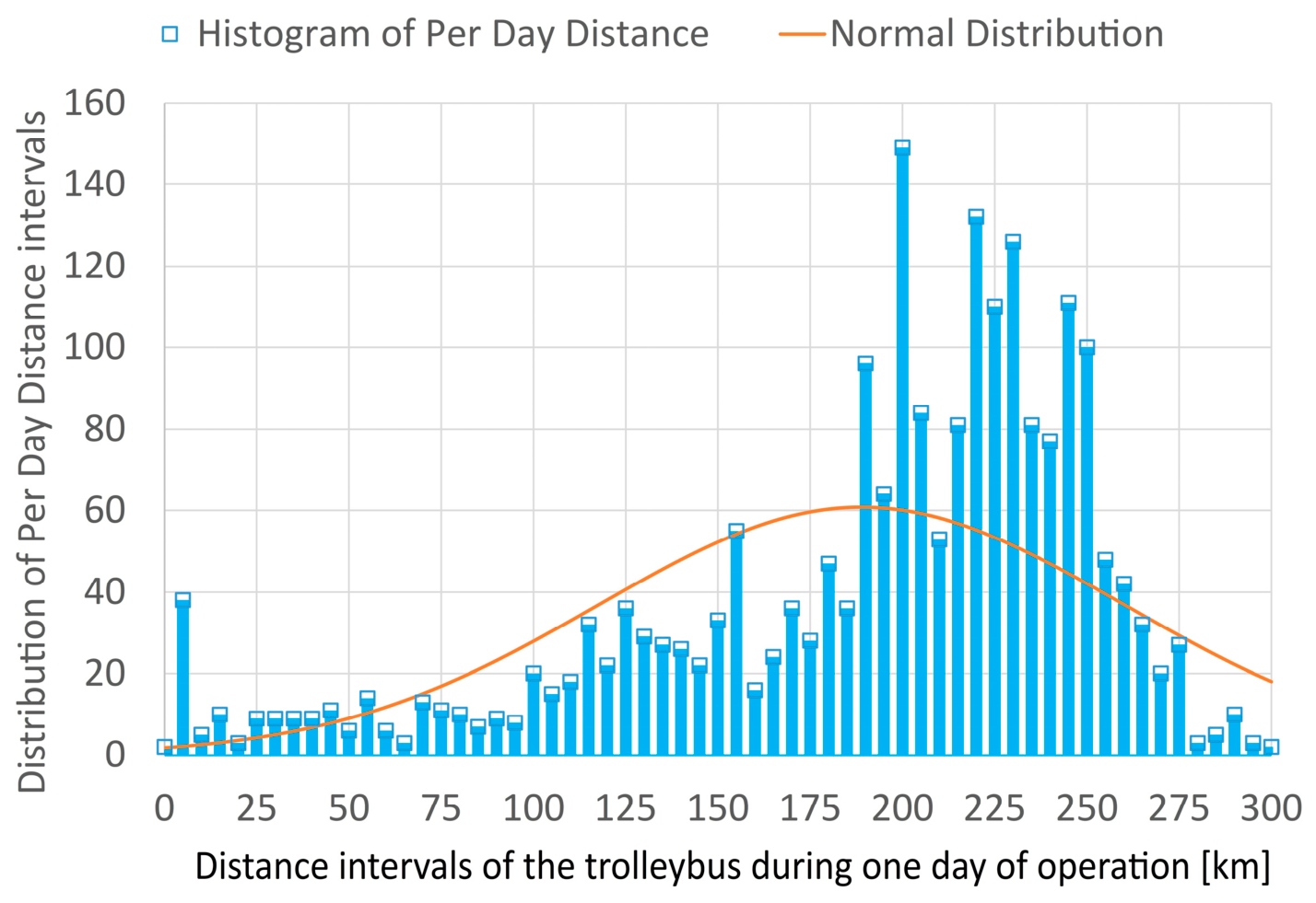
• Distance covered by the vehicle during a single day—Histogram PerDayDistance—Figure 1;
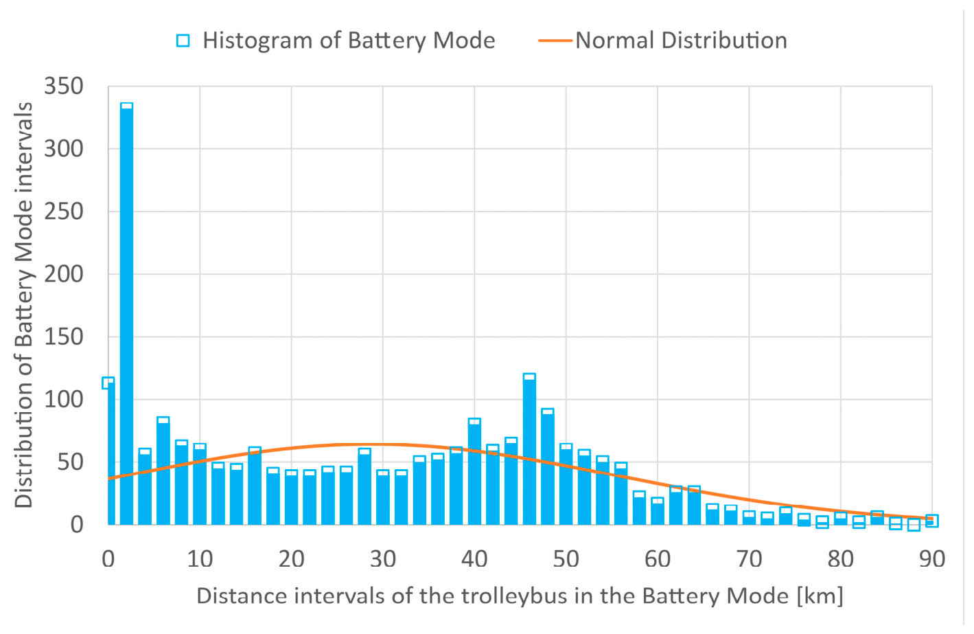
• Distance covered by the vehicle in the battery operation mode—Histogram BatteryDistance—Figure 2;
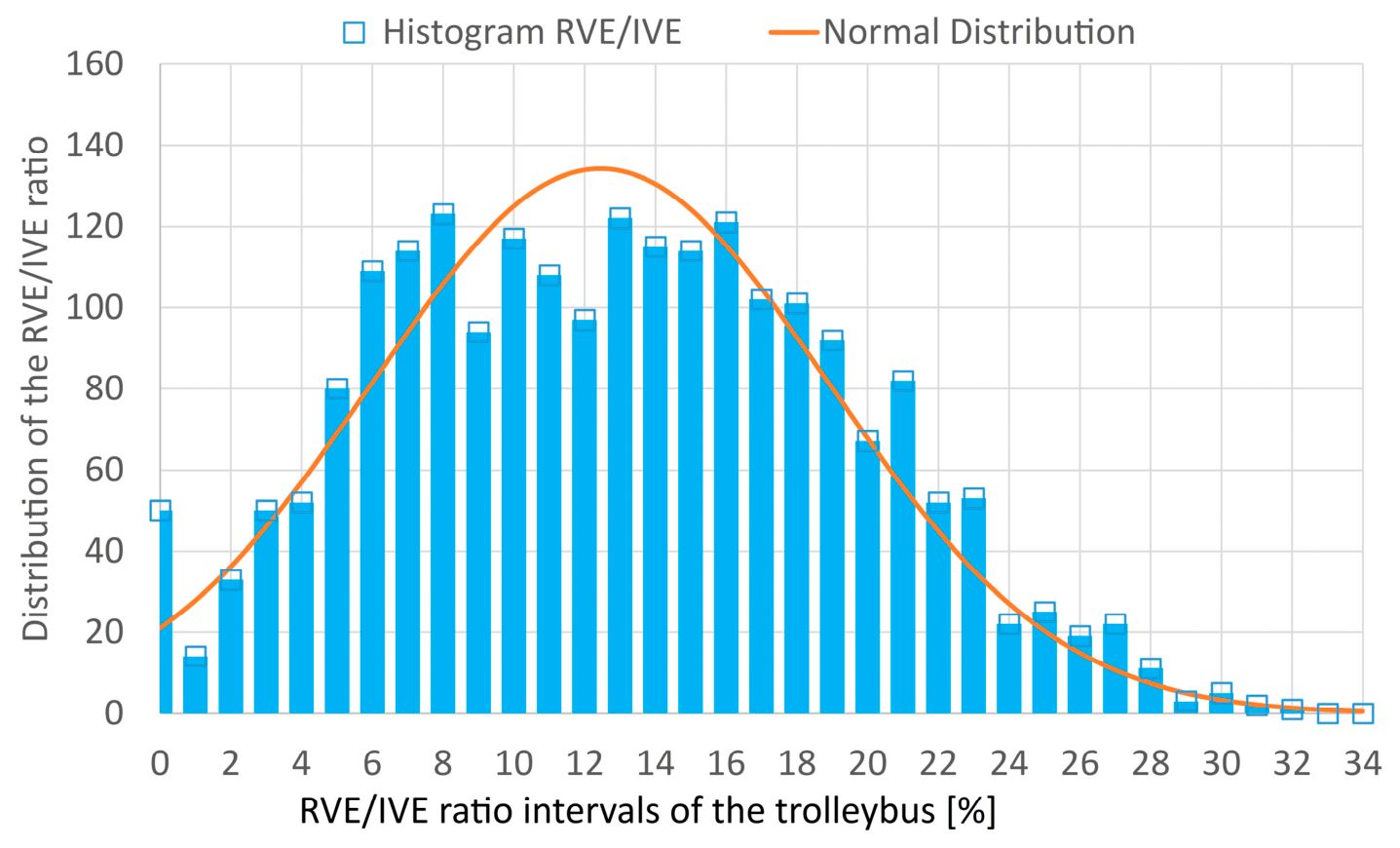
• Ratio of the energy regenerated into the catenary (Regeneration Vehicle Energy—RVE) and energy drawn from the catenary (Input Vehicle Energy—IVE)—Histogram RVE/IVE [%]—Figure 3;
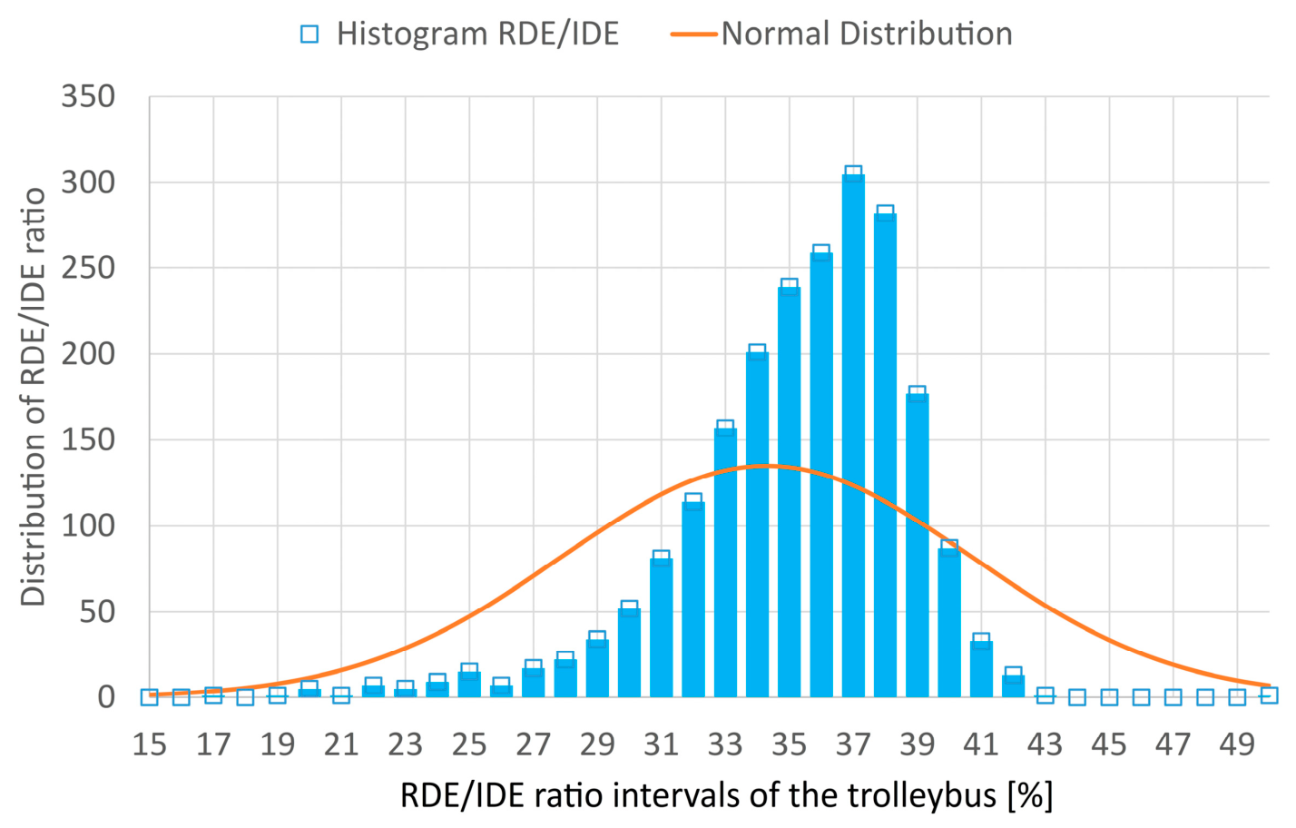
• Ratio of the regenerative braking energy (Regeneration Drive Energy—RDE) and energy drawn by the vehicle drivetrain (Input Drive Energy—IDE)—Histogram RDE/IDE [%]—Figure 4.

The appropriate class intervals are marked on the horizontal axis of the histograms, while the vertical axis shows the frequency of occurrence in the data analysis period for each class interval, i.e., 1 January 2016–30 June 2023.

The empirical distribution of the distance travelled by a trolleybus during one day of operation (Figure 1) shows that most often (about 230 times), the trolleybus covered a daily distance between 220 and 230 km. Frequent cases (over 200 times) are included in the class ranges 190–200, 210–220 and 240–250 km. The empirical distribution of the distance covered by a trolleybus powered only by a traction battery during one day of operation (Figure 2) shows that most often (about 550 cases), the trolleybus travelled a daily distance between 0 and 5 km. Frequent cases (over 200 times) are in the class range of 45–50 km. It is worth noting the distribution of this distance (about 100 cases) in a fairly wide class range of 10–35 km. About 50 cases were recorded for the class range above 80 km.

The empirical distribution of the relative value of energy regenerated into the catenary by a trolleybus per day (Figure 3) shows that most often (250 to 300 cases), the RVE/IVE parameter ranged from 5% to 17.5%. It should be noted that the empirical distribution for these class intervals was roughly uniform. The highest relative value of energy regenerated into the catenary was approximately 30%, but these were rare cases.

The empirical distribution of the relative value of regenerative braking energy per day (Figure 4) shows that most often (over 550 cases), the RDE/IDE parameter was in the range of 35% to 37%. This should be considered a good result, indicating relatively good efficiency of dynamic braking energy recuperation. It can be assumed that practically the entire distribution is concentrated in the 29–41% class range.

It can be assumed that the histograms presented in Figure 1, Figure 2, Figure 3 and Figure 4 represent a sample-based approximation of the probability distribution of a random variable. Since the number of samples is very high and the bins (intervals) are properly chosen (the Freedman–Diaconis rule), the histogram can closely resemble the true distribution. The essential parameters of random variables from Figure 1, Figure 2, Figure 3 and Figure 4 are given in

Table 1. Selected parameters of the distribution of random variables from Figure 1, Figure 2, Figure 3 and Figure 4.

Parameter	Figure 1	Figure 2	Figure 3	Figure 4
Expected value	188.91	28.69	12.45	34.28
Variance	5077.76	731.41	41.67	41.27
Standard deviation	71.26	27.04	6.455	6.42
Skewness	−1.162	2.6141	0.1682	−0.835
Kurtosis	66.13	20.26	−0.596	31.89

.

Additionally, Figure 1, Figure 2, Figure 3 and Figure 4 plot the normal distribution of the random variable at the same mean value and standard deviation as the empirical distribution. The purpose of this task was not to find the best approximation from known discrete or continuous theoretical distributions. The goal was to show how these empirical distributions differ from the normal distribution. The area under the histograms is equal to the area under the normal distribution.

The histogram parameters from Figure 1 indicate an average distance of approximately 189 km, and the measure of dispersion relative to the mean, i.e., equal variance, at approximately 5077 is relatively high. The standard deviation is about 71 km, so distances are quite spread out around the mean. The negative skewness of −1.16 means that the distribution has a longer tail on the left. There are more extreme low values than high values. The kurtosis of about 66 is relatively high, indicating very heavy tails and a strongly peaked centre.

The histogram parameters from Figure 2 indicate an average distance of approximately 28 km and a high variance value of about 731. The standard deviation of 27 km is greater than the mean value, so the spread is large relative to the mean. The distribution has a long right tail, so the skewness of 2.6 is positive and relatively high. Most distances in Battery mode operation are concentrated on the lower side, with some large values stretching the tail to the right. The kurtosis of about 20 indicates a high probability of extreme values—a very heavy tail and a sharp central peak.

The histogram parameters from Figure 3 indicate an average RVE/IVE ratio of about 12.45%, and variance of about 41 is moderate relative to the mean value. The standard deviation of approximately 6.4% indicates moderate dispersion around the mean value. The skewness of about 0.16 indicates a symmetric distribution with a tiny tilt to the right. Kurtosis has a relatively low negative value of −0.59 (excess kurtosis) and indicates a flatter peak than the normal distribution.

The histogram parameters from Figure 4 indicate an average RDE/IDE ratio of about 34.3%. The standard deviation of 6.42% relative to the mean value suggests moderate spread. The negative skewness of −0.83 is meaningful and indicates moderate negative (left) skew. The left tail of the distribution is longer. The kurtosis equal to 31.89 is extremely high (normal distribution has kurtosis equal to 3.0). It indicates very heavy tails and a very sharp peak.

3. Selected Waveforms and Analysis Criteria

3.1. Selected Waveforms—Daily Acquisition Dataset

The daily acquisition dataset is a set of data recorded within one 24 h period. It is convenient to show the waveforms for such a daily record, because all of the trolleybus operating states, especially Catenary mode and Battery mode, are visible to each other. In most daily datasets, there are several trolleybus operating states in Catenary mode and several in Battery mode. However, it should be noted that each daily trip is different even with the same trolleybus timetable.

The rated voltage and rated capacity of the battery are 613 V and 62 Ah, respectively. The battery disconnect voltage and charging voltage at 100% SOC controlled by the Battery Management System (BMS) are 420 V and 689 V, respectively.

The waveforms of selected variables presented in the figures in this chapter refer to the daily acquisition dataset from 1 July 2016 and have been grouped as follows:

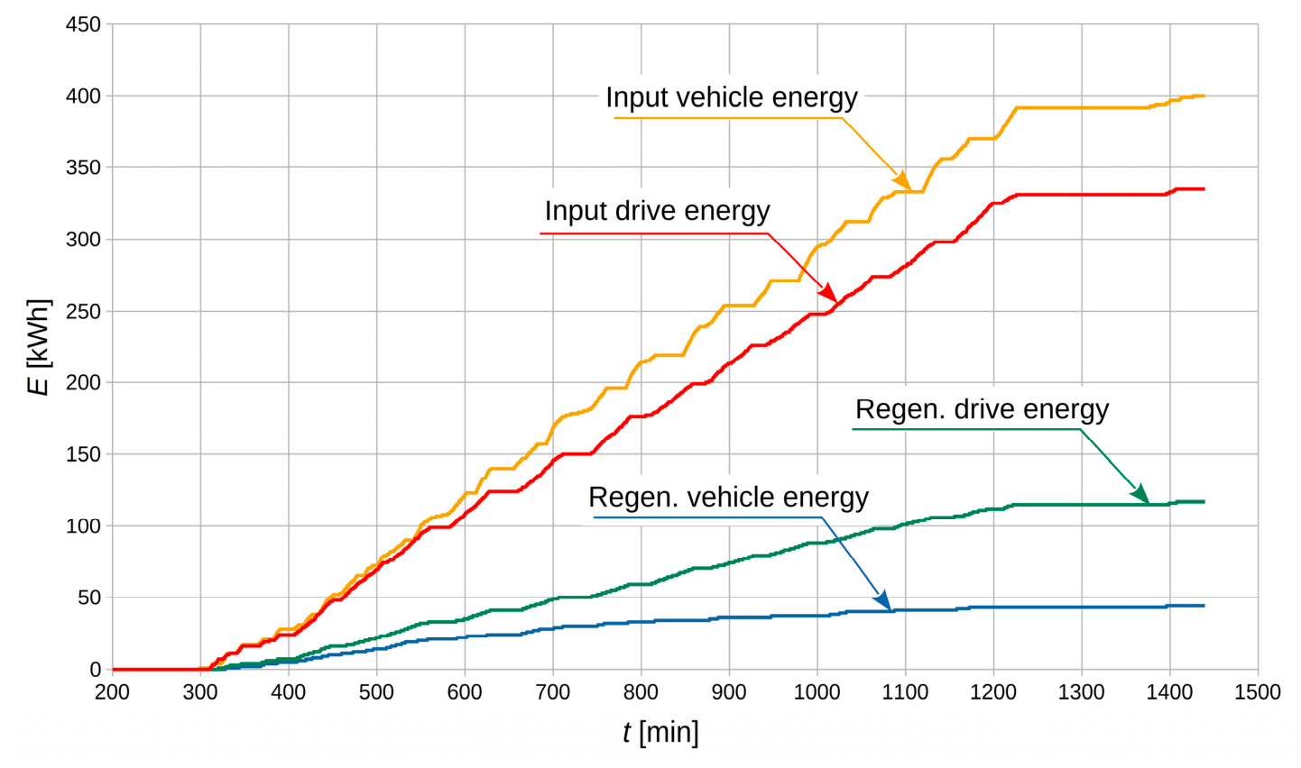
• Energy consumed by the vehicle from the catenary (Input vehicle energy), energy regenerated by the vehicle to the catenary (Regen. vehicle energy), energy consumed by the drivetrain (Input drive energy) and regenerative braking energy of the drivetrain (Regen. drive energy)—Figure 5.
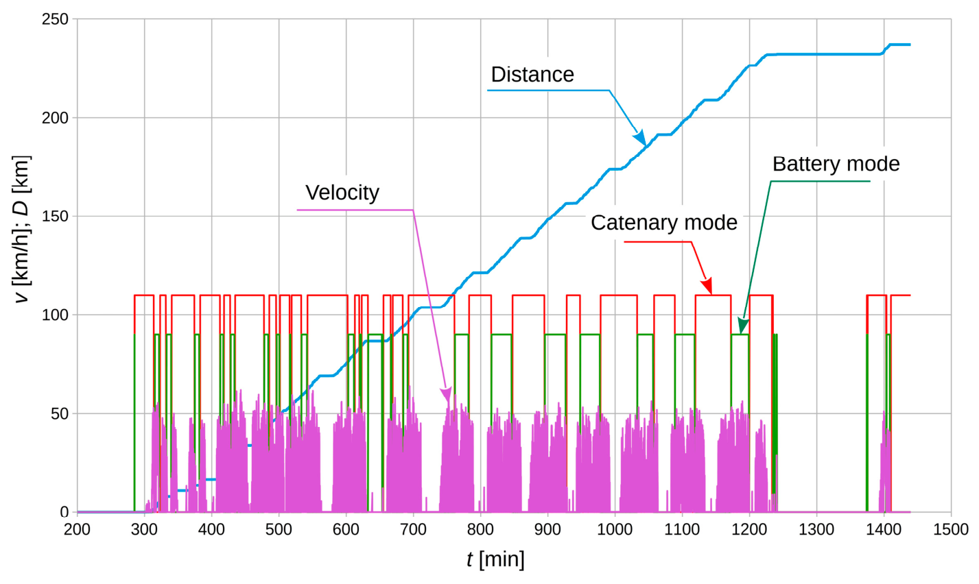
• Trolleybus operation mode—Catenary mode, Battery mode, distance covered and velocity. All those waveforms are shown in Figure 6. Battery mode and Catenary mode are binary values. In order to facilitate the distinction between trolleybus operating modes, Catenary mode–On has been assigned the value 110, while Battery mode–On has been assigned the value 90.
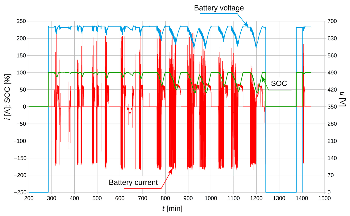
• Battery SOC status, battery voltage and current—Figure 7.

Comments and remarks about these waveforms are as follows:

• The vehicle covered a distance of 235 km, with a top speed of about 50 km/h.
• The energy consumed from the catenary was approximately 400 kWh, while 50 kWh was regenerated back into the grid. The ratio of recuperation was approximately 20%.
• The energy consumed by the drivetrain was approximately 330 kWh, while that of regenerative braking was approximately 120 kWh. The ratio of braking energy to energy consumed was approximately 36%.
• Operating modes—catenary power (Catenary mode) and battery power (Battery mode) generally alternate, but this is not a rule. There are several operating cycles in Battery mode and several in Catenary mode. The operating time intervals in Catenary mode are longer than those in Battery mode.
• When the drivetrain operates in Motoring mode, traction battery current (shown in Figure 7 as negative values) reaches a maximum value of 180 A, which translates to a discharge rate of 3C.
• Battery voltage decreases from about 670 V at 100% SOC to about 600 V when the SOC nears 50%.

The actual operating time in Battery mode depends on a number of factors, such as the number of passengers (trolleybus load), external temperature, battery temperature, road inclination, terrain profile, speed and even tire pressure [16].

3.2. Data Analysis Criteria Adopted for Assessing the SOH of the Traction Battery

There exist multiple methods for traction battery condition estimation [17,18]. Optimal operation of the traction battery ensured by the BMS is usually predictive and based on the measurement of the battery SOC [19,20]. In this paper, estimation of the battery condition was carried out solely on the basis of an analysis of long-term data recorded every day of trolleybus operation—historical data. The authors had no access to SOH examination results conducted with dedicated lithium-ion battery testers.

Battery charging process dynamics are dependent on the actual state of its capacity. Therefore, the authors decided to analyse in detail operation states in Catenary mode. In this mode, the battery is recharged from the catenary in accordance with the algorithm embedded in the BMS. It was assumed that the dynamics of the battery charge state depended on the degree of battery capacity loss.

In this study, two criteria for data analysis were adopted for the purpose of assessing its technical condition when the trolleybus is operating in Catenary mode:

• SOC criterion: SOC ∈ <SOC₁, SOC₂>,
• Voltage criterion: U_batt ∈ <U_batt1, U_batt2>.

In both cases, the values of the electrical charge and energy fed into the battery during charging in Catenary mode are analysed. During the process, no energy from the battery is consumed by the drivetrain.

In the SOC criterion, the charge and energy supplied to the battery are determined only within the SOC range between the arbitrarily assumed values SOC₁ and SOC₂.

In the voltage criterion, the charge and energy supplied to the battery are determined only within the battery voltage range U_batt between the arbitrarily assumed values U_batt1 and U_batt2.

The larger the ranges of the values <SOC₁, SOC₂> and <U_batt1, U_batt2>, the lower the uncertainty in determining the charge and energy supplied to the battery. When analysing historical data, however, care should be taken to ensure that as many cases as possible meet the criteria throughout the entire data acquisition period. The condition of the largest number of cases is not always met throughout the entire analysis period, which leads to a certain compromise.

After conducting the analysis, it was ascertained that the ranges:

• SOC ∈ <SOC₁ = 70%, SOC₂ = 100%>,
• U_batt ∈ <U_batt1 = 650 V, U_batt2 = 680 V>,

guarantee sufficient compromise to achieve relatively low uncertainty in the load and energy supplied to the battery and a relatively large number of these cases over the entire timespan covering the years 2016–2023.

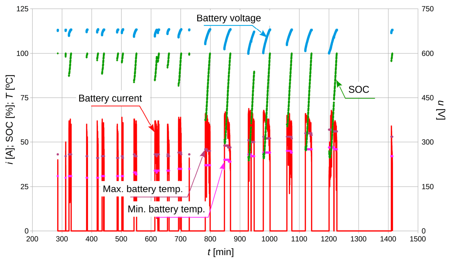
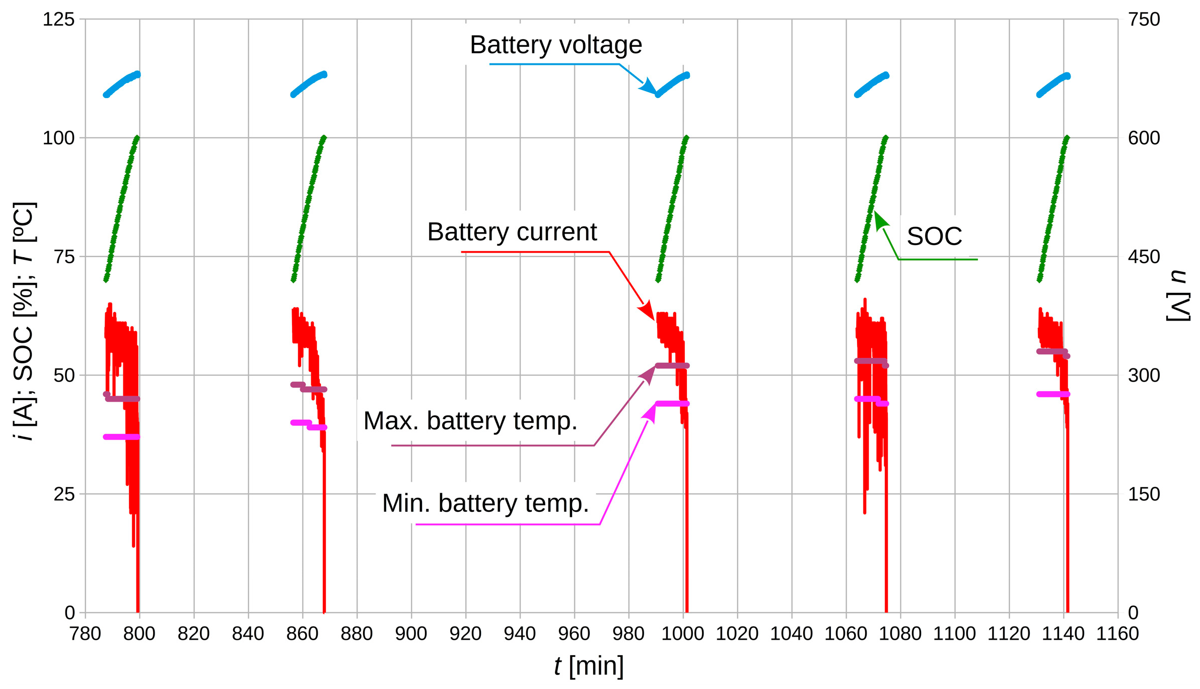
The algorithm for analysing the battery charging process in Catenary mode searches the database for all states of this process first. These states are shown in Figure 8, which include battery current and voltage, the SOC parameter, and minimum and maximum battery temperature. The manner of interpretation of minimum and maximum battery temperature should be explained here. The data acquisition system records only the minimum and maximum battery temperature values. It should therefore be assumed that some (perhaps most) of the battery cells operate at temperatures between these extreme values.

Analysis of the waveforms shown in Figure 8 shows that the battery charging process starts at different values: SOC, battery voltage, and minimum and maximum battery temperature. Therefore, the charging times required to reach a specific SOC level, which in the tested case was 100%, vary. The number of battery charging states for the acquisition package from 1 July 2016 is 20.

The next step is to implement the SOC or voltage criterion. This means that from the set of battery charging states shown in Figure 8, only those fulfilling the assumed criterion are selected.

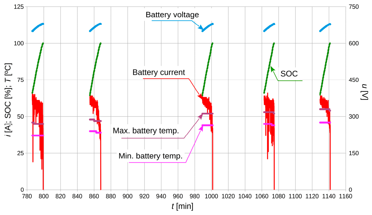
In Figure 9, the battery charging states with the applied criterion SOC ∈ <SOC₁ = 70%, SOC₂ = 100%> are shown, while in Figure 10, battery charging states with applied voltage criterion U_batt ∈ <U_batt1 = 650 V, U_batt2 = 680 V> are presented.

The algorithm found 5 cases fulfilling the SOC criterion and 4 cases fulfilling the voltage criterion. Consequently, daily collections of the data fulfilling given criteria were created. The sample size of such a daily collection within the analysed timespan 30 June 2013–1 January 2016 ranges between a few to over a dozen. The temperature range between the minimum and maximum values is (unfortunately) not equal when both the criteria are met. The temperature difference shown in Figure 9 is about 10 °C.

4. Charge and Energy Supplied to the Battery in Catenary Mode

Electrical charge Q and energy W supplied to the battery in the analysed trolleybus operation mode have been determined for each data collection fulfilling both the voltage and SOC criteria. For this task, numerical integration of the discrete data for each of the collection elements was carried out according to the following equations:

$$Q(k)={\displaystyle \underset{t_{1\left(k\right)}}{\overset{t_2\left(k\right)}{\int }}}{I}_{\mathrm{b}\mathrm{a}\mathrm{t}\mathrm{t}}\left(k\right)dt$$

(1)

$$W(k)={\displaystyle \underset{t_1\left(k\right)}{\overset{t_2\left(k\right)}{\int }}}{I}_{\mathrm{b}\mathrm{a}\mathrm{t}\mathrm{t}}\left(k\right)U_{\mathrm{b}\mathrm{a}\mathrm{t}\mathrm{t}}\left(k\right)dt$$

(2)

where I_batt(k), U_batt(k) are, respectively, the current and voltage arrays in the k-th collection, and t₁(k), t₂(k) are, respectively, the start time and end time of the charging process in the k-th data collection.

After determining the values of Q and W in the daily collection, the calculation algorithm moves on to the next daily collection (next iteration) in the trolleybus database and repeats the calculations according to Equations (1) and (2). The algorithm performs thousands of iterations until all daily datasets have been processed.

4.1. Charge and Energy of the SOC Criterion—Historical Data Span

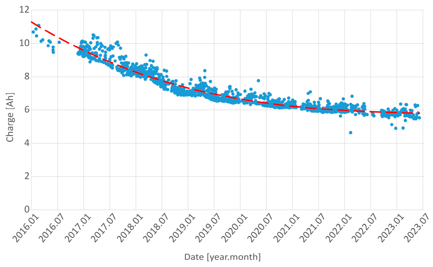
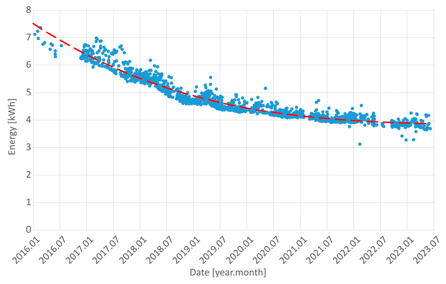
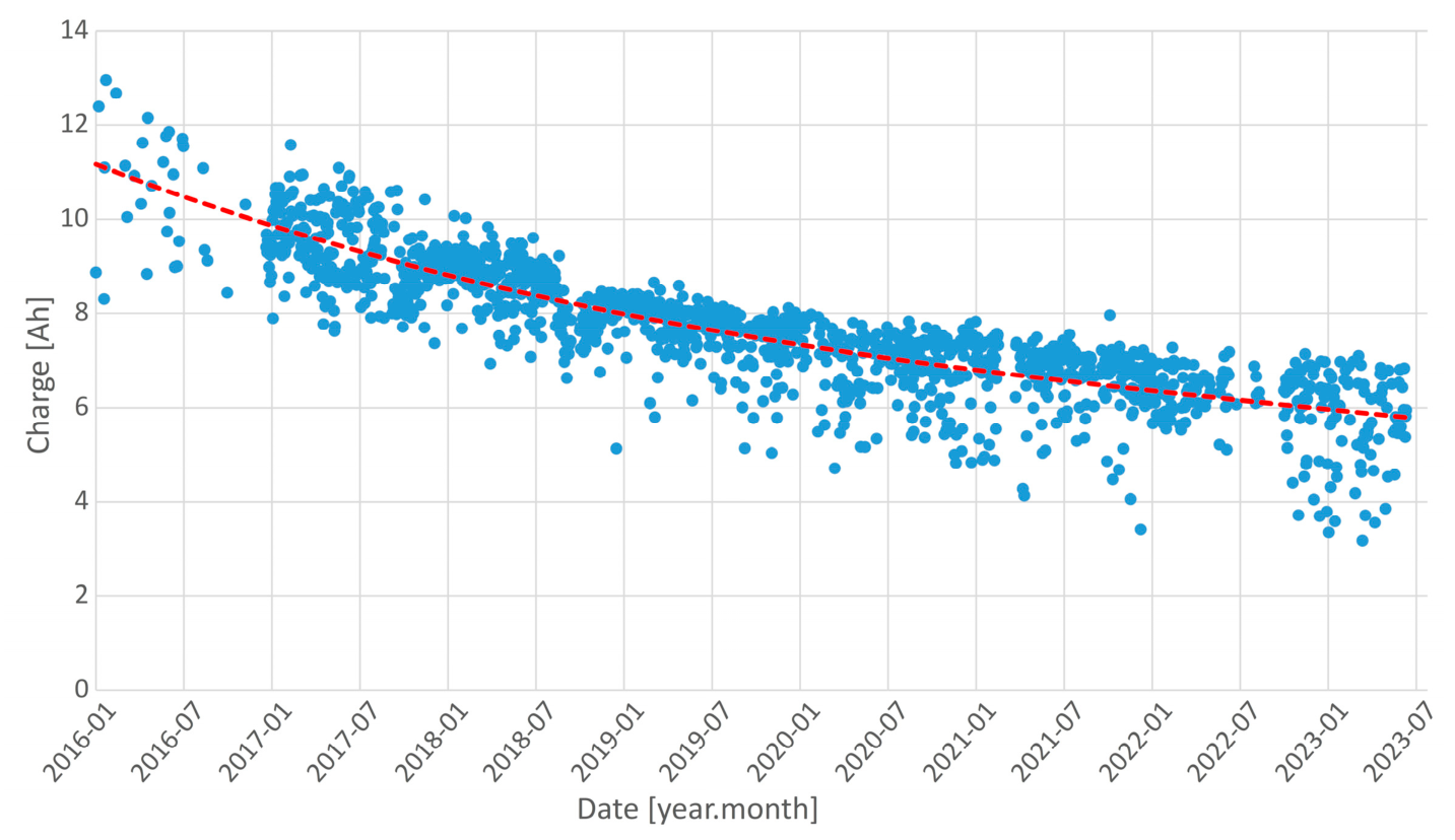
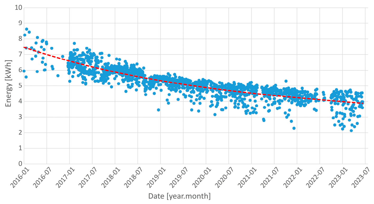
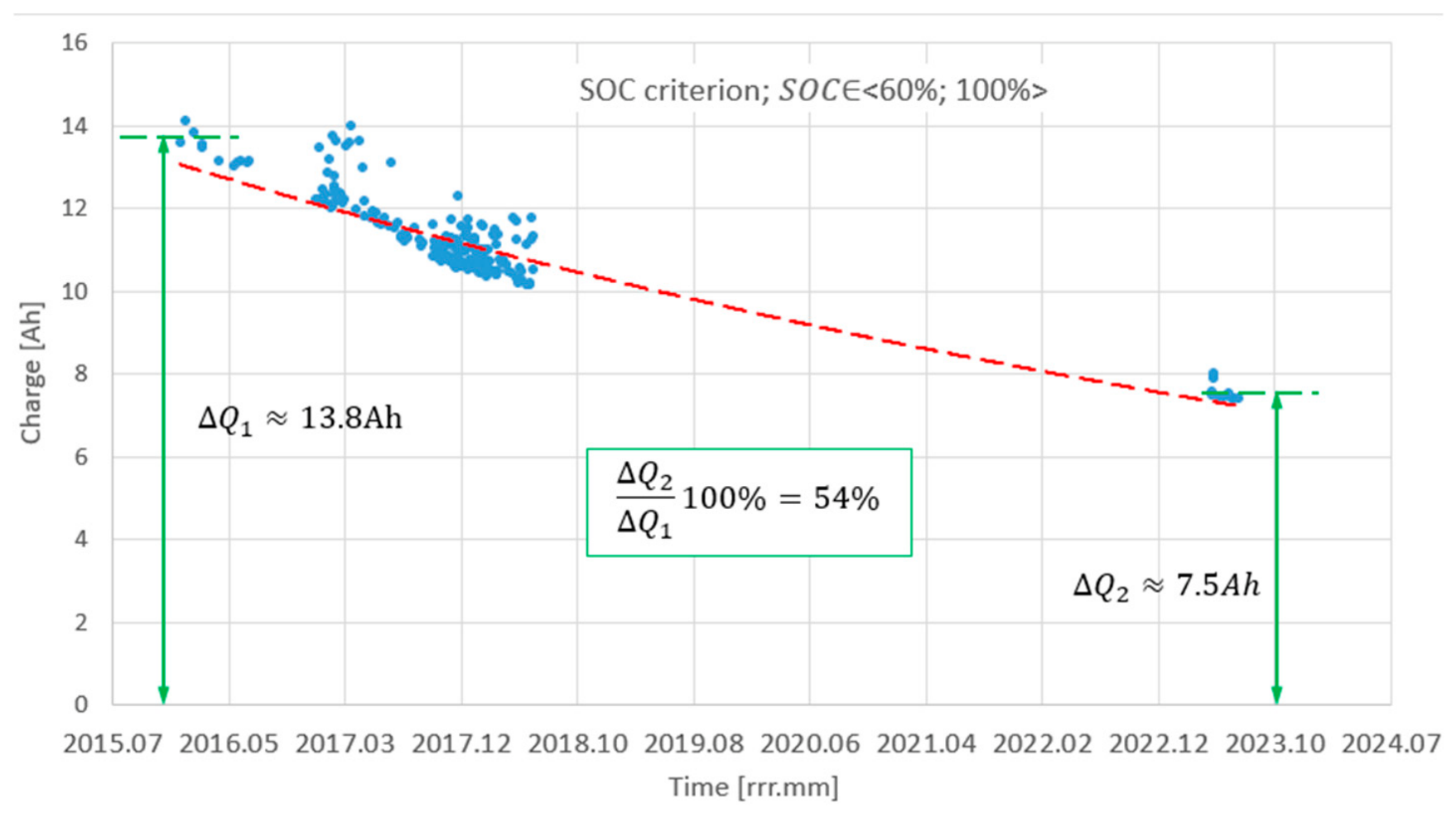
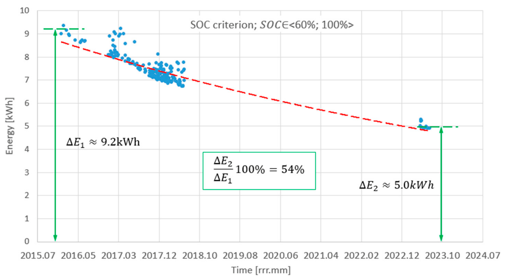
Results of the charge supplied to the battery are shown in Figure 11, and supplied energy in Figure 12. Those analyses apply to the criterion SOC ∈ <SOC₁ = 70%, SOC₂ = 100%>.

Both the charge and energy supplied to the traction battery decrease as a function of operation time. Such a result is expected, as it stems from the battery ageing process. Such conclusions have been reported in many research papers. However, the dynamics of these changes are important, as they depend on multiple factors and can differ between laboratory tests (controlled parameters) and tests carried out under vehicle operating conditions. In the first years of operation, the dynamics of changes of supplied charge and energy are the greatest. After six and a half years, the dynamics of these changes decrease and are relatively small, which is a good prospect for the SOH extrapolation into the future.

The results are relatively well centred around the trend line, defined by the 3rd order polynomial. Coefficients of these polynomials are shown in the respective graphs. In the first half-year of the vehicle operation (2016), there are fewer data collections fulfilling the assumed criteria. This is a consequence of conducting trial runs after the vehicle was delivered to the operator. The few data points deviating from the trend line result from the small size of some data collections meeting the assumed criteria, and, additionally, from significant differences between the minimum and maximum battery temperatures in the recorded daily datasets.

4.2. Charge and Energy of the Voltage Criterion—Historical Data Span

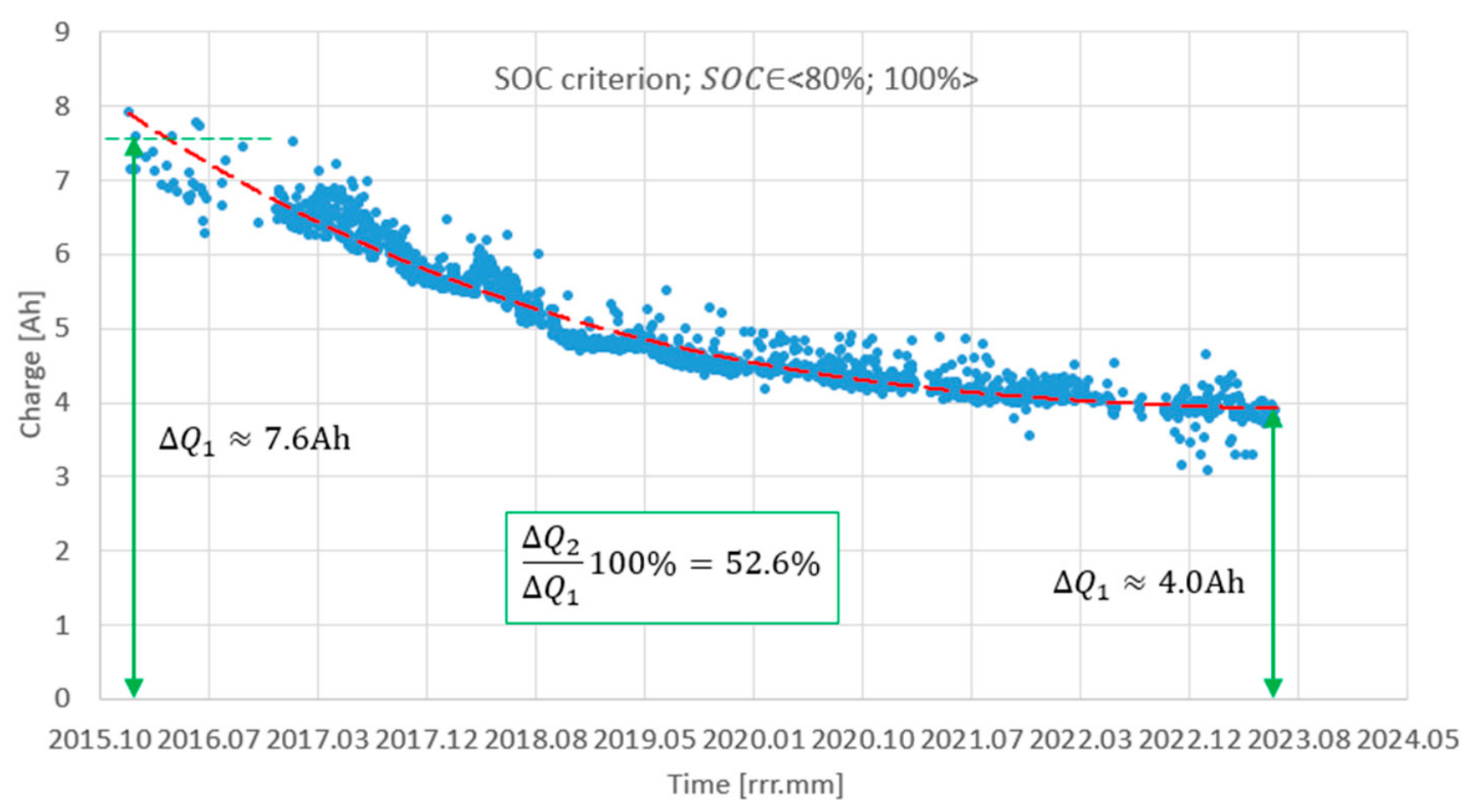
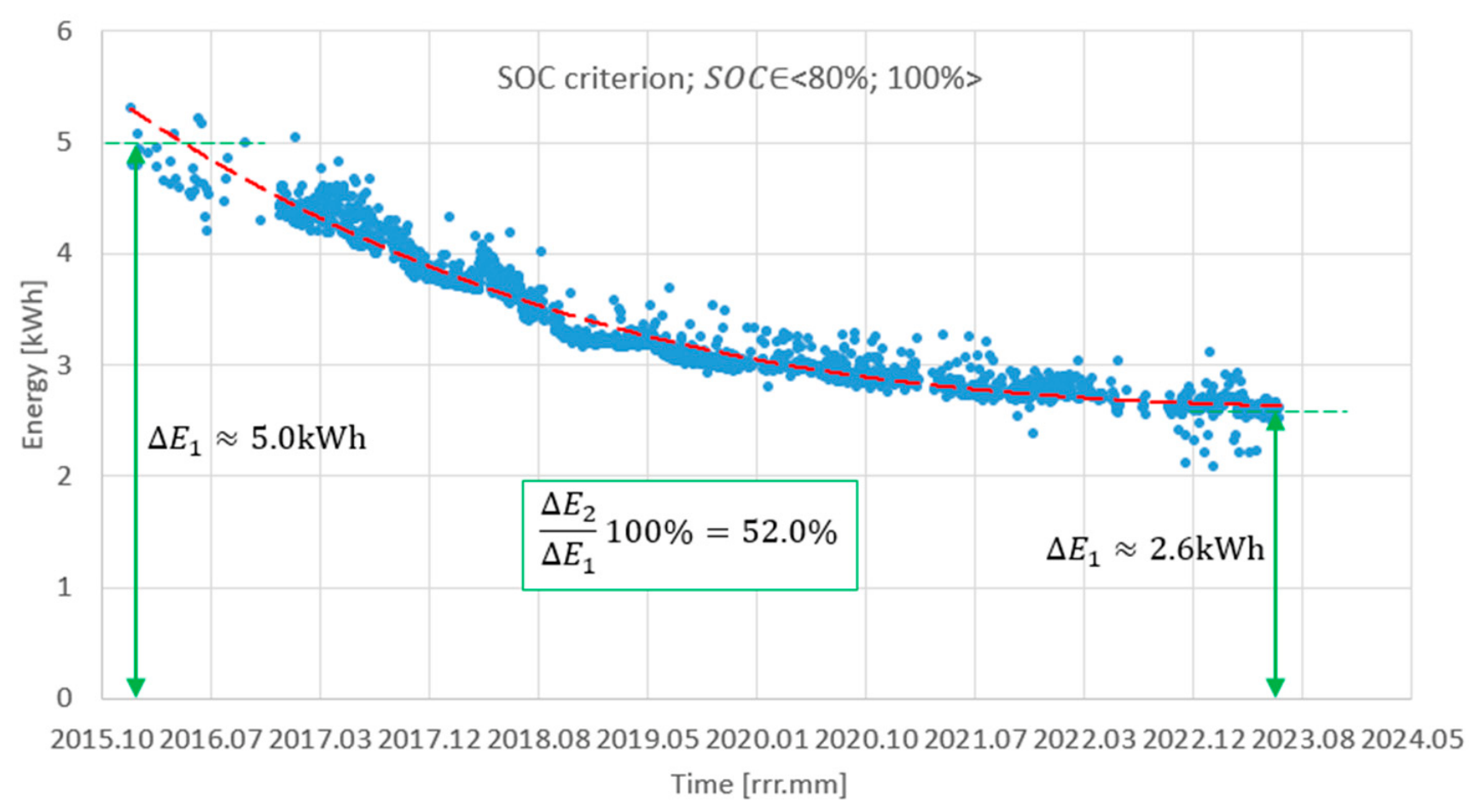
Results of the charge supplied to the battery are shown in Figure 13, and supplied energy in Figure 14. Those analyses apply to the criterion U_batt ∈ <U_batt1 = 650 V, U_batt2 = 680 V>.

Under this criterion, the charge and energy supplied to the traction battery expectedly decrease as a function of operation time—this is a consequence of the battery ageing. As stated before, the dynamics of these changes are important for the operator of the vehicle. The dynamics of the changes are the greatest in the first years of operation. After six and a half years of operation, the changes are less prominent.

Most of the results are relatively well centred around the trend line (3rd order polynomial); however, the deviation of some of the data points is higher for the voltage criterion than in the case of the SOC criterion. Coefficients of these approximating polynomials are shown in the respective graphs. Because of the trial operation in the first half-year of the vehicle service, there are fewer data collections that fulfil the voltage criterion.

In the first half of the vehicle’s operation (2016), a smaller number of data collections meeting the voltage criterion was observed, which results from a number of test drives of the tested trolleybus.

Analysis of the historical data shows that relatively good prediction of the battery SOH for the next year is possible if the trolleybus will be operated in atmospheric conditions and under a timetable similar to the ones from previous years.

Results shown in Figure 11, Figure 12, Figure 13 and Figure 14 do not take into account the battery temperature criterion. Consequently, some of the results are further from the trend line, as the impact of the battery temperature on SOH is significant. The preferred range of the operational temperature for lithium-ion cells lies between 25 °C and 40 °C, according to the manufacturer data [21,22]. Analysis of the historical data revealed that the maximum temperature exceeds 40 °C. However, this value does not indicate that such a temperature occurs in all the cells of the battery, as mentioned earlier. An accurate value of the temperature of the cells is of key importance for the BMS system, as it could prevent overheating of the battery [23].

5. Factors Influencing Degradation of Lithium-Ion Batteries

5.1. Mechanisms of Battery Degradation

The ageing process of a battery over a long period of operation stems from two fundamental degradation mechanisms [24,25,26]: calendar ageing and cycling ageing. Calendar ageing occurs when the battery does not absorb or release energy to an external electrical circuit. Research presented in [27] indicates that calendar ageing of a battery stored for 5 years at 25 °C reduces its capacity to 90%, while at 45 °C, capacity drops to 75%. The SOC value affects battery capacity loss as well. Research results presented in [28] indicate a 25% capacity loss when the battery is stored at SOC = 100% for 9 years. Calendar ageing also affects the battery’s internal resistance—an increase of 15% at 45 °C after 3 years of storage [29].

Cycling ageing occurs when the battery is being charged or discharged and depends on many factors, including the frequency of charge and discharge cycles. A number of factors contribute to the degradation of lithium-ion batteries during their service life (cycling ageing). The main factors in this regard include [30]:

• Battery cell temperature [31,32,33,34].
• Discharging current value [35,36,37,38].
• Charging current value [38,39,40,41].
• SOC or DOD level [38,42,43].

The factors listed above have varying effects on the degradation of the basic components of the battery (electrodes, electrolyte, separator, etc.).

The factors influencing the anode area/domain degradation are as follows:

• High SOC—effect: Formation of a layer of metallic lithium (lithium plating) [44], leading to reduced capacity and internal short circuits; electrolyte decomposition into undesirable by-products [45,46].
• Low SOC—effect: Anode corrosion [47]; Electrolyte decomposition [45].
• High temperature [27,44,48]—effect: Gradual increase in the thickness of the solid electrolyte interphase (SEI) layer; Phase change in the anode’s active material caused by metal dissolution.
• Low temperature [44,49]—effect: Metallic lithium platting on the anode during charging.
• High current rate [44,50,51]—effect: Deposition of metallic lithium and degradation of the electrolyte; Thickening of the solid electrolyte interphase (SEI) layer; Loss of active material particles (LAM).

Key factors influencing the cathode area/domain degradation are as follows:

• High SOC—effect: Corrosion of the cathode [47]; Electrolyte decomposition [46].
• Low SOC [46]—effect: Cathode corrosion; Flushing metal ions (Mn, Ni, Co) from the cathode structure towards the anode (transition metal dissolution); Electrolyte decomposition.
• High temperature [27,28,50]—effect: Degradation of the cathode crystal structure due to increase in phase changes in the active material; Loss of recyclable lithium within the battery.
• High current load [44,45,50]—effect: Flushing of metals (Mn, Ni, Co) from the cathode structure, which migrate towards the anode (transition metal dissolution); Mechanical breakdown (particle cracking) of the cathode’s active material (active material crumbling).

5.2. Impact of the SOC on Battery Degradation

The maximum value of the SOC recorded in the analysed trolleybus was 100% at the end of each charging process. This is not a condition recommended by manufacturers of Li-ion batteries, especially NMC batteries. The recommended maximum SOC is typically 80%. Therefore, this factor may have had some impact on the degradation of the NMC batteries in the considered trolleybuses. However, it should be noted that once the SOC reached 100%, the trolleybus immediately switched to Battery mode, which caused the SOC value to drop. The SOC = 100% state during public transport service was always very brief. At the depot, however, the battery remained at a SOC close to 100% for several hours. Considering this 6 h idle state of the battery at SOC = 100% and assuming only calendar ageing, the loss of initial capacity is approximately 8% over six and a half years of operation, according to the characteristics given in [28]. This is, therefore, not the primary factor in degradation, but it should be taken into account.

The minimal SOC value in the analysed trolleybuses never fell below 30%, and values close to this threshold were rarely observed. Therefore, it could be ascertained that the low SOC factor did not play a role in degradation of the analysed batteries.

5.3. Impact of Temperature on the Degradation of the Analysed Battery

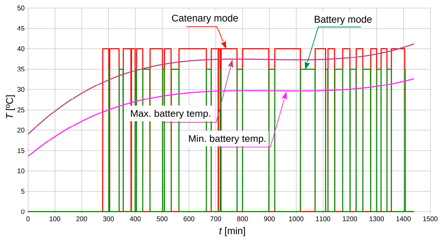
The maximum and minimum battery temperature waveforms were not uniform during a single day of a public transport service. When the vehicle began its service (departure from the depot), the temperature values were typically at their lowest. The temperature generally increased as the service progressed. The maximum and minimum temperature waveforms also varied across individual daily datasets. Figure 15 shows the maximum and minimum temperature profiles for the service on 14 June 2018, where the minimum outside temperature was approximately 13 °C and the maximum outside temperature was approximately 22 °C. Additionally, the vehicle operating states are shown as rectangles: Battery mode—battery operation mode, and Catenary mode—vehicle operation mode when powered from the catenary.

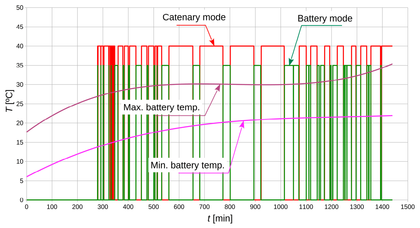
Figure 16 shows the maximum and minimum temperature curves for the service on 7 February 2018, where the minimum outdoor temperature was approximately −8 °C and the maximum outdoor temperature was approximately +0.5 °C.

The case shown in Figure 15 is representative of service provided during the summer months, while the case in Figure 16 is representative of service provided during the winter months.

Two key conclusions emerge from the analysis of these waveforms. First, the maximum and minimum temperature curves exhibit a monotonically increasing trend. Second, during operation in the winter months, the temperature curves have lower values than those under summer conditions.

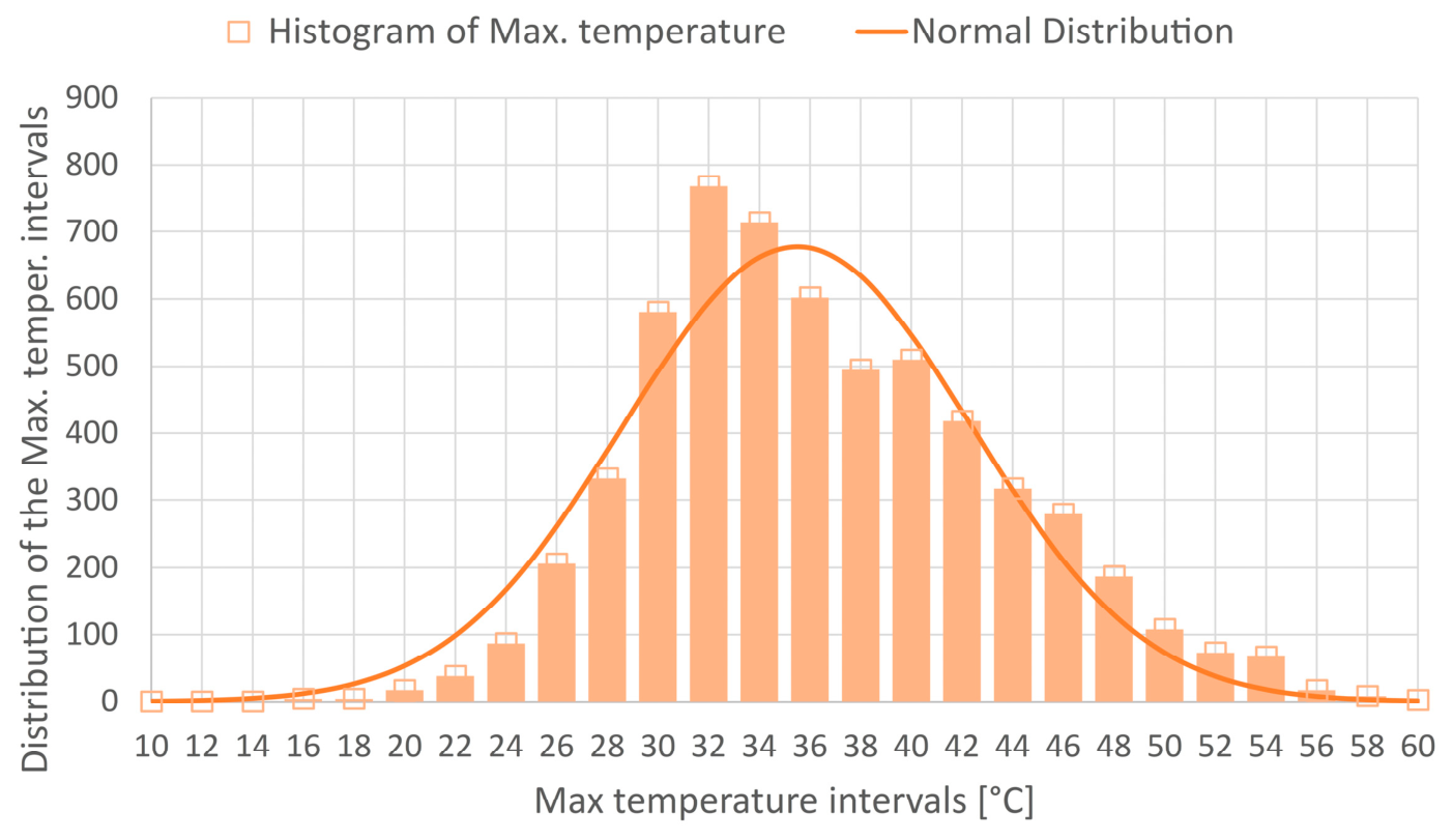
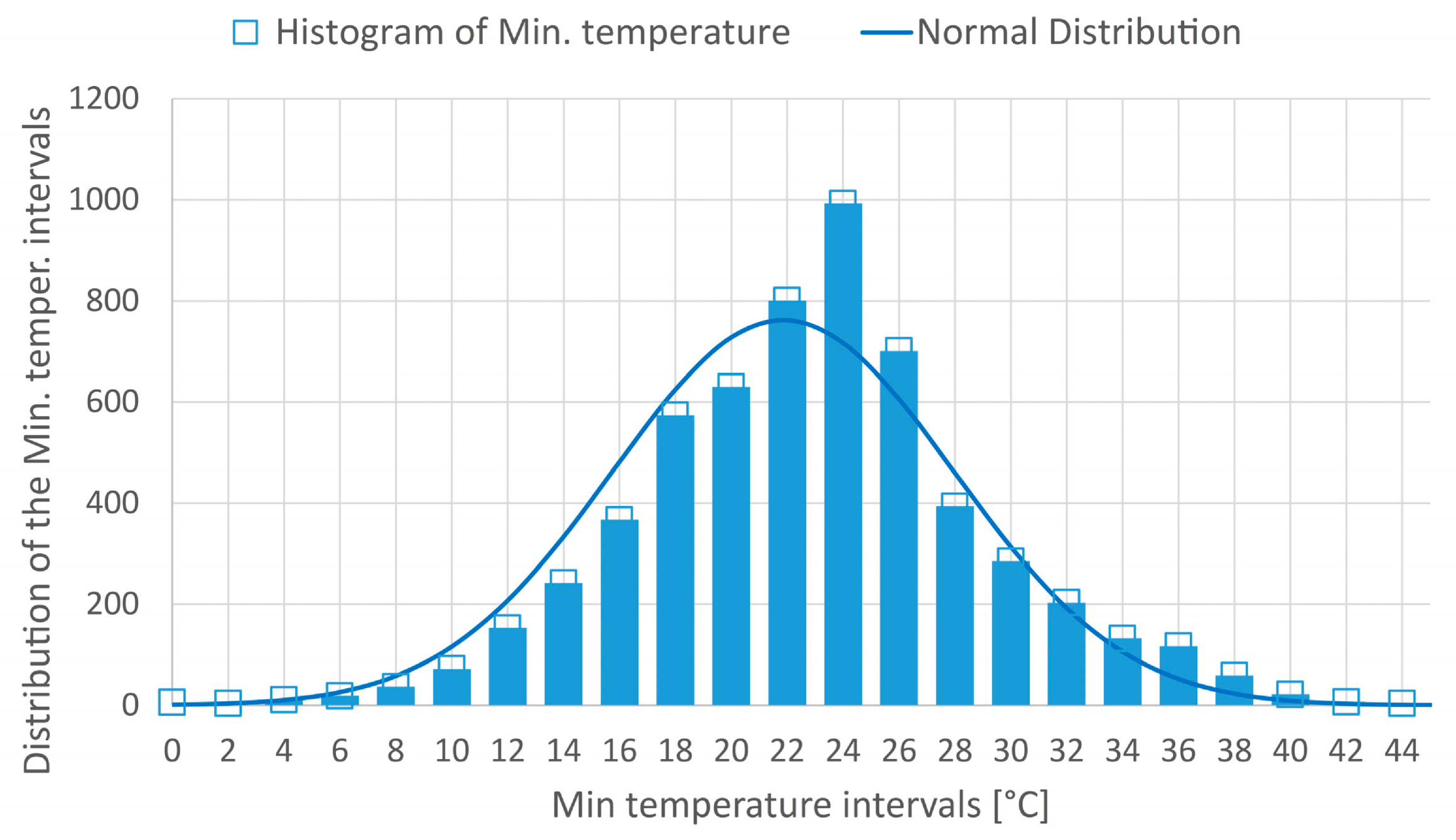
For the purpose of quantitatively assessing the impact of temperature on battery degradation, empirical distributions of minimum and maximum temperature values are presented, referenced to the criterion SOC ∈ <SOC₁ = 70%, SOC₂ = 100%> for the entire data analysis period, i.e., 1 January 2016–30 June 2023. The presented quantitative characteristics/distributions are as follows:

• Maximum battery temperature—Figure 17;
• Minimum battery temperature—Figure 18.

Numerical characteristics of selected random variables from Figure 17 and Figure 18 are given in

Table 2. Selected parameters of the empirical distribution of random variables from Figure 17 and Figure 18.

Parameter	Figure 17	Figure 18
Expected value [°C]	35.49	21.85
Variance [°C2]	47.2	37.3
Standard deviation [°C]	6.87	6.11
Skewness [-]	0.411	0.071
Kurtosis [-]	−0.14	0.53

.

The histogram parameters from Figure 17 indicate an average max temperature of about 35 °C. The standard deviation is about 6.8 °C, so it indicates moderate spread. The positive skewness of 0.411 is relatively small. It means that the right tail is slightly longer than the left. The kurtosis is very low, indicating that the distribution is very close to normal.

The histogram parameters from Figure 18 indicate an average min temperature of about 22 °C. The standard deviation is about 6.1 °C, indicating moderate spread. The positive skewness of 0.07 is very small. It means that the right tail is slightly longer than the left. The kurtosis is very low, indicating that the distribution is very close to normal.

The authors decided to determine the theoretical distribution of the random variable, which closely corresponds to the empirical distributions from the temperature histograms. Taking into account the numerical parameters from Table 2, the normal distribution seems to be a good solution. The probability density f₁(x) of the normal distribution approximating the histogram from Figure 17 is given by Formula (3). The probability density f₂(x) of the normal distribution approximating the histogram from Figure 18 is given by Formula (4). The expressions of the distributions f₁(x) and f₂(x) are as follows:

$$f_1\left(x\right)=K_n{\displaystyle \frac{1}{{\sigma }_1\sqrt{2\pi }}}{e}^{-{\displaystyle \frac{{\left(x-{\mu }_1\right)}^2}{2{\sigma }_1^2}}}$$

(3)

$$f_2\left(x\right)=K_n{\displaystyle \frac{1}{{\sigma }_2\sqrt{2\pi }}}{e}^{-{\displaystyle \frac{{\left(x-{\mu }_2\right)}^2}{2{\sigma }_2^2}}}$$

(4)

$$K_n=∆T·N$$

(5)

where ∆T = 2 °C is the width of temperature interval; N = 5834 is the number of empirical temperature samples; μ₁ = 35.49 and σ₁ = 6.87 are the mean and the standard deviation values of the maximum temperature histogram; μ₂ = 21.85 and σ₂ = 6.11 are the mean and the standard deviation values of the minimum temperature histogram.

It can be concluded that both empirical distributions are well approximated by normal distributions.

Based on the maximum temperature histogram, it can be concluded that within the temperature range of 29 °C to 35 °C, the class interval has the highest frequency, amounting to approximately 2200. The effect of maximum temperature on the parameters of the battery under test is twofold. First, studies presented in [32] have shown that the capacity of battery cells increases with rising temperature up to approximately 45 °C, which is a beneficial phenomenon—greater vehicle range. Above a temperature of approximately 45 °C, battery capacity decreases. On the other hand, unfortunately, the rate of battery degradation increases with rising temperature [32]. These are, therefore, opposing processes that require a compromise between achieving greater capacity and an acceptable rate of degradation. Comprehensive studies presented in [52] have shown that the maximum cycle count of a Li-ion battery is highest (approximately 2600 cycles) at a temperature of about 25 °C, with the battery’s capacity reduced to 80% of its initial value. At a temperature of 45 °C, the number of cycles decreased to approximately 1900. The histogram in Figure 17 shows that the frequency of class intervals above 45 °C decreases relatively quickly, but they contribute significantly to battery degradation.

The histogram of minimum temperatures shows that the largest number of data points falls within the temperature range of 16 °C to 26 °C. No sub-zero operating temperatures were recorded, and the number of data points above 30 °C is relatively small. Based on this, it can be concluded that the effect of minimum temperature on the rate of battery degradation is relatively small.

However, it should be noted that the recorded minimum and maximum temperatures are extreme values. It can be assumed that most battery cells operate between these extreme temperatures. This mitigates to some extent the effect of the maximum temperature on the degree of battery degradation. It would be advisable to collect data from a larger number of temperature sensors in the battery—not just the extreme ones.

5.4. Impact of Charging and Discharging Current on the Degradation of the Analysed Battery

The maximum battery charging current in the operation mode was around 60 A. Nominal battery capacity C = 62 Ah; therefore, the battery was charged at a rate of 1C. Under such conditions, it can be assumed that the End-of-Life (EOL) parameter of the Li-ion NMC battery is about 3000 charge/discharge cycles [53]. Charging and discharging currents impacts the battery SOH and RUL of the battery regardless of their values; however, at 1C current it can be assumed that it is not the main factor of battery degradation.

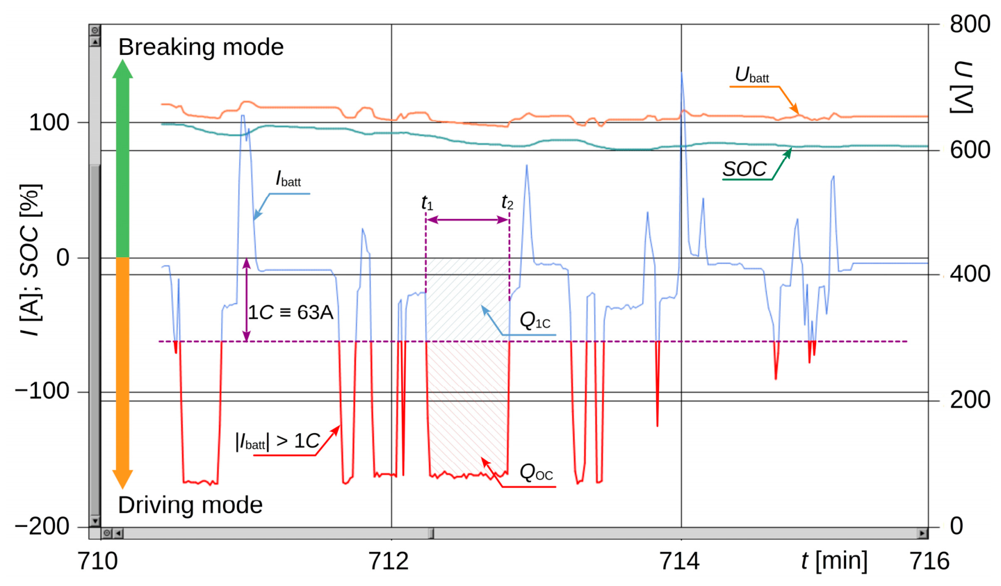
The maximum discharge current in Battery mode is significantly higher than the charging current in Catenary mode. The maximum discharge current is 180 A and is likely limited by the BMS. This means that the maximum discharge current was equivalent to 3C. This factor had a significant impact on the degradation of the tested battery. To approximate a quantitative assessment of the discharge current impact, the authors proposed an original approach, which will be discussed using the example of the current waveform in Battery mode shown in Figure 19. These are selected waveforms that can be considered representative of the battery operation in Battery mode. This figure shows two battery operating states: the state in which the trolleybus drive system is powered by the battery, where energy is drawn from the battery (Motoring mode), and the state in which the battery is charged during dynamic braking, where energy flows into the battery (Braking mode). In Motoring mode, the current values are negative, while in Braking mode, they are positive. In this figure, the battery current I_batt in Motoring mode is shown in two colours—blue and red. The red portion of the current waveform corresponds to an instantaneous value of I_batt(t) ≤ −63 A i.e., above 1C (in absolute terms).

Based on this defragmentation of the current waveform, two regions/areas can be defined, labelled in Figure 19 with the symbols Q_1C (current to 1C) and Q_OC (Over Current—current above 1C). The Q1C area represents the charge drawn from the battery during the time interval t ∈ <t₁, t₂> at a constant current value of I_batt = −63 A. The Q_OC field represents the charge drawn from the battery in the time window t ∈ <t₁, t₂>, but at a current of I_OC(t) = I_batt(t) − 63 A. In other words, Q_OC determines the portion of the charge drawn from the battery when the battery current exceeds 1C (in absolute terms). The values of these fields can be determined by numerically integrating the current with respect to time:

$$Q_{1\mathrm{C}}=\left|{\displaystyle \underset{t_1}{\overset{t_2}{\int }}}\left(I_{\mathrm{b}\mathrm{a}\mathrm{t}\mathrm{t}}=-63\right)dt\right|$$

(6)

$$Q_{\mathrm{O}\mathrm{C}}=\left|{\displaystyle \underset{t_1}{\overset{t_2}{\int }}}{I}_{\mathrm{b}\mathrm{a}\mathrm{t}\mathrm{t}}\left(t\right)dt\right|-Q_{1C}$$

(7)

The Q_1C and Q_OC areas are determined for every case where I_batt ≤ −63 A, with the exception of very short time intervals where the waveform contains only a few discrete current values and numerical integration would introduce significant errors.

Additionally, Figure 19 shows the battery voltage and SOC waveforms. These waveforms are only monotonic intervals, indicating dynamic changes in battery voltage and SOC when the system operates in Battery mode. The voltage and SOC waveforms of the battery are characterised by high dynamics of change. However, one can notice time intervals where the SOC or voltage curve is monotonic.

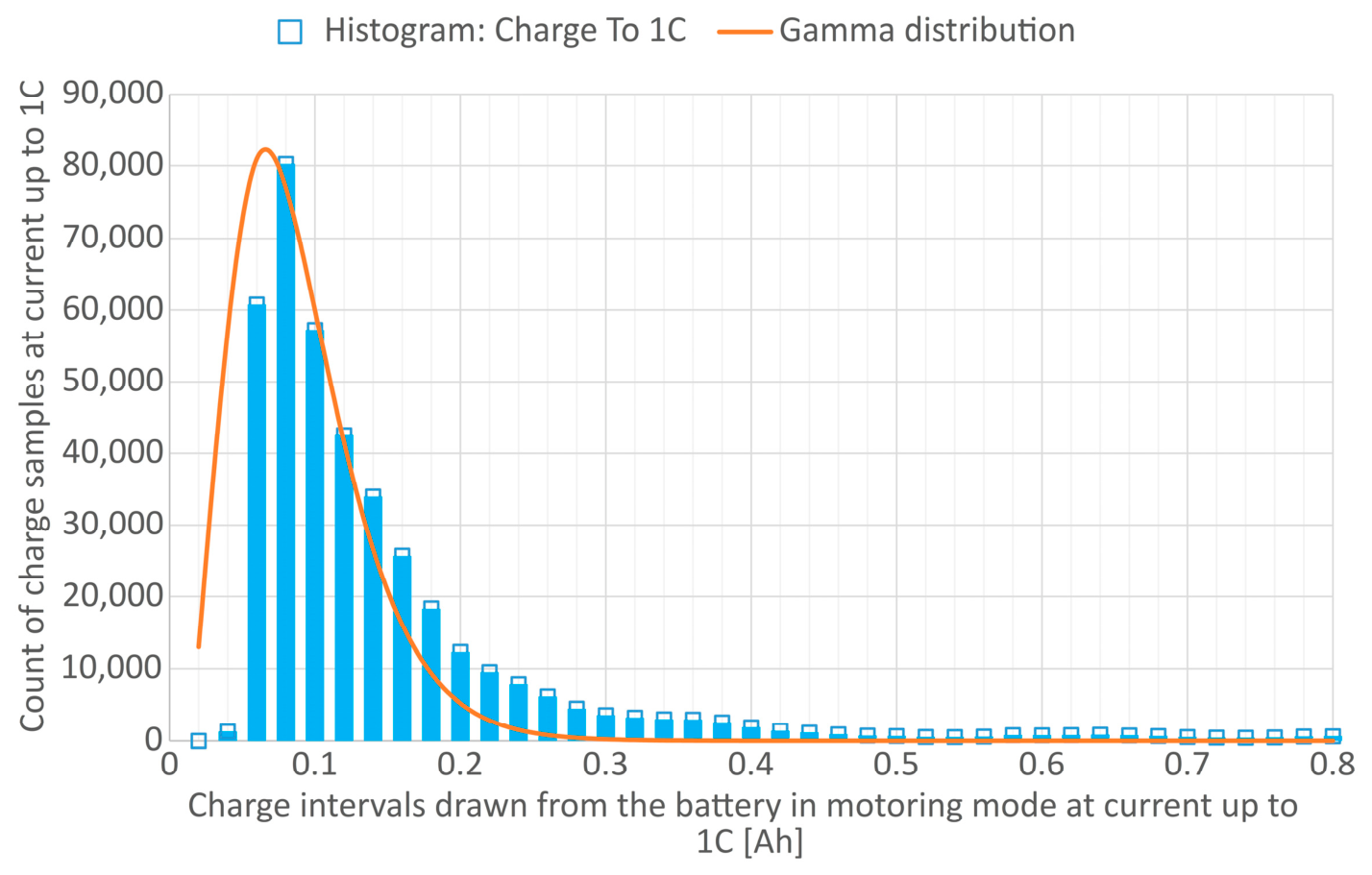
The next stage of the analysis involves generating histograms of the Q_1C and Q_OC charges, which are shown in Figure 20 and Figure 21, respectively.

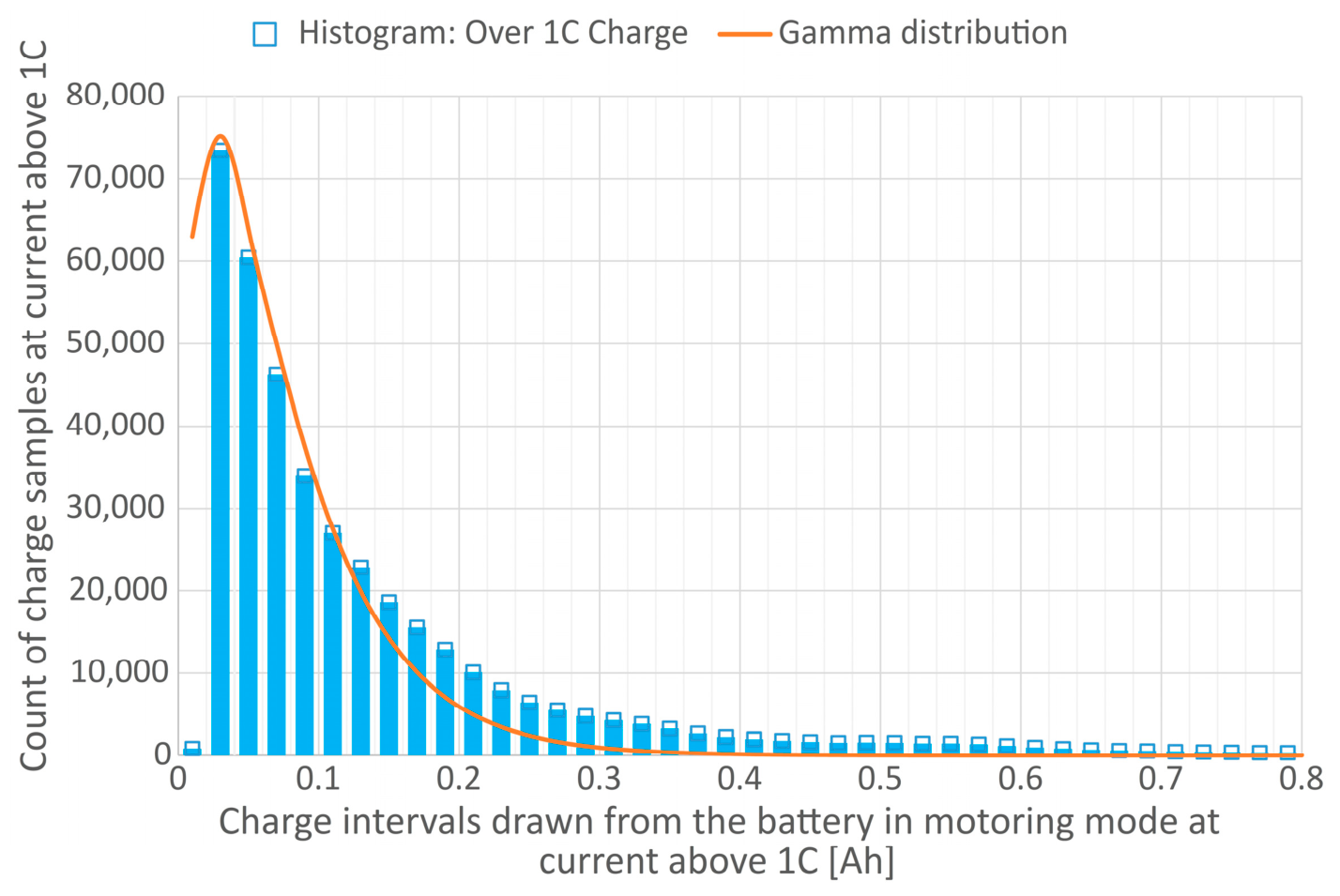
Analysis of the histogram in Figure 20 shows a maximum frequency in the class interval (over 80,000) for a discharged charge in the range of 0.04 to 0.06 Ah. The charge Q_1C drawn from the battery during discharge is relatively small compared to the battery rated capacity C_n = 63 Ah. However, these doses are very numerous, which is understandable given the battery’s six and a half years of operation.

Analysis of the histogram in Figure 21 shows a maximum class interval count (approximately 75,000) already at a Q_OC charge dose in the range of 0.0 to 0.02 Ah. Subsequent Q_OC charge doses have class interval frequencies that decrease monotonically. The Q_OC charge doses drawn from the battery are relatively small but also very numerous.

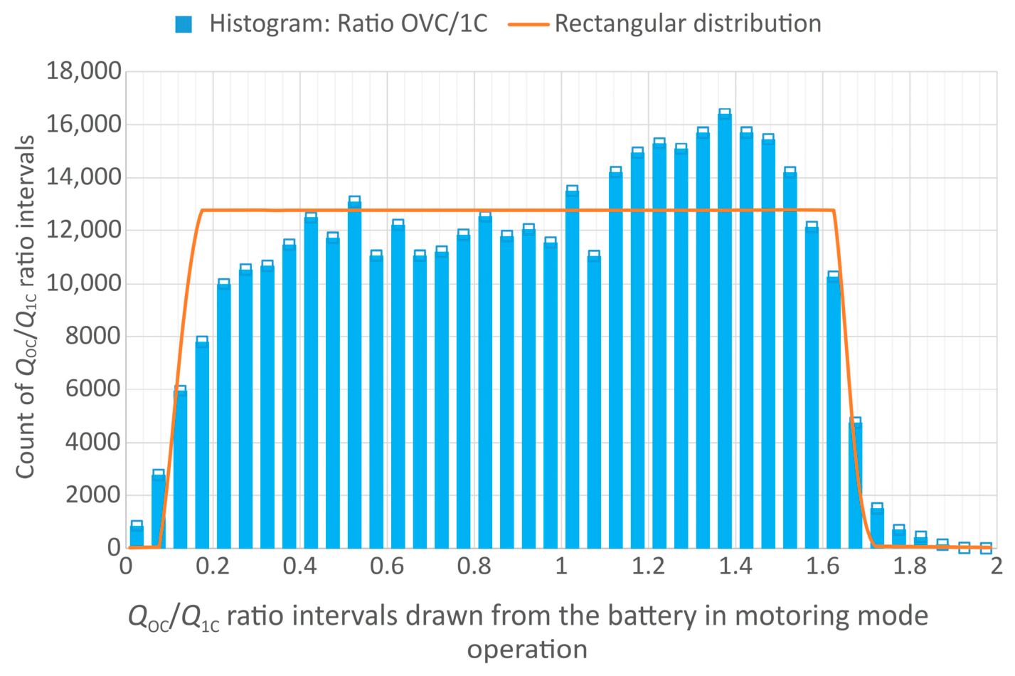
Comparing the charge doses Q_1C and Q_OC allows for an analysis of their ratio, i.e., Q_OC/Q_1C. This ratio does not exhibit any singularities, as the denominator is always greater than zero. Figure 22 shows a histogram of the Q_OC/Q_1C ratio for all Motoring mode battery operating states during the period 1 January 2016–30 June 2023. Analysis of the histogram in Figure 22 shows that the value of Q_OC/Q_1C in the range of 0.3 to 1.0 is characterised by a similar class interval count of approximately 12,000. For Q_OC/Q_1C values in the range of 1.1 to 1.5, the number of class intervals is the highest, exceeding 14,000. Unfortunately, this Q_OC/Q_1C range is the most critical in terms of battery degradation, which stems from the fact that the absolute value of the battery current |I_batt| is greater than 1C and the frequency of such states is the highest. The results of studies shown in [36] indicate that at discharge currents corresponding to 1C, 2C and 3C, a Li-ion battery loses 9.5%, 13.2% and 16.9% of its initial capacity, respectively, after just 350 charge–discharge cycles.

At Q_OC/Q_1C values above 1.6, the number of class intervals decreases significantly, which contributes to battery degradation, but to a lesser extent.

Numerical characteristics of selected random variables from Figure 20, Figure 21 and Figure 22 are given in

Table 3. Selected parameters of the empirical distribution of random variables from Figure 20, Figure 21 and Figure 22.

Parameter	Figure 20	Figure 21	Figure 22
Expected value	0.119 [Ah]	0.136 [Ah]	0.892 [-]
Variance	0.0159	0.0393	0.1984
Standard deviation	0.126 [Ah]	0.198 [Ah]	0.445
Skewness [-]	3.87	3.85	−0.155
Kurtosis [-]	29.65	27.9	−1.149

.

The authors decided to determine the theoretical distributions of the random variable, which closely corresponds to the empirical distributions from the histograms presented in Figure 20, Figure 21 and Figure 22.

The Q_1C and Q_OC distributions are similar and are characterised by positive data, a strong right skew (skewness of around 4.0) and heavy tails (kurtosis of around 30). There are at least several theoretical distributions of random variables known that can well approximate the empirical distributions of Q_1C or Q_OC. These distributions include the Log-Normal distribution, the Gamma distribution, and the Weibull distribution. Among these theoretical distributions, the Gamma distribution proved to be the best choice, and is presented in Figure 20 for the Q₁ distribution and in Figure 21 for the Q_OC distribution.

The probability density f₃(x) of the Gamma distribution approximating the histogram from Figure 20 is given by Formula (8). The probability density f₄(x) of the Gamma distribution approximating the histogram from Figure 21 is given by Formula (9). The expressions of the distributions f₃(x) and f₄(x) defined using shape (α) and rate (β) parameters are as follows:

$$f_3\left(x\right)=N_{\mathrm{g}1}{\displaystyle \frac{{{\beta }_1}^{{\alpha }_1}}{\Gamma \left({\alpha }_1\right)}}{x}^{{\alpha }_1-1}{e}^{-{\beta }_{1}x}$$

(8)

$$f_4\left(x\right)=N_{\mathrm{g}2}{\displaystyle \frac{{{\beta }_2}^{{\alpha }_2}}{\Gamma \left({\alpha }_2\right)}}{x}^{{\alpha }_2-1}{e}^{-{\beta }_{2}x}$$

(9)

$$\Gamma \left(\alpha \right)={\displaystyle \underset{0}{\overset{\infty }{\int }}}{x}^{\alpha -1}{e}^{-x}dx, \alpha >0$$

(10)

where N_g1 = 392,905 is the number of empirical Q_1C samples; N_g2 = 384,960 is the number of empirical Q_OC samples; α₁ = 3.31, β₁ = 41.6; α₂ = 1.45, β₂ = 19.6.

It can be concluded that both empirical Q_1C and Q_OC distributions are well approximated by gamma distributions, especially for larger histogram values.

The shape of the empirical distribution of the Q_OC/Q_1C ratio can be well approximated by a rectangular distribution due to its small skewness and the value of excess kurtosis equal to approximately −1.15, which is very close to the excess kurtosis of a uniform distribution equal to −1.2. The formula used to approximate the histogram of Figure 22 is given by:

$$f_5\left(x\right)=\left\{\begin{array}{c}{N}_{\mathrm{r}}{\displaystyle \frac{0.0324}{b-a}}\\ 0 otherwise\end{array}\right\}$$

(11)

where N_r = 394,181 is the number of empirical samples; b = 1.66; a = 0.12; and the interval width b − a = 1.54.

6. Evaluation of the SOH Changes Based on Historical Data

Figures of the charge and energy supplied to the battery (Figure 13 and Figure 14) unequivocally show the battery degradation dynamics curves as they were obtained under the same criteria within the analysed range of trolleybus operation. Determining the battery’s SOH parameter requires knowledge of the battery’s rated capacity C_rated and actual capacity C_actual as a ratio:

$$SOH={\displaystyle \frac{C_{\mathrm{a}\mathrm{c}\mathrm{t}\mathrm{u}\mathrm{a}\mathrm{l}}}{C_{\mathrm{r}\mathrm{a}\mathrm{t}\mathrm{e}\mathrm{d}}}}100\%$$

(12)

The nominal capacity C_rated of a battery is typically specified by the manufacturer. If the actual capacity of the battery is unknown, simplified formulas should be used to determine the SOH. The authors of this paper used two such formulas based on the increments of charge supplied to the battery and the increments of energy supplied during the charging process.

The determination of SOH based on the increments of charge supplied is defined by the equation:

$${SOH}_{\mathrm{C}\mathrm{h}\mathrm{a}\mathrm{r}\mathrm{g}\mathrm{e}}={\displaystyle \frac{∆C_{\mathrm{a}\mathrm{c}\mathrm{t}\mathrm{u}\mathrm{a}\mathrm{l}}}{∆C_{\mathrm{i}\mathrm{n}\mathrm{i}\mathrm{t}\mathrm{i}\mathrm{a}\mathrm{l}}}}100\%$$

(13)

where ∆C_initial—initial charge increment, ∆C_actual—actual charge increment under the same criterion. Moreover, for the initial operation phase of the trolleybus (trial runs) ∆C_actual ≈ ∆C_initial.

Determination of the SOH based on supplied energy increments is given by:

$${SOH}_{\mathrm{E}\mathrm{n}\mathrm{e}\mathrm{r}\mathrm{g}\mathrm{y}}={\displaystyle \frac{∆E_{\mathrm{a}\mathrm{c}\mathrm{t}\mathrm{u}\mathrm{a}\mathrm{l}}}{∆E_{\mathrm{i}\mathrm{n}\mathrm{i}\mathrm{t}\mathrm{i}\mathrm{a}\mathrm{l}}}}100\%$$

(14)

where ∆E_initial—initial energy increment, ∆E_actual—actual energy increment under the same criterion. Moreover, for the initial operation phase of the trolleybus (trial runs) ∆E_actual ≈ ∆E_initial.

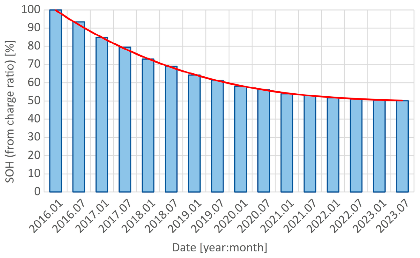
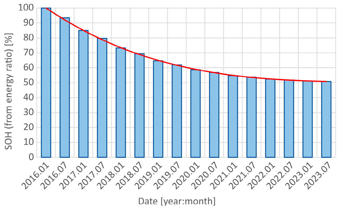
Results obtained from Equation (13) are shown in Figure 23, and results from Equation (14) are shown in Figure 24.

Data used for the SOH determination presented in Figure 23 and Figure 24 was obtained from the trend line shown in Figure 11 and Figure 12. Both figures show that the highest dynamics of the SOH degradation occurred in the first 2 years of vehicle operation. After the six and a half years of operation, the dynamics of SOH changes are practically negligible. The values of the SOH obtained from both Equations (13) and (14) converge at 51%. Both methods of determining the SOH based on the charge increase or on the energy increase during battery charging give similar results. Such information is of importance for the vehicle operator in the context of planning the timetable with consideration of Battery mode operation and energy efficiency improvement.

The third-degree polynomial approximates the SOH curve very well. The general form of this polynomial in the time domain is given by the equation

$$SOH\left(t\right)=a{t}^3+b{t}^2+ct+d$$

(15)

The t argument in Equation (15) starts with the value 0, which corresponds to the date 7 January 2016, i.e., the start date of data acquisition from the trolleybus. The subsequent values t = 1, 2, 3,…, represent the next days of trolleybus operation in relation to the date 7 January 2016. For the time argument defined in this way, the coefficients of this polynomial are given in

Table 4. Sets of coefficients for Equation (15).

Coefficient	SOC Criterion	Battery Voltage Criterion
a	−1.64384 × 10−9	−1.62959 × 10−9
b	1.5110371 × 10−5	1.49563635 × 10−5
c	−4.729856567 × 10−2	−4.677432272 × 10−2
d	100.531	99.832

. Two sets of coefficients are given: the first for the SOH determined from the SOC criterion (Figure 23) and the second for the SOH determined from the battery voltage criterion (Figure 24).

The values of these coefficients, especially those appearing before the time argument, must be quite precise. This is due to the fact that Equation (13) estimates the SOH for a relatively large time range (the number of days included in the 7-year battery life is counted in thousands). The number of days counted from 7 January 2016 to 1 June 2023 is over 2700.

7. Discussion of Selected Issues of the Presented Research Method

7.1. The Influence of the Specific SOC Intervals on the SOH Results of the Traction Battery

In order to analyse the influence of the SOC window on the SOH dynamics, studies were carried out for other SOC ranges. The following three SOC windows were analysed:

➢

Window 1 is SOC ∈ <SOC₁ = 60%; SOC₂ = 100%>,

➢

Window 2 is SOC ∈ <SOC₁ = 70%; SOC₂ = 100%>,

➢

Window 3 is SOC ∈ <SOC₁ = 80%; SOC₂ = 100%>

The results of the charge and energy delivered to the battery at Window 1 are shown in Figure 25 and Figure 26, respectively. At this SOC window, the sample set size is relatively small. The results for Window 2 are already presented in Figure 11 and Figure 12 in Chapter 4. The results of the charge and energy delivered to the battery at Window 3 are shown in Figure 27 and Figure 28, respectively. At this SOC window, the sample set size is relatively large, but the SOC window is narrow.

These figures also show the charge ratio $∆Q_1/∆Q_2$ and the energy ratio $∆E_1/∆E_2$, where index 1 refers to a new battery and index 2 to the battery condition after 6.5 years of operation. The percentage values of charge ratio and energy ratio for each SOC window are very similar (51–54%). This means that the SOH result is not sensitive to the SOC window size chosen for analysis, and the choice of the SOC range from 70% to 100% was a good compromise.

7.2. Practical Implementations of the Obtained Results

The practical implementation of the obtained results for the assessment of the SOH batteries in trolleybuses is closely related to the determined probability distributions f₁(x), f₂(x), f₃(x), f₄(x) and f₅(x) given by Equations (3), (4), (8), (9) and (11), respectively. The values of the parameters of these distributions determined in this work are of key importance for the implementation of the results on the SOH of NMC batteries of other trolleybuses. The conducted research has shown that if another trolleybus is to perform a public transport service and its histograms (minimum and maximum battery temperatures, discharge currents and new health indicator Q_OC/Q_1C) are well approximated by the corresponding distributions f₁(x), f₂(x), f₃(x), f₄(x) and f₅(x) with the parameters determined in this work, the dynamics of the SOH process will be practically the same.

In most electric vehicle applications, the battery life cycle (End-of-Life—EOL) is considered effective until it reaches 80% of its initial capacity. Taking this threshold into account, the operating time of the tested NMC battery to reach 80% of the initial capacity was approximately 18 months. This is a short battery life up to this EOL threshold. A number of factors influenced this condition:

➢

The number of charging cycles in Catenary mode in the first 18 months was about 270.

➢

The number of charging cycles in Catenary mode over 6.5 years was approximately 5800.

➢

Additionally, there were several thousand battery charges/discharges in Battery mode operation.

➢

The discharge current in Battery mode was relatively high—corresponding to 3C.

➢

The max battery temperature was relatively high—the aggregate number of maximum temperature intervals above 35 degrees was over 3000.

The battery, therefore, was operated in relatively difficult operating conditions.

On electrified lines, the trolleybus can be usually powered from the overhead lines. The battery is therefore necessary to operate on non-electrified lines to improve energy efficiency. Figure 2 shows that with a new battery (SOH close to 100%), the trolleybus could travel a distance of more than 80 km. With the SOH at approximately 50%, the trolleybus can travel a distance of approximately 40 km. This distance (40 km) is sufficient for public transport services operated by trolleybuses on partly non-electrified lines even in large urban agglomerations. Therefore, battery degradation to the SOH level of 50% in trolleybuses does not always have to mean the end of its service life.

Detailed SOH studies included several trolleybuses performing similar public transport tasks on partially the same and partially different routes. In each case, very similar SOH curve descent dynamics were observed. It is also significant that up to 6.5 years of battery operation, the rate of change ∆SOH per unit of time ∆t (few months), i.e., $\left|∆SOH/∆t\right|$, did not increase, but even decreased. No further tests were performed after 6.5 years of battery operation.

8. Conclusions

The trolleybus’s historical data constitute a very large database, whose base tables contain a daily collection of several dozen recorded values. The conclusions drawn from the analysis of the trolleybus’s historical data are as follows:

• In the battery operation mode, most cases (over 200 cases) of the distance covered were found in the 45–50 km class range. Distribution of distance covered (around 100 runs) occurred in a relatively wide class range of 10–35 km.
• The empirical distribution of the relative value of energy regenerated into the grid by trolleybuses indicates that most often (250 to 300 cases), the RVE/IVE parameter ranged from 5% to 17.5%.
• The empirical distribution of the relative value of regenerative braking energy indicates that most often (in over 550 cases), it concerned the RDE/IDE parameter in the range of 35% to 37%.
• For the analysis of the battery SOH, two criteria were specified: the SOC criterion—SOC ∈ <SOC₁ = 70%, SOC₂ = 100%>, and the voltage criterion—U_batt ∈ <U_batt1 = 650 V, U_batt2 = 680 V>.
• The algorithm found from a few to over a dozen cases fulfilling the stated criteria for each daily dataset.
• Under the specified criteria, the charge and energy supplied to the battery decreases as a function of operation time. The dynamics of those changes are the greatest in the first 2 years of operation. In the first half of the 7th year of operation, the changes are less prominent.
• The trend line defined using the 3rd degree polynomial approximates relatively well the results of the charge and energy supplied to the battery in Catenary mode.
• For determining the SOH of the battery, equations using increments of the charge and energy supplied to the battery under the same criteria as the daily acquisition dataset were utilised.
• The dynamics of the SOH decrease was the highest in the first 2 years of the trolleybus operation. After six and a half; years, the dynamics of the SOH change are practically negligible. Value of the SOH obtained from equations converges at 51%.
• The empirical distribution of minimum and maximum battery temperatures is well approximated by the normal distribution.
• The empirical charge distribution of Q_1C (charge to 1C) and Q_OC (charge over 1C) in driving mode is well approximated by the Gamma distribution.
• The obtained approximations f₁(x), f₂(x), f₃(x), f₄(x) and f₅(x) of the empirical distributions may be helpful in assessing the SOH of Li-ion NMC batteries installed in other trolleybuses.
• Statistical analysis of significant empirical distributions (temperature, current, etc.) of a trolleybus operating under actual operating conditions is crucial for assessing the SOH of a battery. Determining distributions that approximate the empirical distributions relatively well allows for determining the relationship between the distribution parameters (mean value, variance, kurtosis, skewness, etc.) and the SOH curve.