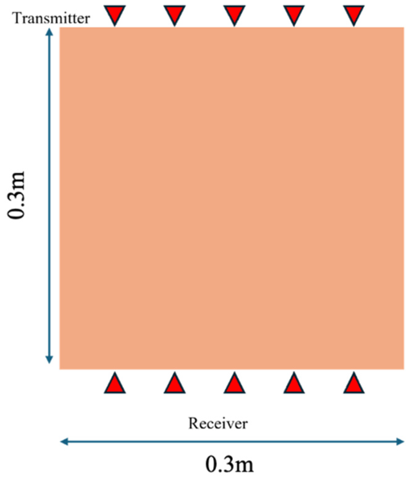
Figure 1.
Measurement setup. The orange region represents sandstone indicated. The red triangles denote the receiver and transmitter antennas.
Figure 1.
Measurement setup. The orange region represents sandstone indicated. The red triangles denote the receiver and transmitter antennas.
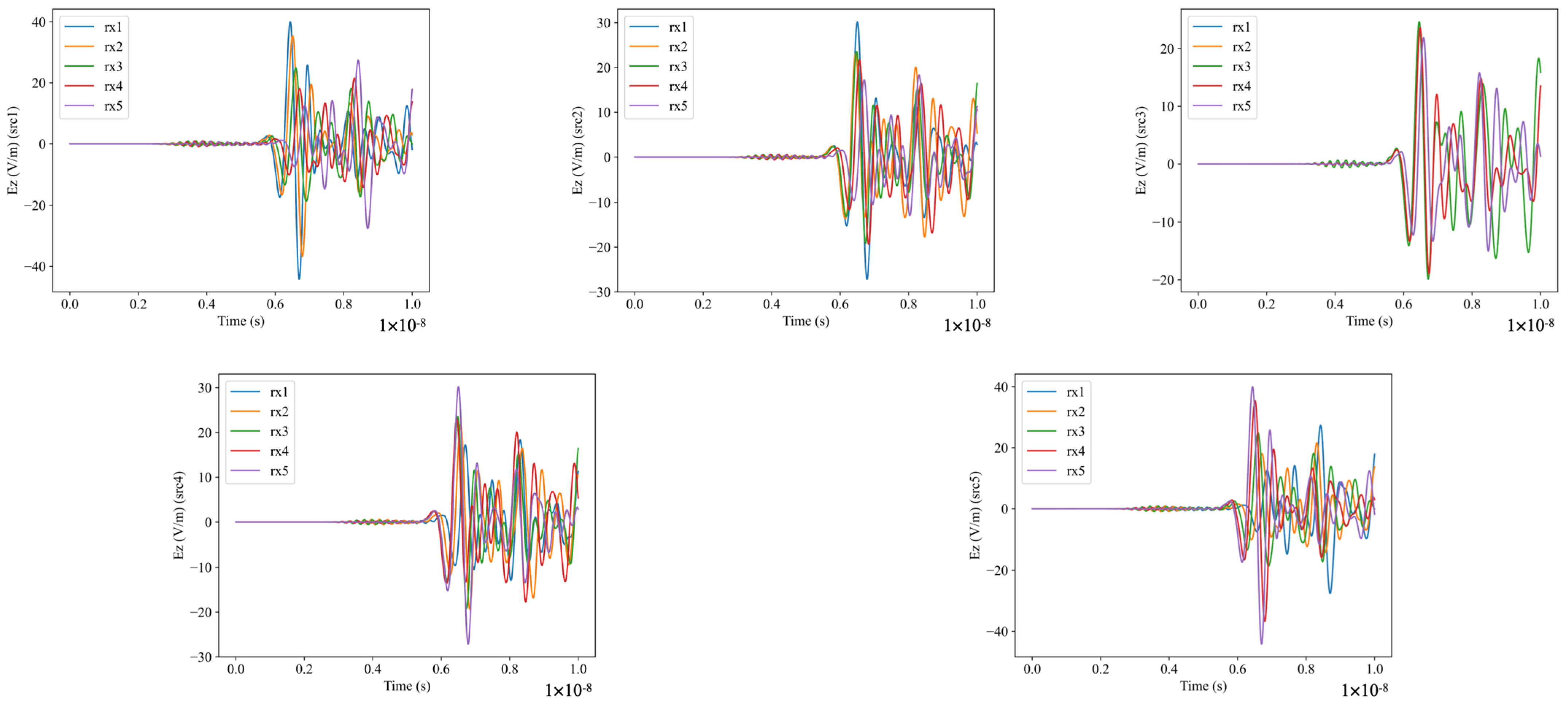
Figure 2.
Forward simulation results from the gprMax software, where src1, src2, src3, src4, and src5 represent the first to the fifth transmitter antennas, and rx1, rx2, rx3, rx4, and rx5 represent the first to the fifth receiver antennas.
Figure 2.
Forward simulation results from the gprMax software, where src1, src2, src3, src4, and src5 represent the first to the fifth transmitter antennas, and rx1, rx2, rx3, rx4, and rx5 represent the first to the fifth receiver antennas.
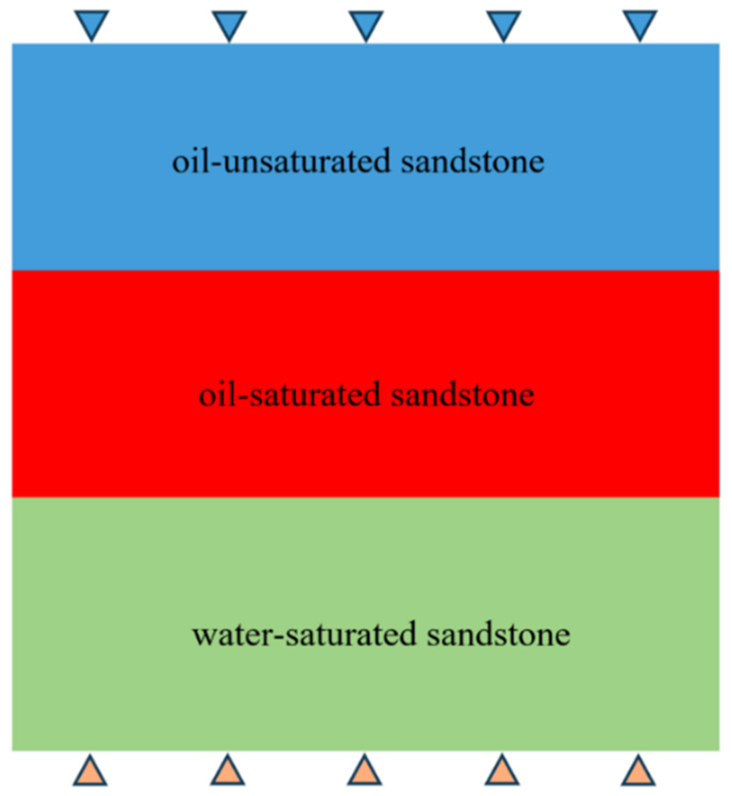
Figure 3.
Distribution of different media states at different stages of flooding. The blue triangle represents the transmitter and the orange triangle indicates the receivers.
Figure 3.
Distribution of different media states at different stages of flooding. The blue triangle represents the transmitter and the orange triangle indicates the receivers.
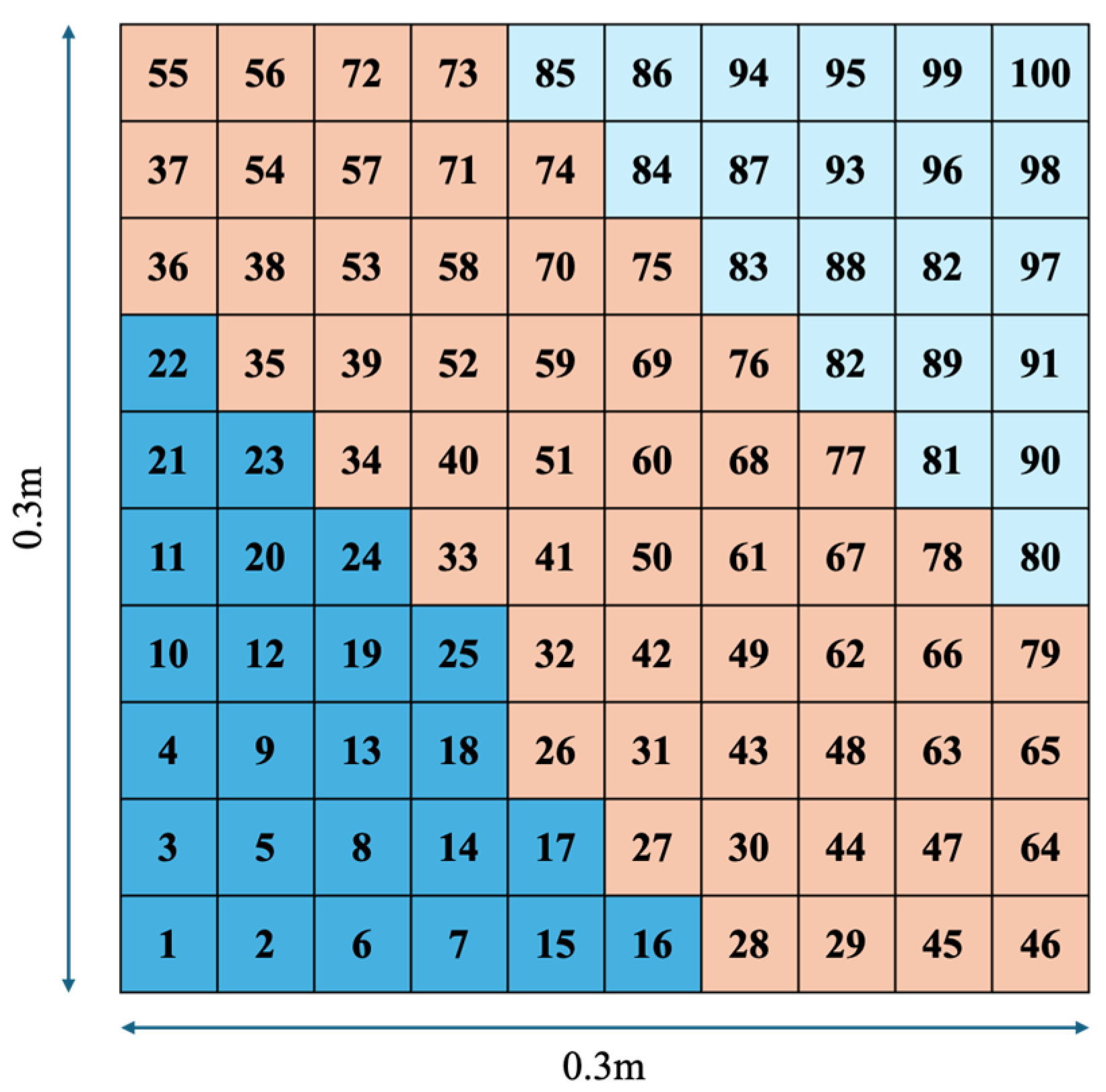
Figure 4.
Simulation of different stages of oil–water flooding. Dark blue represents the water-rich zone, yellow represents the oil-rich zone, and sky blue represents the original rock.
Figure 4.
Simulation of different stages of oil–water flooding. Dark blue represents the water-rich zone, yellow represents the oil-rich zone, and sky blue represents the original rock.
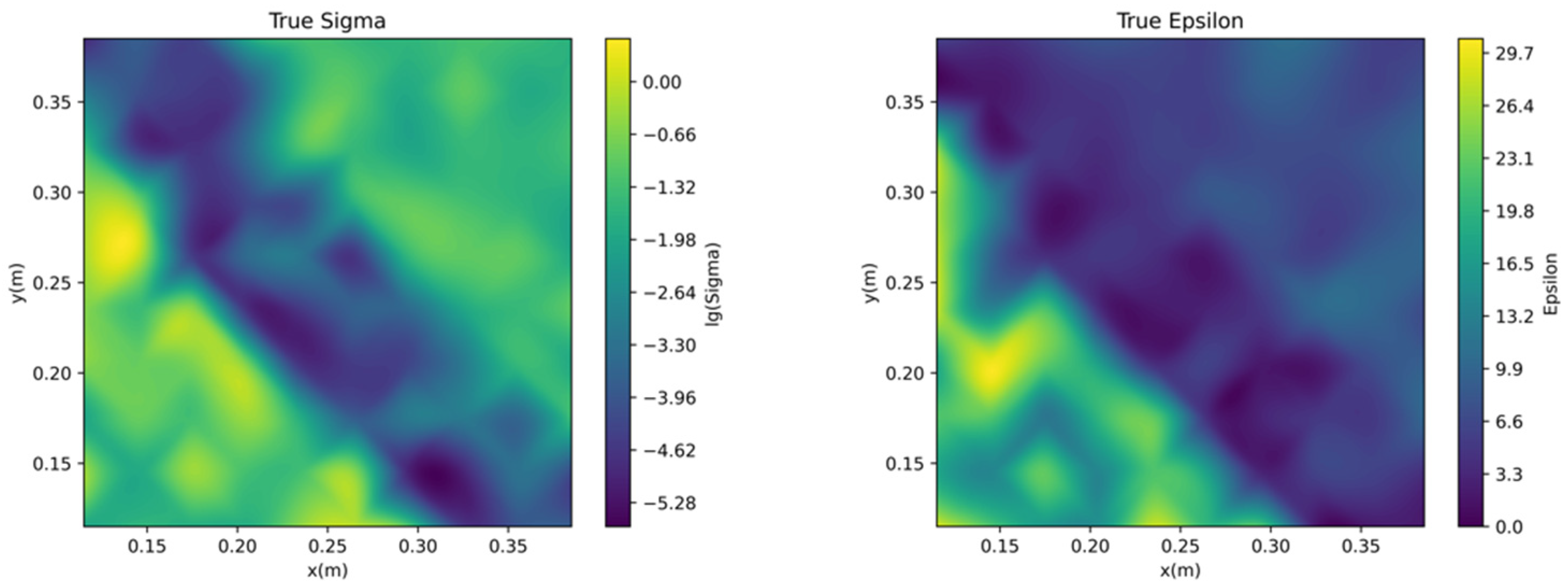
Figure 5.
The conductivity and dielectric constant distribution map, where the (left panel) is about the logarithmic conductivity distribution and the (right panel) shows the dielectric constant distribution.
Figure 5.
The conductivity and dielectric constant distribution map, where the (left panel) is about the logarithmic conductivity distribution and the (right panel) shows the dielectric constant distribution.
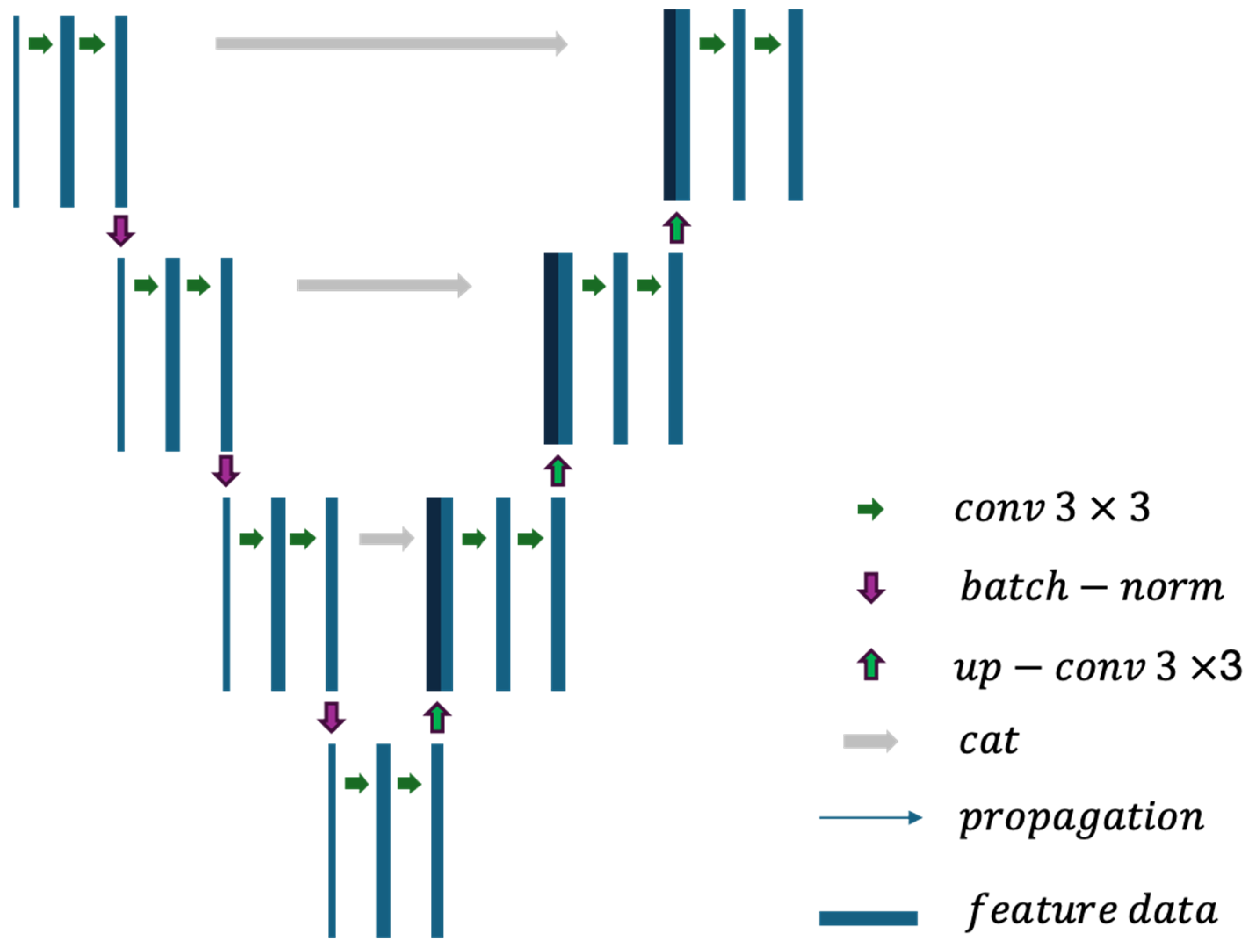
Figure 6.
Schematic diagram of the U-Net neural network structure.
Figure 6.
Schematic diagram of the U-Net neural network structure.
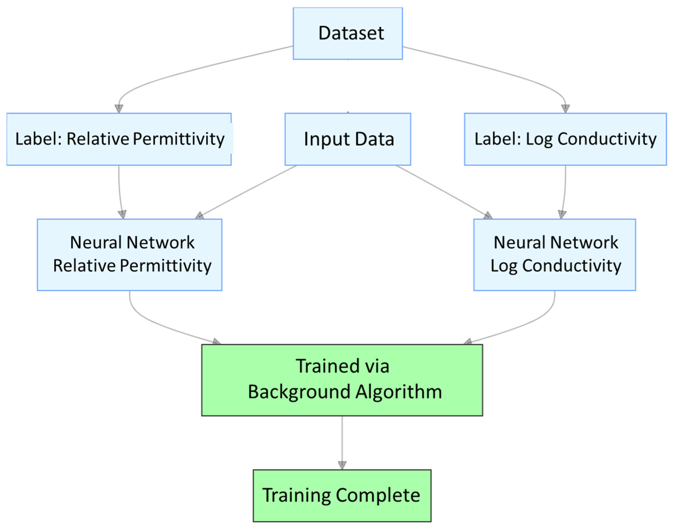
Figure 7.
Inversion neural network training flowchart.
Figure 7.
Inversion neural network training flowchart.
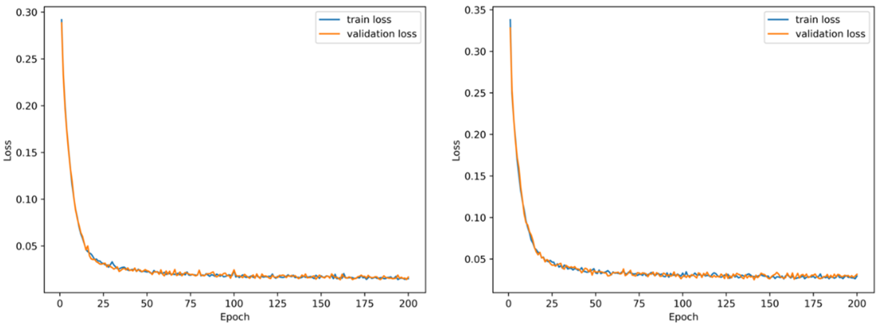
Figure 8.
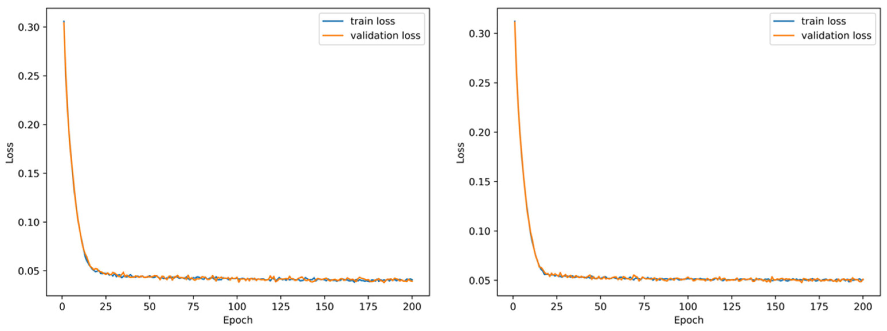
Loss function decay curves for Dataset 1. The (left graph) shows the decay curve for the dielectric constant inversion network, and the (right graph) shows the decay curve for the resistivity inversion network.
Figure 8.
Loss function decay curves for Dataset 1. The (left graph) shows the decay curve for the dielectric constant inversion network, and the (right graph) shows the decay curve for the resistivity inversion network.
Figure 9.
Loss function decay curves for Dataset 2. The (left graph) shows the decay curve for the dielectric constant inversion network, and the (right graph) shows the decay curve for the resistivity inversion network.
Figure 9.
Loss function decay curves for Dataset 2. The (left graph) shows the decay curve for the dielectric constant inversion network, and the (right graph) shows the decay curve for the resistivity inversion network.
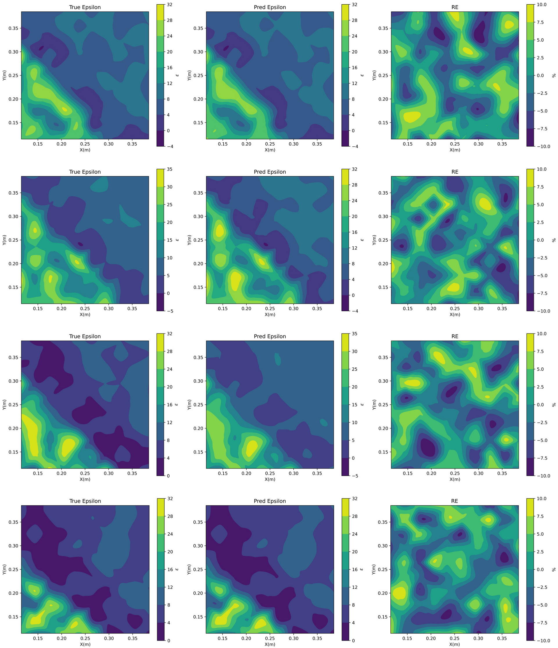
Figure 10.
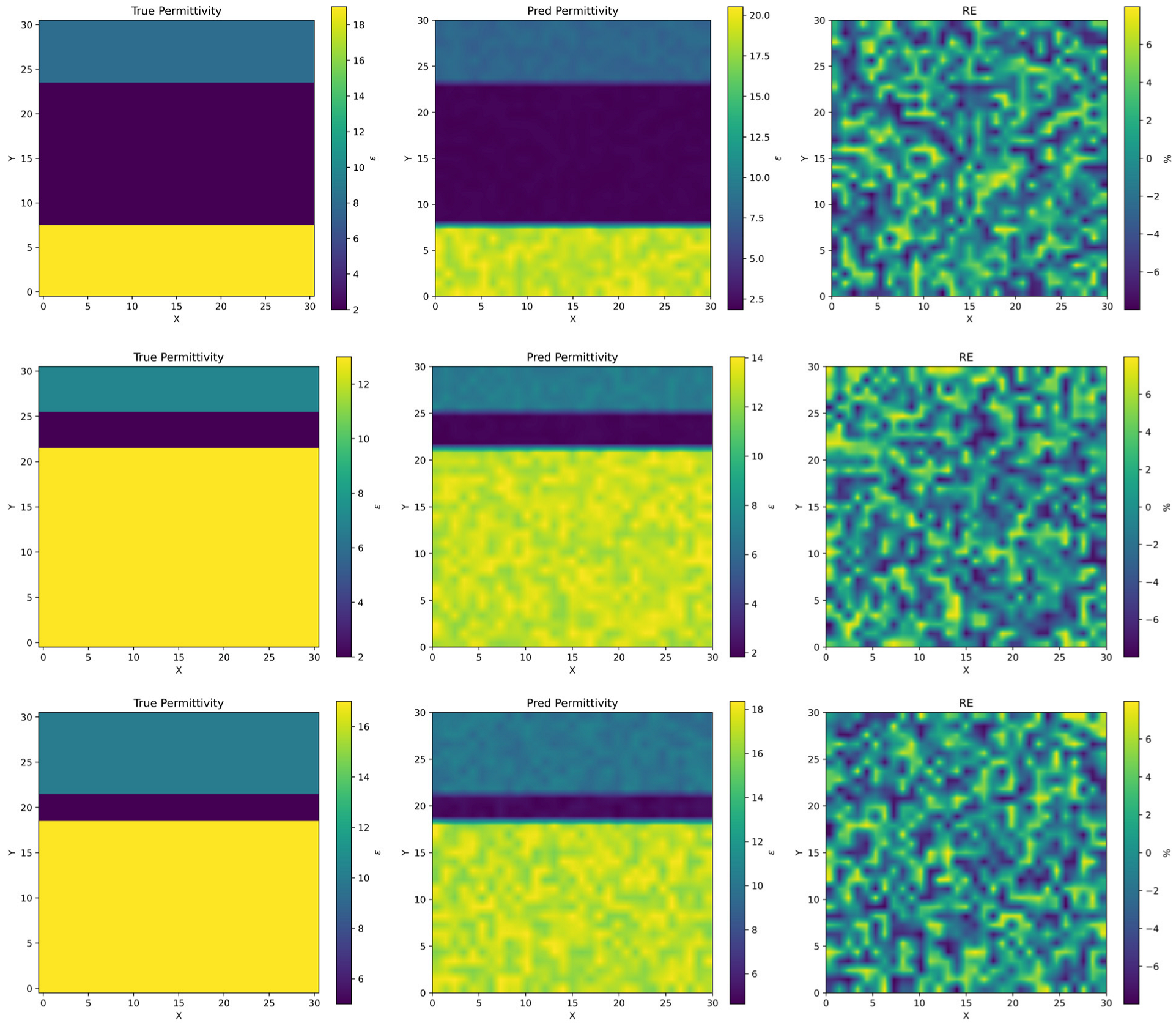
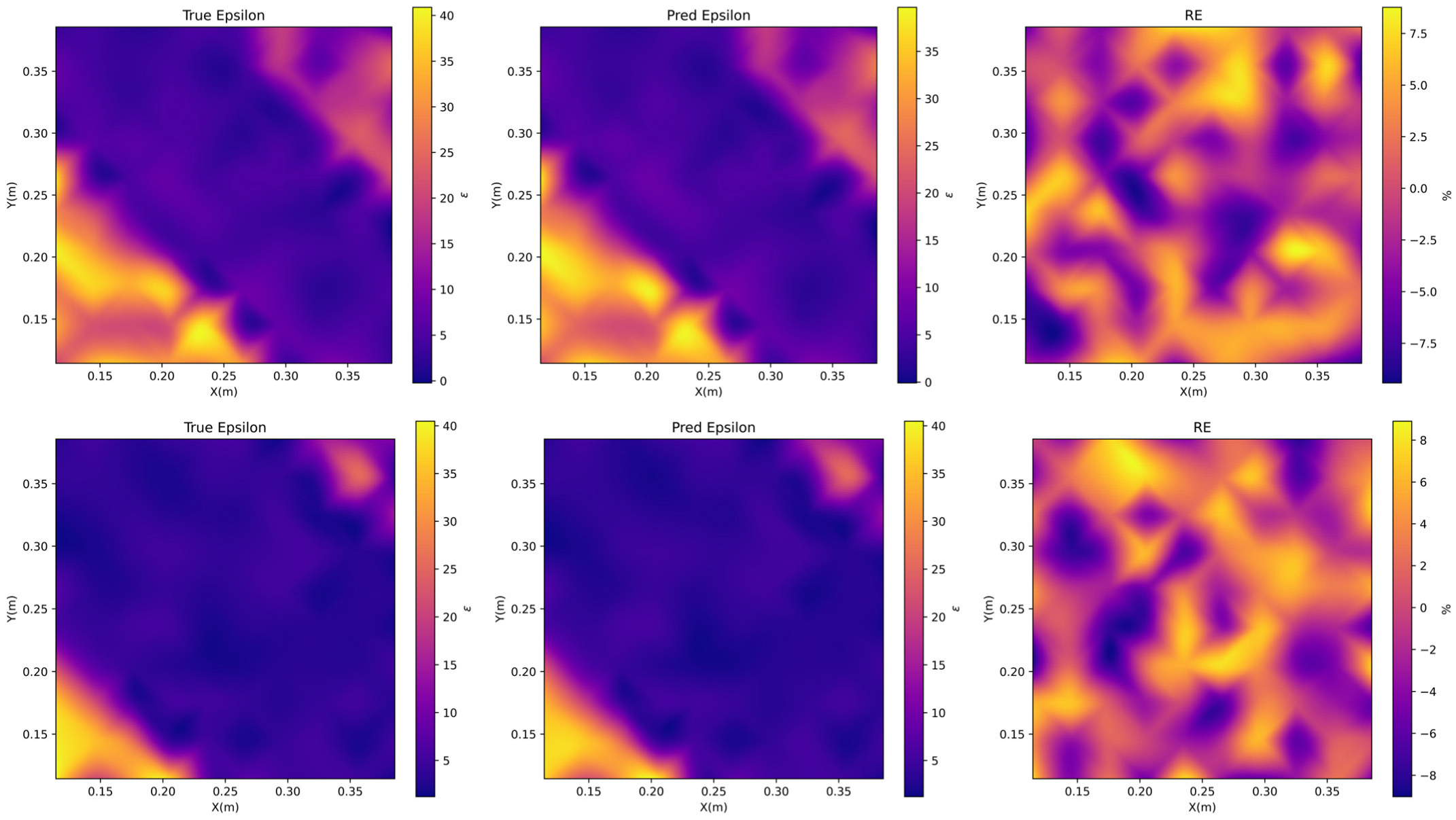
2D dielectric constant inversion results of three randomly selected synthetic models, where the first, second, and third layer is from three models, and the first, second, and third column is the true dielectric constant, inversion results, and the relative errors, respectively.
Figure 10.
2D dielectric constant inversion results of three randomly selected synthetic models, where the first, second, and third layer is from three models, and the first, second, and third column is the true dielectric constant, inversion results, and the relative errors, respectively.
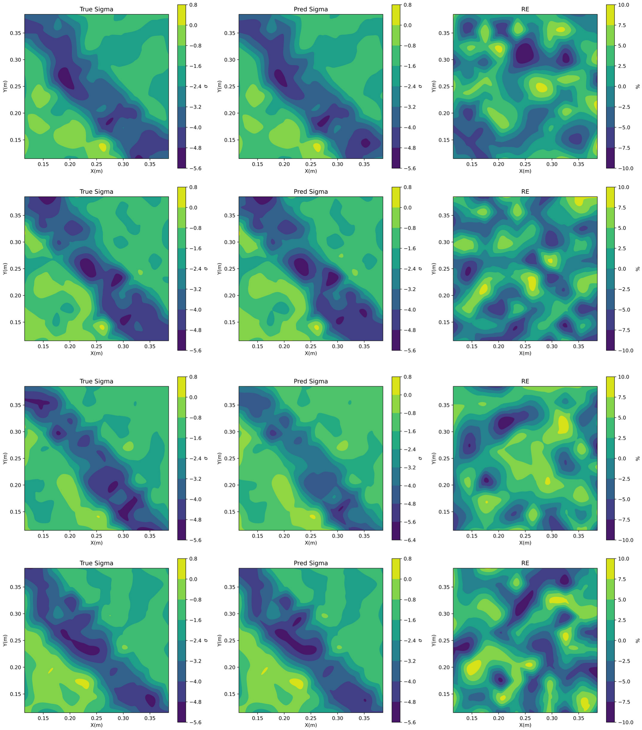
Figure 11.
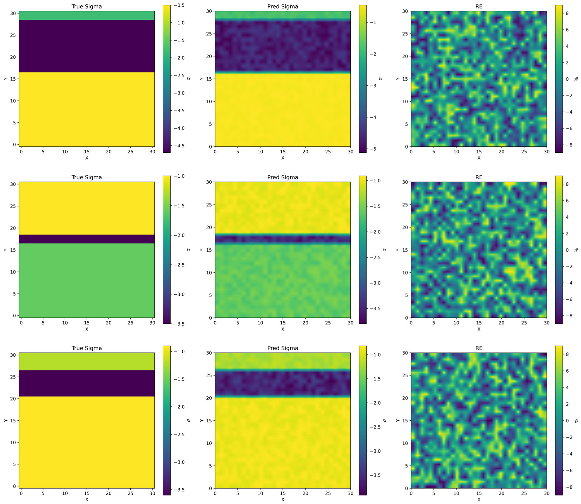
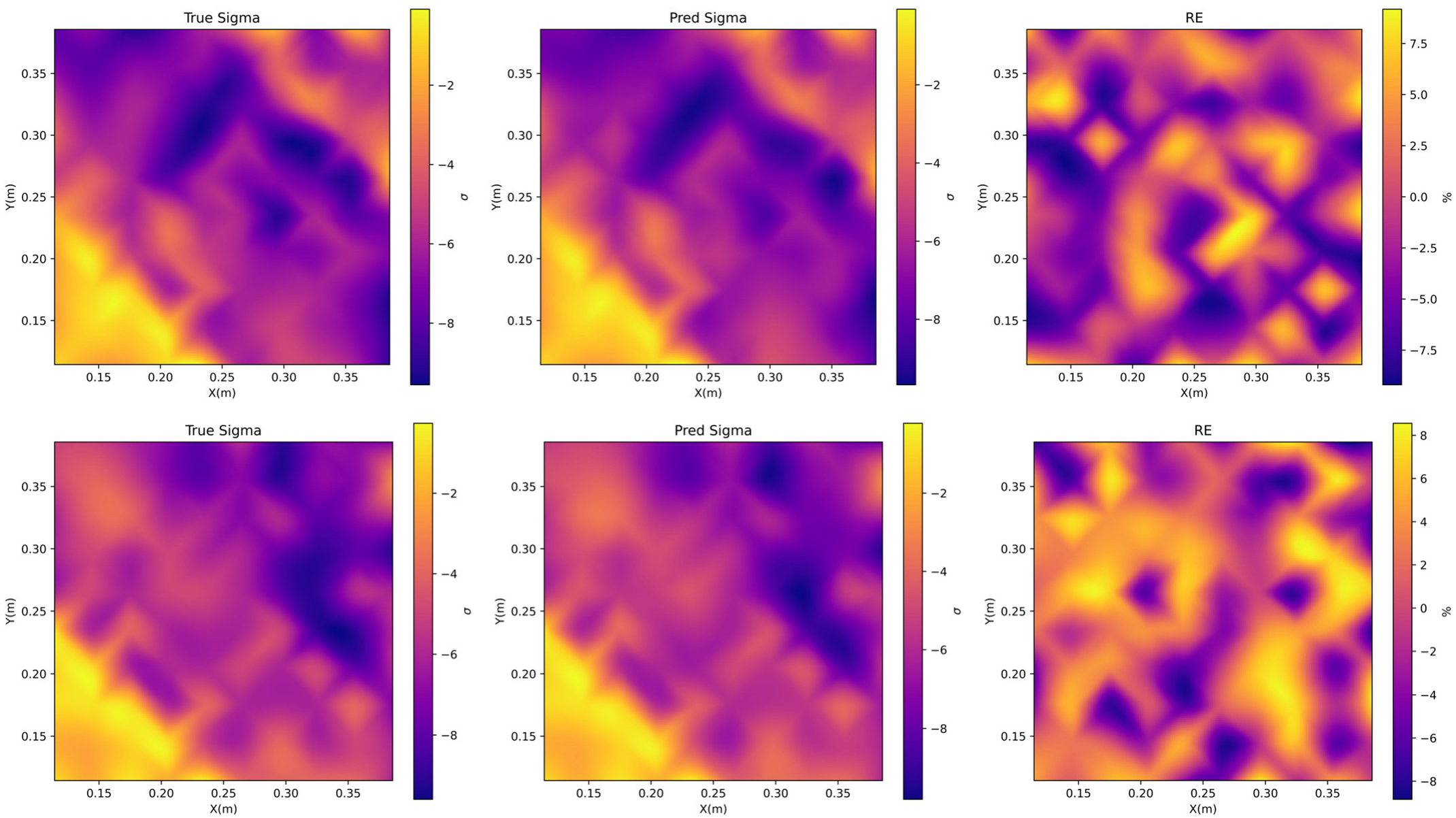
2D conductivity inversion results for the model of three randomly selected synthetic models, where the first, second, and third layer are from three models, and the first, second, and third column is the true conductivity, inversion results, and the relative errors, respectively.
Figure 11.
2D conductivity inversion results for the model of three randomly selected synthetic models, where the first, second, and third layer are from three models, and the first, second, and third column is the true conductivity, inversion results, and the relative errors, respectively.
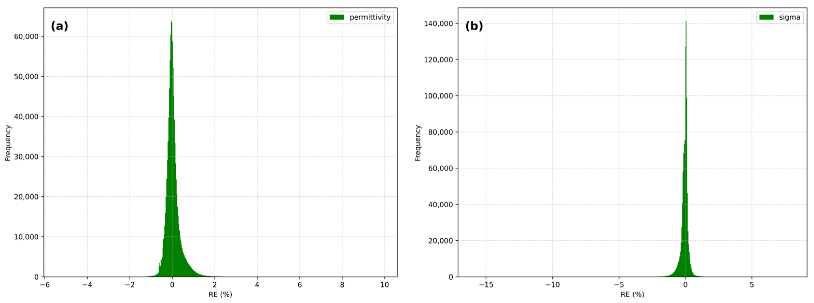
Figure 12.
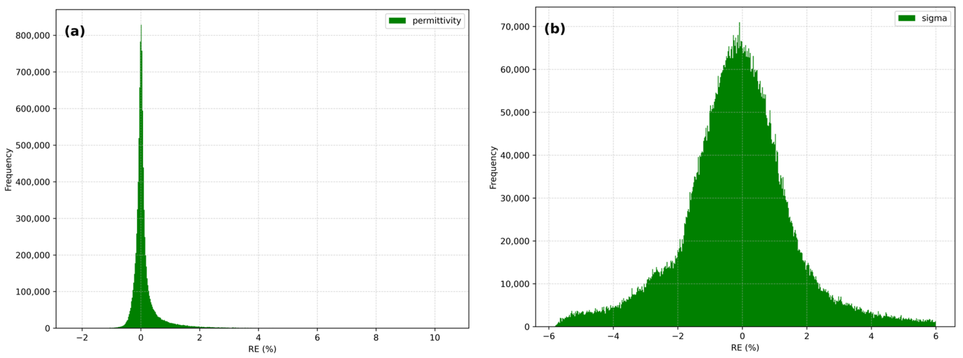
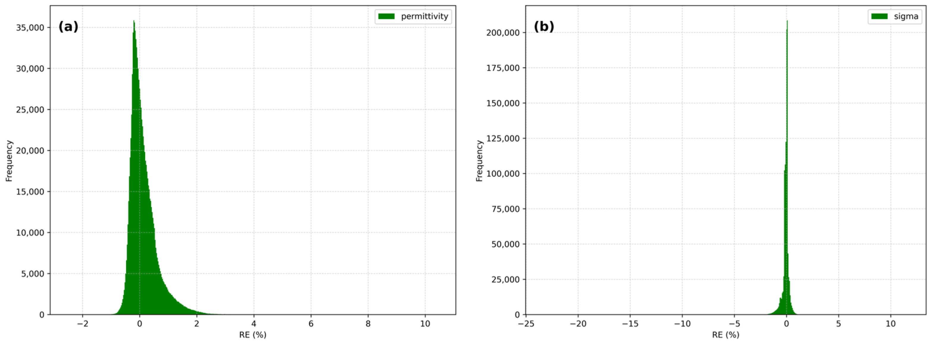
Relative error distribution of the test set: (a) permittivity; (b) conductivity.
Figure 12.
Relative error distribution of the test set: (a) permittivity; (b) conductivity.
Figure 13.
2D dielectric constant inversion results for the model. Each row of three images represents the inversion results for different models. The left column image shows the true dielectric constant distribution, the middle column image shows the inverted dielectric constant distribution, and the right column image shows the relative error distribution of the inversion results.
Figure 13.
2D dielectric constant inversion results for the model. Each row of three images represents the inversion results for different models. The left column image shows the true dielectric constant distribution, the middle column image shows the inverted dielectric constant distribution, and the right column image shows the relative error distribution of the inversion results.
Figure 14.
2D conductivity inversion results for the model. Each row of three images represents the inversion results for different models. The left column image shows the true conductivity distribution, the middle column image shows the inverted conductivity distribution, and the right column image shows the relative error distribution of the inversion results.
Figure 14.
2D conductivity inversion results for the model. Each row of three images represents the inversion results for different models. The left column image shows the true conductivity distribution, the middle column image shows the inverted conductivity distribution, and the right column image shows the relative error distribution of the inversion results.
Figure 15.
Average relative error distribution for the inversion results of the testing set. The left graph shows the relative dielectric constant, and the right graph shows the relative conductivity.
Figure 15.
Average relative error distribution for the inversion results of the testing set. The left graph shows the relative dielectric constant, and the right graph shows the relative conductivity.
Figure 16.
Relative error distribution of the test set: (a) permittivity; (b) conductivity.
Figure 16.
Relative error distribution of the test set: (a) permittivity; (b) conductivity.
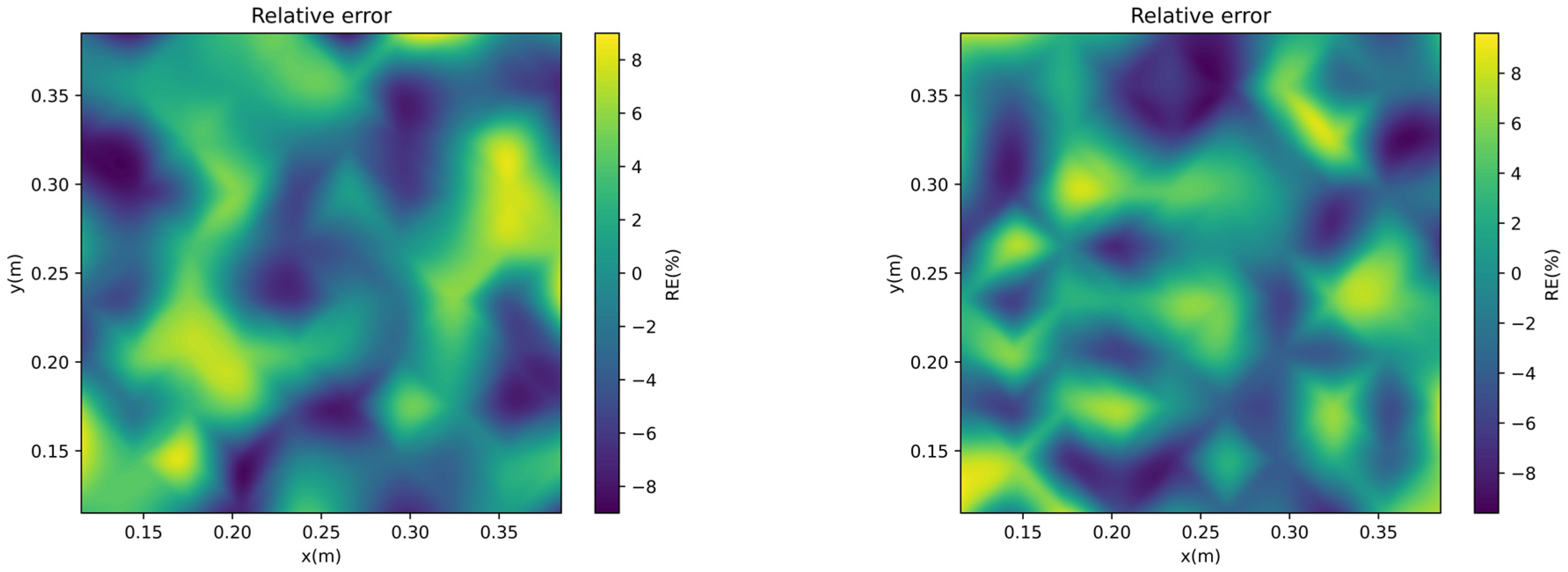
Figure 17.
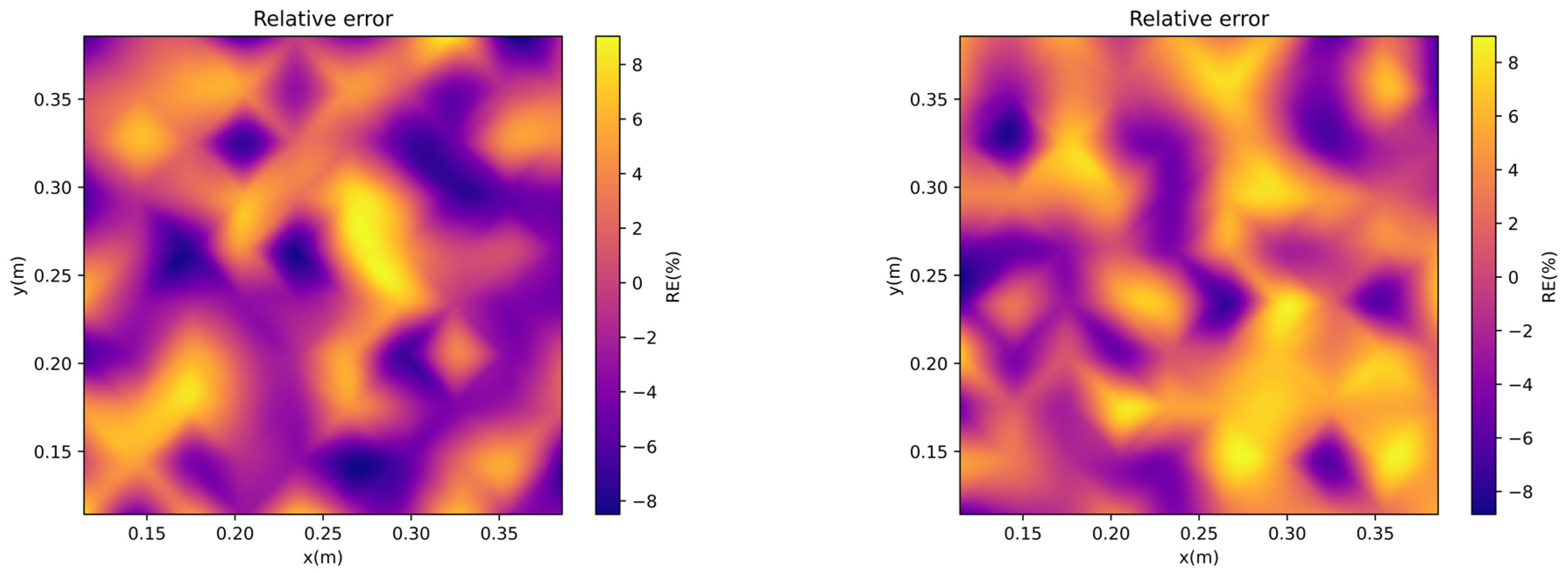
Spatial distribution maps of average relative error for the test set. The left panel corresponds to the relative errors of the permittivity, and the right panel is about that of the electrical conductivity in the logarithm scale.
Figure 17.
Spatial distribution maps of average relative error for the test set. The left panel corresponds to the relative errors of the permittivity, and the right panel is about that of the electrical conductivity in the logarithm scale.
Figure 18.
2D inversion results for a random model. Each row of three images represents the inversion results for different models. The left image shows the true distribution, the middle image shows the inverted distribution, and the right image shows the relative error distribution of the inversion results. The first row is about the distributions of permittivity, and the second row is about the conductivity distributions.
Figure 18.
2D inversion results for a random model. Each row of three images represents the inversion results for different models. The left image shows the true distribution, the middle image shows the inverted distribution, and the right image shows the relative error distribution of the inversion results. The first row is about the distributions of permittivity, and the second row is about the conductivity distributions.
Figure 19.
2D inversion results for another random model. Each row of three images represents the inversion results for different models. The left image shows the true distribution, the middle image shows the inverted distribution, and the right image shows the relative error distribution of the inversion results. The first row is about the distributions of permittivity, and the second row is about the conductivity distributions.
Figure 19.
2D inversion results for another random model. Each row of three images represents the inversion results for different models. The left image shows the true distribution, the middle image shows the inverted distribution, and the right image shows the relative error distribution of the inversion results. The first row is about the distributions of permittivity, and the second row is about the conductivity distributions.
Figure 20.
Relative error distribution of the test set: (a) permittivity; (b) conductivity.
Figure 20.
Relative error distribution of the test set: (a) permittivity; (b) conductivity.
Figure 21.
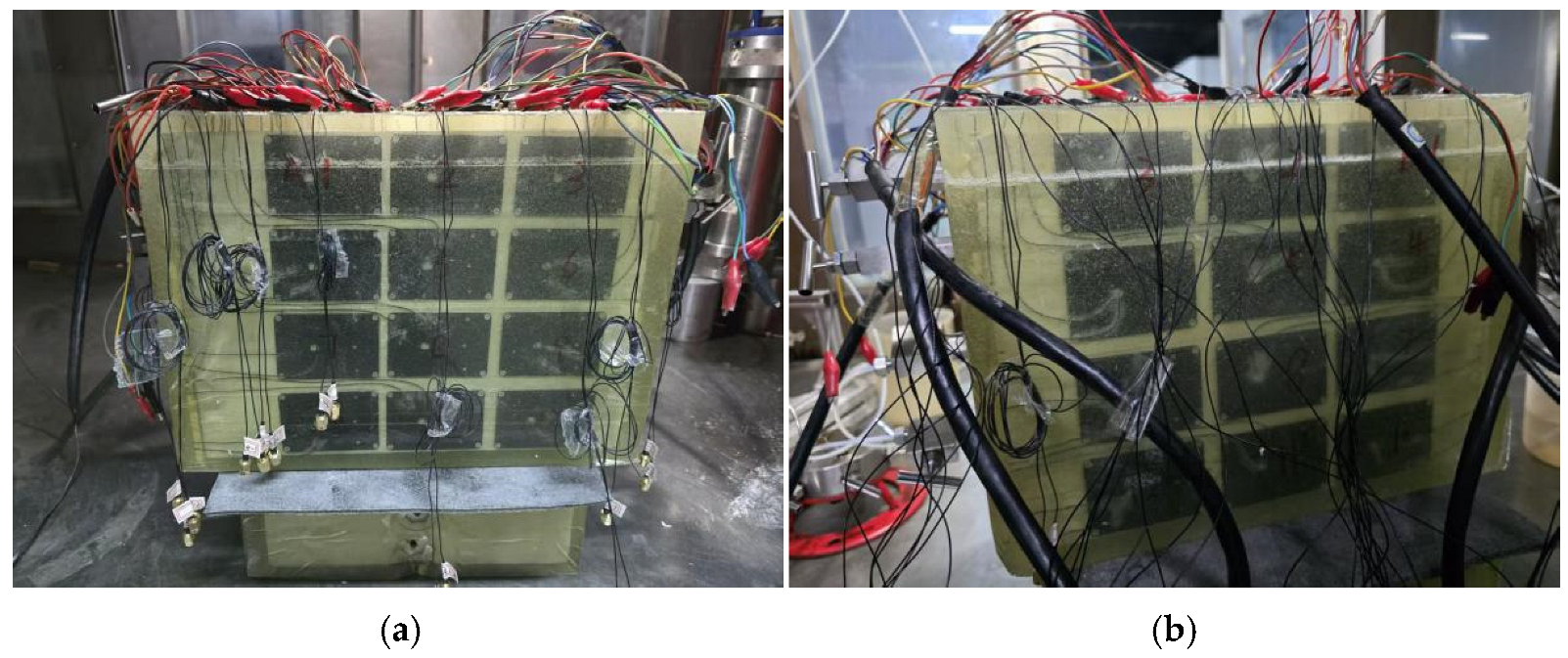
The observation system of the physical core flooding experiment. (a) 12 transmitters distributed on one side of the core, (b) 12 receivers distributed on another side of the core.
Figure 21.
The observation system of the physical core flooding experiment. (a) 12 transmitters distributed on one side of the core, (b) 12 receivers distributed on another side of the core.
Figure 22.
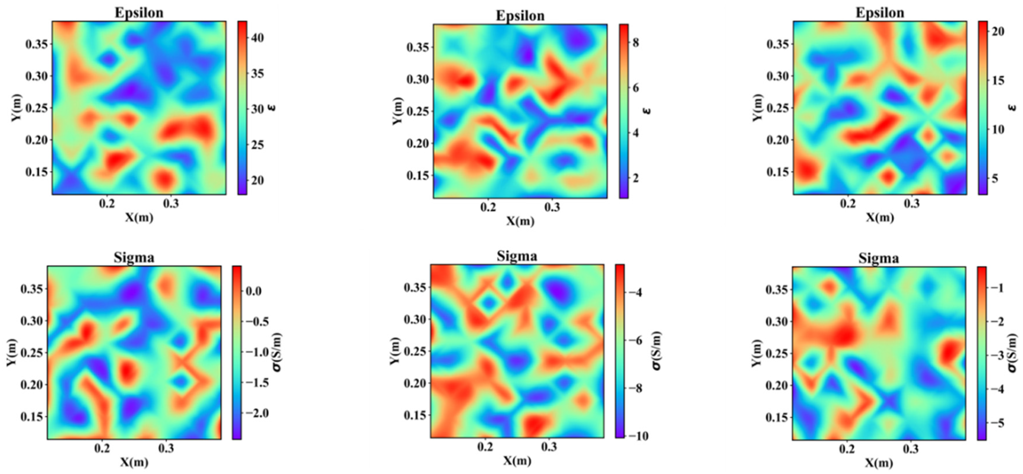
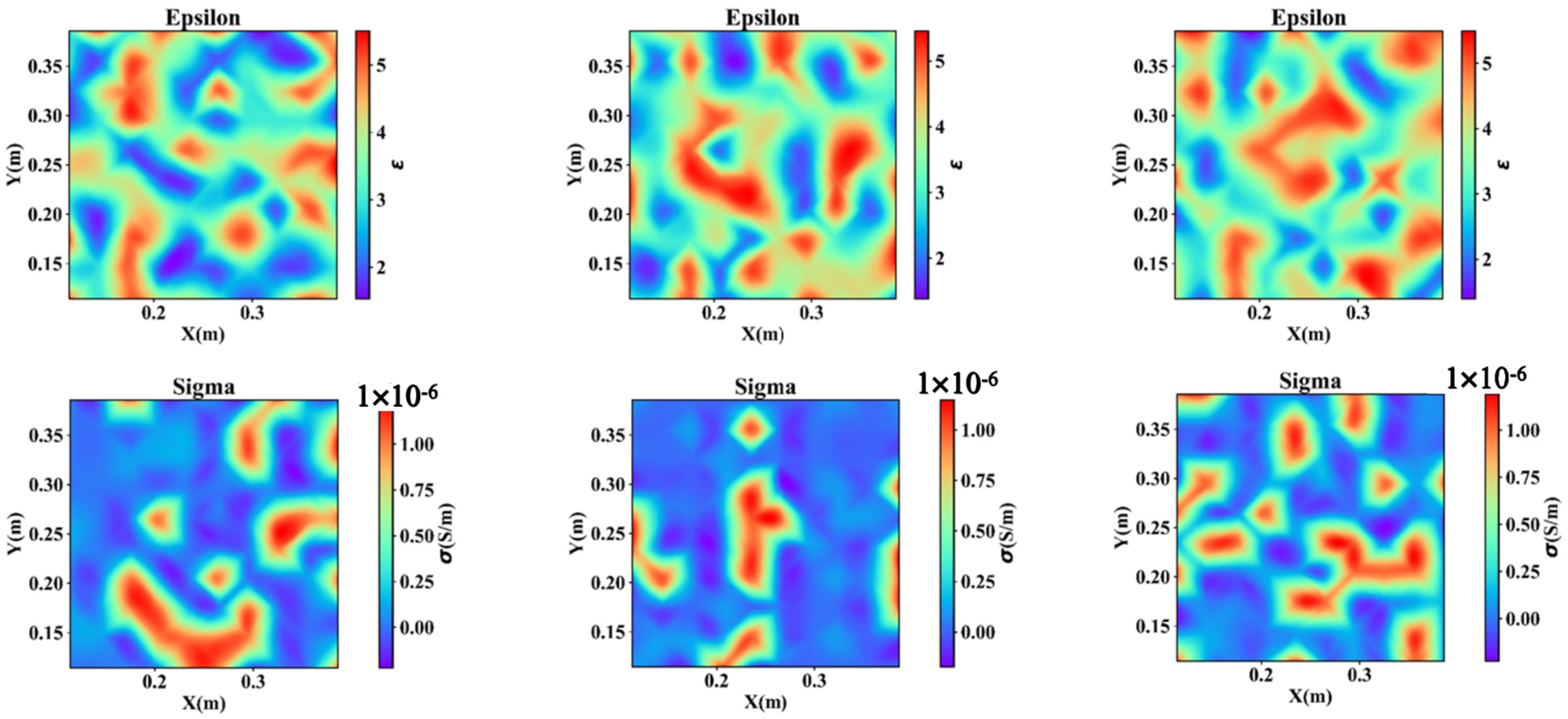
2D inversion results in the starting stage of the water flooding oil experiment done in a laboratory rock core. The first row shows the variations in the electric permittivity distribution in different slices of the core, and the second row shows the variations in the conductivity distribution in different slices of the core.
Figure 22.
2D inversion results in the starting stage of the water flooding oil experiment done in a laboratory rock core. The first row shows the variations in the electric permittivity distribution in different slices of the core, and the second row shows the variations in the conductivity distribution in different slices of the core.
Figure 23.
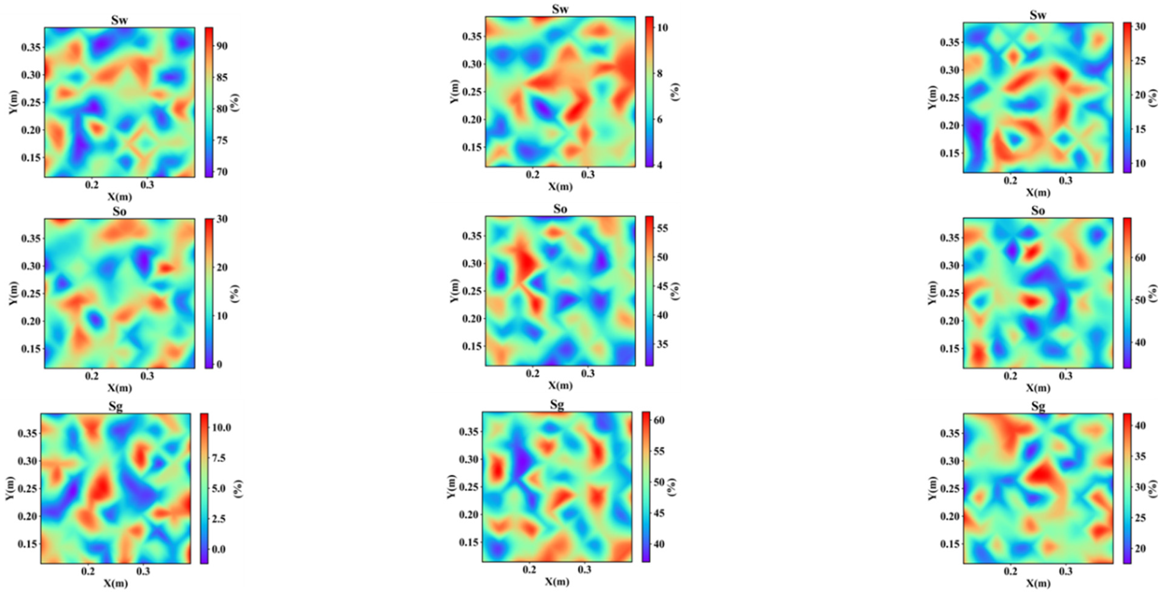
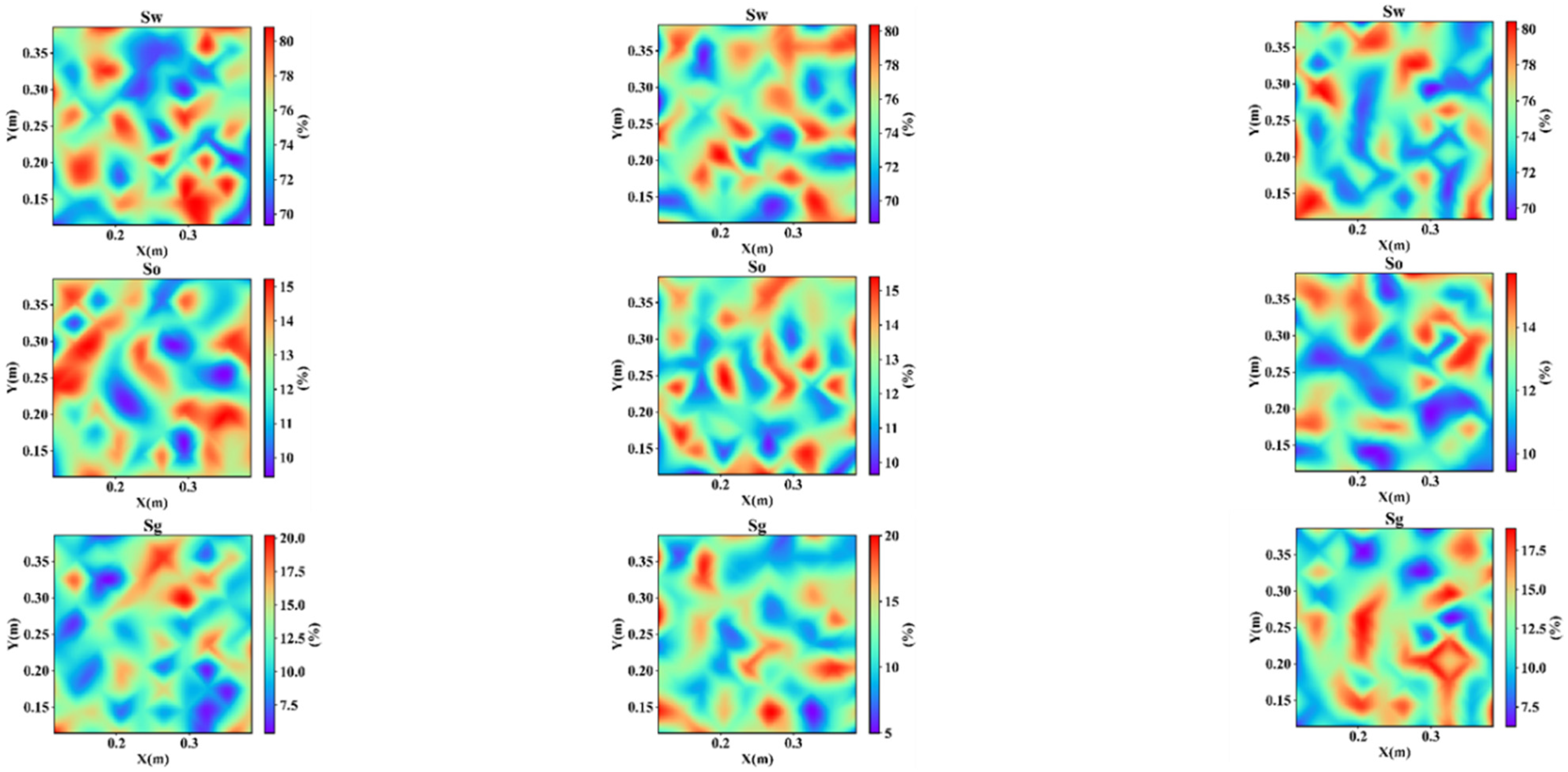
2D saturation results in the starting stage of the water flooding oil experiment done in a laboratory rock core. The first row shows the water saturation distribution in different slices of the core, the second row shows the oil saturation distribution in different slices of the core, and the third row shows the gas saturation distribution in different slices of the core.
Figure 23.
2D saturation results in the starting stage of the water flooding oil experiment done in a laboratory rock core. The first row shows the water saturation distribution in different slices of the core, the second row shows the oil saturation distribution in different slices of the core, and the third row shows the gas saturation distribution in different slices of the core.
Figure 24.
2D inversion results at the beginning of the air flooding water experiment done in a laboratory rock core. The first row shows the variations in the electric permittivity distribution in different slices of the core, and the second row shows the variations in the conductivity distribution in different slices of the core.
Figure 24.
2D inversion results at the beginning of the air flooding water experiment done in a laboratory rock core. The first row shows the variations in the electric permittivity distribution in different slices of the core, and the second row shows the variations in the conductivity distribution in different slices of the core.
Figure 25.
2D saturation results in the starting stage of the air flooding water experiment done in a laboratory rock core. The first row shows the water saturation distribution in different slices of the core, the second row shows the oil saturation distribution in different slices of the core, and the third row shows the gas saturation distribution in different slices of the core.
Figure 25.
2D saturation results in the starting stage of the air flooding water experiment done in a laboratory rock core. The first row shows the water saturation distribution in different slices of the core, the second row shows the oil saturation distribution in different slices of the core, and the third row shows the gas saturation distribution in different slices of the core.
Figure 26.
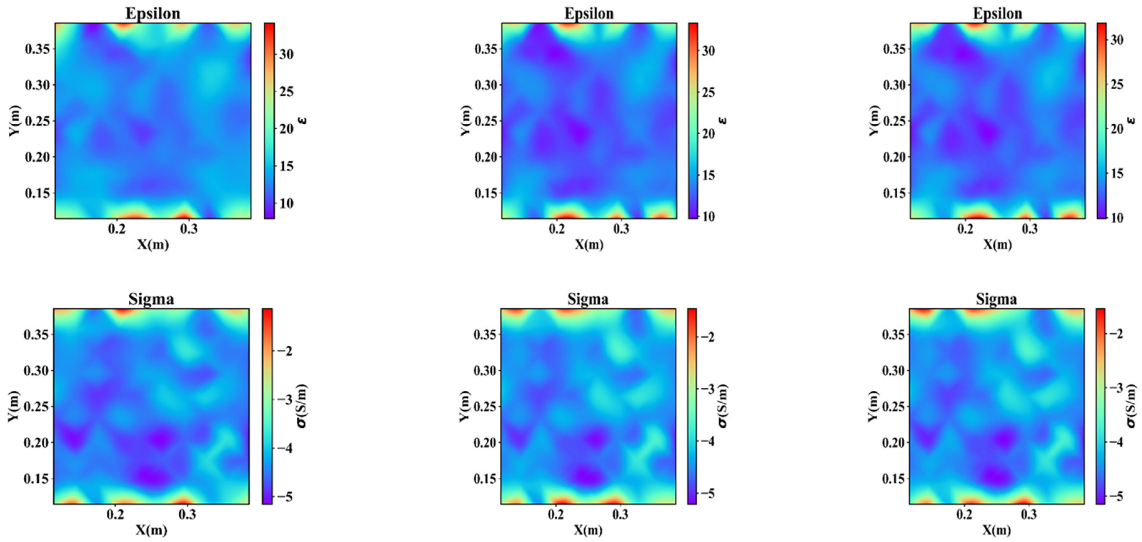
2D inversion results at the end of the air flooding water experiment done in a laboratory rock core. The first row shows the variations in the electric permittivity distribution in different slices of the core, and the second row shows the variations in the conductivity distribution in different slices of the core.
Figure 26.
2D inversion results at the end of the air flooding water experiment done in a laboratory rock core. The first row shows the variations in the electric permittivity distribution in different slices of the core, and the second row shows the variations in the conductivity distribution in different slices of the core.
Figure 27.
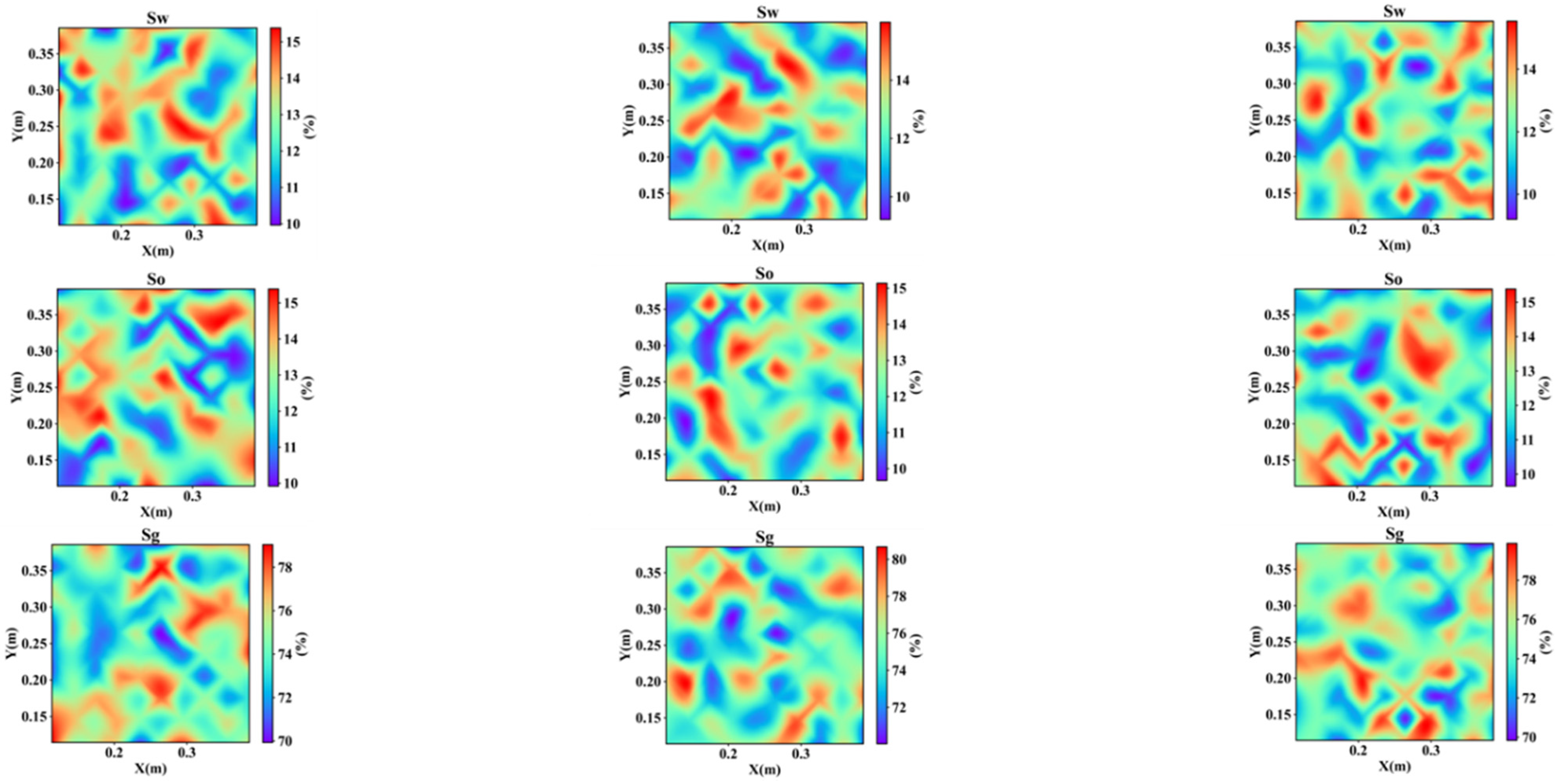
2D saturation results in the end stage of the gas flooding water experiment done in a laboratory rock core. The first row shows the water saturation distribution in different slices of the core, the second row shows the oil saturation distribution in different slices of the core, and the third row shows the gas saturation distribution in different slices of the core.
Figure 27.
2D saturation results in the end stage of the gas flooding water experiment done in a laboratory rock core. The first row shows the water saturation distribution in different slices of the core, the second row shows the oil saturation distribution in different slices of the core, and the third row shows the gas saturation distribution in different slices of the core.
Table 1.
Value ranges and step sizes of different parameters.
Table 1.
Value ranges and step sizes of different parameters.
| Water | Oil | Sandstone | Water–Oil Interface | Oil–Sandstone Interface |
|---|
| Dielectric Constant | Conductivity | Dielectric Constant | Conductivity | Dielectric Constant | Conductivity | cm | cm |
|---|
| 10~30 | −2~0 | 2~6 | −5~−3 | 6–10 | −2~−1 | 10~40 | 10~40 |
| 1 | 0.1 | 1 | 0.1 | 1 | 0.1 | 1 | 1 |
Table 2.
Range of dielectric constants and conductivities for different substances (conductivity in logarithmic values).
Table 2.
Range of dielectric constants and conductivities for different substances (conductivity in logarithmic values).
| Water | Oil | Sandstone |
|---|
| Dielectric Constant | Conductivity | Dielectric Constant | Conductivity | Dielectric Constant | Conductivity |
|---|
| 10~30 | −2~0 | 2~6 | −5~−3 | 6–10 | −2~−1 |
| 1 | 0.1 | 1 | 0.1 | 1 | 0.1 |
Table 3.
Neural network hyperparameters.
Table 3.
Neural network hyperparameters.
| Learning Rate | Batch Size | Epochs | Activation Function | Optimization Algorithm | Regularization |
|---|
| 1 × 10⁻⁴ | 128 | 200 | Tanh | Adam | L2 |