Article

On the Use of Clarke Transformation for the Transient Analysis of Asymmetrical Faults in Three-Phase Power Systems


Department of Electronics, Information and Bioengineering, Politecnico di Milano, 20133 Milan, Italy
Energies 2026, 19(11), 2580; https://doi.org/10.3390/en19112580
Submission received: 29 April 2026 / Revised: 17 May 2026 / Accepted: 25 May 2026 / Published: 27 May 2026
(This article belongs to the Special Issue Modeling and Analysis of Power Systems)

Abstract

This work provides a theoretical/methodological contribution to the transient analysis of asymmetrical faults in three-phase systems. Transient analysis of three-phase systems is usually performed by resorting either to the instantaneous Symmetrical Component Transformation (SCT) or to numerical methods. In this paper, an analytical methodology based on the time-domain Clarke transformation is presented for the transient analysis of the most common asymmetrical faults. For each kind of asymmetrical fault, a specific circuit coupling between the Clarke αβ0 circuits is derived. Two main advantages are obtained over the SCT approach. First, the Clarke circuits involve real-valued voltages/currents, instead of complex variables as with the SCT. Second, the Clarke circuits αβ0 are not all coupled to each other. Therefore, the dynamic order of the Clarke equivalent circuits is lower than that of the SCT circuits. This property can be of interest in both the derivation of analytical and numerical solutions. A simple radial system is used to exemplify the proposed methodology.

1. Introduction

Transients are a common phenomenon in three-phase power systems. Indeed, transients can be due to external causes like lightning or internal intended/unintended causes like system operations and faults. Transient analysis is of paramount importance in modern power systems because, typically, they imply temporary overcurrents and overvoltages that could lead to malfunctioning and damage of system components [1].
As far as faults are concerned, extensive literature can be found about steady-state analytical calculation of voltage/current faults [2,3]. Such conventional approaches are mainly based on a proper adaptation of the well-known Symmetrical Component Transformation (SCT) operating on phasor variables.
On the contrary, when time-domain analysis (i.e., transient analysis) is required, the related literature appears fragmentary and less systematic, especially when asymmetrical faults are concerned. Actually, the inadequacy for transient analysis of the phasor SCT was soon recognized, and the time-domain Clarke transformation was recognized as more suited to transient analysis [4,5]. Papers [4,5], however, were not using the so-called power invariant form of the Clarke transformation, and therefore, a systematic and general derivation of equivalent circuits for asymmetrical faults was not provided.
Thus, asymmetrical faults were typically approached through numerical tools such as the well-known Electromagnetic Transient Program (EMTP) [6,7]. Other interesting methods have been introduced and studied in the past years, such as dynamic phasor modeling, able to provide accurate models of converter-dominated power systems, with remarkable computational speed gains [8,9].
As far as analytical approaches are concerned, providing deeper insight into transient phenomena, a further attempt to use the SCT for asymmetrical faults was introduced through the instantaneous SCT [10,11,12]. The main advantage of the instantaneous SCT is the use of the same interconnections of sequence circuits as for asymmetrical faults in the sinusoidal steady state. An important drawback, however, is the introduction of complex time-domain voltages and currents in the resulting dynamic circuits.
In the past few years, the Clarke transformation was rediscovered as a powerful tool well-suited for manipulating time-domain variables. The first systematic application of the Clarke transformation for transient analysis of asymmetrical faults was proposed in [13], where it was also made clear that the Clarke equivalent circuits can also be useful for numerical analysis. Advantages of the Clarke transformation over the instantaneous SCT were confirmed in [14], where a simplified equivalent circuit was obtained for the single-phase fault.
This paper is based on the systematic use of the Clarke transformation for the transient analytical solution of asymmetrical faults, i.e., single-phase and double-phase grounded/ungrounded faults. For each kind of asymmetrical fault, a proper circuit coupling between Clarke α, β, and zero circuits is derived, allowing the exact analytical transient solution of the resulting dynamic circuit. Moreover, it is shown that the Clarke equivalent circuits have lower dynamic order with respect to the corresponding instantaneous SCT equivalent circuits. This point leads to simpler analytical solutions and provides deeper insight into the transient phenomena.
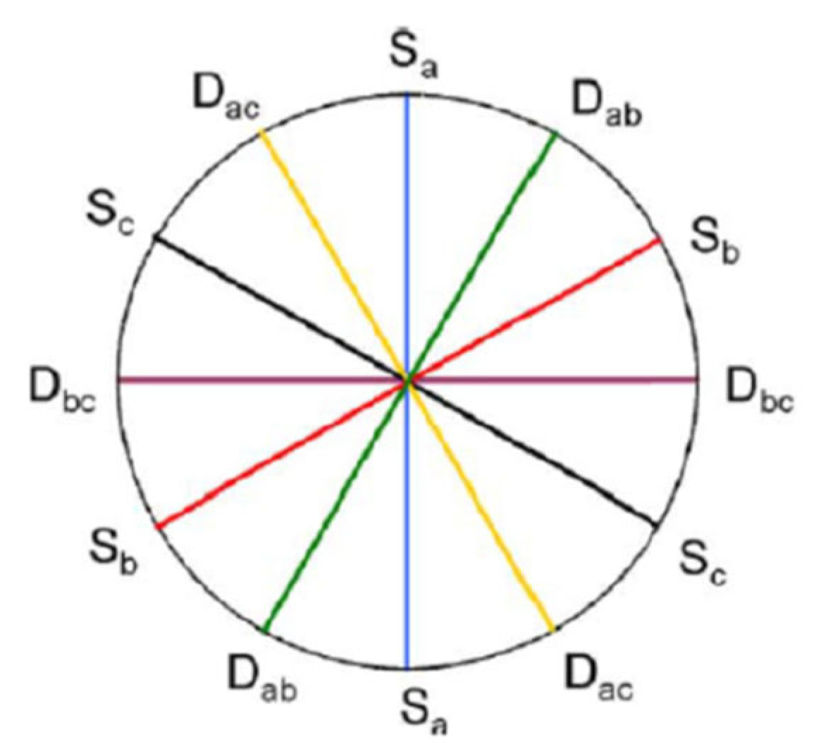
Clarke transformation is also the basis for the definition of voltage/current space vectors [15,16,17,18]. A voltage/current space vector is a complex-valued time function where the real and imaginary parts are given by the α and β components of a Clarke-transformed voltage/current, respectively. In the ideal unfaulted case, the trajectory of the voltage space vector on the complex plane is circular. On the contrary, in the case of an asymmetrical fault, the trajectory of the voltage space vector on the complex plane is elliptical, where the inclination angle of the ellipse allows the classification of the kind of fault [19,20,21,22,23,24,25,26,27,28,29,30]. Figure 1 shows the classification angles for single-phase (S) and double-phase (D) faults [30]. Notice that in [30], only the special case of a steady-state single-phase fault was considered. In this paper, however, the transient solution through the Clarke transformation is proposed, and a more general fault condition is considered, including asymmetrical double-phase faults. Thus, the results derived in the paper also allow straightforward detection, classification, and characterization of a specific kind of fault. Moreover, the impact of circuit parameters on the effectiveness of fault characterization can be readily determined.
The general methodology introduced in this paper can be outlined as follows. The main assumption is the three-phase symmetry of the system, apart from the fault section where fault constraints are typically asymmetrical. The symmetric part of the three-phase system is processed according to the Clarke transformation. Thus, three circuits, named α, β, and zero, with transformed topology and variables can be defined. The asymmetrical part, i.e., the fault section, is characterized by specific constraints on the phase variables, depending on the kind of fault (i.e., single/double-phase, grounded/ungrounded). The constraints on the phase variables, once Clarke transformed, become constraints on the α, β, and 0 variables at the fault location. Through specific mathematical derivations, it is shown that such constraints can be represented as proper circuit elements (mainly ideal transformers) coupling the α, β, and 0 circuits. Thanks to such simple equivalent circuits, the three-phase transient can be easily solved in the time domain for each specific kind of fault. It is worth highlighting that such an approach is not approximate, but it provides a rigorous and exact analytical solution, equivalent to the instantaneous SCT solution. Numerical simulations of transients in a three-phase radial system validate the correctness of the proposed analytical approach.
The paper is organized as follows. In Section 2, the instantaneous SCT is discussed. In Section 3, the Clarke transformation and some topological aspects are reported. In Section 4, the analytical derivations for the single-phase fault, the double-phase grounded/ungrounded faults, and the introduction of the related equivalent circuits are presented in detail. In Section 5, a comparison between the instantaneous SCT and Clarke equivalent circuits for transient analysis is presented. Numerical validation of the derived analytical results and equivalent circuits is reported in Section 6 for a three-phase radial system. Finally, conclusions are presented in Section 7.

2. Conventional Transient Analysis Through Instantaneous SCT

Transient analysis of three-phase systems was introduced in [10] with specific reference to rotating electric machines. The methodology, however, can be readily extended to general power systems as shown in [11]. The basic underlying idea consists of extending the conventional SCT, originally introduced in the phasor domain, to time-domain variables. Therefore, by considering a column vector of time-domain phase voltages v a b c = v a v b v c T , the instantaneous SCT (ISCT) is defined as:
v p n 0 = v ¯ p v ¯ n v 0 = S v a b c = 1 3 1 a a 2 0 a 2 a 1 1 1 v a v b v c
where S is the SCT matrix in the power invariant form such that S 1 = S * T , a = e j 2 π 3 , v ¯ p and v ¯ n are complex-valued voltages such that v ¯ n = v ¯ p * , whereas v 0 is a real-valued voltage. Of course, the same transformation given in (1) holds for phase currents.
Notice that since the ISCT (1) is based on the same transformation matrix S as the conventional SCT, asymmetrical-fault transient analysis leads to the same equivalent circuits commonly used for the steady-state analysis of asymmetrical faults. This point will be detailed in Section 5 where the ISCT approach will be compared with the Clarke components approach proposed in this paper.

3. Clarke Transformation and Three-Phase Circuit Analysis

Let us consider a column vector of time-domain phase voltages v a b c . The Clarke transformation of v a b c is defined as [4,5,6]:
v α β 0 = v α v β v 0 = T v a b c = 2 3 1 1 2 1 2 0 3 2 3 2 1 2 1 2 1 2 v a v b v c
where the transformation matrix T is defined in the power invariant form, from the abc domain to the transformed α β 0 domain. This property is of paramount importance in order to define consistent equivalent circuits in the Clarke domain.
The main feature of the Clarke transformation is the diagonalization of balanced three-phase component matrices. As a remarkable example, for a symmetrical mutual inductor in the time domain, we obtain [30]:
v α v β v 0 = T L p h L m L m L m L p h L m L m L m L p h T 1 d d t i α i β i 0 = = L p h L m 0 0 0 L p h L m 0 0 0 L p h + 2 L m d d t i α i β i 0 = = L α 0 0 0 L β 0 0 0 L 0 d d t i α i β i 0
Thus, three uncoupled equations were obtained in (3). Moreover, by considering that L α = L β , the first two equations can be combined in one complex equation as:
v ¯ = v α + j v β = L d d t i α + j i β = L d d t i ¯
where the voltage/current space vectors v ¯ and i ¯ have been introduced.
In case of a three-phase sinusoidal voltage source with phase voltages e = e a e b e c T , by using the Clarke transformation, we obtain the following space vector:
e ¯ = e α + j e β = E p e j ω t + E n * e j ω t
where E p and E n are the positive/negative sequence components provided by the phasor SCT [29,30]:
E S = E p E n E 0 = S E = 1 3 1 a a 2 1 a 2 a 1 1 1 E a E b E c
Under sinusoidal steady state, the trajectory of the space vector e ¯ is elliptical, and the semi-major axis r M , the semi-minor axis r m , and inclination angle φ , are given by [29,30]:
r M = E p + E n * ,             r m = E p E n *
φ = 1 2 a r g E p + a r g E n *
Clarke equivalent circuits in the α β 0 variables can be obtained by transforming three-phase components as in (2) and by transforming three-phase symmetrical connections. The most common three-phase connections are the star connections, where the star center can be either non-accessible or accessible to connect the three-phase system to single-phase networks [30].

3.1. Star Connection with Non-Accessible Center

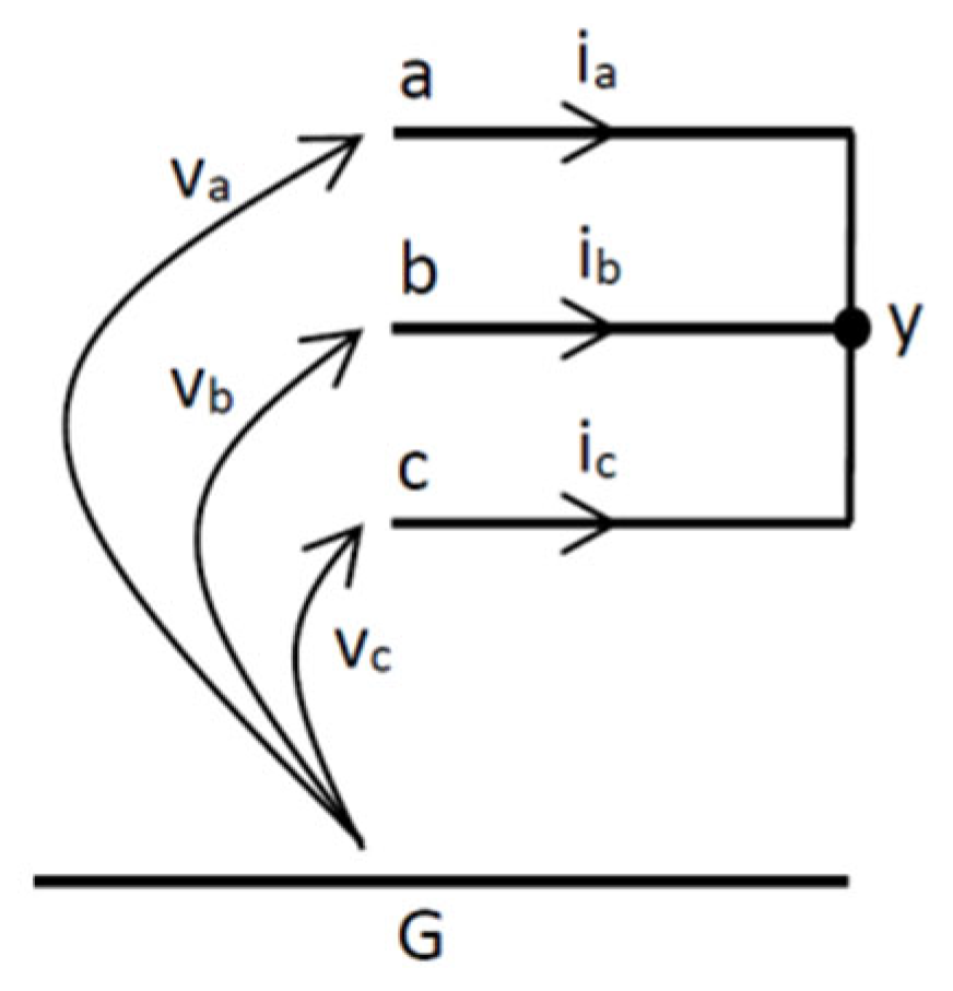
Figure 2 shows a star connection with a non-accessible star center. By assuming a reference terminal G valid for the whole three-phase system, the star connection can be considered a three-port network characterized by the following independent relationships:
v a = v b ,             v b = v c ,             i a + i b + i c = 0
By using (9) in the Clarke transformation (2), we obtain:
v α = v β = 0
i 0 = 0
i.e., the star connection with a non-accessible center is equivalent to a short circuit in the α β domains and an open circuit in the 0 domain.

3.2. Star Connection with Accessible Center

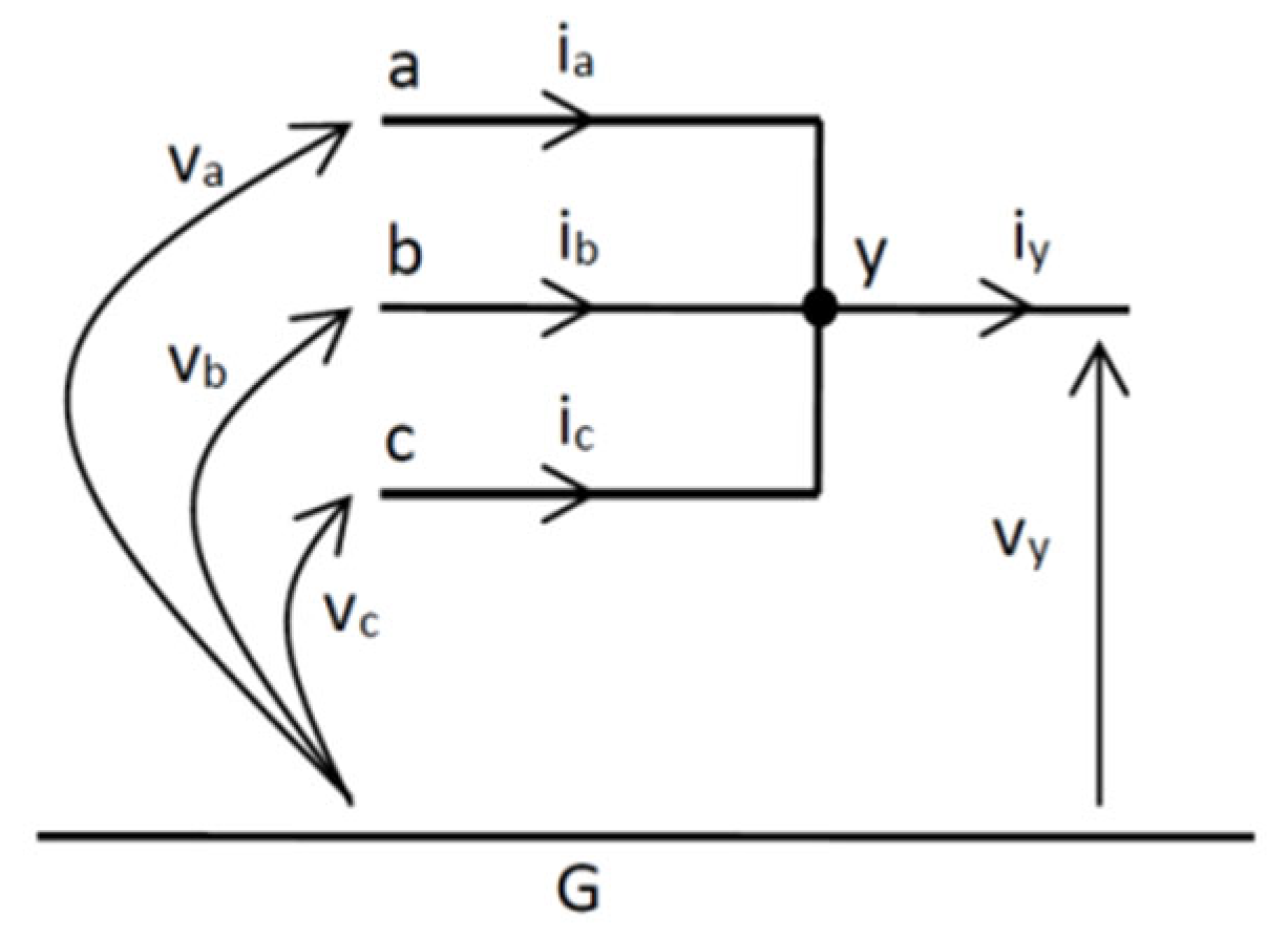
Figure 3 shows a star connection with an accessible star center. The star center is normally used to connect the three-phase system to a single-phase circuit. This connection can be treated as a four-port network whose independent relationships are given by:
v a = v y ,         v b = v y ,         v c = v y ,         i a + i b + i c = i y
By using (12) in the Clarke transformation (2), we obtain that this kind of connection is a short circuit in the α β domains, whereas in the 0 domain:
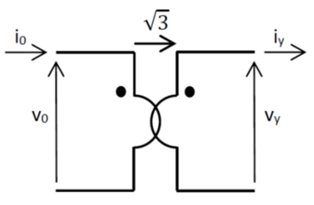
v 0 = 3 v y
i 0 = 1 3 i y
i.e., the interconnection between the 0 (three-phase) domain and the single-phase domain can be represented as an ideal transformer with a turn ratio 3 (see Figure 4). The well-known properties of ideal transformers can be readily used to analyze circuits in the 0 domain and the interconnections with single-phase circuits.

4. Clarke Transient Analysis of Asymmetrical Faults

In this section, the time-domain analysis of asymmetrical faults based on the Clarke transformation recalled in Section 3 will be developed. In particular, the following faults will be considered: (a) single-phase faults, (b) double-phase grounded faults, (c) double-phase ungrounded faults.
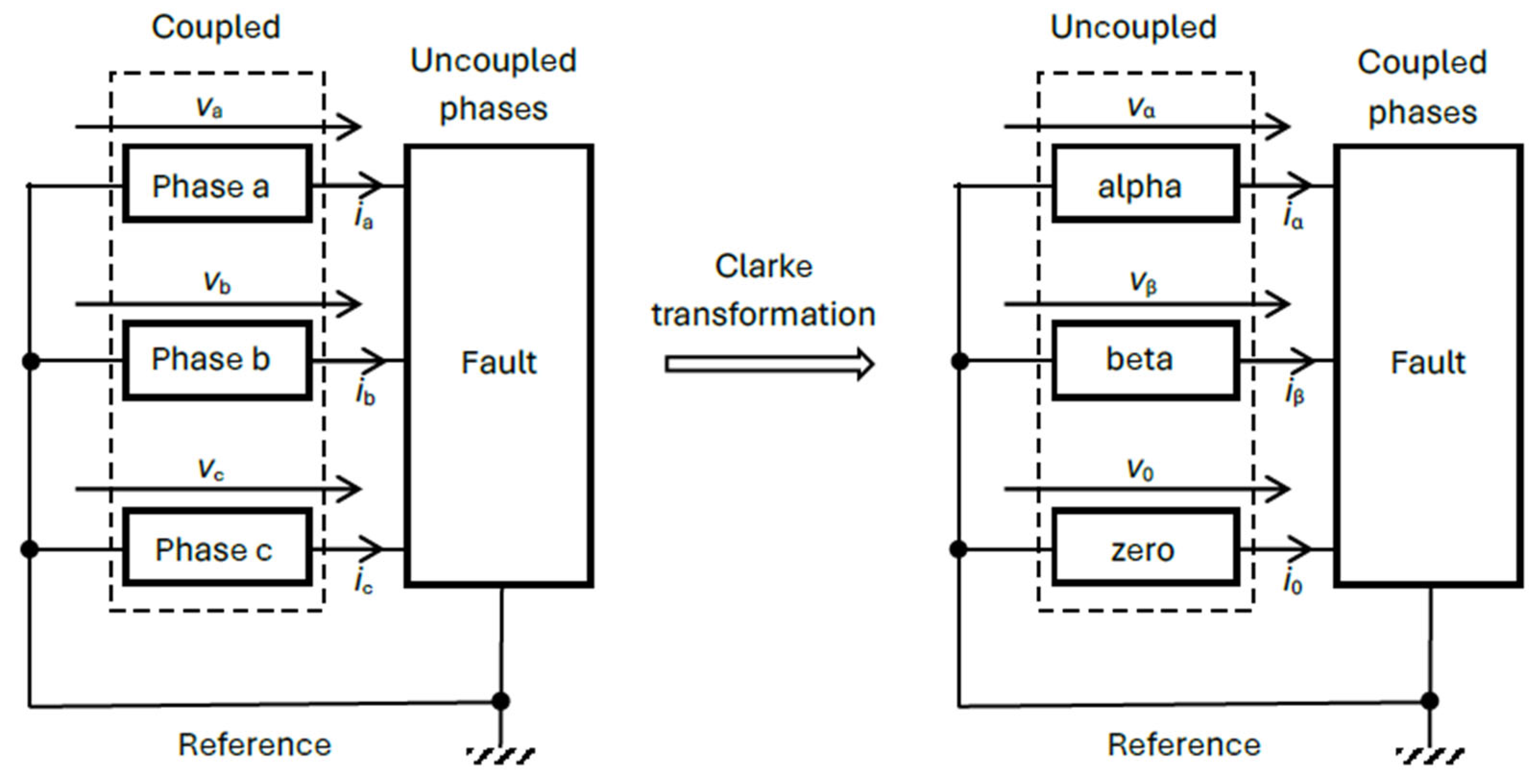
Figure 5 shows the effect of Clarke transformation on the circuit variables. In the abc domain, phase voltages and currents belonging to the symmetrical part of the three-phase circuit are coupled, whereas the asymmetrical fault can usually be represented as uncoupled phase constraints. On the contrary, after Clarke transformation, the αβ0 variables in the symmetrical portion of the three-phase circuit are uncoupled, whereas the asymmetrical fault constraints result in coupled αβ0 variables. Thus, the αβ0 circuits result in coupled circuits at the fault location only. The effect of the Clarke transformation is, therefore, to move the circuit coupling from the whole three-phase system (i.e., the left side in Figure 5) to the asymmetrical fault only (i.e., the right side in Figure 5).

4.1. Single-Phase Faults

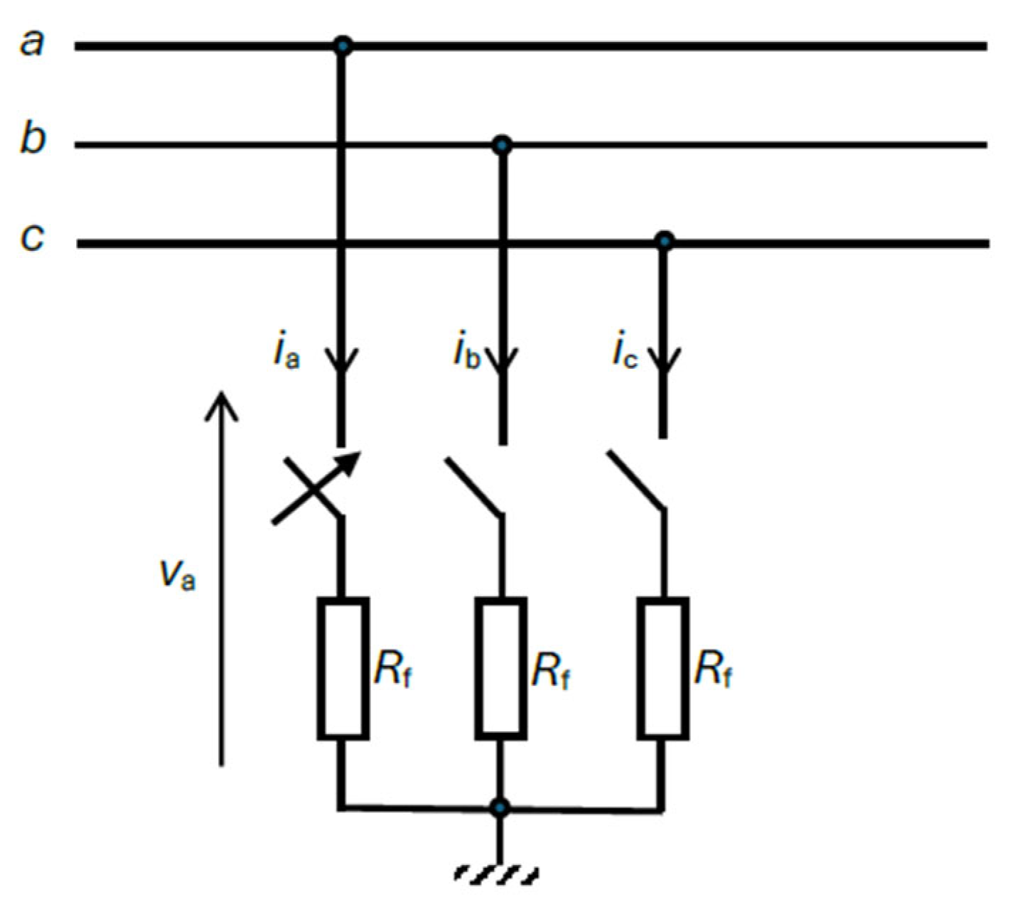
A single-phase fault can be represented as in Figure 6, where only the switch corresponding to the faulted phase is closed. For the sake of simplicity, we assume a resistive fault R f ; however, a generic RLC fault could be considered in the proposed time-domain analysis.
By assuming that the faulted phase is phase a, the corresponding fault constraints on the phase variables are given by:
v a = R f i a ,   i b = i c = 0
By using (15) in the Clarke transformation defined in (2), we can readily obtain the αβ0 voltages and currents:
v α β 0 = v α v β v 0 = 2 3 1 1 2 1 2 0 3 2 3 2 1 2 1 2 1 2 R f i a v b v c = 2 3 R f i a v b + v c 2 3 v b v c 2 R f i a + v b + v c 2
i α β 0 = i α i β i 0 = 2 3 1 1 2 1 2 0 3 2 3 2 1 2 1 2 1 2 i a 0 0 = 2 3 i a 0 1 2 i a
From (17), we observe that i β = 0 , i.e., β is an open circuit. Moreover:
i 0 = 1 2 i α
By taking into account (17) in (16), for the α and 0 circuits, we obtain:
v α = R f i α v b + v c 6
v 0 = R f i 0 + v b + v c 3
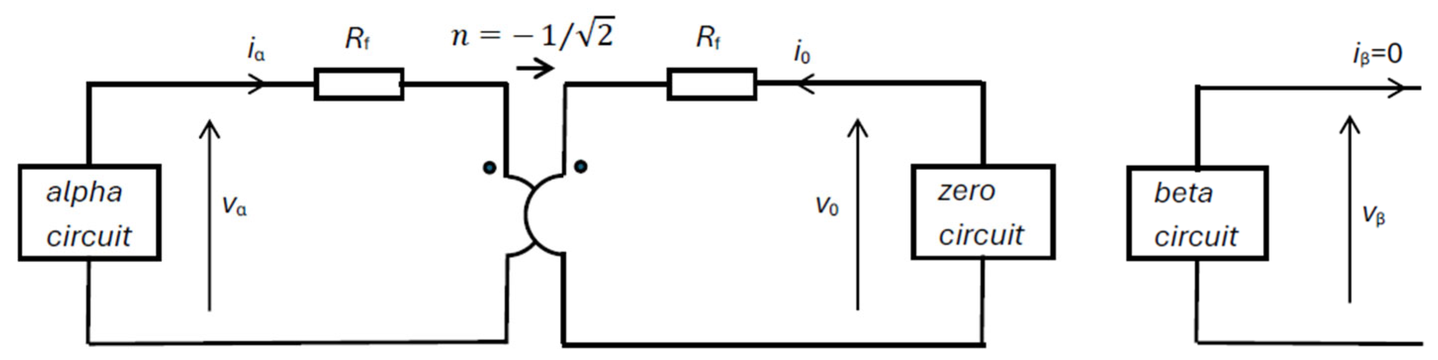
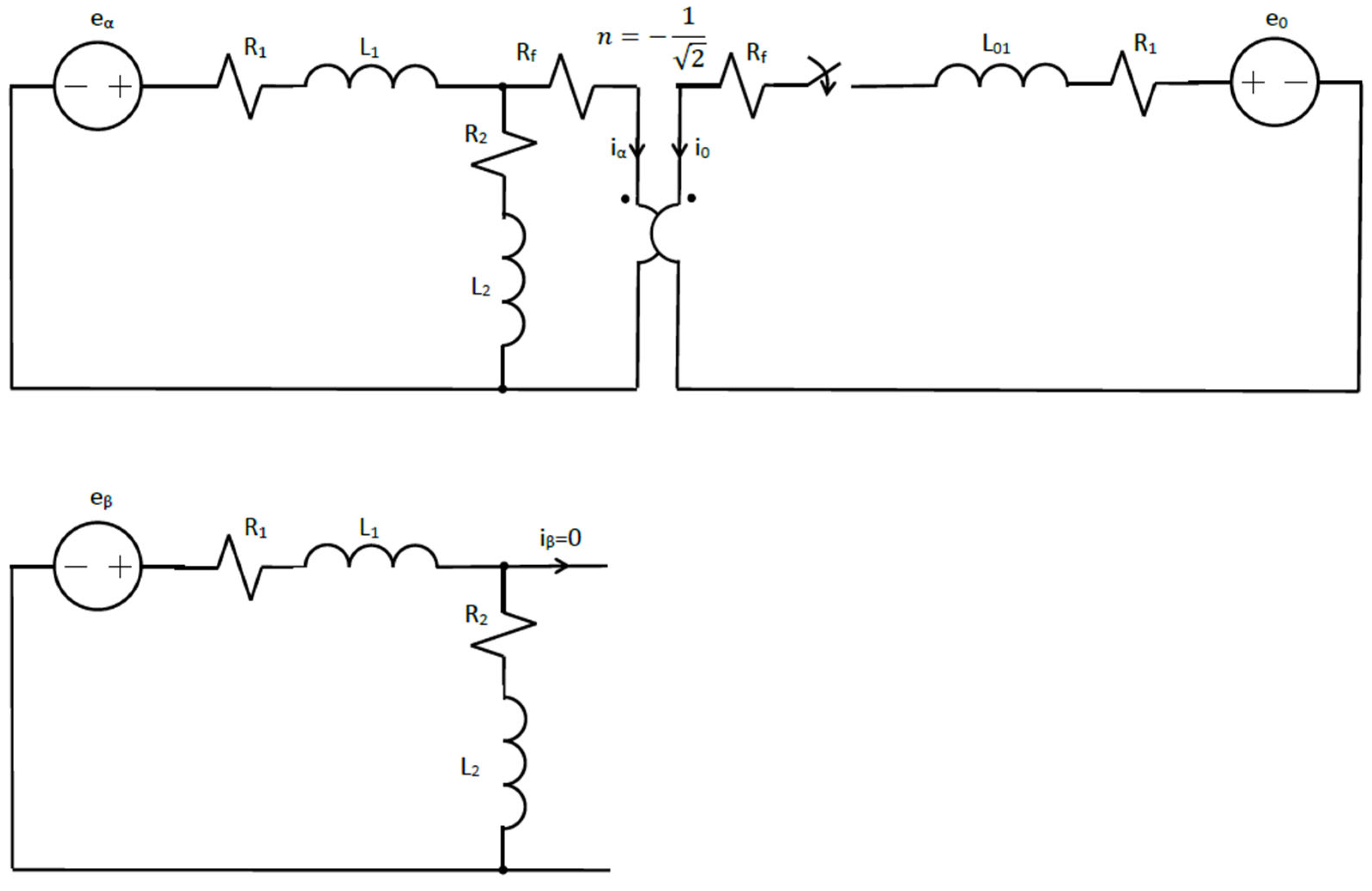
Thus, from (18)–(20) we can readily obtain the circuit representation of coupling between α and 0 circuits through an ideal transformer with a turn ratio n = 1 / 2 as in Figure 7, where the open β circuit is also represented.
Notice that, according to the space vector definition (4), the β component of the voltage is not affected by the fault, whereas the transient of the α component is affected by the coupling with the 0 circuit. As far as the current space vector is considered, we can observe that its β component is zero. Thus, the current transient is fully described by the α component of the current space vector, affected by the coupling with the 0 circuit.
Finally, once the αβ0 circuits in Figure 7 are solved, the phase abc variables at the fault location can be recovered through the inverse Clarke transformation. As far as the voltages are concerned, we obtain:
v a b c = v a v b v c = 2 3 1 0 1 2 1 2 3 2 1 2 1 2 3 2 1 2 v α v β v 0 = 2 3 R e v ¯ + 1 2 v 0 R e a 2 v ¯ + 1 2 v 0 R e a v ¯ + 1 2 v 0
where v ¯ is the space vector defined in (4), and R e · takes the real part.
As far as the abc currents are considered, in this case, only i a is different from zero. From (17), we readily obtain:
i a = 3 2 i α = 3 i 0

4.2. Double-Phase Grounded Faults

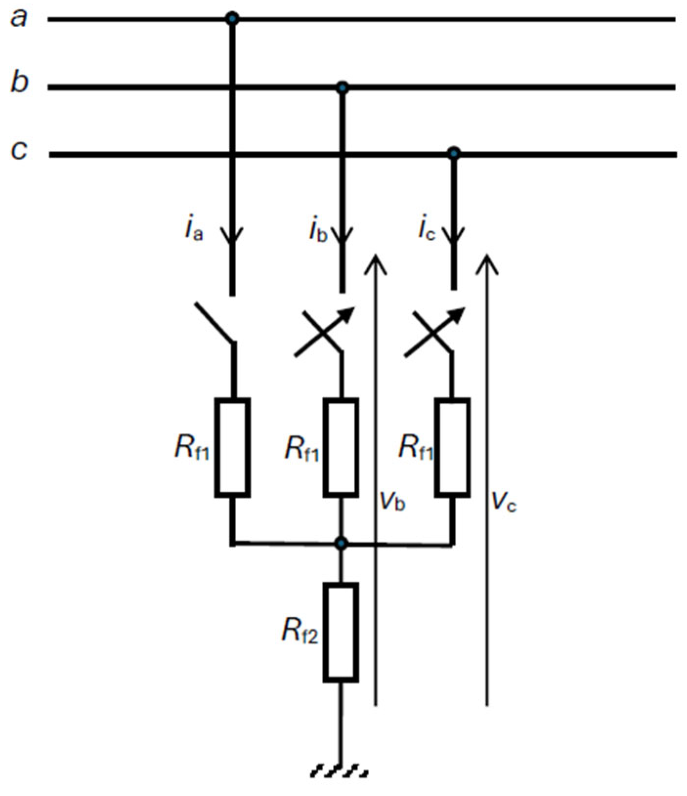
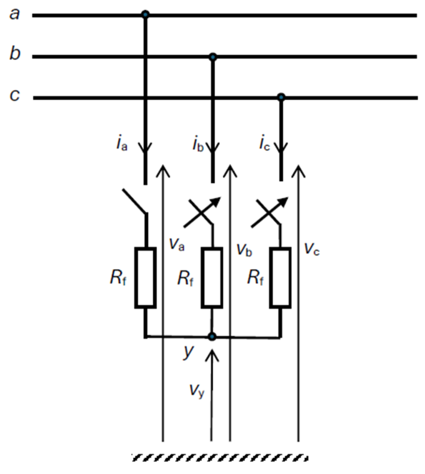
Double-phase grounded faults involve two phases and the ground. In the general case, a double-phase fault can be represented as in Figure 8, where only two switches are closed. By closing the switches b and c, the corresponding constraints on the phase variables are given by:
i a = 0 ,   v b = R f 1 i b + R f 2 i b + i c ,   v c = R f 1 i c + R f 2 i b + i c
By using (23) in the Clarke transformation defined in (2), we can readily obtain the αβ0 voltages and currents:
v α β 0 = v α v β v 0 = 2 3 1 1 2 1 2 0 3 2 3 2 1 2 1 2 1 2 v a R f 1 i b + R f 2 i b + i c R f 1 i c + R f 2 i b + i c = = 2 3 v a 1 2 R f 1 + 2 R f 2 i b + i c 3 2 R f 1 i b i c 1 2 v a + R f 1 + 2 R f 2 i b + i c
i α β 0 = i α i β i 0 = 2 3 1 1 2 1 2 0 3 2 3 2 1 2 1 2 1 2 0 i b i c = 2 3 1 2 i b + i c 3 2 i b i c 1 2 i b + i c
From (24) and (25), using simple algebra, we obtain:
i 0 = 2 i α
and
v α = 2 3 v a + R f 1 + 2 R f 2 i α
v β = R f 1 i β
v 0 = 1 3 v a + R f 1 + 2 R f 2 i 0
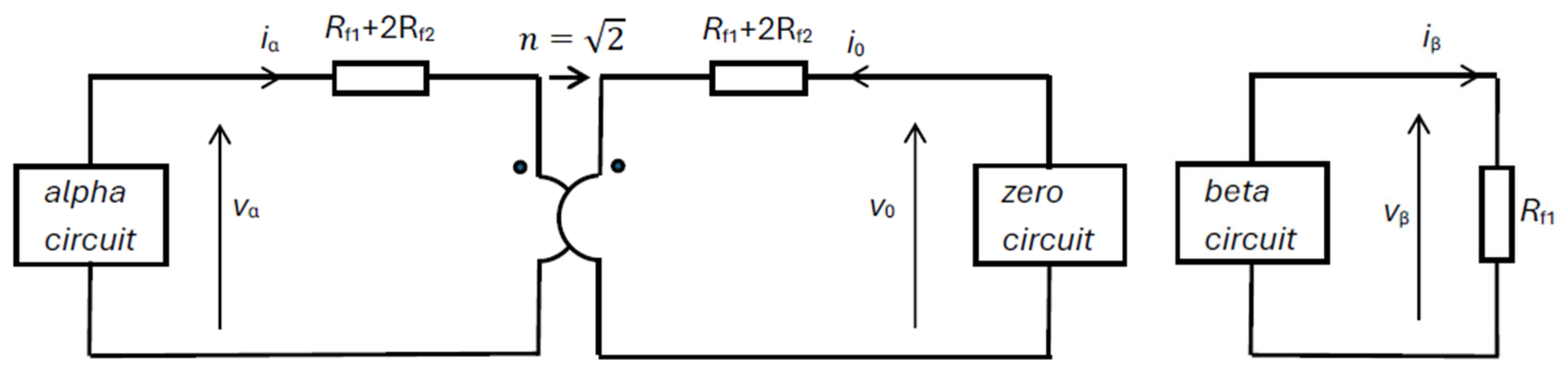
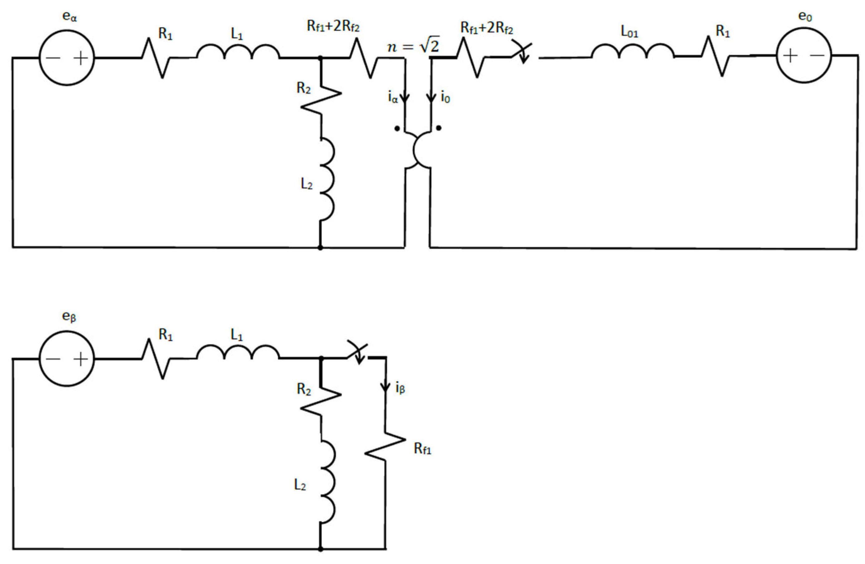
Therefore, the α and 0 circuits can be represented as coupled circuits through an ideal transformer with a turn ratio n = 2 , whereas the β circuit is uncoupled and loaded with the fault resistor R f 1 (see Figure 9).
Notice that in this case, the transient involves all three components αβ0. Moreover, fault grounding results in circuit coupling between α and 0 circuits.

4.3. Double-Phase Ungrounded Faults

In the special case of an ungrounded double-phase fault, the fault resistor R f 2 in Figure 8 is replaced by an open circuit (see Figure 10).
By taking into account the current constraint i a = i y = 0 , we can write:
i c = i b
Thus, the phase voltages in this case are given by:
v a = v a y + v y
v b = v b y + v y = R f i b + v y
v c = v c y + v y = R f i b + v y
By using (30) and (31) in the Clarke transformation defined in (1), we can readily obtain the αβ0 voltages and currents:
v α β 0 = v α v β v 0 = 2 3 1 1 2 1 2 0 3 2 3 2 1 2 1 2 1 2 v a y + v y R f i b + v y R f i b + v y = 2 3 v a y 3 R f i b 1 2 v a y + 3 v y
i α β 0 = i α i β i 0 = 2 3 1 1 2 1 2 0 3 2 3 2 1 2 1 2 1 2 0 i b i b = 2 3 0 3 i b 0
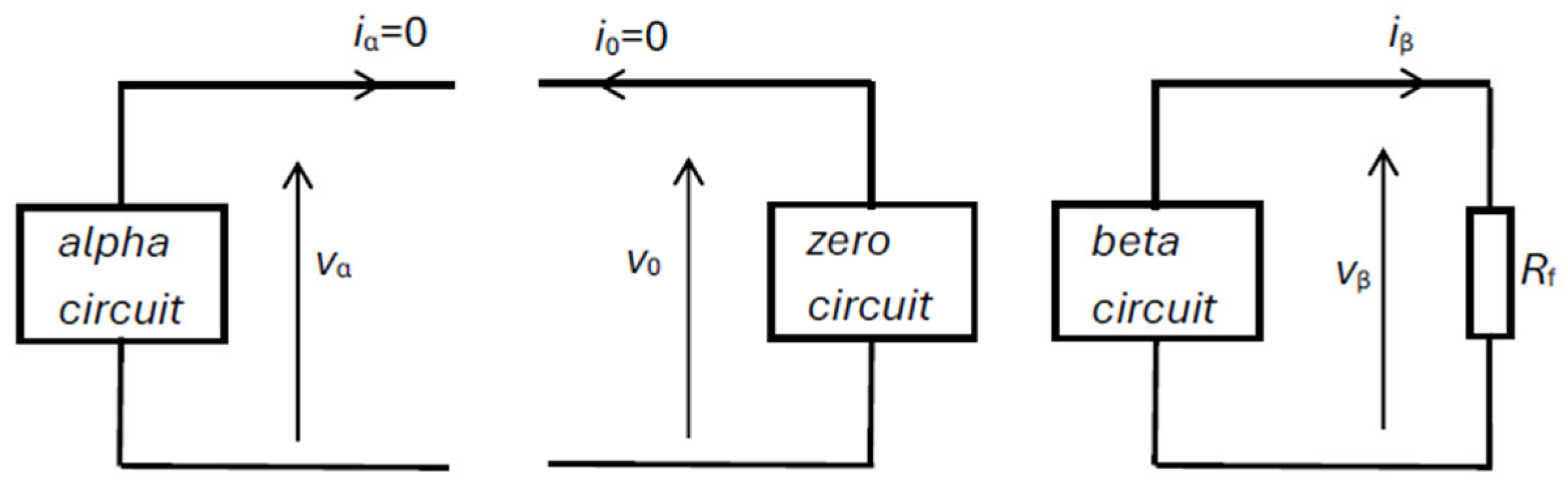
Notice that v α and v β are not dependent on v y . Moreover, since i α = i 0 = 0 , the α and 0 circuits are open circuits, whereas the β circuit is closed on the fault resistor R f , such that (see Figure 11):
v β = R f i β
as in the grounded fault case (28). Thus, in the ungrounded double-phase fault, the transient involves only the β circuit. This is the opposite behavior of the single-phase fault described in Section 4.1. The α and 0 circuits remain in the steady-state open-circuit condition; therefore, they can be readily solved as transient-free circuits.
Once i β is calculated by solving the transient β circuit, i b can be recovered from (33) as i b = i β / 2 . Moreover, the phase voltages can be recovered from the inverse Clarke transformation (21).

5. Comparison Between Clarke and ISCT Transient Analysis

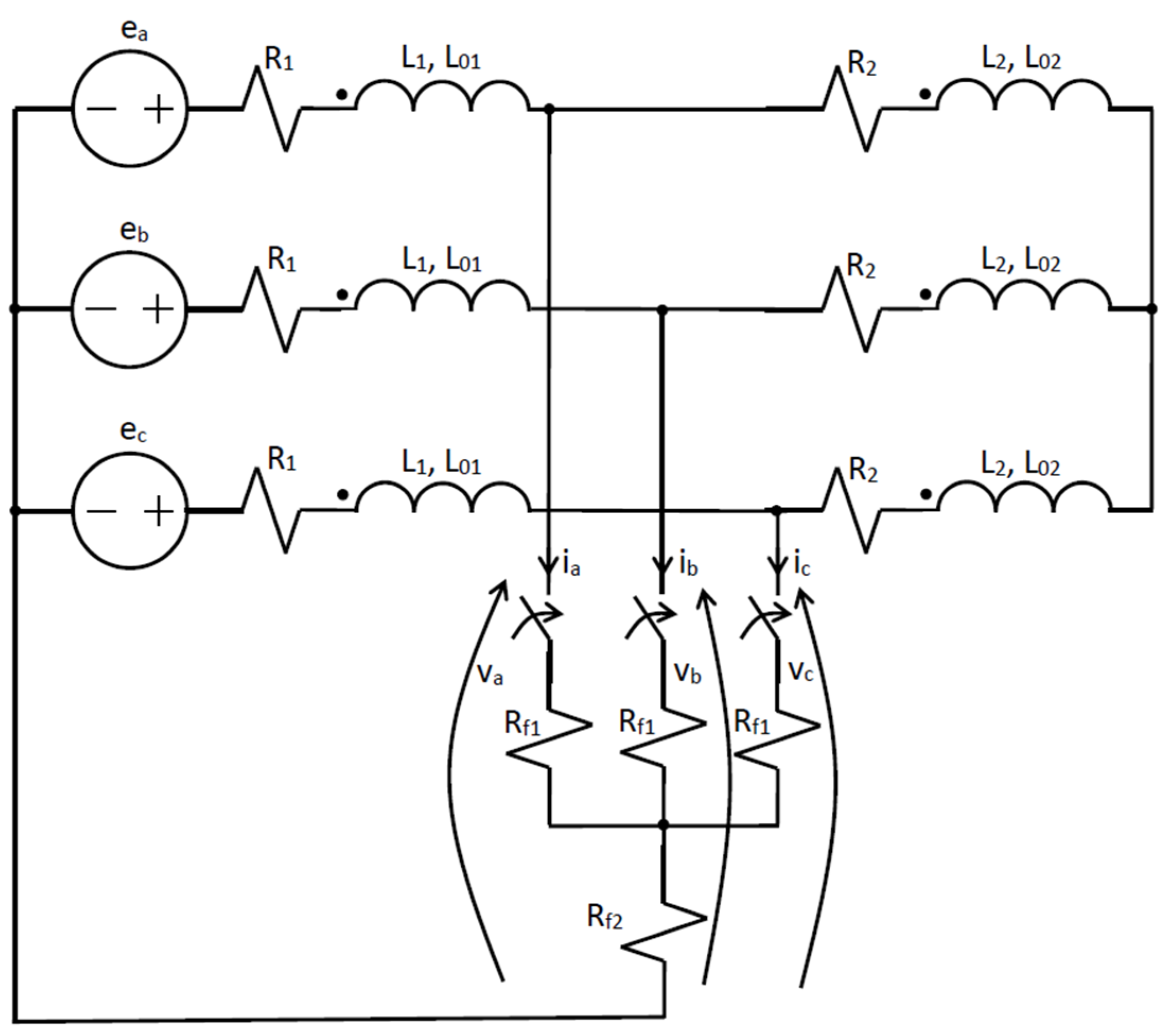
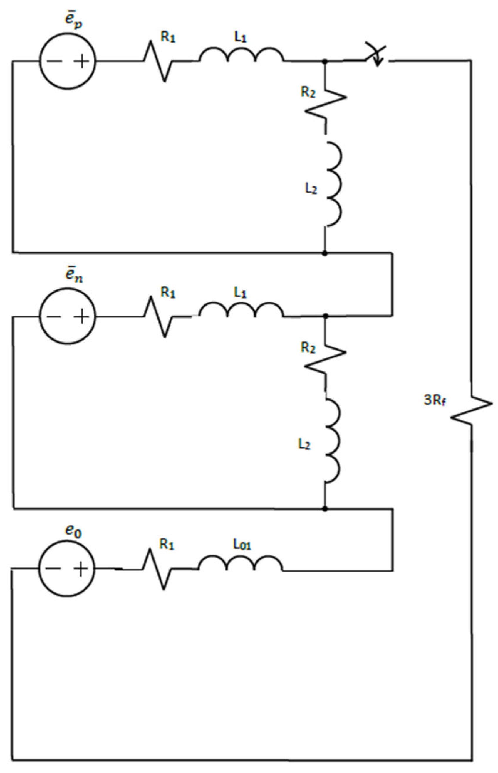
Transient analyses by adopting Clarke and ISCT approaches will be compared using the three-phase system depicted in Figure 12. It will be shown that since the Clarke approach provides equivalent circuits where the α, β, and 0 components are not all coupled, the dynamic order of each equivalent circuit is lower than the equivalent circuit corresponding to the ISCT approach. Equivalent circuits with reduced dynamic order require simpler calculations in both numerical and analytical/hand approaches.
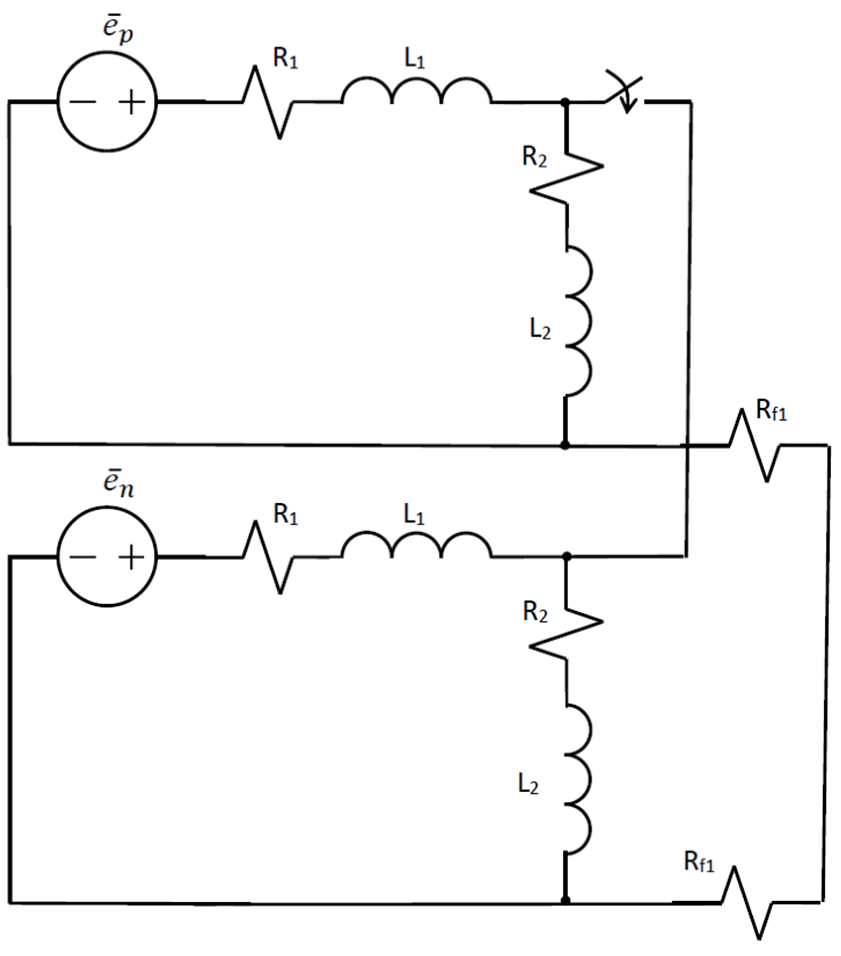
As far as the single-phase fault is concerned, i.e., only switch a in Figure 12 is operated, the ISCT provides the equivalent circuit in Figure 13 where R f = R f 1 + R f 2 , and the three sequence circuits are connected in series. Notice that the circuit in Figure 13 is a third-order dynamic circuit. In fact, despite the number of inductors being five, the number of independent inductors is three.
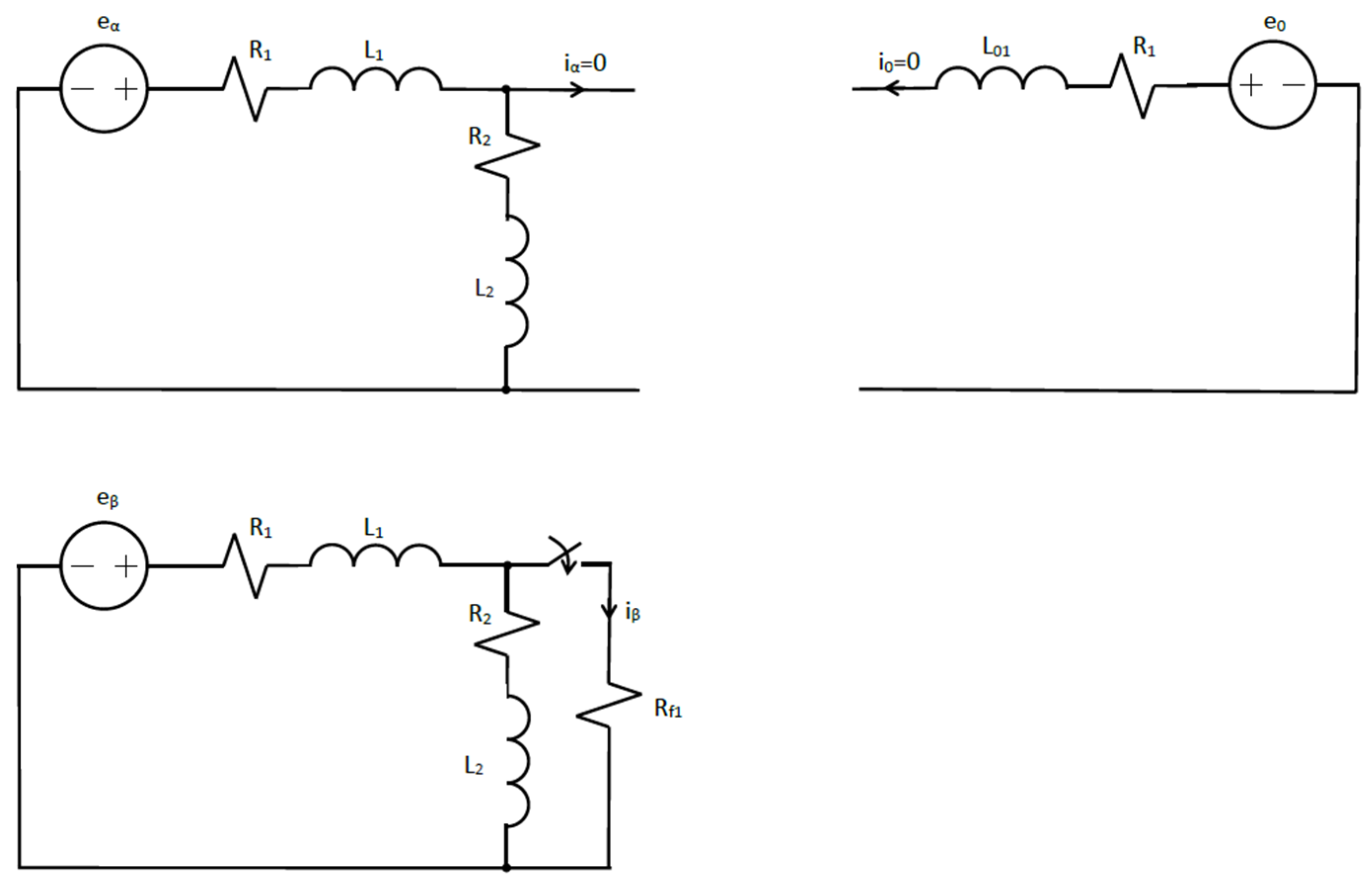
In Figure 14, the Clarke equivalent circuits corresponding to Figure 7 are shown. It is apparent that the β circuit is independent of the α and 0 circuits. Actually, the α-0 circuit is a second-order dynamic circuit, whereas the β circuit is a first-order circuit, such that the whole dynamic order remains equal to three. Moreover, notice that the β circuit has no transients; thus, it requires the steady-state solution only. Therefore, by adopting the Clarke approach, a second-order dynamic circuit must be solved instead of a third-order circuit as in the ISCT approach.
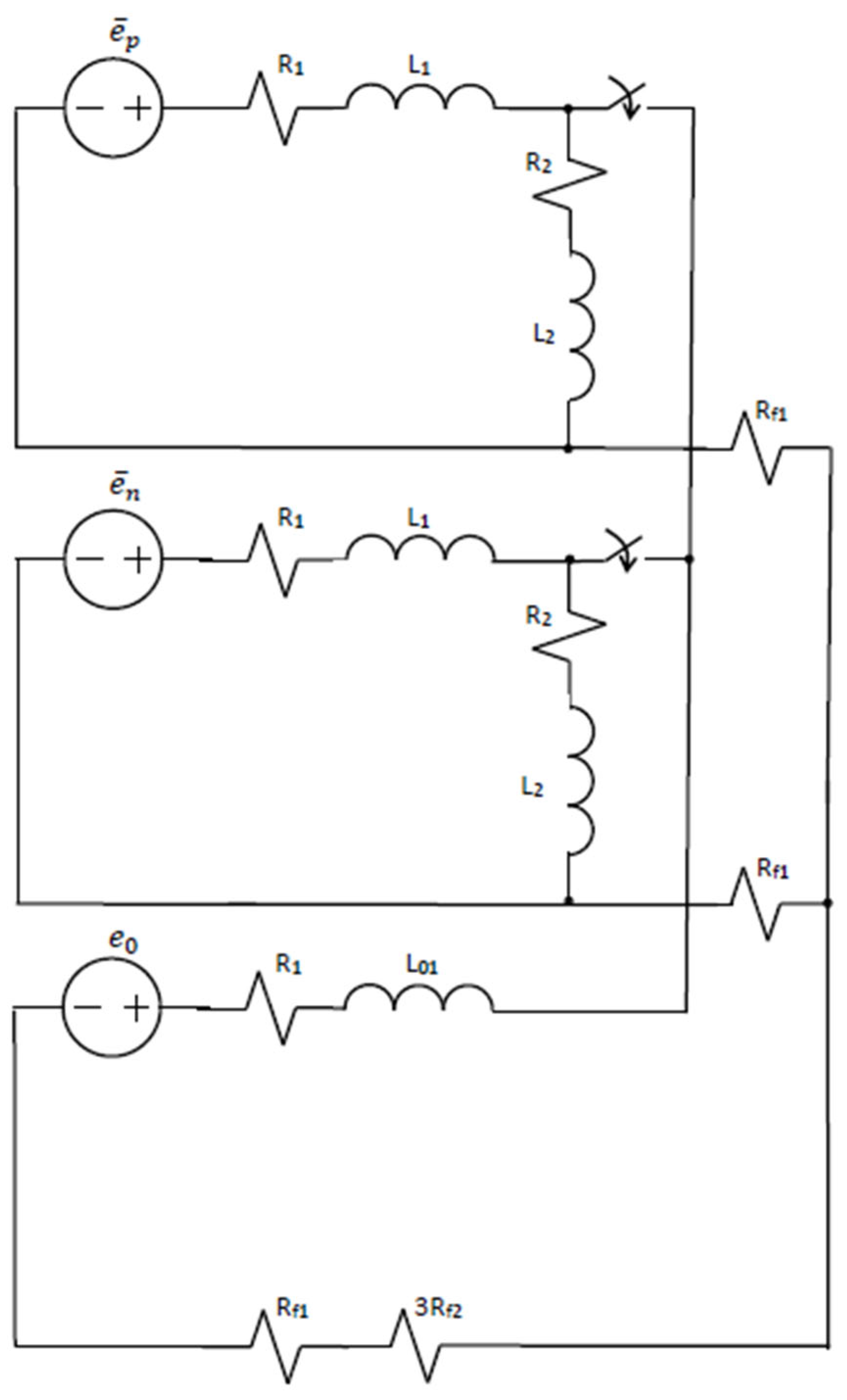
As far as the double-phase grounded fault is concerned, the ISCT approach provides the equivalent circuit represented in Figure 15, where the three sequence circuits are connected in parallel. The effective dynamic order of the circuit, i.e., the number of independent inductors, is four. Figure 16 shows the equivalent circuits provided by the Clarke approach corresponding to Figure 9. Notice that in this case, the β circuit is independent of the α-0 circuit. Moreover, both the Clarke circuits are second-order dynamic circuits. Thus, the whole dynamic order remains equal to four, but the two independent circuits provided by the Clarke approach require simpler calculations because each of them is a second-order circuit whose solution can be readily obtained by hand calculations.
As far as the double-phase ungrounded fault is concerned, the ISCT provides the equivalent circuit represented in Figure 17. Notice that it can be derived from Figure 15 by letting R f 2 . The circuit in Figure 17 is a third-order dynamic circuit. Figure 18 shows the equivalent circuits obtained from the Clarke approach, corresponding to Figure 11. The three Clarke circuits are independent. Moreover, the α circuit is in steady state, whereas the 0 circuit is an open circuit. The transient is represented only by the β circuit, which is a second-order dynamic circuit.

6. Numerical Validation

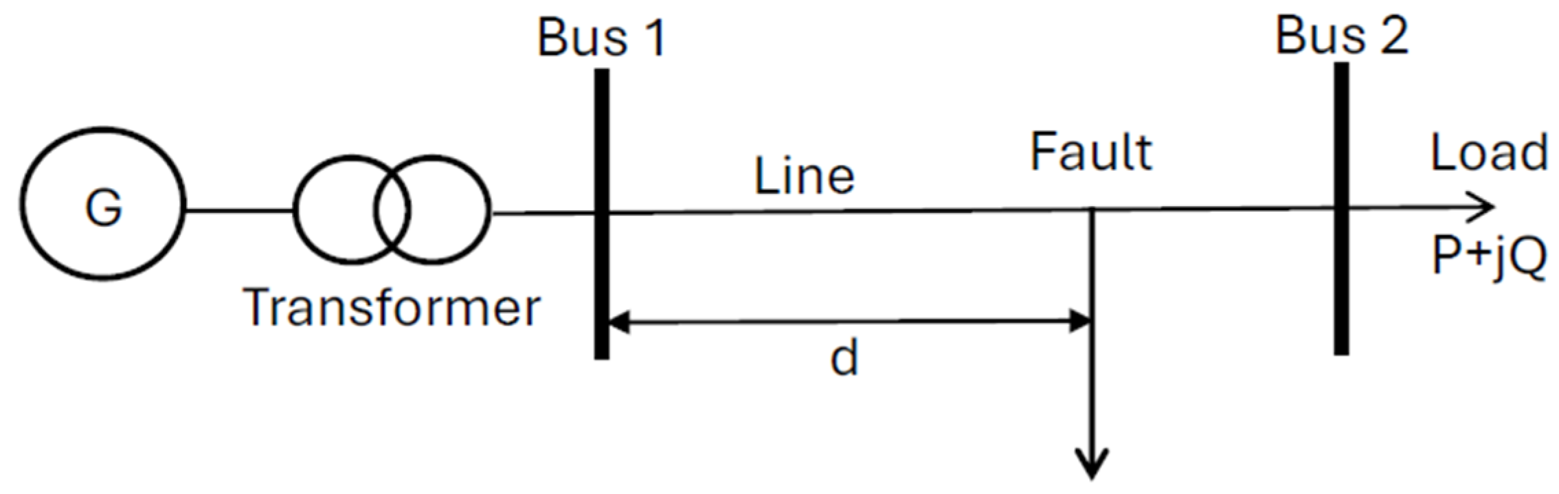
The analytical results derived in Section 4 were validated through numerical simulation in Matlab/Simscape R2025b of the simple radial system depicted in Figure 19.
The equivalent balanced generator is characterized by a 60 Hz phase voltage equal to 1 / 2   kV, positive/negative reactance X g = 0.5 Ω and resistance R g = 0.1 Ω, zero sequence reactance X 0 g = 0.25 Ω, and grounding reactance X g r = 0.2 Ω (see Table 1). The transformer, with a unity turn ratio, has a series positive/negative reactance X T = 0.1 Ω and zero sequence reactance X T 0 = 0.05 Ω. The line is modeled with positive/negative sequence reactance X l i n e = 0.3 Ω/km and resistance R l i n e = 0.1 Ω/km, and zero sequence reactance X 0 l i n e = 0.9 Ω/km. The fault is located at a distance d from bus 1.
The three fault cases analyzed in Section 4 were implemented by assuming fault locations d and fault resistance R f as parameters. For each case, the transient currents at the fault location and the locus of the voltage space vector at bus 1 were evaluated and plotted. Analytical and numerical results have always overlapped; therefore, in the following figures, no distinction has been made between analytical and numerical curves. Moreover, load effects were also negligible. Actually, in the existing literature, fault conditions are studied by neglecting the load [11,14,22].

6.1. Single-Phase Faults

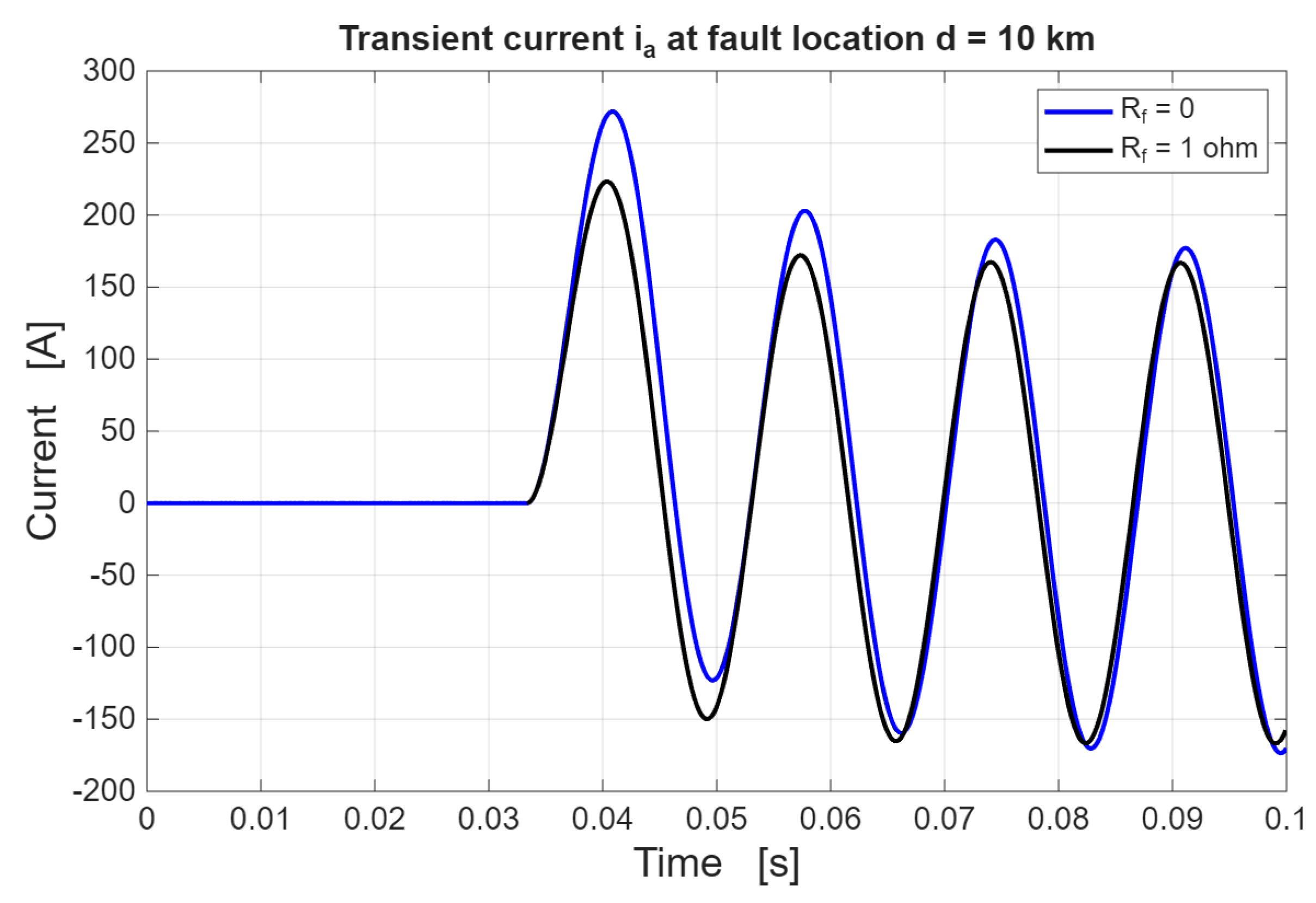
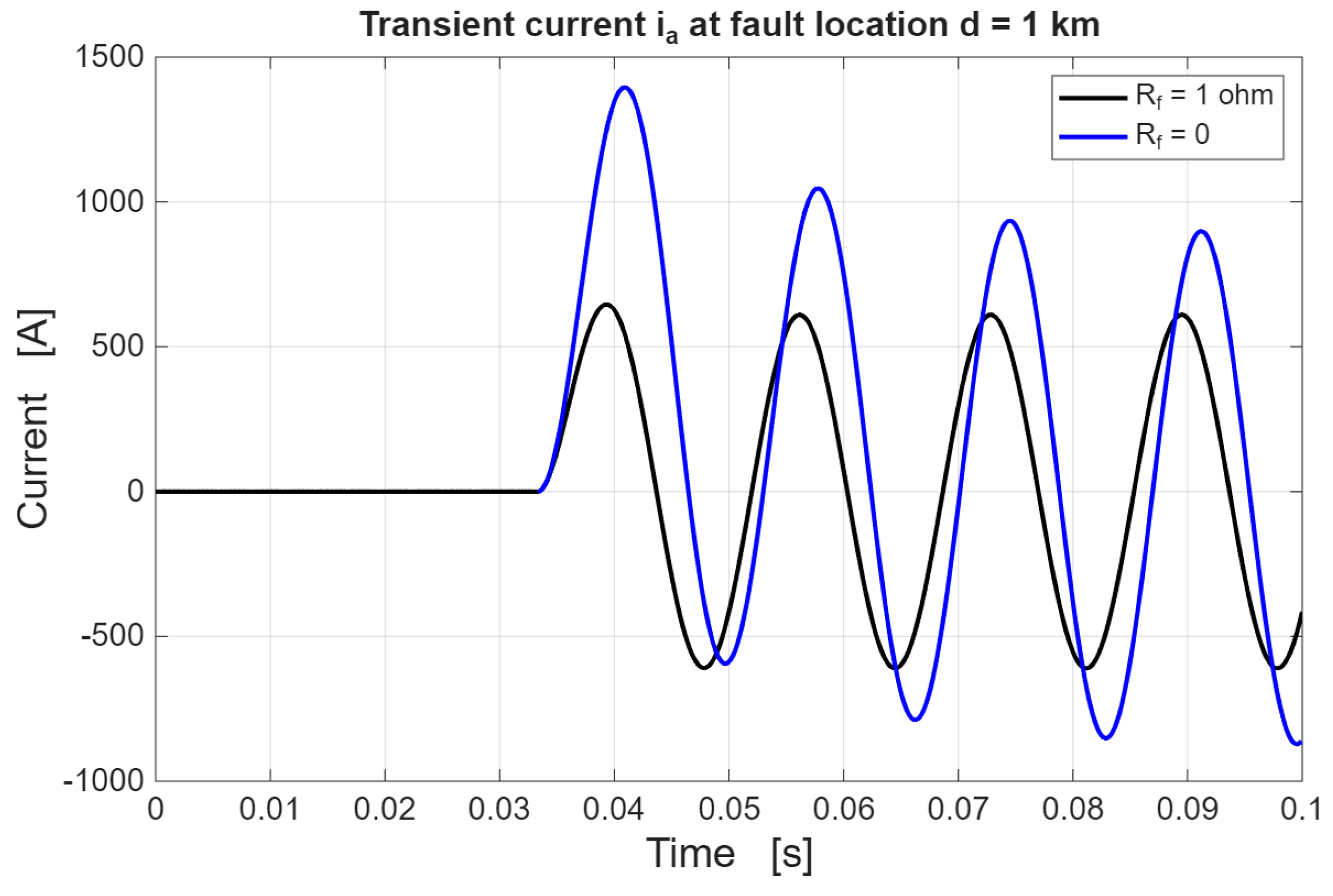
Single-phase faults, described in Section 4.1, have been implemented in Matlab/Simscape in order to validate the analytical results. In particular, the current i α and the corresponding fault current i a were evaluated at a fault location d = 10   km for two different values of fault resistance, i.e., R f = 0 and R f = 1   (see Figure 20). Clearly, a lower value of R f results in a larger excursion of the fault current and a larger time constant. This behavior is more evident in Figure 21, where the fault location is d = 1   km. Indeed, in this case, the line parameters have a lower impact, and therefore, the fault current has a larger excursion in the case of a fault with zero resistance.
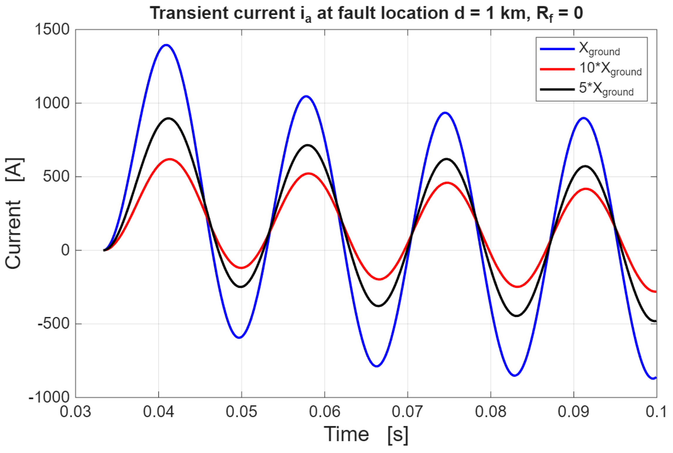
Figure 22 shows the behavior of the transient fault current i a for different values of the generator ground reactance X g r . Clearly, as expected, by increasing the ground reactance, the fault current decreases.
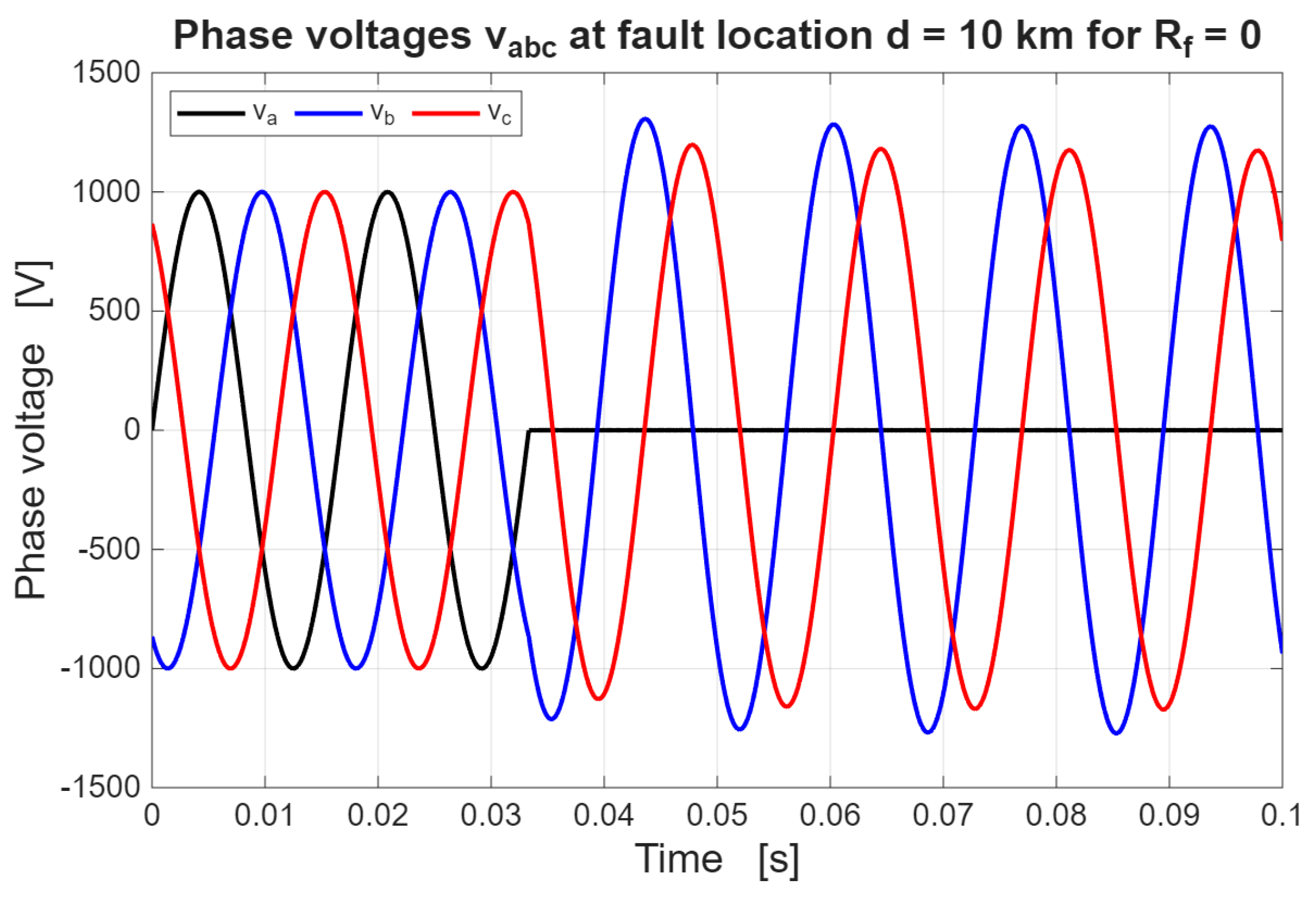
Figure 23 shows the phase voltages v a b c at a fault location d = 10   km for fault resistance R f = 0 . Overvoltage of unfaulted phases b and c is evident.
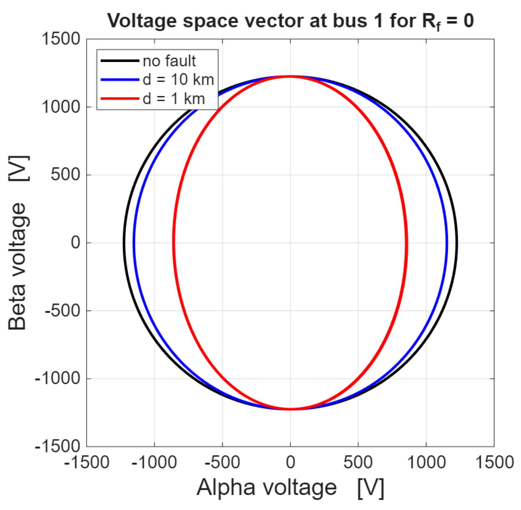
Figure 24 shows the behavior of the voltage space vector at bus 1 in the case of a fault with R f = 0 . The black curve shows the circular ideal trajectory in the case of no fault. The blue curve shows the trajectory in the case of a fault location d = 10   km, whereas the red curve shows the trajectory in the case of a fault location d = 1   km. Clearly, at a smaller distance, the detection of the single-phase fault becomes more evident, since the elliptical trajectory with inclination angle 90° can be readily detected. Figure 25 shows the voltage space vector in the case of a fault with R f = 1   . Notice that the fault resistance results in a slight deviation of the ellipse inclination and a smaller difference between d = 1   km and d = 10   km. Thus, as was expected, faults with larger resistance result in lower detection capability of the space vector trajectory. The apparent double red curve is due to the transient behavior.

6.2. Double-Phase Grounded Faults

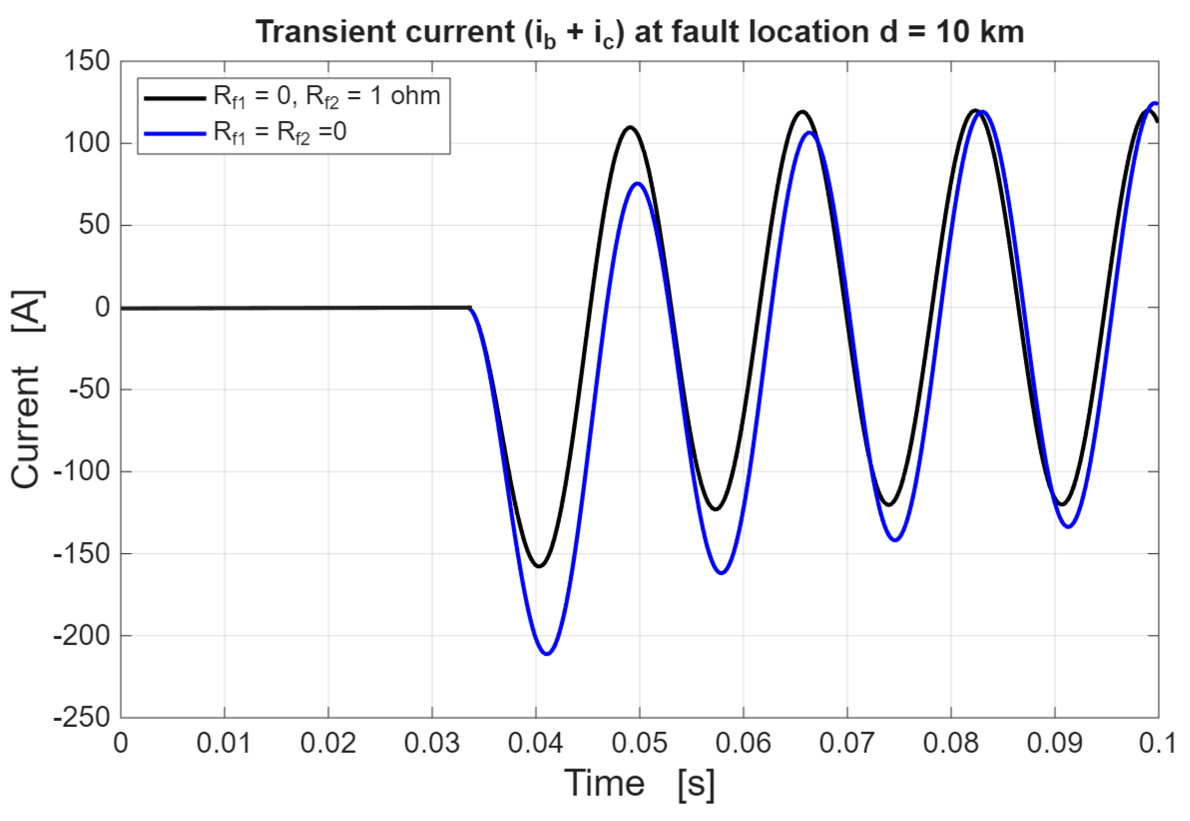
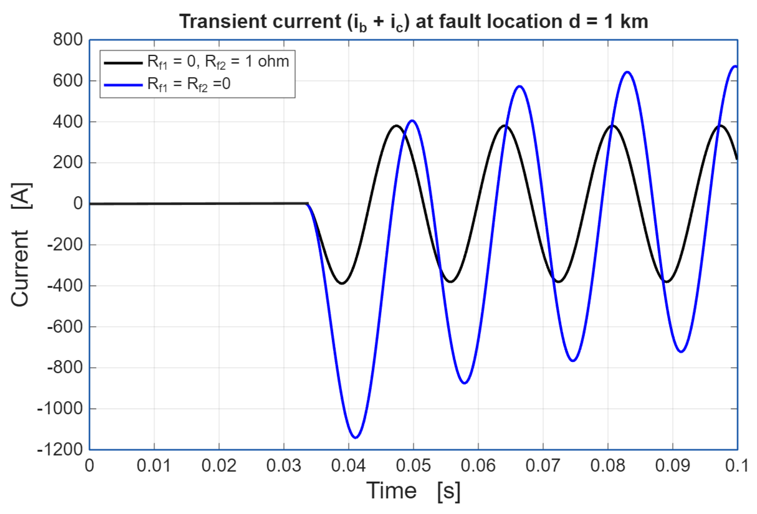
Double-phase grounded faults, described in Section 4.2, have been implemented in Matlab/Simscape in order to validate the analytical results. In particular, the currents i α and i β and the corresponding fault current i b + i c were evaluated at a fault location d = 10   km for two different values of fault resistance, i.e., R f 2 = 0 and R f 2 = 1   , with R f 1 = 0 (see Figure 26). A lower value of R f 2 results in a larger excursion of the fault current and a larger time constant. This behavior is more evident in Figure 27 where the fault location is d = 1   km. Indeed, in this case, the line parameters have a lower impact, and therefore, the fault current has a larger excursion in the case of a fault with zero resistance.
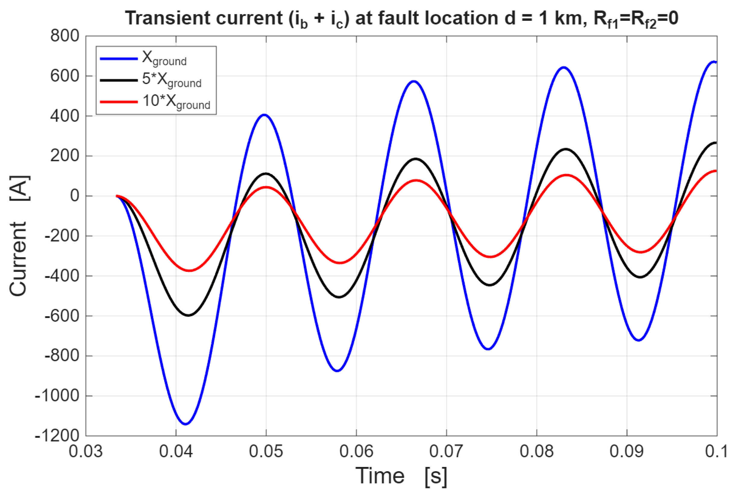
Figure 28 shows the behavior of the transient fault current i b + i c for different values of the generator ground reactance X g r . Clearly, as expected, by increasing the ground reactance, the fault current decreases.
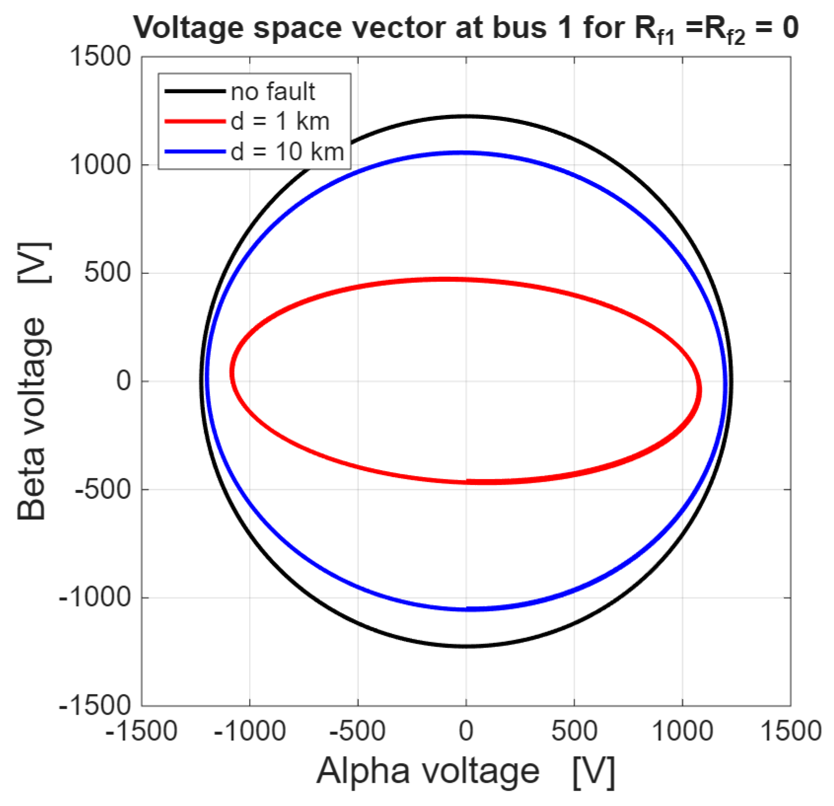
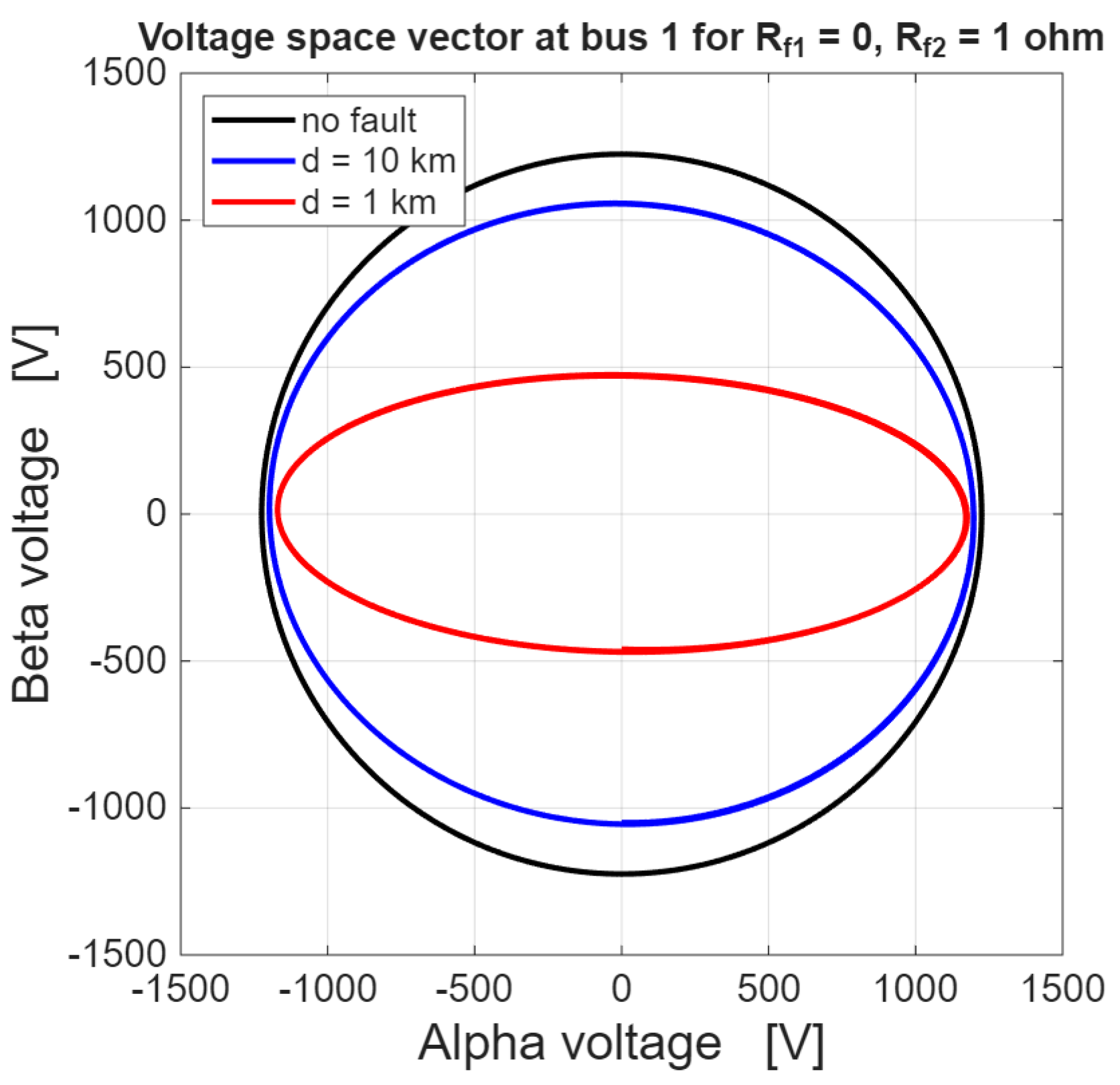
Figure 29 shows the behavior of the voltage space vector at bus 1 in the case of a fault with R f 2 = 0 . The black curve shows the circular ideal trajectory in the case of no fault. The blue curve shows the trajectory in the case of a fault location d = 10   km, whereas the red curve shows the trajectory in the case of a fault location d = 1   km. Clearly, at a smaller distance, the detection of the double-phase fault becomes more evident since the elliptical trajectory with inclination angle 0° can be readily detected. Figure 30 shows the voltage space vector in the case of a fault with R f 2 = 1   . Notice that, according to the analytical results, the fault resistance R f 2 affects only the α component, not the β component. In fact, the red curves in Figure 29 and Figure 30 have a different horizontal excursion, but they keep the same vertical excursion. The detection capability of the space vector trajectory remains effective since the phase-to-phase fault resistance R f 1 is kept to zero.

6.3. Double-Phase Ungrounded Faults

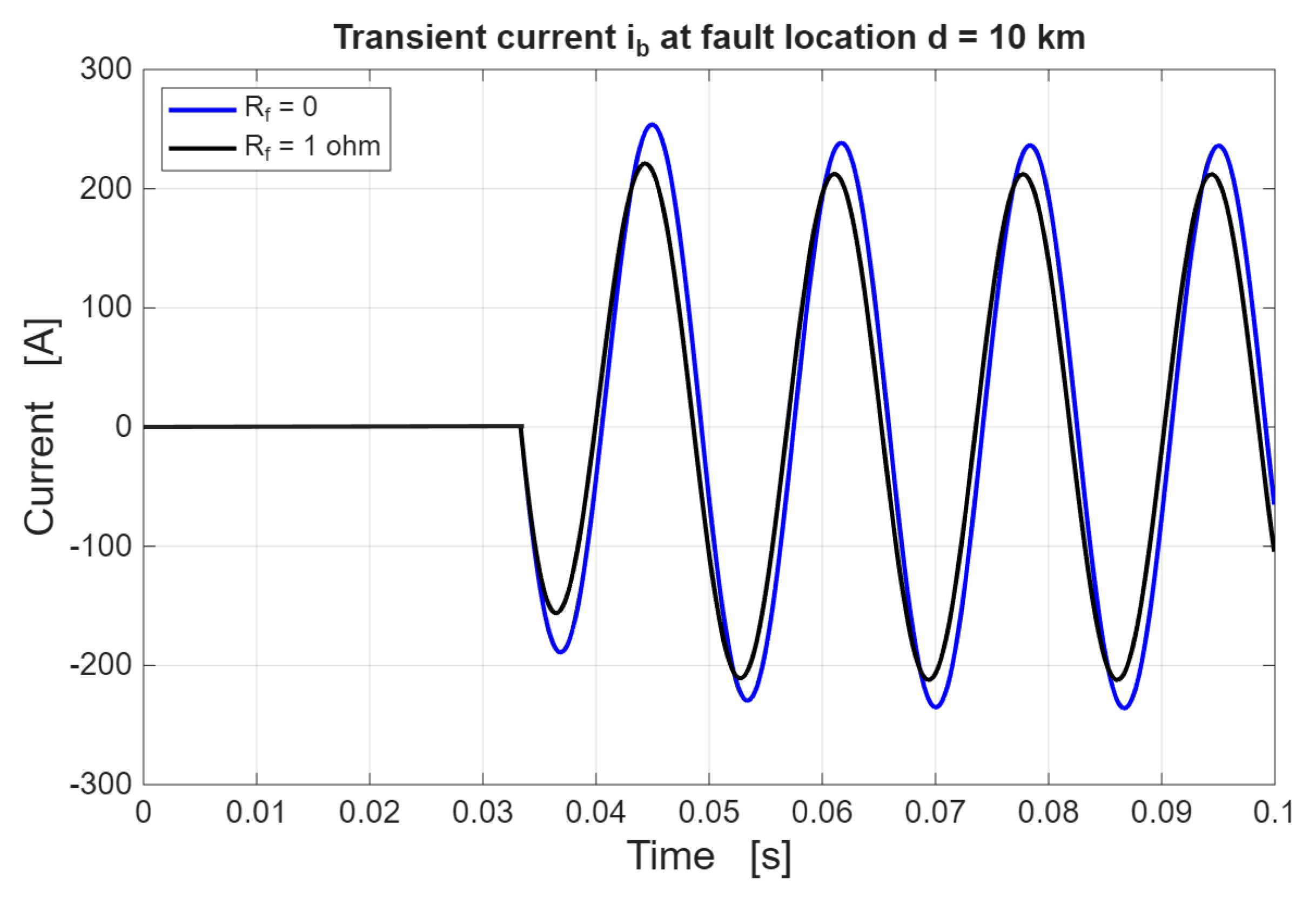
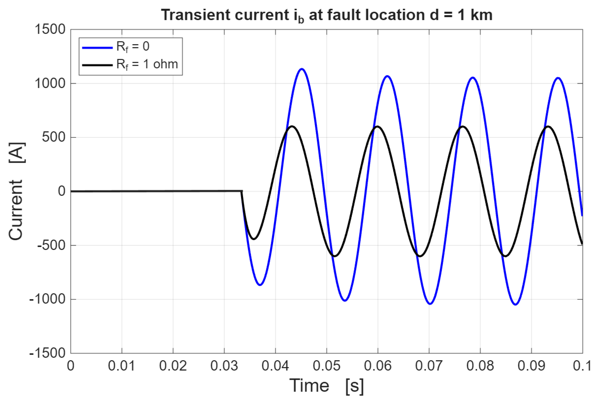
Double-phase ungrounded faults, described in Section 4.3, have been implemented in Matlab/Simscape in order to validate the analytical results. In particular, the currents i β and the corresponding fault current i b = i β / 2 were evaluated at a fault location d = 10   km for two different values of fault resistance, i.e., R f = 0 and R f = 1   (see Figure 31). A lower value of R f results in a larger excursion of the fault current and a larger time constant. This behavior is more evident in Figure 32, where the fault location is d = 1   km. Indeed, in this case, the line parameters have a lower impact, and therefore, the fault current has a larger excursion in the case of a fault with zero resistance.
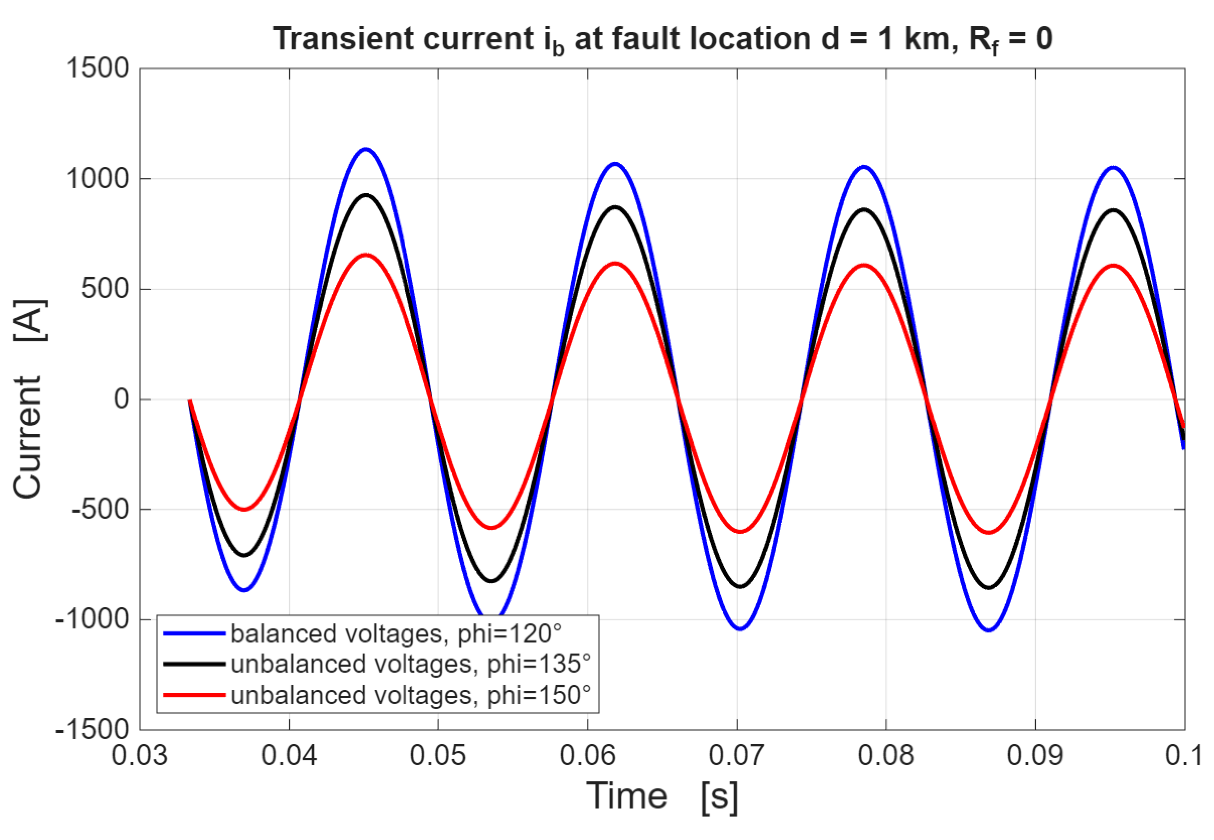
Figure 33 shows the effect of voltage unbalance on the transient fault current i b . The blue curve corresponds to the balanced case, already represented in Figure 32, where the generator voltages E b and E c have phase displacement ± 120 ° with respect to E a . The black curve corresponds to the unbalanced case, where E b and E c have phase displacement ± 135 ° with respect to E a . The red curve corresponds to the unbalanced case where E b and E c have phase displacement ± 150 ° with respect to E a . Notice that by increasing the phase displacement with respect to E a , the voltage source e β in Figure 18 decreases its magnitude. Thus, a corresponding decrease in the transient fault current in Figure 33 can be observed.
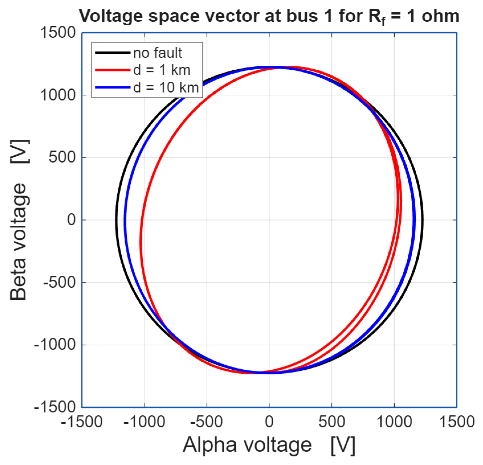
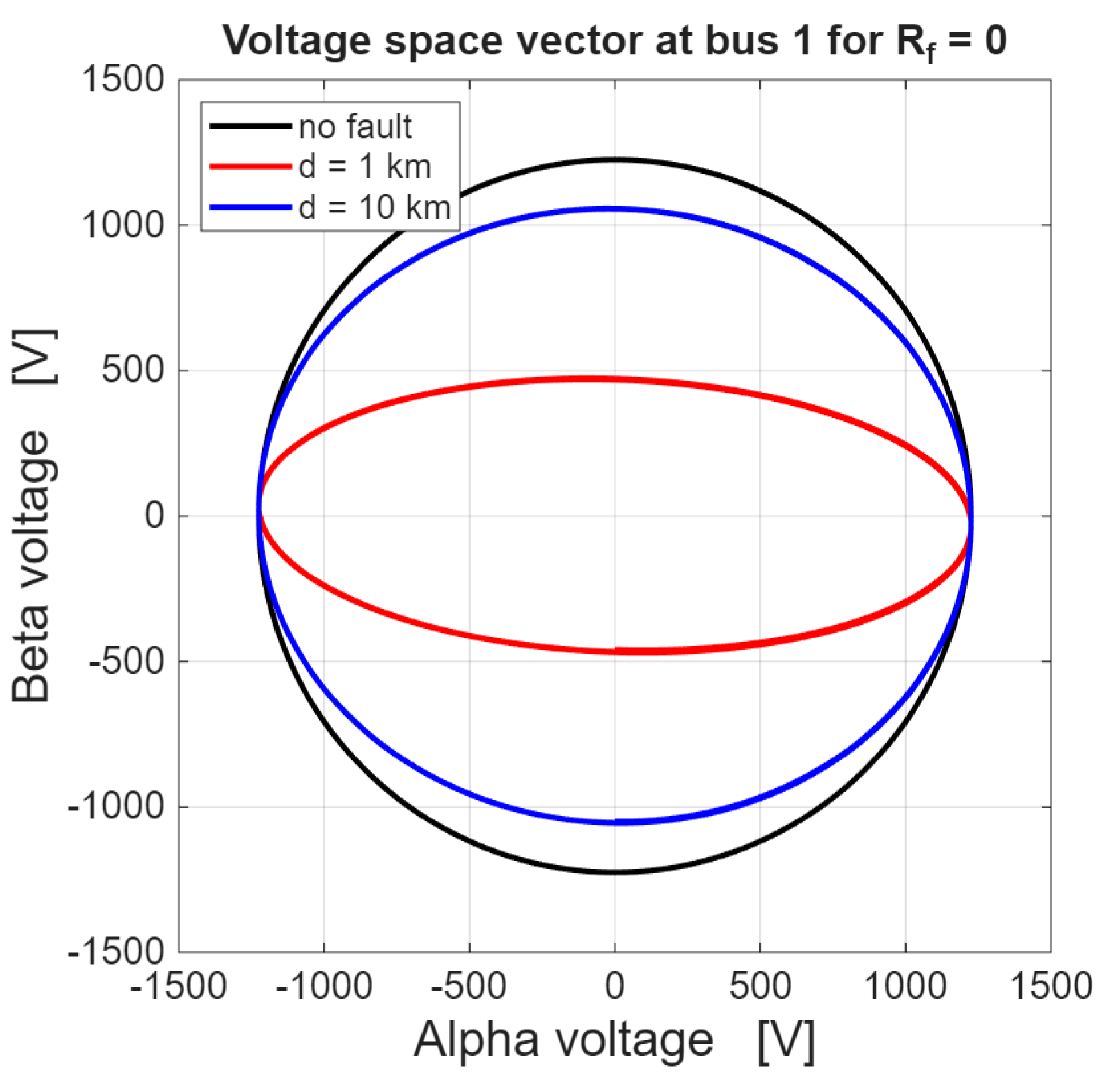
Figure 34 shows the behavior of the voltage space vector at bus 1 in the case of a fault with R f = 0 . The black curve shows the circular ideal trajectory in the case of no fault. The blue curve shows the trajectory in the case of a fault location d = 10   km, whereas the red curve shows the trajectory in the case of a fault location d = 1   km. Clearly, at a smaller distance, the detection of the double-phase fault becomes more evident, since the elliptical trajectory with inclination angle 0° can be readily detected. Figure 35 shows the voltage space vector in the case of a fault with R f = 1   . Notice that, according to the analytical results, the fault resistance R f affects only the β component, not the α component. In fact, the red curves in Figure 34 and Figure 35 have a different vertical excursion, but they keep the same horizontal excursion. Notice that the fault resistance results in a slight deviation of the ellipse inclination and a smaller difference between d = 1   km and d = 10   km. Thus, as was expected, faults with a larger resistance result in lower detection capability of the space vector trajectory. The transient behavior is also evident in the blue and red curves.

7. Conclusions

The systematic analytical investigation of the Clarke transient analysis of asymmetrical faults in three-phase systems was presented and compared with the ISCT approach. The proposed Clarke approach proved to be advantageous for two main reasons. First, the derived equivalent circuits are defined in terms of real-valued voltages and currents. Second, the dynamic order of the Clarke equivalent circuits is lower than the corresponding ISCT circuits because the αβ0 circuits are not all coupled. Thus, the main results of the paper have a theoretical value when compared with the ISCT, whereas the application domain is the same as that of the ISCT.
Future work will be devoted to extending the proposed methodology to simultaneous faults and phase interruptions.

Funding

This research received no external funding.

Data Availability Statement

The original contributions presented in this study are included in the article. Further inquiries can be directed to the corresponding author(s).

Conflicts of Interest

The author declares no conflicts of interest.

References

  1. Bollen, N.; Styvaktakis, E.; Yu-Hua Gu, I. Categorization and analysis of power system transients. IEEE Trans. Power Deliv. 2005, 20, 2298–2306. [Google Scholar] [CrossRef]
  2. Tleis, N. Power Systems Modeling and Fault Analysis, 2nd ed.; Academic Press: Cambridge, MA, USA, 2019. [Google Scholar]
  3. Chicco, G.; Mazza, A. 100 years of symmetrical components. Energies 2019, 12, 450. [Google Scholar] [CrossRef]
  4. Duesterhoeft, W.C.; Schulz, M.W.; Clarke, E. Determination of instantaneous currents and voltages by means of alpha, beta, and zero components. AIEE Trans. 1951, 70, 1248–1255. [Google Scholar] [CrossRef]
  5. Hsiao, T. Fault analysis by modified alpha, beta, and zero components—Parts I–II. AIEE Trans. Part III 1962, 81, 136–146. [Google Scholar] [CrossRef]
  6. Martinez-Velasco, J.A. Transient Analysis of Power Systems; John Wiley & Sons: Hoboken, NJ, USA, 2015. [Google Scholar]
  7. Zanetta, L.C., Jr. Understanding Electromagnetic Transients in Power Systems; IEEE Press: Piscataway, NJ, USA, 2025. [Google Scholar]
  8. Stankovic, A.M.; Aydin, T. Analysis of asymmetrical faults in power systems using dynamic phasors. IEEE Trans. Power Syst. 2000, 15, 1062–1068. [Google Scholar] [CrossRef]
  9. Ghimire, P.; Poudel, S.; Shirazi, M.; Hummels, D.M.; Tonkoski, R. Application of phasor modeling in power systems: A review. IEEE Access 2026, 14, 28573–28594. [Google Scholar] [CrossRef]
  10. Lyon, W. Transient Analysis of Alternating-Current Machinery; John Wiley & Sons: New York, NY, USA, 1954. [Google Scholar]
  11. Paap, G.C. Symmetrical components in the time domain and their application to power network calculations. IEEE Trans. Power Syst. 2000, 15, 522–528. [Google Scholar] [CrossRef]
  12. Miao, Z.; Fan, L. A Laplace-domain circuit model for fault and stability analysis considering unbalanced topology. IEEE Trans. Power Syst. 2023, 38, 1787–1790. [Google Scholar] [CrossRef]
  13. Owen, M. Transient analysis using component transforms. In Proceedings of the PEAM 2011: IEEE Power Engineering and Automation Conference, Wuhan, China, 8–9 September 2011. [Google Scholar]
  14. Dell’Olmo, J.; Gatta, F.M.; Geri, A.; Graziani, M.; Lauria, S.; Maccioni, M. Clarke transform based fast assessment of switching overvoltages in an MV distribution network. Electr. Power Syst. Res. 2022, 212, 108255. [Google Scholar] [CrossRef]
  15. Aller, J.M.; Bueno, A.; Paga, T. Power system analysis using space-vector transformation. IEEE Trans. Power Syst. 2002, 17, 957–965. [Google Scholar] [CrossRef]
  16. Bellan, D.; Superti-Furga, G. Space-vector state-equation analysis of three-phase transients. J. Electr. Syst. 2018, 14, 188–198. [Google Scholar]
  17. Bellan, D. Clarke transformation solution of asymmetrical transients in three-phase circuits. Energies 2020, 13, 5231. [Google Scholar] [CrossRef]
  18. Bellan, D. Analytical investigation of the properties of transients in unbalanced three-phase four-wire networks. Energies 2022, 15, 9122. [Google Scholar] [CrossRef]
  19. Ignatova, V.; Granjon, P.; Bacha, S. Space vector method for voltage dips and swells analysis. IEEE Trans. Power Deliv. 2009, 24, 2054–2061. [Google Scholar] [CrossRef]
  20. Alam, M.R.; Muttaqi, K.M.; Bouzerdoum, A. Characterizing voltage sags and swells using three-phase voltage ellipse parameters. IEEE Trans. Ind. Appl. 2015, 51, 2780–2790. [Google Scholar] [CrossRef]
  21. Camarillo-Peñaranda, J.R.; Ramos, G. Fault classification and voltage sag parameter computation using voltage ellipses. IEEE Trans. Ind. Appl. 2019, 55, 92–97. [Google Scholar] [CrossRef]
  22. Camarillo-Peñaranda, J.R.; Ramos, G. Characterization of voltage sags due to faults in radial systems using three-phase voltage ellipse parameters. IEEE Trans. Ind. Appl. 2018, 54, 2032–2040. [Google Scholar] [CrossRef]
  23. García-Sánchez, T.; Gómez-Lázaro, E.; Muljadi, E.; Kessler, M.; Molina-García, A. Approach to fitting parameters and clustering for characterizing measured voltage dips based on two-dimensional polarisation ellipses. Renew. Power Gener. IET 2017, 11, 1335–1343. [Google Scholar] [CrossRef]
  24. Bagheri, A.; Bollen, M.H.J. Space phasor model-based monitoring of voltages in three-phase systems. In Proceedings of the 18th International Conference on Harmonics and Quality of Power (ICHQP), Ljubljana, Slovenia, 13–16 May 2018. [Google Scholar]
  25. Li, S.; Xie, L.; Liu, Y. Fast Identification Method for Voltage Sag Type and Characteristic. In Proceedings of the IECON 2019—45th Annual Conference of the IEEE Industrial Electronics Society, Lisbon, Portugal, 14–17 October 2019. [Google Scholar]
  26. Bagheri, A.; Bollen, M.H.J.; Gu, I.Y.H. Improved characterization of multi-stage voltage dips based on the space phasor model. Electr. Power Syst. Res. 2018, 154, 319. [Google Scholar] [CrossRef]
  27. Alam, M.R.; Muttaqi, K.M.; Bouzerdoum, A. A new approach for classification and characterization of voltage dips and swells using 3-D polarization ellipse parameters. IEEE Trans. Power Del. 2015, 30, 1344–1353. [Google Scholar] [CrossRef]
  28. Alam, M.R.; Muttaqi, K.M.; Saha, T.K. Classification and Localization of Fault-Initiated Voltage Sags Using 3-D Polarization Ellipse Parameters. IEEE Trans. Power Deliv. 2020, 35, 1812–1822. [Google Scholar] [CrossRef]
  29. Bellan, D. Probability Density Function of Three-Phase Ellipse Parameters for the Characterization of Noisy Voltage Sags. IEEE Access 2020, 8, 185503–185513. [Google Scholar] [CrossRef]
  30. Bellan, D. Clarke Circuit Analysis for Space-Vector Ellipse Characterization of Phase-to-Ground Faults in Three-Phase Radial Systems. WSEAS Trans. Circuits Syst. 2023, 22, 243–250. [Google Scholar] [CrossRef]
Figure 1. The voltage space vector shows an elliptical behavior on the complex plane, where the inclination angle of the ellipse depends on the kind of fault. Single-phase faults (Sa,b,c) correspond to 0°, 60°, and 120°. Double-phase faults (Dab,bc,ac) correspond to 30°, 90°, and 50° [30].
Energies 19 02580 g001
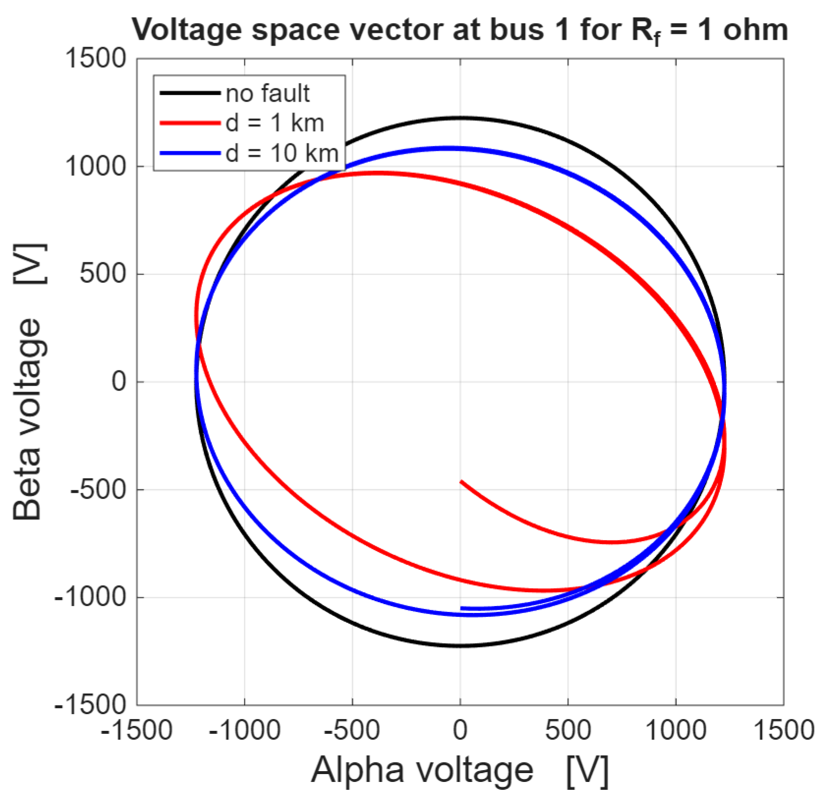
Figure 2. A star connection with a non-accessible center [30].
Energies 19 02580 g002
Figure 3. A star connection with an accessible center [30].
Energies 19 02580 g003
Figure 4. A zero-component equivalent circuit of a star connection with an accessible center [30].
Energies 19 02580 g004
Figure 5. Clarke-transformed variables at an asymmetrical fault location.
Energies 19 02580 g005
Figure 6. A single-phase fault implemented as the closure of one switch only. Fault of phase a is obtained by closing switch a.
Energies 19 02580 g006
Figure 7. Clarke circuit representation of a single-phase fault.
Energies 19 02580 g007
Figure 8. Circuit representation of double-phase grounded faults. By closing only the switches b and c, the corresponding two phases are involved in the fault.
Energies 19 02580 g008
Figure 9. Equivalent circuits in the Clarke domain for the double-phase grounded fault.
Energies 19 02580 g009
Figure 10. Circuit representation of double-phase ungrounded faults. By closing only the switches b and c, the corresponding two phases are involved in the fault.
Energies 19 02580 g010
Figure 11. Equivalent circuits in the Clarke domain for the double-phase ungrounded fault.
Energies 19 02580 g011
Figure 12. A three-phase system used to compare the Clarke and the ISCT approaches.
Energies 19 02580 g012
Figure 13. ISCT equivalent circuit for a single-phase fault.
Energies 19 02580 g013
Figure 14. Clarke equivalent circuits for a single-phase fault.
Energies 19 02580 g014
Figure 15. ISCT equivalent circuit for a double-phase grounded fault.
Energies 19 02580 g015
Figure 16. Clarke equivalent circuits for a double-phase grounded fault.
Energies 19 02580 g016
Figure 17. ISCT equivalent circuit for a double-phase ungrounded fault.
Energies 19 02580 g017
Figure 18. Clarke equivalent circuits for a double-phase ungrounded fault.
Energies 19 02580 g018
Figure 19. The radial system used to validate the analytical results. The fault location is at a distance d from bus 1.
Energies 19 02580 g019
Figure 20. Transient behavior of the phase current i a for a single-phase fault after two cycles at 60 Hz. The location of the fault is d = 10 km from bus 1, and two different values for the fault resistance are considered.
Energies 19 02580 g020
Figure 21. Transient behavior of the phase current i a for a single-phase fault after two cycles at 60 Hz. The location of the fault is d = 1 km from bus 1, and two different values for the fault resistance are considered.
Energies 19 02580 g021
Figure 22. Transient behavior of the phase current i a for a single-phase fault after two cycles at 60 Hz. The location of the fault is d = 1 km from bus 1, and three different values for the generator ground reactance are considered.
Energies 19 02580 g022
Figure 23. Transient behavior of the phase voltages v a b c for a single-phase fault with R f = 0 after two cycles at 60 Hz. The location of the fault is d = 10 km from bus 1.
Energies 19 02580 g023
Figure 24. Trajectory of the voltage space vector at bus 1 in the case of fault resistance R f = 0 . The black curve corresponds to the ideal circular trajectory in the case of no fault. The blue trajectory was obtained for a fault location d = 10   km, whereas the red trajectory corresponds to a fault location d = 1 km.
Energies 19 02580 g024
Figure 25. Trajectory of the voltage space vector at bus 1 in the case of fault resistance R f = 1   . The black curve corresponds to the ideal circular trajectory in the case of no fault. The blue trajectory was obtained for a fault location d = 10   km, whereas the red trajectory corresponds to a fault location d = 1 km.
Energies 19 02580 g025
Figure 26. Transient behavior of the fault current i b + i c for a grounded double-phase fault after two cycles at 60 Hz. The location of the fault is d = 10 km from bus 1, and two different values for the fault resistance R f 2 are considered.
Energies 19 02580 g026
Figure 27. Transient behavior of the fault current i b + i c for a grounded double-phase fault after two cycles at 60 Hz. The location of the fault is d = 1 km from bus 1, and two different values for the fault resistance R f 2 are considered.
Energies 19 02580 g027
Figure 28. Transient behavior of the fault current i b + i c for a double-phase fault after two cycles at 60 Hz. The location of the fault is d = 1 km from bus 1, and three different values for the generator ground reactance are considered.
Energies 19 02580 g028
Figure 29. Trajectory of the voltage space vector at bus 1 in the case of fault resistances R f 1 = R f 2 = 0 . The black curve corresponds to the ideal circular trajectory in the case of no fault. The blue trajectory was obtained for a fault location d = 10   km, whereas the red trajectory corresponds to a fault location d = 1 km.
Energies 19 02580 g029
Figure 30. Trajectory of the voltage space vector at bus 1 in the case of fault resistances R f 1 = 0 ,     R f 2 = 1 Ω. The black curve corresponds to the ideal circular trajectory in the case of no fault. The blue trajectory was obtained for a fault location d = 10   km, whereas the red trajectory corresponds to a fault location d = 1 km.
Energies 19 02580 g030
Figure 31. Transient behavior of the phase current i b for a double-phase ungrounded fault after two cycles at 60 Hz. The location of the fault is d = 10 km from bus 1, and two different values for the fault resistance are considered.
Energies 19 02580 g031
Figure 32. Transient behavior of the phase current i b for a double-phase ungrounded fault after two cycles at 60 Hz. The location of the fault is d = 1 km from bus 1, and two different values for the fault resistance are considered.
Energies 19 02580 g032
Figure 33. Transient behavior of the phase current i b for a double-phase fault after two cycles at 60 Hz. The location of the fault is d = 1 km from bus 1, and three different values for the generator voltage unbalance are considered.
Energies 19 02580 g033
Figure 34. Trajectory of the voltage space vector at bus 1 in the case of fault resistance R f = 0 . The black curve corresponds to the ideal circular trajectory in the case of no fault. The blue trajectory was obtained for a fault location d = 10   km, whereas the red trajectory corresponds to a fault location d = 1 km.
Energies 19 02580 g034
Figure 35. Trajectory of the voltage space vector at bus 1 in the case of fault resistance R f = 1 Ω. The black curve corresponds to the ideal circular trajectory in the case of no fault. The blue trajectory was obtained for a fault location d = 10   km, whereas the red trajectory corresponds to a fault location d = 1 km.
Energies 19 02580 g035
Table 1. Data of the components in the radial system depicted in Figure 14.
ComponentsConnectionParameters
GeneratorGrounded Y Pos . / neg . :   R = 0.1   Ω ,   X = 0.4   Ω
Zero :   X 0 = 0.2   Ω ,   Ground :   X g r = 0.2   Ω
TransformerGrounded Y-Y, 1/1 kV Pos . / neg . :   X = 0.1   Ω
Zero :   X 0 = 0.05   Ω
Line Pos . / neg . :   R = 0.1   Ω / k m ,   X = 0.3   Ω / k m
Zero :   X 0 = 0.9   Ω / k m
Load S = 10   M V A , p f = 0.9  
Disclaimer/Publisher’s Note: The statements, opinions and data contained in all publications are solely those of the individual author(s) and contributor(s) and not of MDPI and/or the editor(s). MDPI and/or the editor(s) disclaim responsibility for any injury to people or property resulting from any ideas, methods, instructions or products referred to in the content.