Reliability Assessment of AC/DC Hybrid Distribution Networks with Large-Scale Renewable Energy Integration

Abstract

With the advancement of carbon peaking and carbon neutrality goals, the increasing penetration of renewable energy sources such as wind and photovoltaic power poses severe challenges to the power supply reliability of AC/DC hybrid distribution networks due to their fluctuating, intermittent, and stochastic outputs. This paper proposes a reliability assessment method for AC/DC hybrid distribution networks under large-scale renewable energy integration based on clustering of typical operating scenarios. The net load duration curve is adopted as the feature variable to characterize typical operating scenarios. An improved t-distributed Stochastic Neighbor Embedding (t-SNE) nonlinear dimensionality reduction method with Kullback–Leibler (KL) divergence elbow correction is proposed for effective reduction of high-dimensional time-series data. An adaptive Density-Based Spatial Clustering of Applications with Noise (DBSCAN) parameter optimization method based on the k-nearest-neighbor curve and a secondary K-means clustering method based on entropy-weighted multi-objective optimization are further developed, forming a hybrid t-SNE-DBSCAN–K-means clustering algorithm. The power supply reliability is then assessed based on the clustered typical operating scenarios. A typical AC/DC hybrid distribution network is used as the test system. Results show that the DB index of the proposed clustering method improves by at least 22% compared with conventional methods, the maximum relative error between the typical-day-based and full time-series simulation results is less than 6%, and the computational efficiency improves by about 8.8 times, achieving a good balance between accuracy and efficiency.

1. Introduction

With the further implementation of the carbon peaking and carbon neutrality policy, the installed capacity and power generation share of clean energy sources, represented by wind power [1] and photovoltaic power [2], have increased year by year in power systems. AC/DC hybrid distribution networks have become an important development direction for modern distribution systems, because of their advantages in renewable energy accommodation, power supply flexibility, and power quality. However, wind generation and solar generation are greatly affected by weather conditions. Their outputs are usually volatile, intermittent, and stochastic. This brings great challenges to the operation control and power supply security of AC/DC hybrid distribution networks [3,4]. In extreme cases, it may lead to wind and solar curtailment and equipment overload, and even affect system stability. In addition, the coupling characteristics between the AC and DC subsystems further increase the complexity of reliability analysis in AC/DC hybrid distribution networks. Therefore, it has become an important research direction in new-type power systems to assess the power supply reliability of AC/DC hybrid distribution networks with large-scale renewable energy integration [5,6,7]. In power system planning, design, and reliability assessment, a common approach is to select representative or typical days as typical operating scenarios of the power system [8,9]. These limited scenarios are used to characterize power generation, transmission, and consumption behaviors over a long time scale. By analyzing the operating characteristics of these typical scenarios, the workload of system analysis can be significantly reduced. This avoids calculating all system states one by one. This approach is especially important for new-type power systems with high shares of stochastic renewable energy.

Large-scale integration of renewable energy sources, such as wind and photovoltaic power, also brings significant uncertainty to grid power. This poses severe challenges to the secure operation of AC/DC hybrid distribution networks. To address power system planning and dispatch problems under uncertainty, the mainstream research methods mainly include time-series analysis [10], uncertainty-based Monte Carlo simulation [11], and scenario generation methods [12,13,14]. Among them, scenario generation has been widely used in dispatch and planning studies [15,16]. The commonly used scenario generation methods can be classified into three categories: expert experience-based methods, probabilistic model-based methods, and typical-scenario-based methods. Among these methods, the experience-based method relies on experts to select a representative time period as the typical operating scenario. Because it is strongly affected by subjective factors, this method has gradually become unsuitable for scenario generation in new-type power systems dominated by stochastic renewable energy. In contrast, probabilistic model-based sampling methods use historical statistical data of generation and load. They fit probability distributions and then generate typical scenarios by combining random sampling techniques, such as Monte Carlo simulation or Latin hypercube sampling. Although this method can better capture the randomness of generation and load, it is still constrained by the law of large numbers. Stable convergence to a certain scenario can only be achieved when the sample size is sufficiently large. In addition, the generated scenario data are based on the expected distribution of historical data. They may not fully reflect actual operating conditions. Therefore, the applicability of this method is also limited.

Clustering-based scenario reduction is a typical scenario generation method supported by data-driven techniques [17,18]. By using dimensionality reduction and clustering algorithms, this method reduces a large number of operating scenarios into a limited set of typical scenarios according to specific features. While preserving the temporal characteristics of generation and load, it can effectively improve the accuracy of scenario reduction in system analysis and significantly reduce computation time. At present, it has become one of the mainstream approaches for power system scenario generation. Reference [19] proposed a typical scenario set generation method considering wind power and load based on an improved K-means clustering algorithm. This method can aggregate and reduce data within the calculation period, and it was applied to the assessment of wind power accommodation capability. Reference [20] developed an annual sequential production simulation model considering large-scale wind and solar generation from the perspective of renewable energy accommodation. The model comprehensively considers wind and solar output characteristics, load characteristics, unit peak-shaving capability, and grid transmission capacity. Reference [21] carried out a comprehensive comparative analysis of different clustering methods for generating long-term wind farm output variation curves. Reference [22] proposed an improved Adaptive-DBSCAN clustering algorithm for fault detection in photovoltaic power stations. By analyzing the key factors affecting unit power generation, the method accurately identifies variables related to generation fluctuations and uses them as inputs to the fault detection model. This improved algorithm enhances detection capability under abnormal conditions and improves model accuracy and reliability. It finally enables efficient fault identification and diagnosis for photovoltaic power stations and provides strong support for photovoltaic system operation and maintenance. Reference [23] proposed a photovoltaic power forecasting method that combines the K-means++ clustering algorithm with a Long Short-Term Memory (LSTM) network. In this method, K-means++ is first used to cluster the dataset. The clustered dataset is then used to train and test the LSTM neural network. This improves forecasting accuracy. It also optimizes the structure of the dataset, enabling the model to capture photovoltaic power variation trends more accurately and thus improving overall forecasting performance. Reference [24] proposed a multidimensional clustering method. This method searches subspaces by traversing an FP-tree storage structure and applies a defined K-Gaussian model in each subspace for clustering identification. The model divides subspace data into normal and abnormal clusters, removes redundant data, and accurately identifies abnormal data. As a result, it not only improves clustering efficiency but also enhances abnormal data detection capability, providing an effective solution for multidimensional data processing. Reference [25] used the fuzzy C-means clustering method to analyze historical load data of typical grid days and obtained representative seasonal daily load curves for weekdays. These results provide important support for load forecasting, load control, and power anomaly detection. They also offer guidance for electricity price formulation and marketing strategy optimization.

At present, studies on distribution network reliability assessment with large-scale renewable energy integration mainly focus on probabilistic modeling of renewable generation output. Among these studies, scenario clustering is often used to construct probabilistic models of renewable power output. However, with the increasing penetration of renewable energy, source-side power output shows significant uncertainty and strong volatility. Traditional deterministic operating models can no longer accurately describe the actual operating characteristics of the system. Reliability indices are closely related to the net load level at a given time. A higher net load level means a larger gap between generation capacity and load demand. It also implies a greater possible amount of load curtailment and a higher risk to power supply reliability. If the full-scenario enumeration method is used to quantify reliability under all possible renewable output states, the computational complexity will grow exponentially. As a result, the required computational resources may exceed the limits of practical engineering applications. Scenario clustering is therefore often introduced into power supply reliability assessment to reduce the computational burden. However, for reliability assessment, the temporal information of system operating parameters must be preserved. When dealing with high-dimensional time-series operating data, traditional scenario clustering methods often produce unsatisfactory clustering results because of the high dimensionality.

To address the above issues, this paper proposes a power supply reliability assessment method for AC/DC hybrid distribution networks with large-scale renewable energy integration. The daily net load duration curve is used as the feature variable to represent system operating scenarios. An improved t-SNE algorithm is adopted to achieve effective dimensionality reduction of high-dimensional time-series data. Then, a two-stage clustering strategy is developed. It combines preliminary clustering based on an improved DBSCAN algorithm with secondary clustering based on an improved K-means algorithm. In this way, typical operating scenarios of AC/DC hybrid distribution networks with large-scale renewable energy integration are generated. Based on these typical scenarios, the power supply reliability indices of the distribution network are calculated in a weighted manner. This enables an efficient and quantitative assessment of power supply reliability.

2. Dimensionality Reduction of Net Load Duration Curves Based on an Improved t-SNE

In conventional power supply reliability assessment of power systems, the output of dominant fossil-fuel generating units is generally deterministic. Therefore, the system operating mode $X_{t,f}$ can be fully described by a limited number of typical operating scenarios. However, with the integration of high-penetration renewable energy, source-side power output exhibits significant uncertainty and strong volatility. Traditional deterministic operating models can no longer accurately characterize the actual operating features of the system. If a full-scenario enumeration method is used to quantify the risk under all possible renewable output states, the computational complexity will increase exponentially. The computational burden grows with the number of renewable energy nodes n as O(2ⁿ). As a result, the required computational resources may exceed the limits of practical engineering applications. For this reason, scenario clustering is often used in risk assessment studies. However, in power supply reliability assessment, the temporal information of system operating parameters must be preserved. Traditional scenario clustering methods often fail to achieve effective clustering for sequential operating scenarios because the dimensionality of the data set is too high. Therefore, based on full consideration of the volatility and uncertainty of renewable power output, this paper performs clustering analysis of typical operating scenarios under large-scale renewable energy integration through feature variable extraction, dimensionality reduction of sequential operating parameters, and multiple clustering stages. On this basis, a quantitative calculation of the power supply reliability of the AC/DC hybrid distribution network is achieved. The power supply reliability of a power system can be quantified by comprehensively considering the probability of an event and the severity of its consequences, and it can be expressed as:

$$R_{\mathrm{isk}}(X_{t,f})={\displaystyle {\displaystyle \sum _i}p(E_i)\cdot }{\displaystyle {\displaystyle \sum _j}p(X_{t,j}|X_{t,f})\cdot S_{\mathrm{ev}}(E_i,X_{t,j})}$$

(1)

where $p(E_i)$ is the probability of fault event $E_i$; $X_{t,f}$ is the operating state of the power system at time t; $X_{t,j}$ is the j-th load level at time t; $p(X_{t,j}|X_{t,f})$ is the probability that the j-th load level occurs under operating state $X_{t,f}$; and $S_{\mathrm{ev}}(E_i,X_{t,j})$ is the severity function of fault event $E_i$ when the load level is $X_{t,j}$.

Typical operating scenarios of the power grid under large-scale renewable energy integration can be generated from the historical statistical data of regional grid operating parameters. However, grid operating parameters are numerous and heterogeneous. Therefore, appropriate feature variables must be selected to accurately describe operating scenarios. In scenario clustering analysis for power supply reliability assessment, the selection of feature variables should be closely related to the risk-driving factors of system operation. As discussed above, the power supply reliability of an AC/DC hybrid distribution network at the substation level is mainly affected by the mismatch between generation power and load power caused by faults. The risk index is therefore closely related to the net load level of the system at a given time.

The net load level refers to the difference between the load demand and the renewable power output of the system at a given time. A higher net load level indicates a larger gap between generation capability and load demand. It also implies a greater possible amount of load loss under the corresponding system state, and thus a higher level of operational risk. Therefore, the net load duration curve is adopted as the clustering feature because it compactly represents the supply–demand imbalance caused by the combined variation in renewable generation and load demand. In reliability assessment, the risk level is more directly associated with the residual demand after renewable generation is considered than with wind power, photovoltaic power, or load demand separately. Therefore, the net load duration curve can effectively characterize the distribution of operating stress related to load curtailment probability, load curtailment frequency, and expected energy not supplied.

Compared with directly clustering multidimensional time-series data of wind power, photovoltaic power, and load, this feature reduces the dimensionality of scenario representation and improves clustering efficiency, while emphasizing the overall balance state of the system. However, since the duration curve rearranges net load values by magnitude, it may weaken chronological information such as ramping behavior and short-term temporal correlations. Thus, the proposed method is more suitable for long-term, planning-oriented reliability assessment, whereas chronological multidimensional time-series modeling is still required for short-term dynamic operation or real-time control analysis.

The net load level of the system can be expressed as:

$$P_{\mathrm{NL}}(X_{t,f})={\displaystyle {\displaystyle \sum _j^{N_{\mathrm{D}}}}{P}_{\mathrm{D},j}(X_{t,f})}-{\displaystyle {\displaystyle \sum _i^{N_{\mathrm{G}}}}{P}_{\mathrm{G},i}}(X_{t,f})$$

(2)

where $P_{\mathrm{D},j}(X_{t,f})$ is the power demand of the j-th load node under operating state $X_{t,f}$; $P_{\mathrm{G},i}(X_{t,f})$ is the output power of the i-th renewable energy source under operating state $X_{t,f}$; and $N_{\mathrm{D}}$ and $N_{\mathrm{G}}$ are the numbers of load nodes and renewable energy sources.

If the historical statistical data contain daily operating parameters for a total of M system days, a daily net load matrix can be constructed by taking the system net load levels at all time periods of each day as rows and the net load levels of different days as columns:

$$D=\left[\begin{array}{cccc}{P}_{\mathrm{NL}}(X_{1,1})& P_{\mathrm{NL}}(X_{2,1})& \dots & P_{\mathrm{NL}}(X_{t,1})\\ P_{\mathrm{NL}}(X_{1,2})& P_{\mathrm{NL}}(X_{2,2})& \dots & P_{\mathrm{NL}}(X_{t,2})\\ \dots & \dots & \dots & \dots \\ P_{\mathrm{NL}}(X_{1,M})& P_{\mathrm{NL}}(X_{2,M})& \dots & P_{\mathrm{NL}}(X_{t,M})\end{array}\right]$$

(3)

where $P_{\mathrm{NL}}(X_{t,M})$ is the system net load level at time t on day M.

To avoid poor clustering performance caused by an excessively large value range due to numerical scale imbalance, the daily net load matrix in the above equation is further normalized. The normalized net load level can be expressed as:

$$P_{\mathrm{NL}}^{\prime }(X_{i,M})={\displaystyle \frac{P_{\mathrm{NL}}(X_{i,M})-\min (P_{\mathrm{NL}}(X_{i,M}))}{\max (P_{\mathrm{NL}}(X_{i,M}))-\min (P_{\mathrm{NL}}(X_{i,M}))}},i=1,2,\dots t$$

(4)

By normalizing all elements in (3), the normalized daily net load matrix can be obtained and denoted as $D^{\prime }$. Then, $D^{\prime }$ can be used as the feature variable of typical operating scenarios, and typical operating scenarios can be generated through clustering techniques.

After the normalized daily net load matrix $D^{\prime }$ of the regional power grid is obtained, scenario reduction can be carried out through clustering analysis, and typical operating scenarios with preserved temporal characteristics can be identified. In this matrix, each row consists of the net load levels at (t) time points within one day. In practical grid data acquisition systems, key parameters are usually collected and stored at 15 min intervals. Therefore, the number of time points of the net load level within one day is (t = 96). In other words, the dimension of $D^{\prime }$ is 96. When clustering is performed on high-dimensional data, data points become sparse in the high-dimensional space. As a result, clustering algorithms that rely on distance metrics may lose effectiveness in such a space. This can lead to unstable clustering results and makes it difficult to reflect the true cluster structure. Therefore, in the generation of typical operating scenarios, the high-dimensional time-series data in $D^{\prime }$ are first reduced in dimension to facilitate the subsequent clustering process.

The t-SNE algorithm, i.e., t-distributed stochastic neighbor embedding, is a nonlinear dimensionality reduction method based on manifold learning. It maps high-dimensional data samples into a low-dimensional manifold structure. It then achieves effective dimensionality reduction by solving the corresponding embedding mapping. At the same time, it can preserve the local similarity between data points. Therefore, it is suitable for dimensionality reduction of high-dimensional time-series data. The main steps of this algorithm are as follows.

(1) Probability distribution in the high-dimensional space

First, the similarity between every pair of high-dimensional data sample points should be calculated. In this process, the conditional probability $p(j\mid i)$ between two sample points is used to measure their similarity, and it can be expressed as:

$$p(j\mid i) ={\displaystyle \frac{\exp (-\frac{{‖x_{i }-x_j‖}^2}{2{\sigma }_i^2})}{{\displaystyle \sum _{k\ne j}\exp (-\frac{{‖x_{j }-x_k‖}^2}{2{\sigma }_i^2})}}}$$

(5)

The above equation means that neighboring points are selected according to the conditional probability density derived from a Gaussian distribution centered at sample point $x_{i }$. A larger conditional probability indicates a higher similarity between the two points. It also means that the point is more likely to be a neighbor of the sample point. In the equation, ${\sigma }_i$ is the width of the Gaussian kernel. Its specific value can be determined by introducing the perplexity index, which can be expressed as:

$$H_{\mathrm{per}}(p(j\mid i) )=2^{H(p(j\mid i) )}=2^{-{\displaystyle \sum _{j}p(j\mid i)\cdot {\log }_2(p(j\mid i))}}$$

(6)

By specifying the value of $H_{\mathrm{per}}(p(j\mid i) )$, the parameter ${\sigma }_i$ in the Gaussian kernel can be solved by a binary search algorithm. In practical engineering applications, the perplexity is usually set between 5 and 50.

After obtaining ${\sigma }_i$, the conditional probability between any two data points in the high-dimensional space can be calculated by using (5). To avoid directional bias between data points, the joint probability $p_{ij}$ between sample points should also be computed as:

$$p_{ij}={\displaystyle \frac{p(j\mid i) +p(i\mid j) }{2n}}$$

(7)

where n is the number of samples.

(2) Probability distribution in the low-dimensional space

Within the framework of the classical stochastic neighbor embedding algorithm, cluster crowding often occurs when high-dimensional data are reduced in dimension. Specifically, during dimensionality reduction, different cluster structures may overlap topologically because of space compression. As a result, their distinguishability is significantly reduced. It should be noted that this phenomenon essentially arises from the mismatch between the probability representations of high-dimensional and low-dimensional manifolds. In other words, the local topological relationships embedded in the high-dimensional space cannot be preserved consistently in the low-dimensional space by traditional probability modeling methods. The heavy-tailed property of the t-distribution can effectively overcome the problem of excessive compression of sample distances in the low-dimensional embedding space. By introducing the degree-of-freedom parameter of the t-distribution, nonlinear scaling of distances can be achieved. In this way, medium distances in the high-dimensional space can produce an appropriate manifold unfolding after mapping. At the same time, the separation property of long-distance samples can also be preserved. Therefore, in the low-dimensional space, the similarity between two data points is defined by a t-distribution with one degree of freedom, as follows:

$$q_{ij}={\displaystyle \frac{{(1+{‖y_i-y_j‖}^2)}^{-1}}{{\displaystyle \sum _{k\ne l}{(1+{‖y_i-y_j‖}^2)}^{-1}}}}$$

(8)

where $y_i$ is the projection of the high-dimensional data point $x_{i }$ in the low-dimensional space, i.e., the low-dimensional embedding coordinate. Its specific position should be adjusted by gradient descent.

(3) Determination of low-dimensional coordinates based on the loss function

Based on the obtained $p_{ij}$ and $q_{ij}$, a KL divergence function is constructed to measure the similarity between these two probability distributions. It is then used to determine the coordinates of data points in the low-dimensional space. The objective function of the KL divergence is given by:

$$C=KL(P||Q)={\displaystyle \sum _i{\displaystyle \sum _j(p_{ij}\cdot {\log }_2\frac{p_{ij}}{q_{ij}})}}$$

(9)

A smaller value of C indicates that $p_{ij}$ and $q_{ij}$ are closer to each other. This means that the high-dimensional distribution is more similar to the low-dimensional distribution, and the dimensionality reduction is more accurate. After obtaining C, its gradient with respect to the low-dimensional data point $y_i$ is calculated as:

$${\displaystyle \frac{\partial C}{\partial y_i}}=4{\displaystyle \sum _{j\ne i}(p_{ij}-q_{ij})\cdot (y_i-y_j){(1+{‖y_i-y_j‖}^2)}^{-1}}$$

(10)

After obtaining the partial derivatives, the iterative expression for updating the spatial positions of the low-dimensional data points can be constructed as:

$$y_i^{(h+1)}=y_i^h+\eta \cdot {\displaystyle \frac{\partial C}{\partial y_i}}+\alpha \cdot (y_i^h-y_i^{(h-1)})$$

(11)

where $y_i^h$ is the coordinate position of the low-dimensional data point at the h-th iteration; $\eta$ is the learning rate; and $\alpha$ is the momentum coefficient.

Through the above steps, dimensionality reduction of high-dimensional data based on the t-SNE algorithm can be achieved. However, as shown in (6), the calculation of the Gaussian kernel width ${\sigma }_i$ requires a manually specified perplexity. Although this value is generally set within the range of 5 to 50 based on experience, different perplexity values may lead to significantly different dimensionality reduction results and thus affect the quality of the reduced data.

Therefore, based on the conventional t-SNE algorithm, this paper proposes a t-SNE method with KL-divergence elbow correction to realize automatic optimization of the perplexity $H_{\mathrm{per}}(p(j\mid i) )$. The perplexity value at the elbow point corresponds to the critical point of diminishing returns in the KL-divergence function. This point indicates that the reduced data can preserve sufficient local structure while maintaining the global variation trend of the high-dimensional data. In this way, the reduced data can avoid being overly smoothed or excessively fragmented.

3. Typical Operating Scenario Clustering Based on an Improved K-Means Algorithm

The DBSCAN algorithm does not require the number of clusters to be specified in advance. It can adaptively determine the optimal clustering structure according to the spatial density distribution of data points. In addition, its noise identification mechanism can effectively filter out outliers or noise points in the data. This helps avoid distortion of clustering results caused by data acquisition errors or accidental recording errors. This characteristic makes DBSCAN particularly suitable for handling possible abnormal values in power grid operating data and ensures the accuracy of typical scenario extraction.

The core principle of the DBSCAN algorithm is based on the concept of density reachability. First, the neighborhood radius, namely Epsilon (Eps), and the neighborhood density threshold, namely Minimum Points (MinPts), are defined to determine the neighborhood range of each data point. Then, the number of data points contained in the neighborhood is used to determine whether the point is a core point. For each core point, all points within its neighborhood are assigned to the same cluster. The other points in the neighborhood are then visited recursively. If these points also satisfy the core point condition, the cluster continues to expand until no new core points can be found. In essence, this algorithm performs clustering by identifying high-density regions in the dataset, while low-density regions are excluded from the clustering results. This density-based clustering mechanism enables the algorithm to effectively discover clusters with arbitrary shapes and automatically identify noise data.

However, two parameters in the DBSCAN algorithm must be determined, namely the neighborhood radius and the neighborhood density threshold. The former is also called the radius parameter. It represents the radius of the neighborhood around a data point. In the dataset, the region within a distance of Eps from a data point is called the neighborhood of that point. The latter is also called the minimum number of points. It represents how many data points must exist within the neighborhood of a data point for that point to be defined as a core point. In the conventional DBSCAN algorithm, the values of Eps and MinPts are usually set empirically and then adjusted repeatedly according to the clustering results. This process is highly subjective. Therefore, this paper uses the k-nearest-neighbor distance curve to automatically identify the above two parameters.

Before presenting the steps of the improved DBSCAN algorithm, the variables used in the algorithm are first defined.

Definition 1.

Eps neighborhood: The Eps neighborhood refers to the region centered at a data point with Eps as the radius, and it is expressed as:

$$N_{Esp}(y_i)=\{y_j\in D_y^{\prime }|‖y_i-y_j‖\le Eps\}$$

(12)

In the above equation, $D_y^{\prime }$ is the mapping matrix of $D^{\prime }$ in the low-dimensional space. Then, the Eps neighborhood contains all data points in matrix $D_y^{\prime }$ whose distances to object $y_i$ do not exceed Eps.

Definition 2.

Core point: If the Eps neighborhood of data point  $y_i$  contains at least MinPts data points, then  $y_i$  is called a core point, which can be expressed as:

$$\left|N_{Esp}(y_i)\right|\ge MinPts$$

(13)

Definition 3.

Noise point: A noise point is a point that is neither a core point nor contained in the Eps neighborhood of any core point.

Based on the above definitions, the basic steps of the improved DBSCAN clustering algorithm proposed in this paper for the adaptive determination of Eps and MinPts are given as follows.

First, for any two data points $y_i$ and $y_j$ in the dimension-reduced dataset $D_y^{\prime }$, the Euclidean distance between them is calculated as:

$$d_{ij}={‖y_i-y_j‖}_2,\forall i,j\in \{1,2,\dots M\}$$

(14)

The calculated distances are then combined to form the distance distribution matrix $dist=\left\{d_{ij}\right|\forall i,j\in \{1,2,\dots M\}\}$ of dataset $D_y^{\prime }$.

Next, the elements in each row of matrix $dist$ are sorted in ascending order to form a new matrix $dis{t}_{\mathrm{K}}$. This matrix is called the k-nearest-neighbor matrix. The element in the k-th column represents the distance from a data point in dataset $D_y^{\prime }$ to its k-th nearest neighbor.

On this basis, the average value of each column of matrix $dis{t}_{\mathrm{K}}$ is calculated. In this way, the k-average nearest-neighbor distances of the data points are obtained and arranged in matrix $D_y^{\prime }$. These values are taken as candidate values of Eps. The k-th average nearest-neighbor distance is denoted by Eps(k), where k = 1, 2, … m.

Furthermore, k is initialized as 1, and the corresponding Eps(k) is obtained. Substituting it into (15), the expected number of data points within the Eps neighborhood of each data point $y_i$ in dataset $D_y^{\prime }$ can be obtained as:

$$MinPts=⌊{\displaystyle \frac{1}{M}}{\displaystyle \sum _{i=1}^M\left|N_{Esp}(y_i)\right|}⌋$$

(15)

where ⌊ ⌋ denotes the floor operation.

Next, it is checked whether k ≤ m is satisfied. If not, the algorithm terminates. A curve of the number of output clusters of DBSCAN versus (k) is then plotted, and its elbow point is taken as the optimal Eps(k) and MinPts(k). If the condition is satisfied, the DBSCAN input parameters Eps(k) and MinPts(k) are initialized. Meanwhile, the DBSCAN cluster label set is initialized as Labels = {L_C}. The current cluster index is initialized as L_C = 0. The data point index is initialized as i = 1. The visit flags of all data points are initialized to 0 in $v=\{v_1,v_2,\dots v_i,\dots v_M\}$.

Then, it is checked whether condition $\left|N_{Esp}(y_i)\right|\ge MinPts$ is satisfied. If not, the point is marked as a noise point, and i = i + 1 is set to process the next data point. If condition $\left|N_{Esp}(y_i)\right|\ge MinPts$ is satisfied, the point is regarded as a core point. A new cluster C is created, and its cluster index is set to the current maximum cluster index plus 1, i.e., L_C = max(L_C) + 1. The algorithm then enters the cluster expansion stage. Next, an empty set Q is created. Data point $y_i$ and all points in its neighborhood are added into set Q. At the same time, the data index is initialized as j = 1.

For any data point $y_j$ in Q, it is checked whether the stopping condition is satisfied $v_j=1$. If it is satisfied, the current cluster expansion is completed. Otherwise, the following steps are performed. It is first determined whether the data point $y_j$ has been visited, i.e., whether v_j = 1 is satisfied. If yes, let j = j + 1, and continue to determine whether this point is a core point. Otherwise, let v_j = 1, let j = j + 1, and directly add the data point $y_j$ to set Q, and then continue to process the next data point. It is further determined whether $y_j$ is a core point. If yes, all points in its neighborhood are added to set Q. Otherwise, the data point $y_j$ is directly added to set Q, and j = j + 1 is set to continue processing the next point in the set. When $y_i\in D_y^{\prime }$, for any data point, v_i = 1 is satisfied, all clustering results are output, the number of clusters corresponding to the current Eps(k) and MinPts(k) is recorded, and k = k + 1 is set. The algorithm then returns to check whether k ≤ m holds, and the above process is repeated until all k values have been traversed. Otherwise, the current cluster continues to expand.

By applying the above algorithm to the dimension-reduced dataset $D_y^{\prime }$, the preliminary clustering results can be obtained. Each cluster contains several data points with similar features. However, validation results show that, because the renewable generation output curves exhibit strong randomness, one round of clustering alone cannot guarantee satisfactory classification results. Therefore, based on the preliminary clustering by DBSCAN, this paper further performs secondary clustering using an improved K-means algorithm, so as to obtain more accurate clustering results.

(1) Optimization of Initial Cluster Centroids Based on K-means++

After preliminary clustering is performed on the dimension-reduced dataset $D_y^{\prime }$, suppose that all data points in $y_i\in D_y^{\prime }$ are divided into H_1st clusters, and the h cluster is denoted by H_1st(h). In this section, secondary clustering based on the improved K-means algorithm is further carried out for each cluster to improve clustering accuracy.

K-means clustering is a typical unsupervised machine learning algorithm. Its core idea is to partition a dataset into K disjoint clusters through iterative optimization. Given the cluster number K, the algorithm performs clustering by minimizing the sum of squared Euclidean distances between data points and the centroids of their assigned clusters. Specifically, the algorithm alternately performs the following two steps: assigning data points according to the current centroids, and updating the centroid positions according to the current cluster members, until the convergence condition is satisfied. However, in the conventional K-means algorithm, the initial centroids are selected randomly. As a result, the algorithm is prone to falling into a local optimum and cannot guarantee a globally optimal clustering result. Therefore, this paper adopts the K-means++ algorithm to optimize the selection of the initial centroids and reduce the probability of convergence to a local optimum.

The specific procedure of the secondary clustering method based on the improved K-means++ proposed in this paper is as follows:

First, initialize the cluster index as h = 1, and set the number of clusters for secondary clustering as K. It is then checked whether h ≤ H_1st is satisfied. If yes, initialize the centroid index as k = 1, and calculate the number of data points in cluster H_1st(h), denoted by N_h. Then, randomly select one data point $y_i\in H_{1\mathrm{st}}(h),i=1,2,\dots N_h$ from this cluster as the first cluster centroid, denoted by c_k. Otherwise, the calculation ends. Next, it is checked whether k ≤ K is satisfied. If yes, calculate the minimum distance between each of the other data points in the cluster and c_k as:

$$d_{jk}=\min {‖y_j-c_k‖}^2$$

(16)

If the condition is not satisfied, it means that K initial centroids for secondary clustering have been obtained, and the algorithm then enters the iterative clustering stage.

During the determination of the initial centroids, the following equation is used to calculate the probability that each data point in the cluster is selected as the next cluster centroid:

$$p(y_j)={\displaystyle \frac{d_{jk}}{{\displaystyle \sum _{j=1}^{N_h}{d}_{jk}}}}$$

(17)

The above equation indicates that a data point with a larger minimum distance from the existing centroids has a higher probability of being selected as the next initial centroid. According to this probability distribution, the centroid of the next cluster is determined by weighted random sampling. Then, let k = k + 1, and continue to check whether k ≤ K holds.

After the initial centroids are determined, the following equation is used as the objective function of the secondary clustering to assign each data point to a cluster:

$$\arg \underset{C}{\min }J(C)={\displaystyle {\displaystyle \sum _{k=1}^K}{\displaystyle \sum _{y_i\in C_k}{‖y_i-c_k‖}_2^2}}$$

(18)

where $J(C)$ is the objective function of the K-means algorithm. The goal is to optimize the cluster centroids C so that the sum of squared Euclidean distances from all data points in each cluster to the corresponding centroid is minimized. $C_k$ denotes the set of all data points in the k-th cluster.

For the specific assignment process, the squared Euclidean distance from each data point $y_i$ to each centroid $c_k$ is first calculated as:

$${‖y_i-c_k‖}_2^2={\displaystyle \sum _{l=1}^m(y_{i,l}-c_{j,l}}{)}^2$$

(19)

where l is the l-th feature of $y_i$, and the data point has m dimensions in total.

Each data point is then assigned to the nearest cluster centroid. According to the current cluster partition, the position of each centroid is updated by using the mean of all sample points in the cluster, i.e.,

$$c_k={\displaystyle \frac{1}{\left|C_k\right|}}{\displaystyle \sum _{y_i\in C_k}{y}_i}$$

(20)

where $\left|C_k\right|$ is the number of data points in the k-th cluster.

Equations (19) and (20) are repeated until the cluster centroids at the (t + 1)-th iteration no longer change significantly compared with those at the t-th iteration, i.e.,

$$\left|c_k^{(t+1)}-c_k^{(t)}\right|\le \epsilon$$

(21)

where $\epsilon$ is the given convergence threshold.

After convergence is reached, (19) is used again to calculate the distance between each data point $y_i\in H_{1\mathrm{st}}(h)$ and each centroid c. Each data point is then assigned to the cluster represented by its nearest centroid. In this way, the secondary clusters corresponding to the preliminary cluster H_1st(h), namely C₁, C₂, …C_K, are obtained. Then, let h = h + 1, and return to check whether h ≤ H_1st(h) holds. The above process is repeated until secondary clustering has been completed for all preliminary clusters.

(2) Calculation model of the optimal cluster number K based on Silhouette Coefficient (SC) and the Davies–Bouldin Index (DB) multi-objective optimization with the entropy weight method

By following the above steps, the optimal secondary clustering result for all data points in H_1st(h), can be obtained under a given value of K. However, as mentioned above, the clustering performance is highly dependent on the preset value of K. In most cases, the optimal value of K is unknown in advance. It is often determined only after repeated manual trials based on experience, which makes the clustering result subjective. To overcome the limitation of the conventional K-means algorithm and reduce the subjectivity of manually setting the cluster number K, this paper proposes a multi-index fusion evaluation strategy based on the entropy weight method. Specifically, by combining the quantitative analysis of the SC-DB, an automatic optimization model for selecting the value of K is constructed. This method uses the entropy weight method to assign objective weights and balance the contributions of clustering compactness, represented by SC, and inter-cluster separability, represented by DB. In this way, the optimal value of K can be determined adaptively. The specific procedure is as follows:

For $1\le K\le \sqrt{M},K\in {\mathbb{N}}^{*}$, each possible value of K is taken as an input, and the steps described in the previous subsection are used to perform secondary clustering on $D_y^{\prime }$. For each $H_{1\mathrm{st}}(h)\subset D_y^{\prime }$, K secondary clusters can be obtained, denoted by $H_{2\mathrm{nd}}\left(q\right)$, where $H_{2\mathrm{nd}}(q)\subset H_{1\mathrm{st}}(h),q=1,2,\dots K$. For each $H_{2\mathrm{nd}}\left(q\right)$, the average distance between data point i within the cluster and the other data points in the same cluster is calculated as:

$$d_{ij}^{\mathrm{IC}}={\displaystyle \frac{1}{\left|H_{2\mathrm{nd}}(q)\right|-1}}\cdot {\displaystyle \sum _{y_j\in H_{2\mathrm{nd}}(q),j\ne i}{‖y_i-y_j‖}_2}$$

(22)

where $\left|H_{2\mathrm{nd}}\left(q\right)\right|$ is the number of data points in the cluster.

The average distance from data point $y_i$ to all data points in each of the other clusters $H_{2\mathrm{nd}}(b)\subset H_{1\mathrm{st}}(h), b=1,2,\dots K\&b\ne q$ is calculated. The minimum of these distances is taken as the inter-cluster Euclidean distance:

$$d_{ij}^{\mathrm{BC}}=\min {\displaystyle \frac{1}{\left|H_{2\mathrm{nd}}(b)\right|}}{\displaystyle \sum _{y_j\in H_{2\mathrm{nd}}(b)}{‖y_i-y_j‖}_2}$$

(23)

By combining (22) and (23), the SC $sc(y_i)$ of a single data point $y_i$ can be obtained, which is expressed as:

$$sc(y_i)={\displaystyle \frac{d_{ij}^{\mathrm{BC}}-d_{ij}^{\mathrm{IC}}}{\max (d_{ij}^{\mathrm{BC}},d_{ij}^{\mathrm{IC}})}}$$

(24)

As can be seen from the above equation, when the inter-cluster distance $d_{ij}^{\mathrm{BC}}$ of data point $y_i$ is much larger than its intra-cluster distance $d_{ij}^{\mathrm{IC}}$, the value of the SC approaches 1. This indicates that the point has been assigned to the correct cluster. Otherwise, it indicates that the point has been assigned to an incorrect cluster. By averaging the SC $sc(y_i)$ of all data points $y_i\in H_{1\mathrm{st}}(h)$, the SC of the overall clustering result can be obtained as:

$$SC={\displaystyle \frac{1}{\left|H_{1\mathrm{st}}(h)\right|}}\cdot {\displaystyle \sum _{y_i\in H_{1\mathrm{st}}(h)}sc(y_i)}$$

(25)

Similar to the SC, the DB index is also commonly used to evaluate clustering quality. The difference is that this index mainly measures the balance between intra-cluster compactness and inter-cluster separation. It evaluates clustering performance by comparing the relative distance between clusters with the dispersion within each cluster. For a clustering result containing K clusters, the DB index is defined as:

$$DB={\displaystyle \frac{1}{K}}{\displaystyle \sum _{q=1}^K\underset{q\ne b}{\max }(\frac{L_q^{\mathrm{IC}}+L_b^{\mathrm{IC}}}{L_{qb}^{\mathrm{BC}}})}$$

(26)

where $L_q^{\mathrm{IC}}$ is the average dispersion of the q-th cluster $H_{2\mathrm{nd}}\left(q\right)$, i.e., the intra-cluster compactness. It can be measured by calculating the average distance from all data points in the q-th cluster $H_{2\mathrm{nd}}\left(q\right)$ to the cluster centroid $c_q$:

$$L_q^{\mathrm{IC}}={\displaystyle \frac{1}{\left|H_{2\mathrm{nd}}(q)\right|}}{\displaystyle \sum _{y_i\in H_{2\mathrm{nd}}{(q)}_i}{‖y_i-c_i‖}_2}$$

(27)

where $L_{qb}^{\mathrm{BC}}$ is the Euclidean distance between the centroid $c_q$ of the q-th cluster and the centroid $c_b$ of the b-th cluster, and it is used to measure inter-cluster separation:

$$L_{qb}^{\mathrm{BC}}={‖c_q-c_b‖}_2$$

(28)

As can be seen from (26), when the intra-cluster compactness is high and the inter-cluster separation is large, the DB index is small. In contrast, when the intra-cluster compactness is low and the inter-cluster separation is small, the DB index becomes large.

Since the SC and the DB provide complementary criteria for evaluating clustering performance, a unified evaluation framework should be established through multi-index fusion. A larger SC value indicates higher intra-cluster compactness, whereas a smaller DB value reflects better inter-cluster separation. Therefore, this paper adopts the entropy weight method to address this issue.

During the secondary clustering of dataset $H_{1\mathrm{st}}(h)\subset D_y^{\prime }$, for each possible value of K, the corresponding SC and DB indices can be obtained from (25) and (26), denoted by SC_K and DB_K, respectively. The arrays formed by these SC and DB indices are denoted as:

$$\begin{array}{l}SC=\{S{C}_1,S{C}_2,\dots S{C}_{⌊\sqrt{\mathrm{M}}⌋}\}\\ DB=\{D{B}_1,D{B}_2,\dots D{B}_{⌊\sqrt{\mathrm{M}}⌋}\}\end{array}$$

(29)

To avoid the influence of the dimensional differences between the SC and DB indices on the entropy weights, these two indices are first normalized. For SC_K, max normalization is adopted:

$$S{C}_K^{\prime }={\displaystyle \frac{S{C}_K-\min (SC)}{\max (SC)-\min (SC)}}$$

(30)

Similarly, for DB_K, min normalization is adopted:

$$D{B}_K^{\prime }={\displaystyle \frac{\max (DB)-D{B}_K}{\max (DB)-\min (DB)}}$$

(31)

In this way, both indices are normalized to the range of [0, 1]. A value closer to 1 indicates better clustering performance.

In the entropy weight method, entropy reflects the degree of dispersion of an index. A larger degree of dispersion indicates a higher importance of the index. Accordingly, the information entropy values of the above two indices under K possible cluster numbers are calculated as follows:

$$\left\{\begin{array}{l}{E}_{\mathrm{SC}}=-{\displaystyle \frac{1}{\ln (⌊\sqrt{M}⌋)}}{\displaystyle \sum _{K=1}^{⌊M⌋}[p_K^{\mathrm{SC}}\cdot \ln (p_K^{\mathrm{SC}})]}\\ E_{\mathrm{DB}}=-{\displaystyle \frac{1}{\ln (⌊\sqrt{M}⌋)}}{\displaystyle \sum _{K=1}^{⌊M⌋}[p_K^{\mathrm{DB}}\cdot \ln (p_K^{\mathrm{DB}})]}\end{array}\right.$$

(32)

where $E_{\mathrm{SC}}$ and $E_{\mathrm{DB}}$ are the information entropy values of the SC index and the DB index.

$p_K^{\mathrm{SC}}$ and $p_K^{\mathrm{DB}}$ are defined as:

$$\left\{\begin{array}{l}{p}_K^{\mathrm{SC}}={\displaystyle \frac{S{C}_K}{{\displaystyle \sum _{K=1}^{⌊\sqrt{M}⌋}S{C}_K}}}\\ p_K^{\mathrm{DB}}={\displaystyle \frac{D{B}_K}{{\displaystyle \sum _{K=1}^{⌊\sqrt{M}⌋}D{B}_K}}}\end{array}\right.$$

(33)

A smaller information entropy value indicates that the index contains more effective information and should be assigned a larger weight. The weights of the SC index and the DB index are calculated by the following equations:

$$\left\{\begin{array}{l}{\omega }_{\mathrm{SC}}={\displaystyle \frac{1-E_{\mathrm{SC}}}{(1-E_{\mathrm{SC}})+(1-E_{\mathrm{DB}})}}\\ {\omega }_{\mathrm{DB}}={\displaystyle \frac{1-E_{\mathrm{DB}}}{(1-E_{\mathrm{SC}})+(1-E_{\mathrm{DB}})}}\end{array}\right.$$

(34)

For each $1\le K\le \sqrt{M},K\in {\mathbb{N}}^{*}$, the comprehensive evaluation index $S{D}_K$ obtained by the entropy weight method is calculated by the following equation:

$$S{D}_K={\omega }_{\mathrm{SC}}\cdot S{C}_K^{\prime }+{\omega }_{\mathrm{DB}}\cdot D{B}_K^{\prime }$$

(35)

A larger value of this index indicates better clustering performance. Therefore, the corresponding value of K for $\max (S{D}_K)$ can be taken as the optimal number of clusters. By substituting it into the above method, the optimal clustering result for $H_{1\mathrm{st}}(h)\subset D_y^{\prime }$ can be obtained.

4. Power Supply Reliability Assessment Method for AC/DC Hybrid Distribution Networks Based on Typical Operating Scenarios

4.1. Typical-Scenario-Based Reliability Assessment Procedure

Based on the above study, this paper proposes a typical operating scenario clustering method based on t-SNE-DBSCAN–K-means. After dimensionality reduction of high-dimensional net load time-series curves and secondary clustering, the given M net load curves can be divided into several clusters. Assume that, after the two-stage clustering process, the final number of clusters is $N_C$. Then, the set represented by the j-th cluster can be denoted by $H_{2\mathrm{nd}}(j),j=1,2,\dots N_C$. Suppose that element $y_i\in D_y^{\prime }$ in the dimension-reduced matrix belongs to the j-th cluster, and its cluster centroid is c_j. Correspondingly, in the high-dimensional net load time-series data matrix $D$, the i-th row, which represents the system net load levels at all time periods on day i, also belongs to the j-th cluster. That is, for a high-dimensional data point, $P_{\mathrm{NL} }(X_{t,i})=\{P_{\mathrm{NL}}(X_{1,i}),P_{\mathrm{NL}}(X_{2,i}),\dots P_{\mathrm{NL}}(X_{96,i})\}\in H_{2\mathrm{nd}}(j)$ holds. Suppose that the j-th cluster contains n_j such data points $P_{\mathrm{NL} }(X_{t,i})$. Then, the data points in cluster $H_{2\mathrm{nd}}(j)$ can be expressed as:

$$H_{2\mathrm{nd}}(j)=\{P_{\mathrm{NL} }(X_{t,1}),P_{\mathrm{NL} }(X_{t,2}),\dots P_{\mathrm{NL} }(X_{t,i}),\dots P_{\mathrm{NL} }(X_{t,n_j})\}$$

(36)

If the data point in $H_{2\mathrm{nd}}(j)$ corresponding to the cluster centroid c_j is denoted by $P_{\mathrm{NL}}^{c_j}(X_{t,i})$, then $P_{\mathrm{NL}}^{c_j}(X_{t,i})$ can be used to represent the net load time-series curve corresponding to this cluster. Based on this curve, the renewable generation output and load demand at all t time periods on day i can be obtained and then substituted into the power supply reliability assessment model proposed in this paper to calculate the power supply reliability indices of the AC/DC hybrid distribution network. In summary, the specific procedure for power supply reliability assessment of an AC/DC hybrid distribution network with large-scale renewable energy integration is as follows.

First, the historical statistical data containing daily operating parameters for a total of M system days are taken as the input. According to the calculation method in (2), the daily net load matrix $D$ of the system is constructed and then normalized to obtain $D^{\prime }$.

Second, the improved t-SNE model is used to reduce the dimensionality of $D^{\prime }$, and the dimension-reduced dataset is denoted by $D_y^{\prime }$.

Then, the improved DBSCAN algorithm is applied to $D_y^{\prime }$ for preliminary clustering, and H_1st clusters are obtained.

Further, all preliminary clusters are subjected to secondary clustering by using the improved K-means algorithm. In this way, N_C final clusters are obtained, and each cluster is denoted by $H_{2\mathrm{nd}}(j),j=1,2,\dots N_C$.

On this basis, the centroid $P_{\mathrm{NL}}^{c_j}(X_{t,i})$ of the j-th cluster is taken to represent the net load time-series curve corresponding to this cluster. Accordingly, the renewable generation output and load demand at all t time periods on day i represented by this centroid can be obtained.

Finally, the probability of load curtailment PLC, the expected frequency of load curtailment (EFLC), and the expected energy not supplied (EENS) are selected as the indices for power supply reliability assessment. These three indices reflect the power supply reliability risk of the AC/DC hybrid distribution network during operation from the perspectives of probability, frequency, and severity, respectively.

The AC/DC hybrid distribution network is first transformed into an equivalent capacity graph G = {V, E, C, p} by using the network topology analysis method. The source node is set as s, and the sink node is set as t. If the operating risk of only one load node is to be evaluated, the sink node t can be replaced by the node $u\in V$ where the equivalent load is located. Next, the SMC simulation method is adopted. First, the number of repeated SMC samplings is set as N_sa, the sampling period of each sample is set as T = [t₀~t_h], and the stopping criterion of sampling is set as. The sample index is initialized as n_sa = 1. Then, for the n_sa-th sample, its time-varying graph $TVG=\{V,E({\tau }_G^j),C({\tau }_G^j),p({\tau }_G^j),T\}$ is generated, and the maximum flow $f_{max}({\tau }_G^j)$ of $\mathit{G}({\tau }_G^j)$ is calculated by using the improved Dinic algorithm. Furthermore, the load demand of the load point during period T, namely, is input. To consider the most severe case, $P_{\mathrm{d}}$ can be set as the maximum possible load demand of the load point during period T. Then, the total number of times $M_{\mathrm{dn}}(n_{\mathrm{sa}})$ and the total duration $T_{\mathrm{dn}}(n_{\mathrm{sa}})$ for which the load demand is not satisfied during period T, i.e., $P_{\mathrm{d}}-f_{\max }({\tau }_G^j)>0$, can be obtained as:

$$T_{\mathrm{dn}}(n_{\mathrm{sa}})={\displaystyle \sum _{j=1}^{M_{\mathrm{dn}}(n_{\mathrm{sa}})}{{\tau }_G^j}_{\mathrm{dn}}}$$

(37)

where ${{\tau }_G^j}_{\mathrm{dn}}$ is the duration of the j-th state in which the load demand is not satisfied.

On this basis, the power supply reliability indices of the AC/DC hybrid distribution network for the n_sa-th sample during period T can be obtained by the following equations:

$$\mathrm{PLC}(n_{\mathrm{sa}})={\displaystyle \frac{T_{\mathrm{dn}}(n_{\mathrm{sa}})}{T}}$$

(38)

$$\mathrm{EFLC}(n_{\mathrm{sa}})={\displaystyle \frac{M_{\mathrm{dn}}(n_{\mathrm{sa}})}{T}}$$

(39)

$$\mathrm{EENS}(n_{\mathrm{sa}})={\displaystyle \sum _{j=1}^{M_{\mathrm{dn}}(n_{\mathrm{sa}})}[P_{\mathrm{d}}-f_{\max }({{\tau }_G^j}_{\mathrm{dn}})]\cdot {{\tau }_G^j}_{\mathrm{dn}}}$$

(40)

Finally, the coefficient of variation of the risk indices for the first n_sa samples is calculated. Taking PLC as an example, it can be expressed as:

$$\eta (\mathrm{PLC})={\displaystyle \frac{\sqrt{VA(\mathrm{PLC})}}{AR(\mathrm{PLC})}}$$

(41)

where $\eta (\mathrm{PLC})$ is the coefficient of variation of PLC; $VA(\mathrm{PLC})$ is the variance of PLC; and $AR(\mathrm{PLC})$ is the mean of PLC.

$VA(\mathrm{PLC})$ and $AR(\mathrm{PLC})$ can be obtained by the following equations, respectively:

$$VA(\mathrm{PLC})={\displaystyle \frac{1}{n_{\mathrm{sa}}(n_{\mathrm{sa}}-1)}}{\displaystyle \sum _{i=1}^{n_{\mathrm{sa}}}{\left[\mathrm{PLC}\right(i)-AR(\mathrm{PLC})]}^2}$$

(42)

$$AR(\mathrm{PLC})={\displaystyle \frac{1}{n_{\mathrm{sa}}}}{\displaystyle \sum _{i=1}^{n_{\mathrm{sa}}}\mathrm{PLC}(i)}$$

(43)

Moreover, if the following condition is satisfied at this point:

$$\max \{\eta (\mathrm{PLC}),\eta (\mathrm{EFLC}),\eta (\mathrm{EENS})\}\le \epsilon$$

(44)

or if the following condition is satisfied:

$$n_{\mathrm{sa}}\ge N$$

(45)

then $AR(\mathrm{PLC})$ is taken as the final calculation result of PLC, and the process returns to the sequential Monte Carlo sampling stage to continue the power supply reliability assessment of the AC/DC hybrid distribution network in the next period T. Otherwise, let n_sa = n_sa + 1, and return to the above sampling process to perform the iterative calculation for the (n_sa + 1)-th sample.

4.2. Applicability to Inverter-Interfaced Distributed Generation and Control Assumptions

It should be noted that the proposed typical-net-load-scenario-based reliability assessment method is not limited to conventional synchronous Distributed Generations (DGs). For inverter-interfaced DGs, the proposed method remains applicable if their steady-state active and reactive power characteristics can be embedded into the AC/DC power-flow calculation under each typical scenario. In this framework, net-load-based scenario clustering is used to characterize the active-power balance states caused by renewable generation and load uncertainty, while the inverter control model is used to determine reactive power outputs, voltage profiles, branch loading, converter loading, and possible load curtailment in each scenario.

When inverter-interfaced DGs operate under fixed power factor control, constant reactive power control, or steady-state Volt/Var control, the corresponding control constraints can be incorporated into the scenario-based power-flow calculation. For a DG unit g, the inverter capacity constraint can be expressed as:

$${(P_{g,s,t}^{DG} )}^2+{(Q_{g,s,t}^{DG} )}^2\le {(S_g^{inv })}^2$$

(46)

where $P_{g,s,t}^{DG}$ and $Q_{g,s,t}^{DG}$ are the active and reactive power outputs of DG g in scenario s and time interval t; $S_g^{inv }$ is the rated inverter capacity.

If Volt/Var control is adopted, the reactive power output can be approximated as a steady-state function of the local voltage:

$$Q_{g,s,t}^{DG }=f_g (V_{g,s,t} )$$

(47)

subject to reactive power and voltage constraints:

$$Q_g^{min} \le Q_{g,s,t}^{DG} \le Q_g^{max}, V_i^{min} \le V_{i,s,t} \le V_i^{max}$$

(48)

Therefore, under the assumptions that the inverter control strategy can be approximated by steady-state control rules and that inverter capacity limits, reactive power limits, voltage constraints, and protection constraints are explicitly considered, the proposed method remains applicable to reliability assessment with inverter-interfaced DGs participating in voltage/reactive power control. Recent studies have shown that inverter-based Volt/Var control is closely related to distribution network topology, multi-inverter coupling, and reactive-power voltage sensitivity; therefore, these control factors may affect operating states and reliability assessment results [26]. The present study focuses on planning-oriented steady-state reliability assessment. If reliability performance is significantly affected by fast inverter dynamics, communication delay, control stability, or transient voltage/reactive power interactions, the proposed method should be further extended by incorporating chronological simulation and dynamic control models.

4.3. Planning-Support Procedure for Converter and Line Rating Design

Although the main objective of this paper is reliability assessment rather than economic planning optimization, the proposed typical-scenario-based method can provide planning support for determining the power ratings of converters and grid lines in AC/DC hybrid distribution networks. The procedure is summarized as follows.

Step 1: Data preparation. Historical or forecasted wind power, photovoltaic power, and load data are collected, and the corresponding net load series is constructed.

Step 2: Typical scenario extraction. The net load duration curves are generated and clustered by the proposed t-SNE-DBSCAN–K-means method. Each typical scenario is assigned an occurrence probability according to the number of original days represented by the corresponding cluster.

Step 3: Initial network configuration. The initial topology of the AC/DC hybrid distribution network is determined, including AC feeders, DC feeders, converters, DGs, and load nodes. Initial converter capacities and line ratings are selected according to peak load, renewable generation capacity, and engineering design margins.

Step 4: Scenario-based power-flow and contingency analysis. For each typical scenario, AC/DC power flow is calculated under normal and selected contingency states. Converter loading, line loading, node voltage, DG output, and load curtailment are then obtained.

Step 5: Converter rating check. The rated capacity of converter ccc should satisfy the maximum apparent power requirement over all typical scenarios and contingency states:

$$S_c^{rated} \ge \underset{s,t}{\max } \sqrt{{(P_{c,s,t} )}^2+{(Q_{c,s,t} )}^2} \cdot (1+{\eta }_c )$$

(49)

where $P_{c,s,t}$ and $Q_{c,s,t}$ are the active and reactive power of converter ccc under scenario s and time interval t, respectively; ${\eta }_c$ is the converter capacity margin.

Step 6: Line rating check. For AC lines, the rated capacity should satisfy:

$$S_l^{rated }\ge \underset{s,t}{\max } S_{l,s,t}\cdot (1+{\eta }_l )$$

(50)

For DC lines, the rated capacity should satisfy:

$$P_l^{rated} \ge \underset{s,t}{\max } P_{l,s,t}\cdot (1+{\eta }_l )$$

(51)

where $S_{l,s,t}$ and $P_{l,s,t}$ are the loading levels of AC line l and DC line l, respectively; ${\eta }_l$ is the line capacity margin.

Step 7: Reliability assessment. The reliability indices, including PLC, EFLC, and EENS, are calculated under the selected converter ratings and line capacities.

Step 8: Design iteration. If line overload, converter overload, voltage violation, or unsatisfactory reliability indices occur, the converter ratings, line ratings, DG access scheme, or network topology should be adjusted. Steps 4–7 are repeated until both operational constraints and reliability requirements are satisfied.

This procedure shows how the proposed reliability assessment method can be used to identify critical operating scenarios and weak components. Therefore, it can support converter and line rating design in AC/DC hybrid distribution networks. A full economic planning model considering investment cost, operation cost, and reliability benefit is beyond the scope of this paper and will be investigated in future work.

5. Case Study Analysis

5.1. Assumptions and Parameters

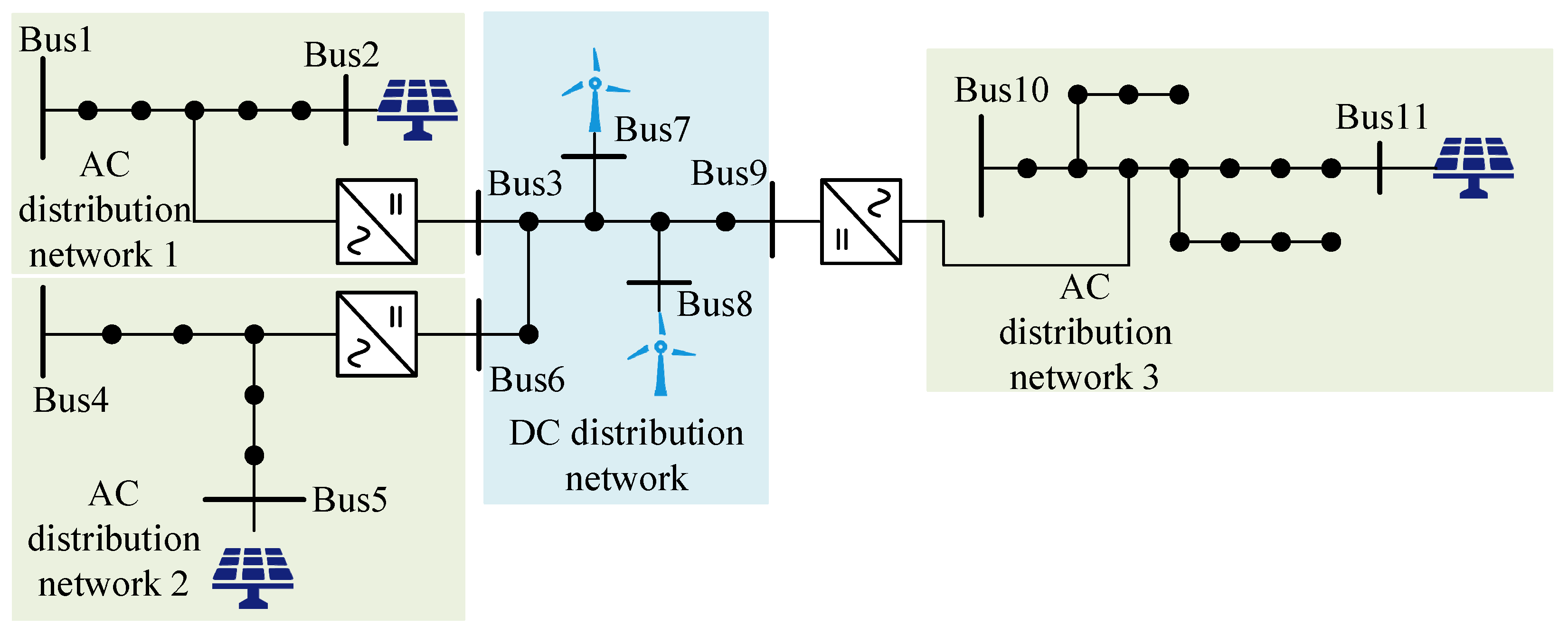
To verify the applicability of the proposed method in an AC/DC hybrid distribution network, this paper constructs the test system shown in Figure 1. The system consists of AC distribution network 1, AC distribution network 2, a DC distribution network, and AC distribution network 3. AC distribution network 1 and AC distribution network 2 are connected to the DC distribution network through converters, respectively. The DC distribution network is then interconnected with AC distribution network 3 through an interlinking converter, thus forming a typical AC/DC hybrid operating structure. On the AC side, three photovoltaic units are installed. Their output curves are taken from the actual photovoltaic generation data of Brussels, Flanders, and Wallonia in the public dataset of the Belgian Elia grid. On the DC side, two wind power units are installed. Their output curves are based on the actual wind power data of Flanders and Wallonia from the same dataset. The system load is constructed from the actual load data of the Belgian grid and is allocated according to the configuration ratio of AC and DC loads. After the overall configuration, the renewable energy penetration level of the system reaches 38%.

The operating risk of the main connection scheme of the AC/DC coupling station is evaluated under the typical daily operating condition in August. The risk indices include the risks of distribution line overload, AC/DC converter overload, and load supply interruption caused by faults of key equipment in the station.

5.2. Power Supply Reliability Assessment of AC/DC Hybrid Distribution Networks Based on Clustering of Typical Renewable Energy Scenarios

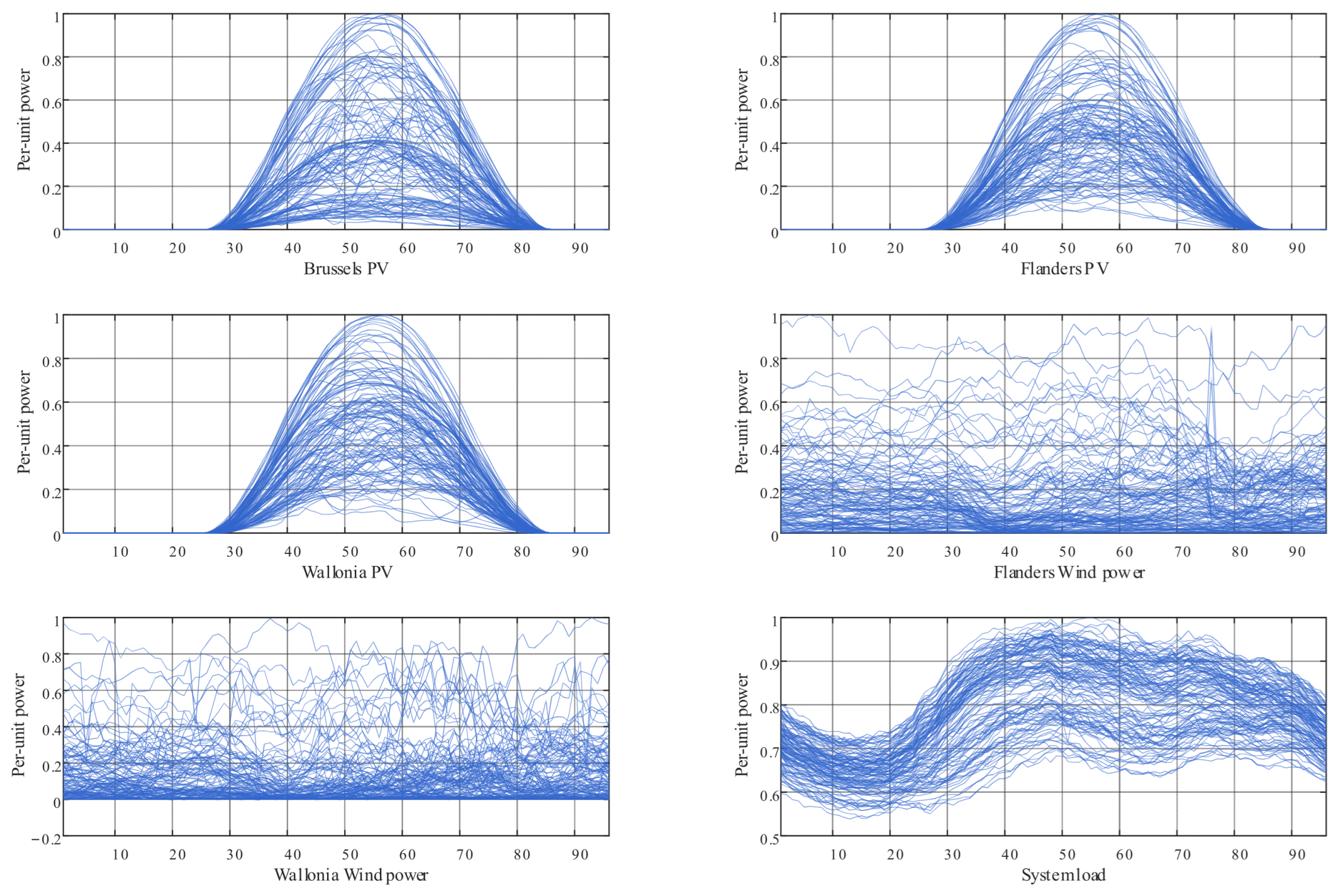
First, simulation-based verification is carried out to evaluate the effectiveness of the proposed clustering method for typical power grid operating scenarios with large-scale renewable energy integration, as well as the effectiveness of the power supply reliability assessment method for AC/DC hybrid distribution networks based on clustering of typical operating scenarios. To cluster the typical daily scenarios of renewable generation output and load demand in the AC/DC hybrid distribution network, this paper uses the actual variation curves of distributed photovoltaic power, wind power, and load demand in the Belgian power grid during August from 2021 to 2024. A total of 124 days of data are selected for clustering analysis. The per-unit curves of each renewable generation unit and the system load are shown in Figure 2.

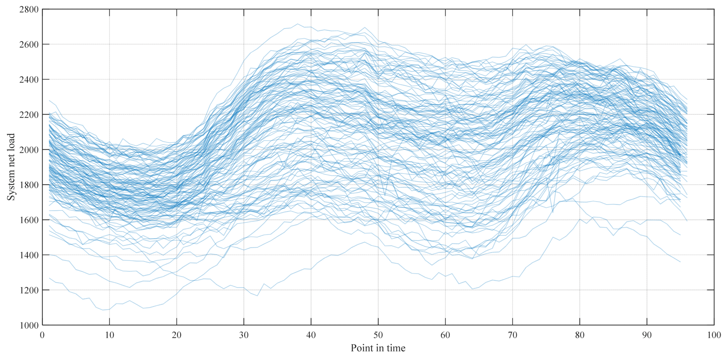
In constructing the AC/DC hybrid distribution network, the capacities of renewable generation units and loads are configured as follows. The capacities of the three photovoltaic units corresponding to the photovoltaic data of Brussels, Flanders, and Wallonia, and the capacities of the two wind power units corresponding to the wind power data of Flanders and Wallonia, are converted according to the rated capacity level of the system and then allocated to the AC side and the DC side, respectively. Meanwhile, the total load capacity of the system is kept unchanged and is distributed to each feeder according to the ratio of AC and DC loads. Based on the above configuration, Figure 2 shows the time-series variation characteristics of each system component. Figure 3 further presents the daily net load duration curves of the AC/DC hybrid distribution network.

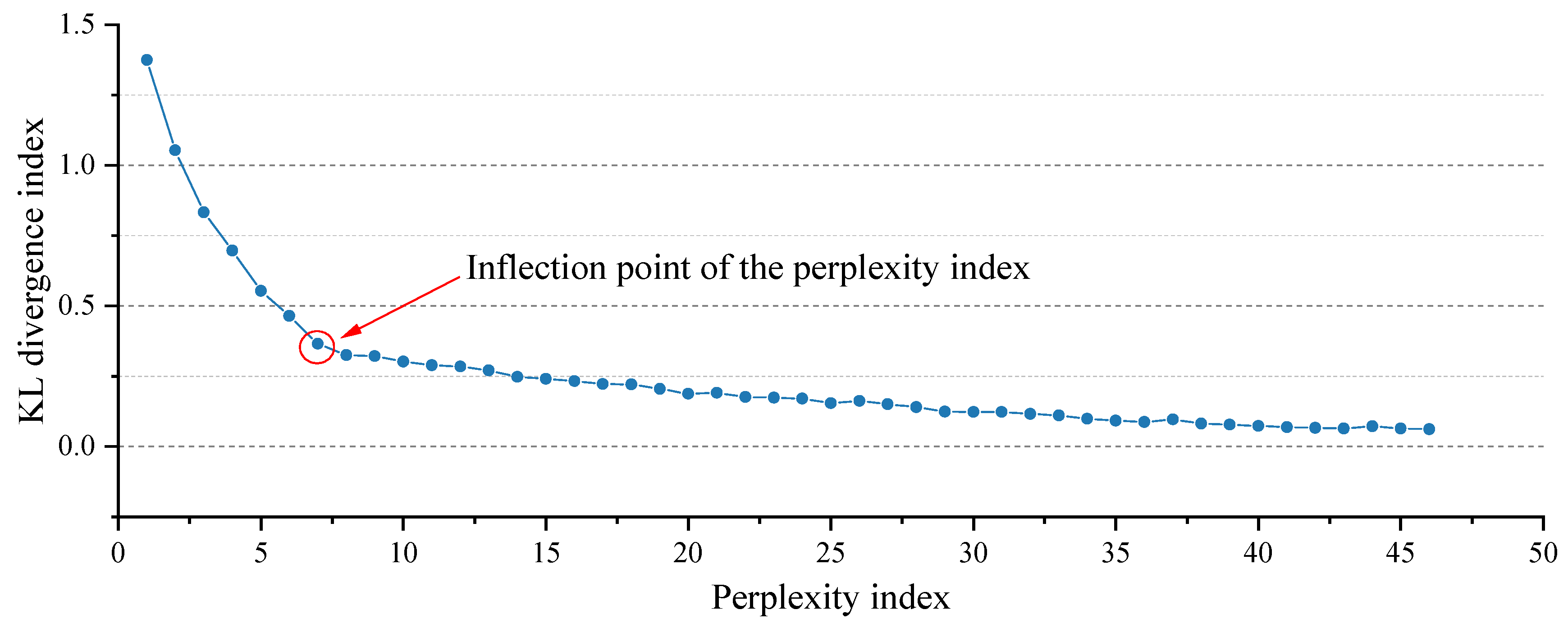
First, the improved t-SNE dimensionality reduction method proposed in this paper is used to reduce the dimensionality of the high-dimensional daily net load duration curves. Taking the KL divergence corresponding to different perplexity values as the objective, the curve of KL divergence versus perplexity is plotted. The result is shown in Figure 4.

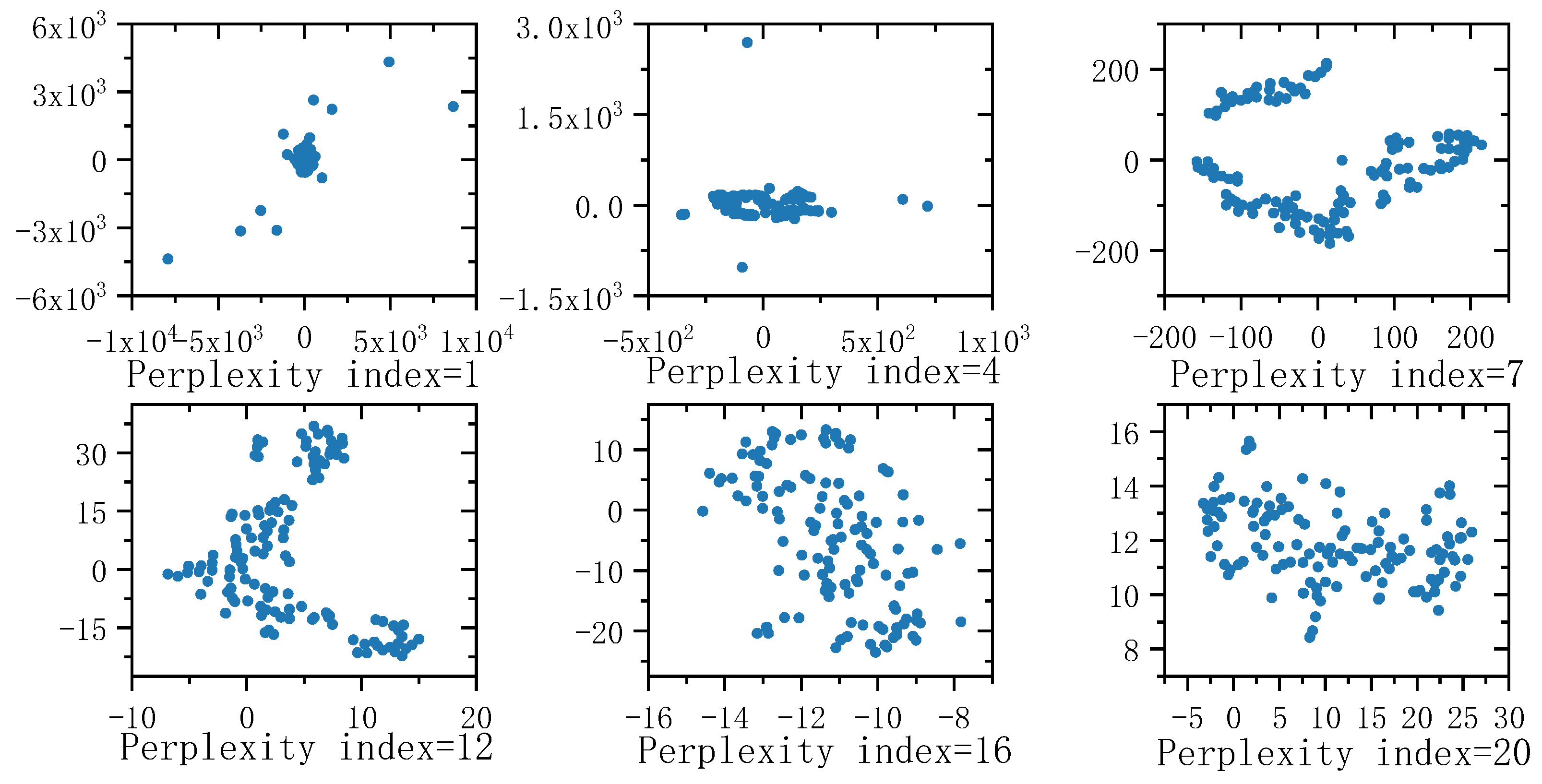
As shown in Figure 4, during the dimensionality reduction of the daily net load duration curves by the improved t-SNE algorithm, the KL divergence decreases continuously as the perplexity increases. This indicates that a larger perplexity leads to a higher similarity between the distribution of the dimension-reduced dataset and that of the original high-dimensional dataset, namely, the daily net load duration curves. The perplexity at the elbow point, i.e., 7, enables the dimension-reduced data to capture the global trend while preserving sufficient local structure. In this way, the reduced data can avoid being overly smooth or excessively fragmented, which would otherwise affect the subsequent clustering performance. The dimension-reduced results corresponding to different perplexity values are shown in Figure 5.

Figure 5 shows the distribution of data points in the dimension-reduced dataset in the two-dimensional space under different perplexity values. The horizontal and vertical coordinates only represent the positions of the dimension-reduced data points and have no actual physical meaning. As can be seen, when the perplexity is very small, the distribution of the dimension-reduced data points is relatively smooth, and the coordinate range is excessively large. This is not favorable for subsequent clustering. Similarly, when the perplexity is too large, the data points are concentrated within a very small region of the space, and the distribution becomes overly fragmented. This is also unfavorable for clustering. When the perplexity takes the elbow-point value of 7, the dimension-reduced data are distributed within an appropriate spatial range, and the data points do not exhibit a fragmented pattern. Therefore, this setting is suitable for clustering analysis. These results verify the effectiveness of the proposed t-SNE dimensionality reduction method based on the optimal KL divergence criterion.

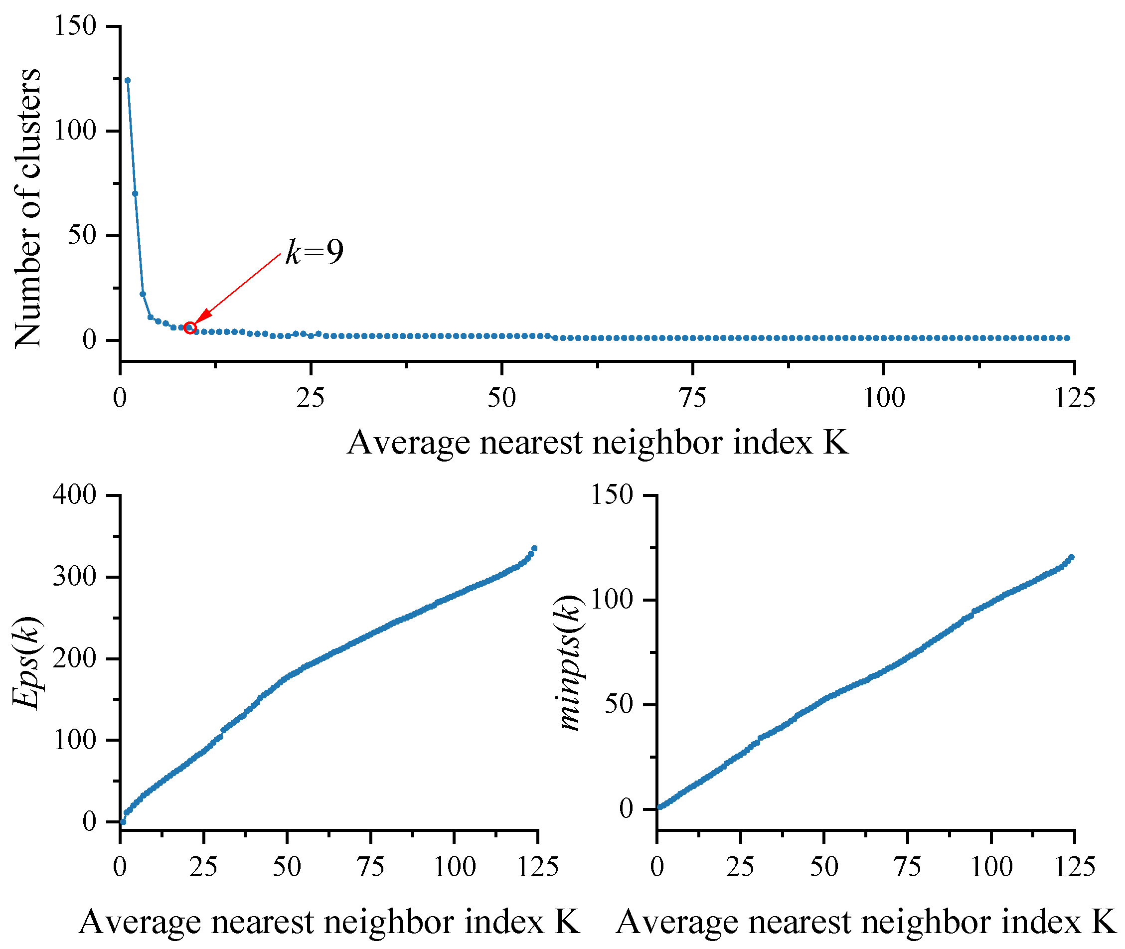
On the basis of dimensionality reduction of the high-dimensional daily net load duration curves, the improved DBSCAN clustering algorithm is further used to cluster the dimension-reduced data. By using the proposed method, the curve of the number of clusters versus the average k-nearest-neighbor distance coefficient is obtained, as shown in Figure 6.

As shown in Figure 6, the number of preliminary clusters in the dimension-reduced dataset decreases continuously as k increases. Each value of k corresponds to a pair of parameters, namely Eps(k) and MinPts(k). When k = 1, the number of clusters is 124. This indicates that, under the corresponding Eps(1), the neighborhood of each data point contains only the data point itself. When k is greater than 57, the number of clusters becomes 1. This means that all data points are assigned to a single cluster.

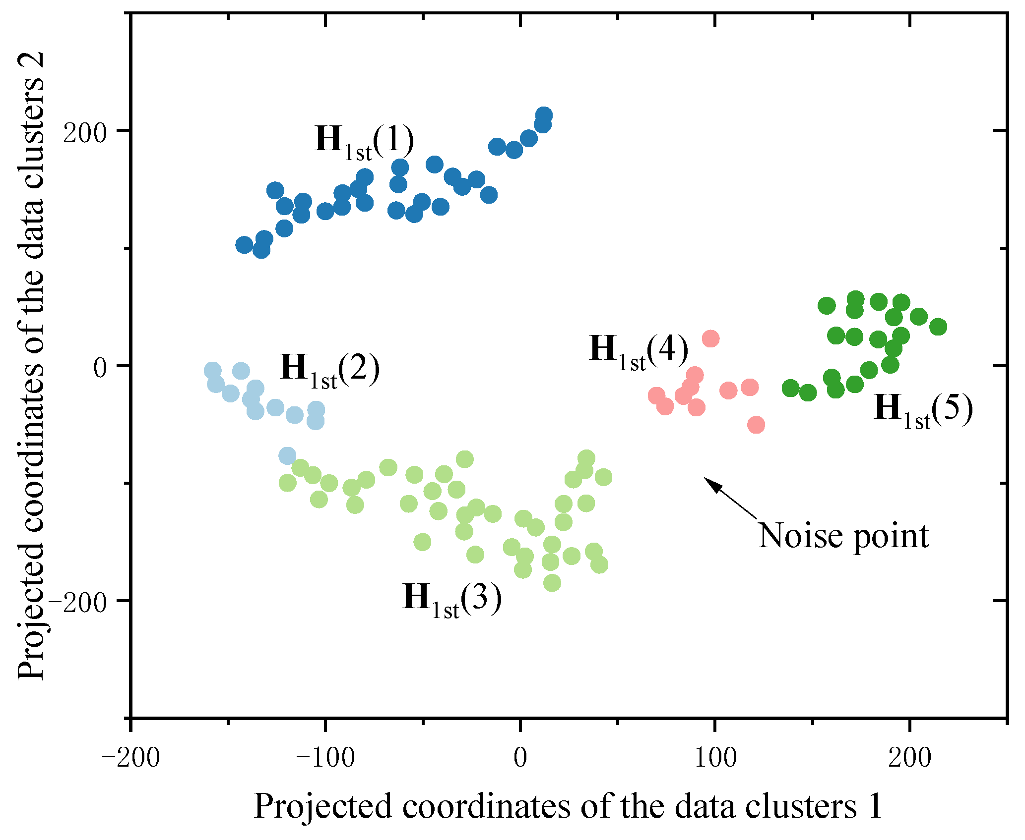
According to the criterion proposed in this paper, when k = 7, the same cluster number, namely 6, appears consecutively three times. Therefore, k = 9 is selected as the optimal average k-nearest-neighbor distance coefficient. The corresponding Eps(9) and MinPts(9) are 38.46 and 9, respectively. These values are then used as the input parameters of the DBSCAN clustering algorithm. The distribution of data point clusters after preliminary clustering is shown in Figure 7.

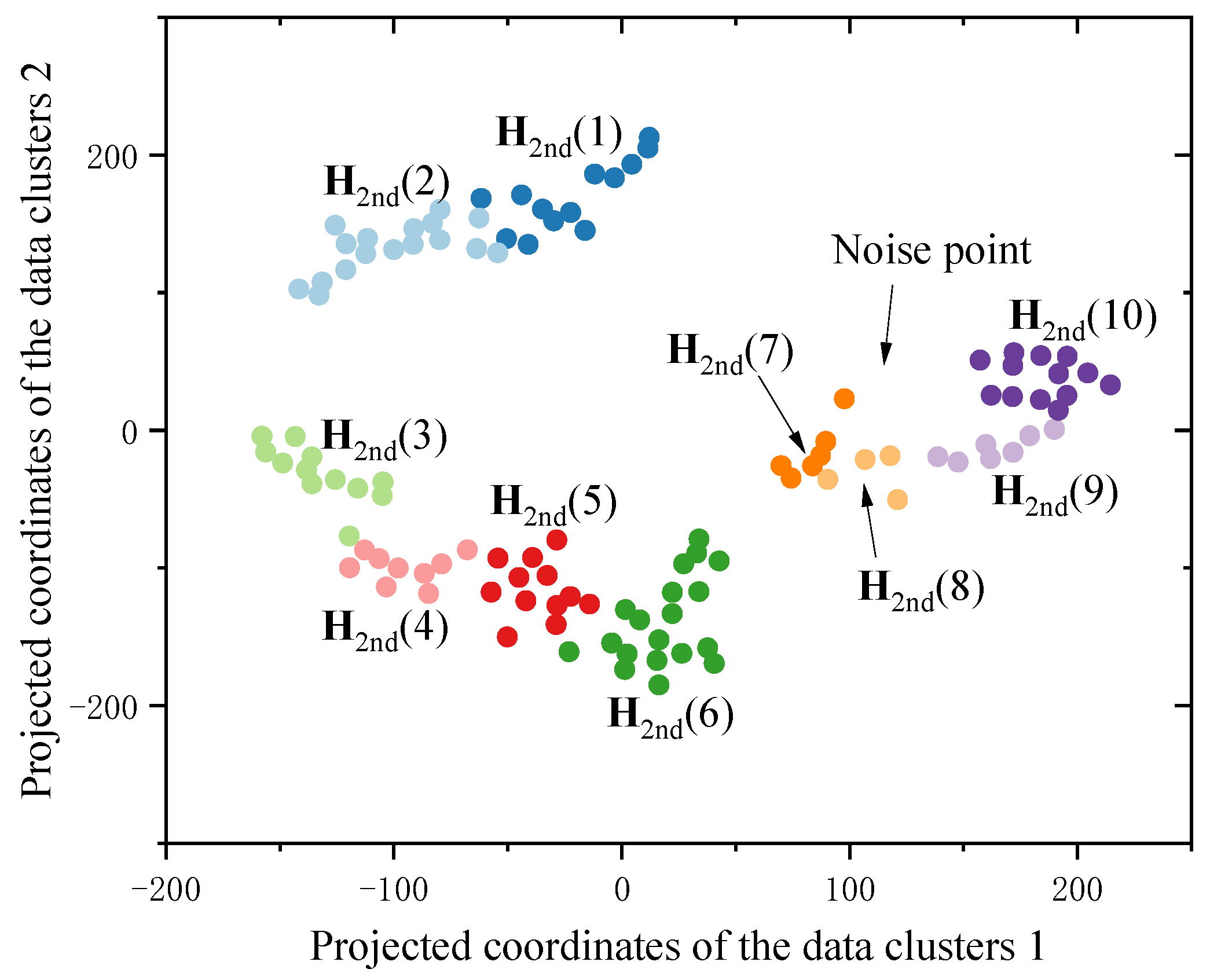
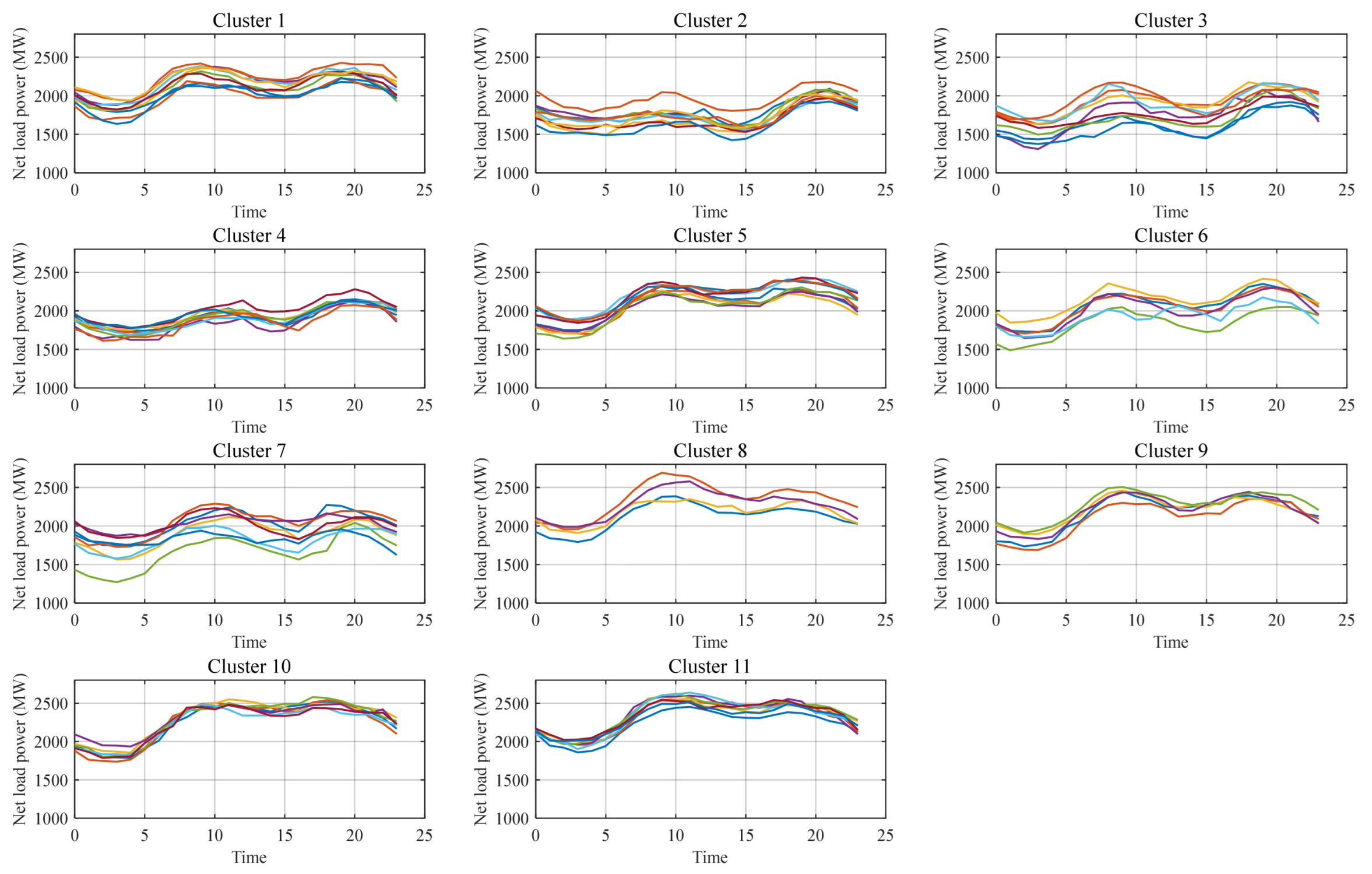
As shown in Figure 7, after preliminary clustering, the dimension-reduced dataset is divided into six clusters, including noise points, and the separation between clusters is clear. Clusters H_1st(1)~H_1st(5) contain 30, 12, 40, 10, and 20 data points, respectively, and there are 12 noise points. Based on the preliminary clustering results, the data in clusters H_1st(1)~H_1st(5) are further subjected to secondary clustering. The improved K-means algorithm described in Section 2 is adopted to perform optimal secondary clustering for each sub-cluster. The secondary clustering results are organized as shown in Figure 8, and the corresponding daily net load duration curves within each cluster are presented as shown in Figure 9.

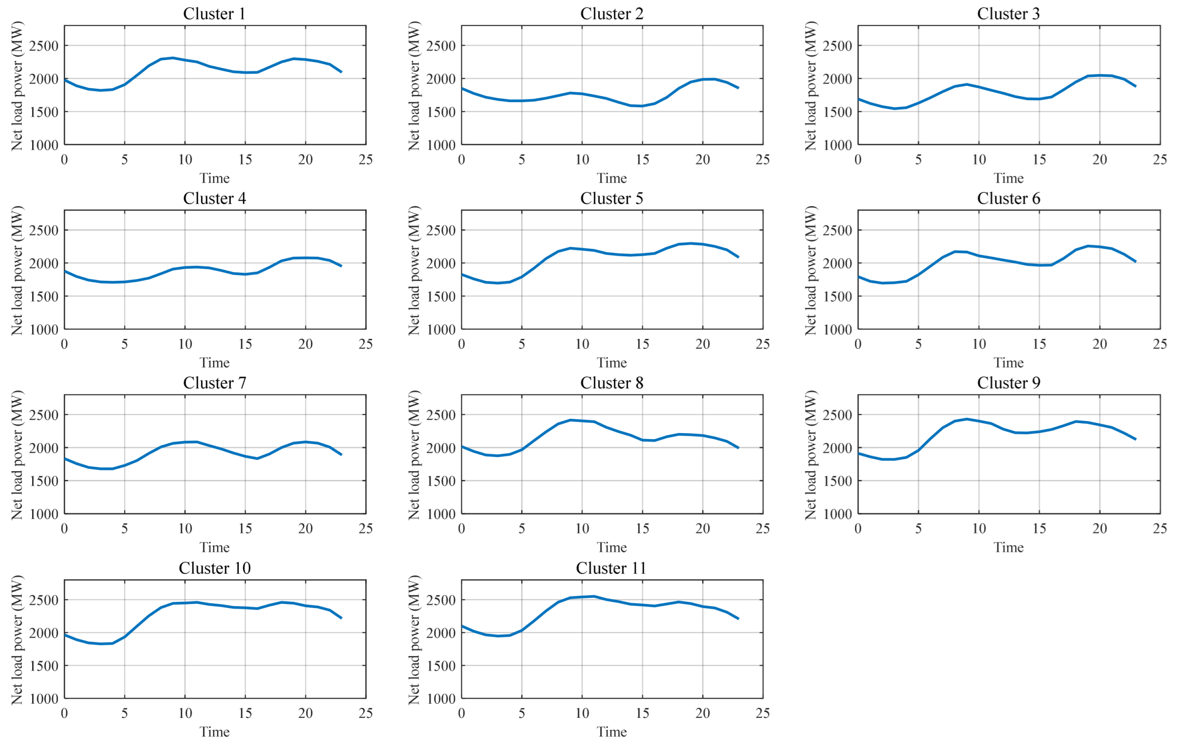
As shown in Figure 9, after secondary clustering by the improved K-means algorithm proposed in this paper, the original data are further divided into 11 clusters, including noise points. The high-dimensional daily net load duration curves corresponding to the data points in each secondary cluster are plotted in the same coordinate system. In this way, the 124 daily net load duration curves shown in Figure 3 can be decomposed into 11 types of daily net load duration curves, as shown in Figure 9. It can be observed that the clustering results exhibit high intra-cluster compactness and clear inter-cluster differences. The clustered results can effectively distinguish the overall structure while preserving the local characteristics of the daily net load duration curves.

To evaluate the clustering performance of the proposed method, the following four methods are used to cluster the daily net load duration curves shown in Figure 3.

Method 1: Conventional K-means algorithm;

Method 2: t-SNE + DBSCAN algorithm;

Method 3: Fuzzy c-means (FCM) clustering algorithm;

Method 4: The proposed improved t-SNE-DBSCAN–K-means clustering algorithm.

In this paper, the clustering of daily net load duration curves based on the above algorithms is implemented in MATLAB 2022b. The DB index is used to evaluate the quality of the clustering results. The calculated results are presented in

Table 1. Quality comparison of clustering results obtained by different algorithms.

Clustering Method	Method 1	Method 2	Method 3	Method 4
Number of clusters	11	6	8	11
DB index	1.688	0.681	0.766	0.532

.

Since the conventional K-means algorithm and the conventional DBSCAN algorithm require clustering parameters to be specified manually, the number of clusters in the K-means algorithm is set to be the same as that obtained by the proposed method. The input parameters of the DBSCAN algorithm are set to 38.46 and 9. From the clustering results, the proposed method yields the smallest DB index. This indicates that, while maintaining high intra-cluster compactness, it also achieves the largest inter-cluster separation, and thus provides the best clustering performance. In addition, Method 1 has a relatively large DB index, which indicates that the conventional K-means algorithm is not suitable for direct clustering of high-dimensional data. The clustering result of Method 2 corresponds to the preliminary clustering result shown in Figure 7, whereas the proposed method further improves the clustering quality through secondary clustering. Compared with Methods 1 to 3, the proposed clustering method reduces the DB index by 68%, 22%, and 31%, respectively.

To further verify the effectiveness of the proposed method in the power supply reliability assessment of the AC/DC hybrid distribution network at the substation level, the final cluster centroids are used to extract the corresponding representative daily net load duration curves. These curves are organized into 11 typical daily net load duration curves of the system, as shown in Figure 10. The probabilities of the typical daily operating scenarios corresponding to each cluster are listed in

Table 2. Occurrence probabilities of the typical daily scenarios corresponding to each cluster.

Typical Day	Occurrence Probability	Typical Day	Occurrence Probability
Cluster 1	9.68%	Cluster 2	13.71%
Cluster 3	10.48%	Cluster 4	9.68%
Cluster 5	15.32%	Cluster 6	7.26%
Cluster 7	9.68%	Cluster 8	3.23%
Cluster 9	4.84%	Cluster 10	5.65%
Cluster 11	10.48%

.

The power supply reliability of the AC/DC hybrid distribution network at the substation level is evaluated under each typical daily operating scenario corresponding to each cluster. Then, the risk indices are weighted according to Table 2. The final power supply reliability indices are listed in

Table 3. Comparison of power supply reliability indices obtained by the typical-scenario-based method and the full time-series simulation method.

Index	Typical-Scenario-Based Method	Index	Full Time-Series Simulation
PLC	0.4998%	PLC	0.5132%
EFLC	0.001301 times/day	EFLC	0.001381 times/day
EENS	4.6623 MWh/day	EENS	4.865 MWh/day
Computation time	968 s	Computation time	8513 s

. To verify the effectiveness of the proposed method, the table also gives the power supply reliability indices obtained from full time-series simulation for comparison.

The results show that the difference between the full time-series method and the typical daily operating scenario method proposed in this paper is within an acceptable range in the power supply reliability assessment of the AC/DC hybrid distribution network at the substation level. The relative errors of PLC, EFLC, and EENS are 2.61%, 5.79%, and 4.17%, respectively. This may be because, during the formation of the typical daily load curves, the system net load values at high-net-load periods, which have a greater impact on the risk indices, are reduced. Such an error is difficult to avoid in risk assessment based on typical scenarios, but it is acceptable within the allowable accuracy range. In terms of computation time, compared with full time-series simulation, the power supply reliability assessment method based on the proposed clustering of typical operating scenarios improves the computational efficiency by about 8.8 times. This significantly improves the computational efficiency. These results indicate that the proposed method can greatly reduce computation time while maintaining acceptable accuracy.

6. Conclusions

Large-scale integration of renewable energy sources significantly changes the operating characteristics of power systems. The volatility and randomness of renewable generation also bring greater challenges to power supply reliability assessment. To address the problem of power supply reliability assessment under large-scale renewable energy integration, this paper proposes a complete framework for typical operating scenario clustering and risk assessment. First, based on an analysis of power system operating characteristics, the daily net load duration curve is selected as the feature variable for reliability assessment, so as to characterize the typical operating scenarios of power systems with high renewable penetration. Second, in the dimensionality reduction stage, an improved t-SNE algorithm based on the optimal KL divergence criterion is proposed. This method optimizes the low-dimensional embedding process of high-dimensional time-series data and improves the dimensionality reduction accuracy of operating curves. Further, in the clustering stage, an adaptive DBSCAN parameter optimization method based on the k-nearest-neighbor curve is proposed to automatically determine Eps and MinPts. In addition, an SC-DB multi-objective optimization model based on the entropy weight method is established to optimize the value of K for secondary K-means clustering. On this basis, a hybrid t-SNE-DBSCAN–K-means clustering algorithm is constructed, which significantly improves the clustering quality of high-dimensional time-series curves. Finally, a power supply reliability assessment method for the AC/DC hybrid distribution network at the substation level is developed based on clustering of typical renewable energy scenarios. This method provides an effective quantitative analysis tool for the power supply reliability assessment of AC/DC hybrid distribution networks with large-scale renewable energy integration in the context of new-type power systems. By combining the improved dimensionality reduction algorithm with the optimized two-stage clustering strategy, the proposed method achieves high-accuracy extraction of operating scenario features and provides a theoretical basis and technical support for subsequent risk assessment of AC/DC hybrid distribution networks. The case study results show that:

(1) The proposed t-SNE-DBSCAN–K-means method for typical operating scenario clustering has significant advantages in clustering quality. Its DB index is improved by at least 22% compared with conventional clustering methods. This verifies the superiority of the proposed algorithm in extracting operating scenario features.

(2) In terms of risk assessment accuracy, the maximum relative error between the power supply reliability assessment results based on typical daily scenarios and those obtained by full time-series simulation is less than 6%. At the same time, the computational efficiency is improved by 8.8 times. Therefore, the proposed method achieves a good balance between accuracy and efficiency. These results demonstrate that the proposed method can greatly reduce computational cost while maintaining an accuracy acceptable for engineering applications. It therefore provides an efficient and reliable solution for large-scale risk assessment in the context of new-type power systems.

References

1. Li, Z.; Tan, H.; Zhang, Y.; Xu, M.; Zhang, L.; Li, K.; Tian, R.; Liu, C. Optimal Splitting Sections Searching Method for Power Systems with Grid-Forming Wind Turbines Based on Branch Transient Potential Energy. Energies 2026, 19, 1496. [Google Scholar] [CrossRef]
2. Liu, C.; Li, P.; Liu, G.; Yang, H.; Sun, C. Performance and Robustness Evaluation of the Resonance Suppression Strategy for the Photovoltaic Grid-Connected System Based on the Entropy Weight Method. Energies 2026, 19, 1886. [Google Scholar] [CrossRef]
3. Tang, M.; Li, R.; Zhang, R.; Yang, S. Research on New Electric Power System Risk Assessment Based on Cloud Model. Sustainability 2024, 16, 2014. [Google Scholar] [CrossRef]
4. Wang, Z.; Bu, S.; Wen, J.; Huang, C. A Comprehensive Review on Uncertainty Modeling Methods in Modern Power Systems. Int. J. Electr. Power Energy Syst. 2025, 166, 110534. [Google Scholar] [CrossRef]
5. Hu, B.; Xie, K.; Shao, C.; Pan, C.; Lin, C.; Zhao, Y. Commentary on Risk of New Power System under Goals of Carbon Emission Peak and Carbon Neutrality: Characteristics, Indices and Assessment Methods. Autom. Electr. Power Syst. 2023, 47, 1–15. [Google Scholar] [CrossRef]
6. Li, K.; Duan, P.; Xue, Q.; Cheng, Y.; Hua, J.; Chen, J.; Guo, P. Enhancing Reliability Assessment in Distributed Generation Networks: Incorporating Dynamic Correlation of Wind-Solar Power Output Uncertainty. Sustain. Energy Grids Netw. 2024, 39, 101505. [Google Scholar] [CrossRef]
7. Wen, S.; Dai, D.; Xie, S.; He, Y. Multi-Dimensional Reliability Assessment of Distribution Network under Renewable Energy Installation and Load Installation. Electronics 2025, 14, 4378. [Google Scholar] [CrossRef]
8. Qu, Z.; Zhang, Z.; Qu, N.; Zhou, Y.; Li, Y.; Jiang, T.; Li, M.; Long, C. Extraction of Typical Operating Scenarios of New Power System Based on Deep Time Series Aggregation. CAAI Trans. Intell. Technol. 2025, 10, 283–299. [Google Scholar] [CrossRef]
9. Zhang, Z.; Qu, X.; Wang, Q. A Probabilistic Clustering Method for Annual Typical-Day of Power Systems Considering Supply-Demand Ratio of Frequency Regulation. Trans. China Electrotech. Soc. 2025, 20251518. [Google Scholar] [CrossRef]
10. Safari, N.; Chung, C.Y.; Price, G.C.D. Novel Multi-Step Short-Term Wind Power Prediction Framework Based on Chaotic Time Series Analysis and Singular Spectrum Analysis. IEEE Trans. Power Syst. 2018, 33, 590–601. [Google Scholar] [CrossRef]
11. Yang, X.; Yang, Y.; Liu, Y.; Deng, Z. A Reliability Assessment Approach for Electric Power Systems Considering Wind Power Uncertainty. IEEE Access 2020, 8, 12467–12478. [Google Scholar] [CrossRef]
12. Li, J.; Lan, F.; Wei, H. A Scenario Optimal Reduction Method for Wind Power Time Series. IEEE Trans. Power Syst. 2016, 31, 1657–1658. [Google Scholar] [CrossRef]
13. Xiao, L.; Muttaqi, K.M.; Agalgaonkar, A.P. Reliability Assessment of Modern Distribution Networks Embedded with Renewable and Distributed Resources. Electr. Power Syst. Res. 2022, 212, 108374. [Google Scholar] [CrossRef]
14. Xin, K.; Ma, Q.; Xu, Q.; Wang, Z.; Liu, Y. Wind Power Output Sequence Scenario Generation Method Based on Monthly Division and Specified Day Type. Autom. Electr. Power Syst. 2023, 47, 151–161. [Google Scholar]
15. Li, Z.; Peng, X.; Cui, W.; Xu, Y.; Liu, J.; Yuan, H.; Lai, C.S.; Lai, L.L. A Novel Scenario Generation Method of Renewable Energy Using Improved VAEGAN with Controllable Interpretable Features. Appl. Energy 2024, 363, 122905. [Google Scholar] [CrossRef]
16. Li, H.; Yu, H.; Liu, Z.; Li, F.; Wu, X.; Cao, B.; Zhang, C.; Liu, D. Long-Term Scenario Generation of Renewable Energy Generation Using Attention-Based Conditional Generative Adversarial Networks. IET Energy Convers. Econ. 2024, 5, 15–27. [Google Scholar] [CrossRef]
17. Michalakopoulos, V.; Sarmas, E.; Papias, I.; Skaloumpakas, P.; Marinakis, V.; Doukas, H. A Machine Learning-Based Framework for Clustering Residential Electricity Load Profiles to Enhance Demand Response Programs. Appl. Energy 2024, 361, 122943. [Google Scholar] [CrossRef]
18. Kim, J.; Song, K.; Lee, G.; Lee, S. Time-Series Data Clustering with Load-Shape Preservation for Identifying Residential Energy Consumption Behaviors. Energy Build. 2024, 311, 114130. [Google Scholar] [CrossRef]
19. Ding, M.; Xie, J.; Liu, X.; Shi, W. The Generation Method and Application of Wind Resources/Load Typical Scenario Set for Evaluation of Wind Power Grid Integration. Proc. CSEE 2016, 36, 4064–4072. [Google Scholar] [CrossRef]
20. Cao, Y.; Li, P.; Yuan, Y.; Zhang, X.; Guo, S.; Zhang, C.F. Analysis on Accommodating Capability of Renewable Energy and Assessment on Low-Carbon Benefits Based on Time-Sequence Simulation. Autom. Electr. Power Syst. 2014, 38, 60–66. [Google Scholar] [CrossRef]
21. Kirchner-Bossi, N.; García-Herrera, R.; Prieto, L.; Trigo, R.M. A Long-Term Perspective of Wind Power Output Variability. Int. J. Climatol. 2015, 35, 2635–2646. [Google Scholar] [CrossRef]
22. Ye, J.; Zhu, J.; Lu, Q.; Li, T.S.; Chang, S.Q.; Wang, Q.G. A Fault Detection Method of Photovoltaic Power Station Based on Improved DBSCAN Clustering Algorithm. J. Guangxi Univ. Nat. Sci. Ed. 2019, 44, 440–447. [Google Scholar] [CrossRef]
23. Huang, Y.F.; He, W.; Wu, G.Q.; Li, D. Research on Photovoltaic Power Prediction Based on K-Means++ and LSTM Network. Electr. Autom. 2020, 42, 25–27, 34. [Google Scholar]
24. Lou, J.; Cao, H.; Zheng, H.; Xiao, J. Anomaly Monitoring of Power Characteristic of Wind Turbine Based on Multi-Dimensional Clustering Method. Adv. Sci. Technol. Lett. 2016, 139, 433–438. [Google Scholar]
25. Fang, M.; Sun, Z.; Zhou, G.; Xie, F.; Wang, P. Typical Power Daily Load Classification Based on Fuzzy C-Means Clustering Algorithm. North China Electr. Power 2016, 11, 15–19. [Google Scholar]
26. Luo, Y.; Peng, H.; Cheng, T.; Luo, Y.; Liu, X.; Huang, D. Domain Knowledge-Enhanced Graph Reinforcement Learning Method for Volt/Var Control in Distribution Networks. Appl. Energy 2025, 398, 126409. [Google Scholar] [CrossRef]
Figure 1. Schematic diagram of the AC/DC hybrid distribution network system.
Energies 19 02549 g001
Figure 2. Time-series variation curves of renewable energy stations and system load.
Energies 19 02549 g002
Figure 3. Daily net load duration curves of the AC/DC hybrid distribution network.
Energies 19 02549 g003
Figure 4. Variation curve of the KL divergence with perplexity in t-SNE dimensionality reduction.
Energies 19 02549 g004
Figure 5. Distribution of dimension-reduced data under different perplexity values.
Energies 19 02549 g005
Figure 6. Variation in the number of clusters, Eps(k), and MinPts(k) with the average k-nearest-neighbor distance coefficient.
Energies 19 02549 g006
Figure 7. Preliminary clustering results.
Energies 19 02549 g007
Figure 8. Secondary clustering results.
Energies 19 02549 g008
Figure 9. Schematic diagram of the daily net load duration curves corresponding to each cluster.
Energies 19 02549 g009
Figure 10. Typical daily net load duration curves.
Energies 19 02549 g010