Predictive Models for Renewable Energy Generation and Demand in Smart Cities: A Spatio-Temporal Framework

Abstract

The accelerating pace of urbanization and the pressing need for sustainability have compelled cities worldwide to integrate renewable energy into their infrastructure. While solar, wind, and hydro sources offer cleaner alternatives to fossil fuels, their inherent variability creates challenges in maintaining balance between supply and demand in urban energy systems. Traditional statistical forecasting methods are often inadequate for capturing the nonlinear, weather-driven dynamics of renewables, highlighting the need for advanced artificial intelligence (AI) approaches that deliver both accuracy and interpretability. This paper proposes a spatio-temporal framework for smart city energy management that combines a Convolutional Neural Network with Long Short-Term Memory (CNN-LSTM) for renewable energy generation forecasting, a Gradient Boosting Machine (GBM) for urban demand prediction, and Particle Swarm Optimization (PSO) for cost-efficient energy allocation. The framework was first validated using Spain’s national hourly energy dataset (2015–2018). To rigorously test its generalizability, the methodology was further validated on a separate dataset for the German energy market (2019–2022), proving its robustness across different geographical and meteorological contexts. Results indicate strong predictive performance, with solar generation achieving a 99.03% R² score, wind 96.46%, hydro 93.02%, and demand forecasting 91.56%. PSO further minimized system costs, reduced reliance on fossil-fuel generation by 18.2%, and improved overall grid efficiency by 12%. These findings underscore the potential of AI frameworks to enhance reliability and reduce operational costs.

1. Introduction

The global energy landscape is undergoing a rapid transformation as cities strive to address the dual challenges of urbanization and climate change. With more than 68% of the world’s population expected to live in cities by 2050, energy demand is projected to rise significantly, placing unprecedented strain on urban infrastructure [1]. Renewable energy sources such as solar, wind, and hydro have emerged as sustainable alternatives to fossil fuels, offering the potential to reduce greenhouse gas emissions and enhance energy security. However, their inherent variability, driven by weather conditions and seasonal cycles, complicates integration into smart city energy systems. Sudden changes in cloud cover, wind speed, or precipitation can lead to fluctuations in generation, resulting in mismatches between supply and demand.

Smart cities, which leverage Internet of Things (IoT) devices, big data, and artificial intelligence (AI), present new opportunities to overcome these challenges. By analyzing real-time or historical datasets. AI-driven models can forecast both energy generation and demand, enabling proactive and efficient energy management. The importance of predictive modeling is particularly evident in ambitious national projects such as Saudi Arabia’s Vision 2030 initiatives, including NEOM and The Line, which emphasize renewable energy as the backbone of urban development [2]. In such contexts, advanced predictive frameworks not only ensure energy reliability but also support broader goals of sustainability.

Despite advancements in renewable forecasting, existing models face limitations. Some statistical approaches are not effective to capture nonlinear relationships, while traditional machine learning models such as Support Vector Machines and Random Forests struggle with high-dimensional and time-dependent data. Deep learning techniques like LSTM have shown promise in capturing sequential dependencies but often overlook spatial variability. Conversely, convolutional models such as CNN excel at spatial feature extraction yet lack temporal modeling capabilities. In demand forecasting, many approaches achieve numerical accuracy but limit their usefulness in policymaking and operational decision-making. Moreover, forecasting alone [3] is insufficient without efficient allocation strategies that minimize costs and balance resources across renewable and non-renewable sources. 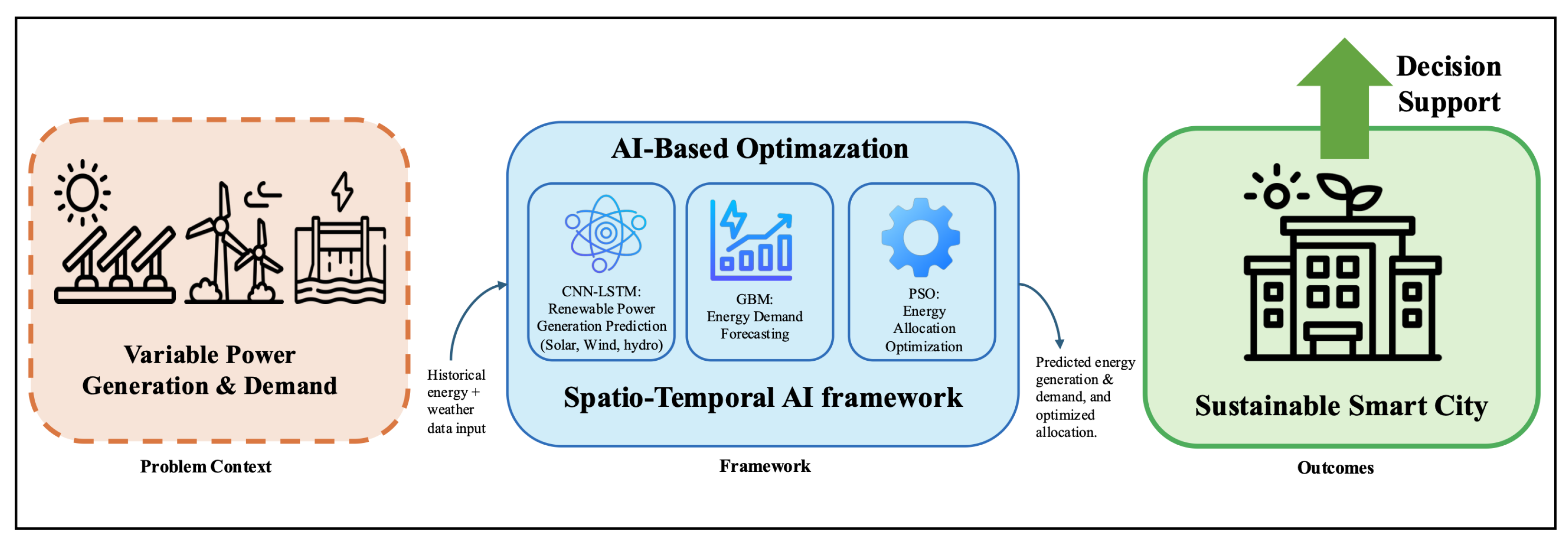To address these limitations, Figure 1 illustrates the proposed framework, which integrates spatio-temporal forecasting with optimization to ensure efficient energy management.

Aim and Objectives

This study aims to employ artificial intelligence (AI) techniques to design a spatio-temporal framework capable of forecasting renewable energy generation and urban energy demand while optimizing resource allocation in smart cities.

This goal is addressed through the following objectives:

• Develop a CNN-LSTM-based model to accurately predict solar, wind, and hydro energy production using weather data and historical records.
• Create an interpretable model, using Gradient Boosting Machines (GBMs), to predict energy consumption.
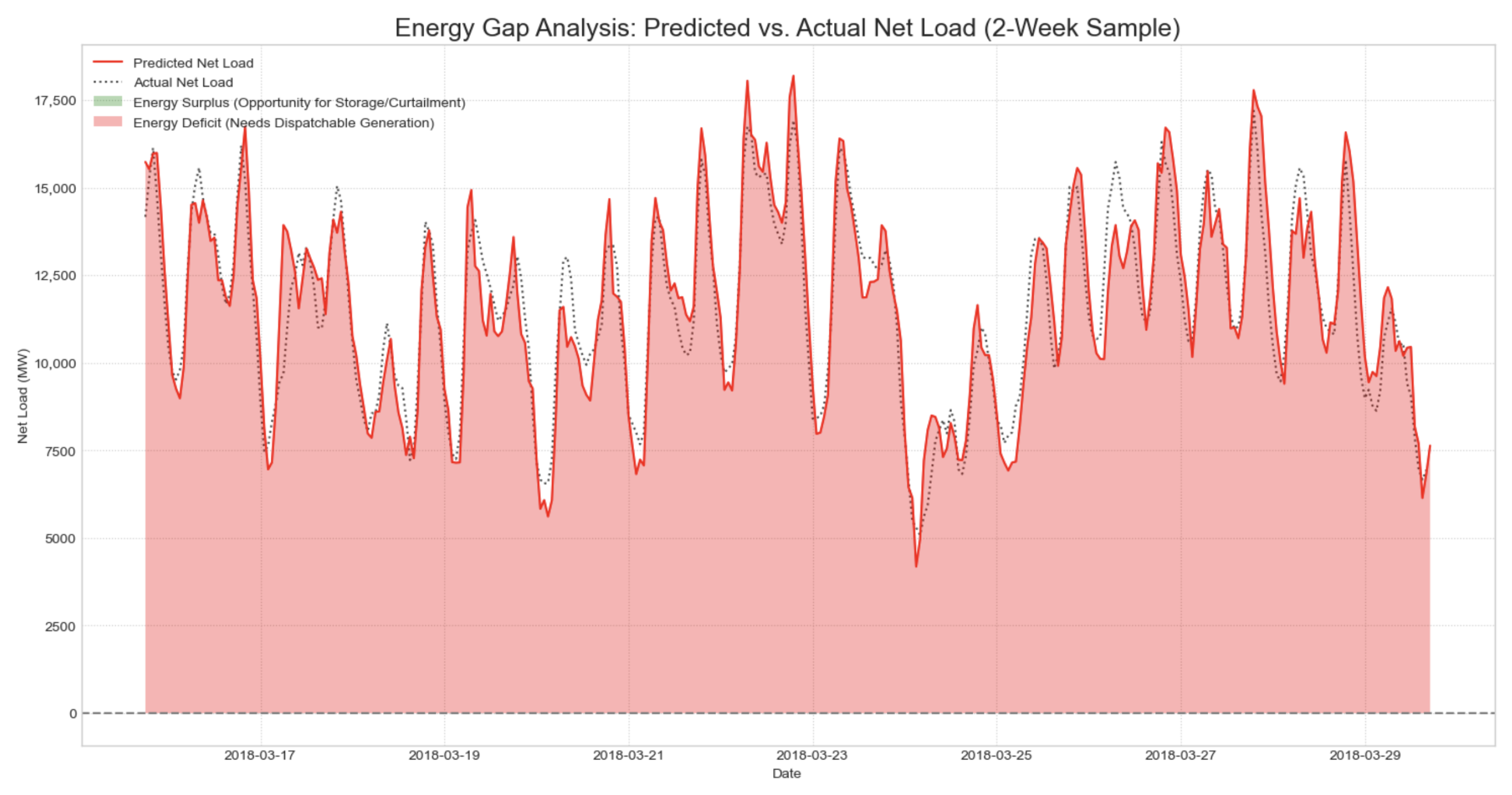
• Integrate and analyze the performance of prediction models by evaluating the combined generation and demand prediction framework to identify gaps and ensure efficient energy management.
• Design an optimization model powered by Particle Swarm Optimization (PSO) to allocate energy resources efficiently, minimizing losses and maximizing renewable energy utilization in smart cities.

2. Related Work

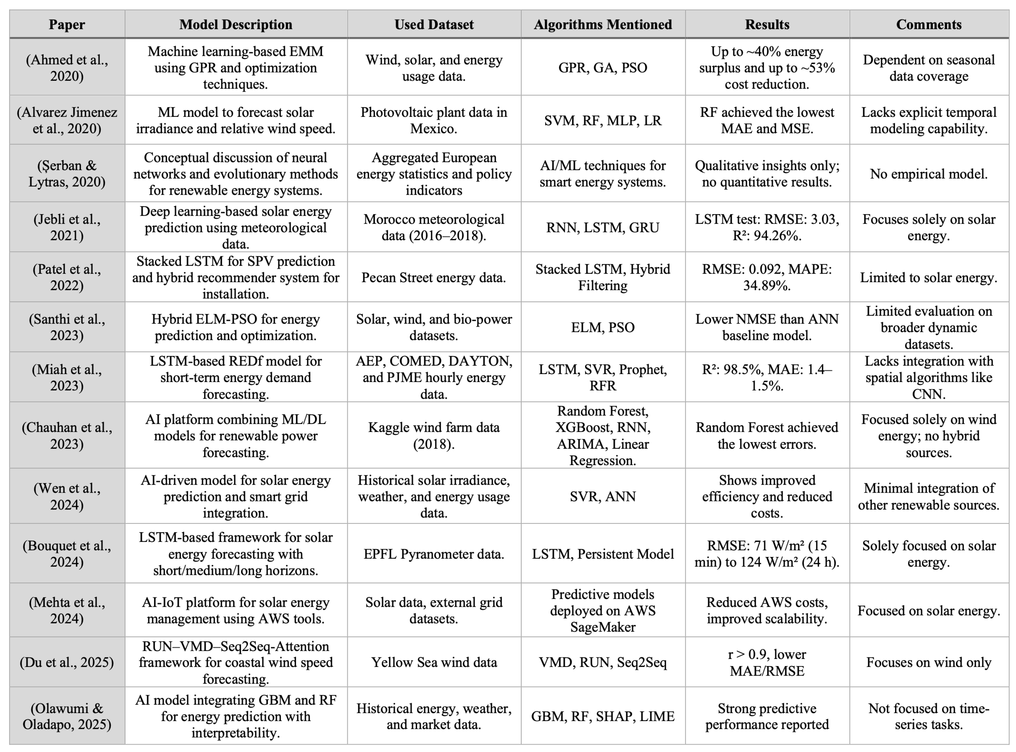
The integration of renewable energy in smart cities has been the subject of extensive research, with particular focus on forecasting variability and optimizing distribution. Studies from 2020 onward have increasingly adopted AI-based approaches to address limitations of traditional statistical models. This section provides a concise overview of related work from previous studies to address the challenges or gaps. A variety of papers were analyzed by comparative analysis that critically evaluates the reviewed studies to uncover key insights and research gaps. The summary is illustrated in the Figure 2.

The reviewed papers [4,5,6,7,8,9,10,11,12,13,14,15,16] exhibit notable differences in scope and modeling choices. This paper [4] proposes a GPR-based energy-management model for smart grids that jointly considers wind, solar, and load data, whereas paper [5] uses classical ML (SVM, RF, MLP, LR) to forecast solar irradiance and relative wind speed for a single PV plant. Paper [6] provides a high-level AI framework for smart renewable-energy infrastructures in Europe, focusing on conceptual indicators rather than empirical models. Several studies concentrate exclusively on solar prediction using deep learning, including RNN/LSTM/GRU models on Moroccan meteorological data [7], a stacked LSTM with a hybrid recommender for SPV installation using Pecan Street data [8], and SVR/ANN models for AI-driven solar generation and smart-grid integration [12]. Paper [13] designs an LSTM-based forecasting framework over multiple horizons using EPFL pyranometer measurements, while paper [14] focuses on an AI–IoT energy management platform deployed on AWS. Other works target broader renewable portfolios or demand includes paper [9] that employ a hybrid ELM–PSO scheme over solar, wind, and bio-power datasets, paper [10] that introduces an LSTM-based REDf model for short-term energy demand using multiple utility datasets, paper [11] that develops a cloud-based forecasting platform combining tree-based and time-series models on Kaggle wind-farm data, paper [15] that couples VMD, RUN, and Seq2Seq architectures for coastal wind-speed forecasting and paper [16] studies the GBM/RF-based predictive models for sustainability metrics with SHAP/LIME-based interpretability.

A review of these studies reveals persistent multiple research gaps. Many models focus on a single dominant source—typically solar [7,8,12,13,14] or wind [11,15]—while only a few consider multiple energy carriers or jointly model demand and generation [4,9,10,16]. Hybrid or advanced architectures such as ELM–PSO and RUN–VMD–Seq2Seq [9,15] address specific optimization or noise-decomposition challenges, but most approaches still rely on standard LSTM or tree-based baselines [7,8,10,11,13,16]. None of the works [4,5,6,7,8,9,10,11,12,13,14,15,16] explicitly integrates spatial dependencies through CNN-based spatio-temporal modeling; spatial variation is typically handled only via site-specific time series (e.g., single plants, districts, or coastal stations). Interpretability techniques such as SHAP and LIME are used systematically only in [16], leaving most deep and ensemble models as black boxes. Finally, although several papers touch on smart-grid or cloud-based deployment [4,6,11,14], real-time IoT-enabled integration of multi-source renewable forecasting with grid-level decision support remains limited, motivating the need for more holistic spatio-temporal and interpretable frameworks.

Furthermore, the field of AI-driven energy forecasting is rapidly evolving. While our proposed CNN-LSTM architecture is a robust and widely used hybrid model, recent years have seen the rise in alternative state-of-the-art approaches. Transformer-based architectures, for example, have shown significant promise in capturing long-range temporal dependencies in time-series forecasting [17,18]. Concurrently, Graph Neural Networks (GNNs) are being increasingly explored to model the inherent graph structure of power grids, offering a more explicit way to handle spatial relationships in regional forecasting [19,20]. Other recent advancements include novel hybrid models combining deep learning with advanced decomposition techniques [21], a growing focus on probabilistic forecasting to quantify uncertainty [22], and the application of physics-informed machine learning (PIML) to integrate physical laws into the modeling process [23]. Alternative optimization strategies, such as deep reinforcement learning, are also gaining traction for real-time energy management [24]. While a full comparative analysis is beyond the scope of this study (as discussed in Section 5.2), situating our work in this context highlights that our framework represents a practical and validated end-to-end system, while these emerging techniques offer exciting avenues for future enhancements [25,26].

3. Materials and Methods

3.1. Data Sources

This study utilized the Renewable energy generation, energy consumption, prices, and weather in Spain (2015–2018) dataset [27], which integrates multiple publicly available sensor-based data streams on Kaggle under an open license. Electrical generation and demand records were originally obtained from the Red Eléctrica de España (REE) supervisory control and data acquisition (SCADA) system, providing hourly measurements of power generation, demand, and market prices across the national grid. Meteorological parameters—temperature, humidity, solar irradiance, wind speed, precipitation, and cloud cover—were collected from the Agencia Estatal de Meteorología (AEMET) and the OpenWeather API for five major Spanish cities: Madrid, Barcelona, Valencia, Seville, and Bilbao. These five cities were selected as they represent Spain’s primary climate zones and largest demand centers; thus, their aggregated weather data serves as a robust proxy for the national-level meteorological drivers influencing the country’s integrated power generation and consumption. After merging all sources, the dataset contained approximately 35,000 hourly observations with 46 attributes representing both environmental and electrical variables. It provides hourly records of renewable generation (solar, wind, and hydro), total electricity demand, market prices, and meteorological factors (temperature, humidity, wind speed, and cloud cover).

3.2. Data Preprocessing

The preprocessing phase ensured that the raw Spanish energy dataset was properly structured, cleaned, and normalized before model training. The dataset combined hourly data on energy generation, consumption, pricing, and weather parameters. Data preprocessing was conducted using Python (version 3.10) libraries such as Pandas (version 2.2.3) and NumPy (version 1.26.4).

All data preprocessing was conducted using the Pandas and NumPy libraries within Python. The main preprocessing steps are summarized in

Table 1. Summary of preprocessing operations applied to the Spain dataset.

Step	Description
Data Integration	Combined data from energy generation (solar, wind, hydro), total demand, and weather variables (temperature, humidity, solar irradiance, wind speed, and cloud cover) into a unified hourly time series indexed by timestamp.
Missing Value Treatment	Applied forward filling and linear interpolation to fill missing hourly records in weather and energy variables.
Outlier Handling	Removed extreme spikes exceeding $\pm 3$ standard deviations using median replacement to stabilize distributional variance.
Feature Engineering	Generated temporal cyclic features (sine,cosine) for hour, day, and month to preserve periodicity. Added lag features (1 h, 6 h, 12 h, 24 h) to capture temporal dependencies.
Normalization	Applied Min–Max scaling to map all continuous attributes to the range [0, 1], ensuring convergence stability during CNN-LSTM training.
Dataset Partitioning	Split the processed dataset into 80% training and 20% testing sets, maintaining chronological order to prevent temporal leakage.
Dimensional Consistency	Verified alignment of feature vectors across solar, wind, and hydro generation sequences, ensuring equal input lengths for learning.

.

3.3. Time-Series Validation and Data Leakage Prevention

To ensure a robust and scientifically valid evaluation of the forecasting models, a rigorous validation protocol was implemented to prevent any form of temporal data leakage. The entire dataset was first split into a training set (the initial 80% of the chronological data) and a test set (the final 20%). This strict chronological split ensures that the model is only evaluated on data that is "future" relative to all training data, simulating a real-world deployment scenario.

Furthermore, all preprocessing and feature engineering steps were performed in a time-series-aware manner. Specifically, the MinMaxScaler was fit only on the training data. The scaling parameters (min and max values) learned from the training data were then used to transform both the training and the test sets. Similarly, the calculation of history-based features, such as rolling averages and lags, was handled carefully within each data split to guarantee that no information from the test set was used to create features for the training set. This rigorous process ensures that the reported performance metrics are a true reflection of the models’ generalization capability on unseen data.

3.4. Feature Engineering

Feature engineering was a crucial phase of the data preprocessing pipeline, designed to enhance the predictive capability of both the CNN-LSTM and GBM models by embedding temporal and meteorological dependencies into the dataset. The raw dataset contained hourly measurements of energy generation, consumption, market prices, and weather attributes (temperature, humidity, solar irradiance, wind speed, and cloud cover). However, these features alone were insufficient to fully represent the complex cyclical and lag-dependent dynamics of renewable generation and energy demand. Therefore, the following transformations were systematically applied to extract additional, informative features:

1. Temporal Cyclic Encoding that preserve the periodic nature of time in machine learning models, cyclic encoding was applied to the temporal variables (hour, day, and month). Numeric time indicators (e.g., hour values from 0 to 23) create discontinuities between consecutive time steps (23 to 0), which can confuse neural networks. To solve this, each temporal variable was converted into two continuous dimensions using trigonometric transformation following the approach of [28]:

$$\mathrm{hour}\_\sin =sin\left({\displaystyle \frac{2\pi \times \mathrm{hour}}{24}}\right),\mathrm{hour}\_\cos =cos\left({\displaystyle \frac{2\pi \times \mathrm{hour}}{24}}\right)$$

and similarly for day and month. This ensured smooth transitions across time cycles, enabling the CNN-LSTM to capture repeating seasonal and diurnal patterns—particularly vital for solar and wind generation prediction, which exhibit strong periodic behavior.

2. Lag and Rolling Features that capture temporal dependencies and delayed effects; lag features were generated for 1 h, 6 h, 12 h, and 24 h intervals for key variables such as total demand, solar irradiance, and wind speed. These features allow the model to learn how previous observations influence future outcomes. Additionally, rolling averages (with window sizes of 3 and 6 h) were computed to smooth short-term fluctuations, helping the model generalize to broader temporal trends rather than noise.

3. Derived Meteorological Indicators, which composite weather indicators were computed to represent the combined effect of multiple climate parameters. For instance, the wind power index was estimated as a function of cubic wind speed to reflect its nonlinear relationship with turbine output. Cloud cover was also transformed into an inverse solar exposure index to account for its impact on irradiance levels.

4. Normalization and Dimensional Consistency where all continuous variables, including engineered features, were normalized using Min–Max scaling to the range [0, 1]. This scaling ensured that no feature dominated the learning process due to magnitude differences and improved gradient convergence during backpropagation. Dimensional consistency across solar, wind, and hydro features was verified, ensuring equal sequence lengths for multivariate time-series input into the CNN-LSTM.

5. Feature Selection for Model Inputs after engineering, the dataset included 46 attributes per timestamp. A correlation-based filter and domain relevance analysis were applied to ensure that only non-redundant, physically meaningful features were passed to the models. The CNN-LSTM primarily utilized temporal and meteorological sequences, while the GBM received flattened statistical features (lags, averages, and encoded time variables) to improve interpretability.

The engineered features effectively bridged the gap between raw sensor readings and the underlying physical processes of renewable energy generation and demand behavior, significantly enhancing model accuracy and stability. A detailed list of the final input features selected for each model is provided in Appendix A,

Table A1. Input Features Used for Each Forecasting Model.

Model	Input Features
Solar Generation	Target: gen_solar_mw Features: All multi-city weather features (temperature, cloud cover), Cyclical time features (hour_sin, hour_cos, day_sin, day_cos).
Wind Generation	Target: gen_wind_mw Features: All multi-city wind speed features, Cyclical time features (hour_sin, hour_cos, day_sin, day_cos).
Hydro Generation	Target: gen_hydro_mw Features: All multi-city weather features (temperature, humidity), Cyclical time features (hour_sin, hour_cos, day_sin, day_cos).
Total Energy Demand	Target: demand_actual Features: Aggregated weather features (temperature, humidity, cloud cover, wind speed), Cyclical time features, Lag and Rolling window features (e.g., load_lag_24h, load_rolling_mean_168h).

.

3.5. Framework Overview

The proposed framework combines forecasting and optimization models to support renewable energy management in smart cities. As illustrated in

Table 2. Roles, inputs, and outputs of framework components.

Component	Function	Input	Output
CNN-LSTM	Forecasts renewable generation by learning spatial–temporal dependencies.	Weather variables (solar irradiance, temperature, wind speed, humidity) and historical generation data for solar, wind, and hydro.	Predicted hourly renewable generation values for each energy source.
GBM	Predicts energy demand using engineered temporal and meteorological features.	Historical demand, temperature, humidity, hour of day, day of week, and seasonal indicators.	Predicted energy demand series with interpretable feature importance.
PSO	Allocates available energy resources to minimize total cost and maintain supply–demand balance.	Predicted generation (from CNN–LSTM) and predicted demand (from GBM), cost parameters, and capacity limits.	Optimal distribution of renewable and non-renewable energy resources ensuring grid stability and operational efficiency.

, historical energy data and multi-city weather variables are collected and preprocessed to create consistent time-series inputs. These data are then used in two forecasting modules: the CNN-LSTM model predicts renewable generation from solar, wind, and hydro sources, while the GBM model forecasts short-term energy demand using temporal and weather-related features. The predicted generation and demand are subsequently passed to the PSO-based optimization module, which determines the optimal allocation of energy resources from a portfolio of available assets (including renewable sources, a dispatchable gas turbine, and battery storage) to minimize operational costs and maintain a balance between supply and demand. Together, these components form an integrated framework capable of capturing spatial and temporal relationships, providing reliable forecasts, and supporting efficient and sustainable energy management in smart cities.

3.6. Model Architectures

3.6.1. Component 1: CNN–LSTM for Renewable Generation Prediction

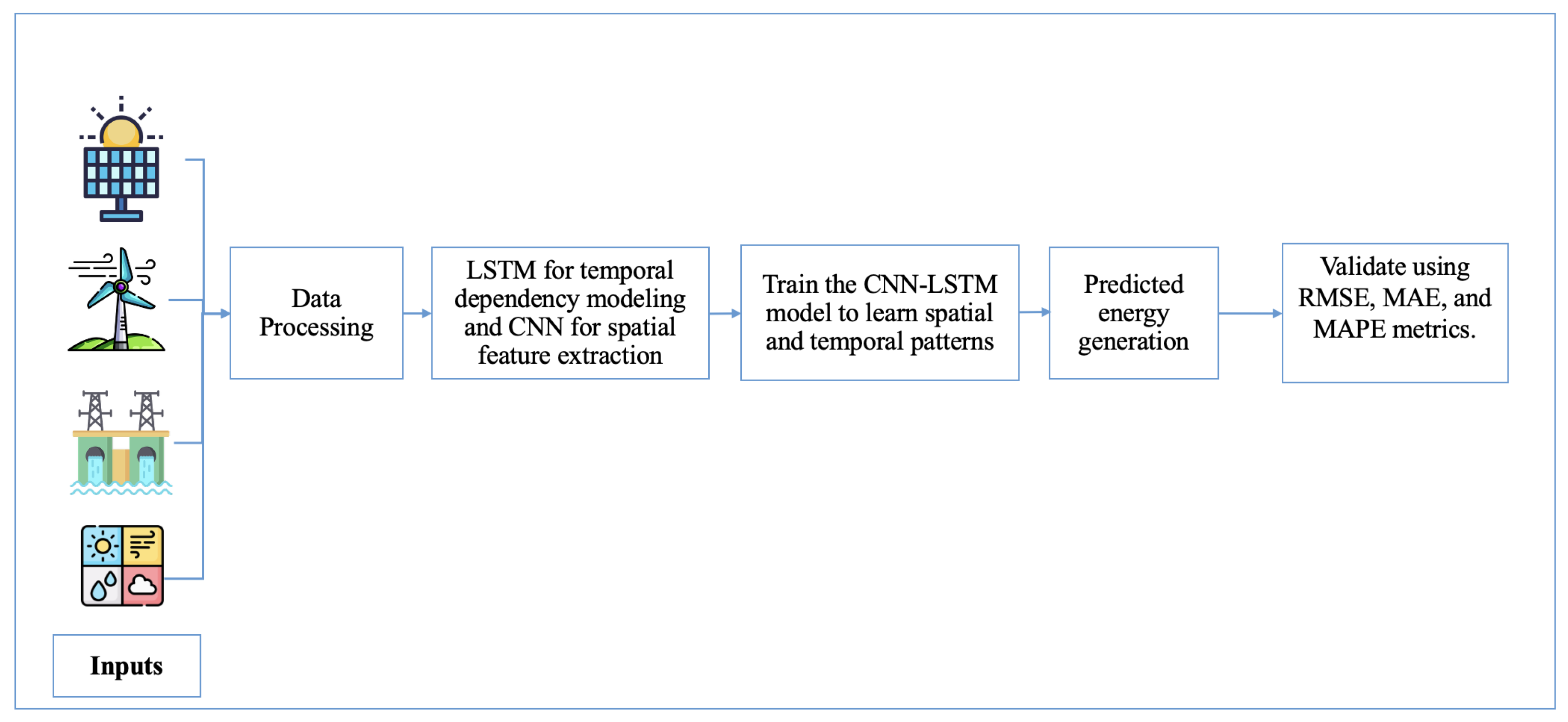
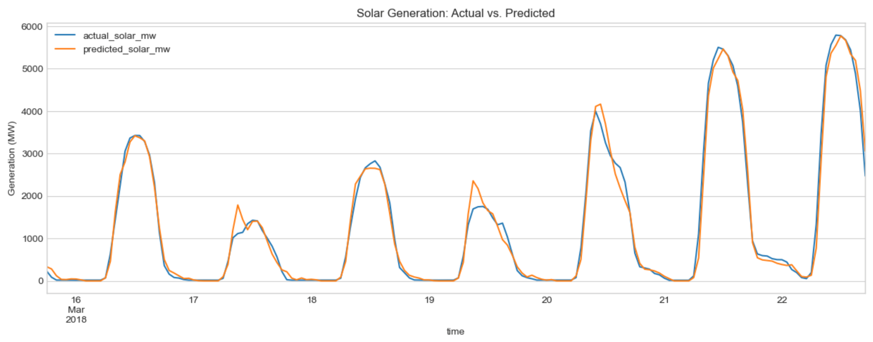
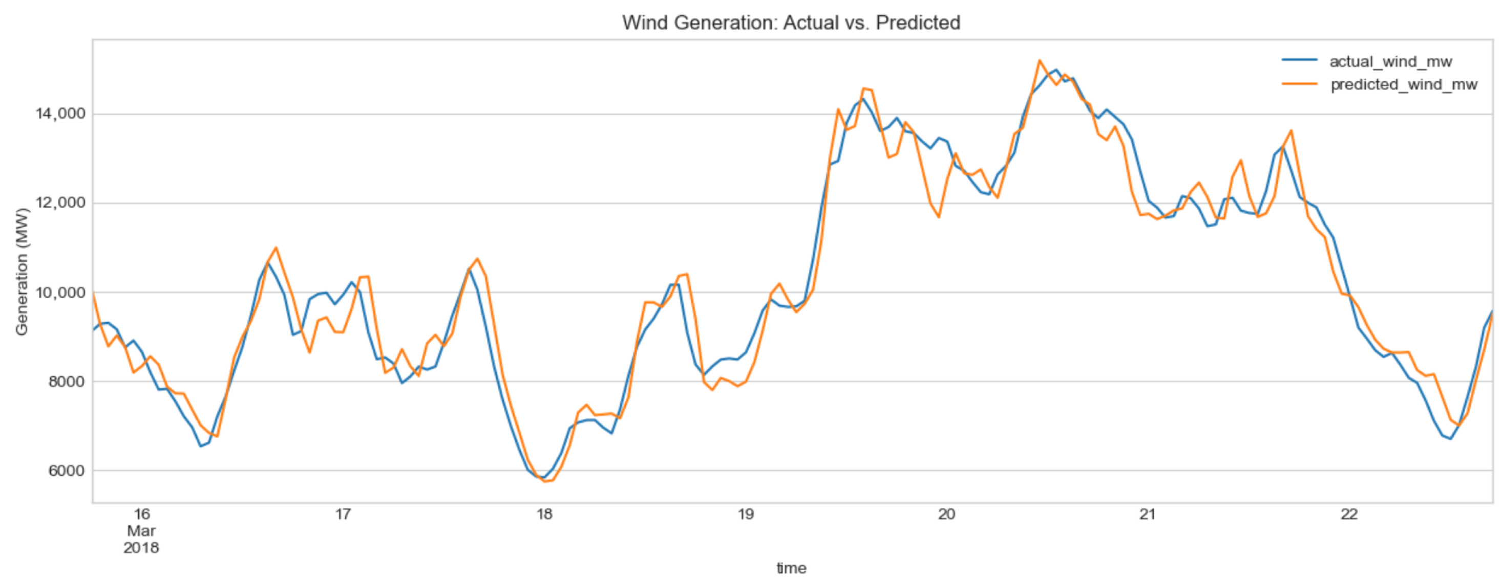
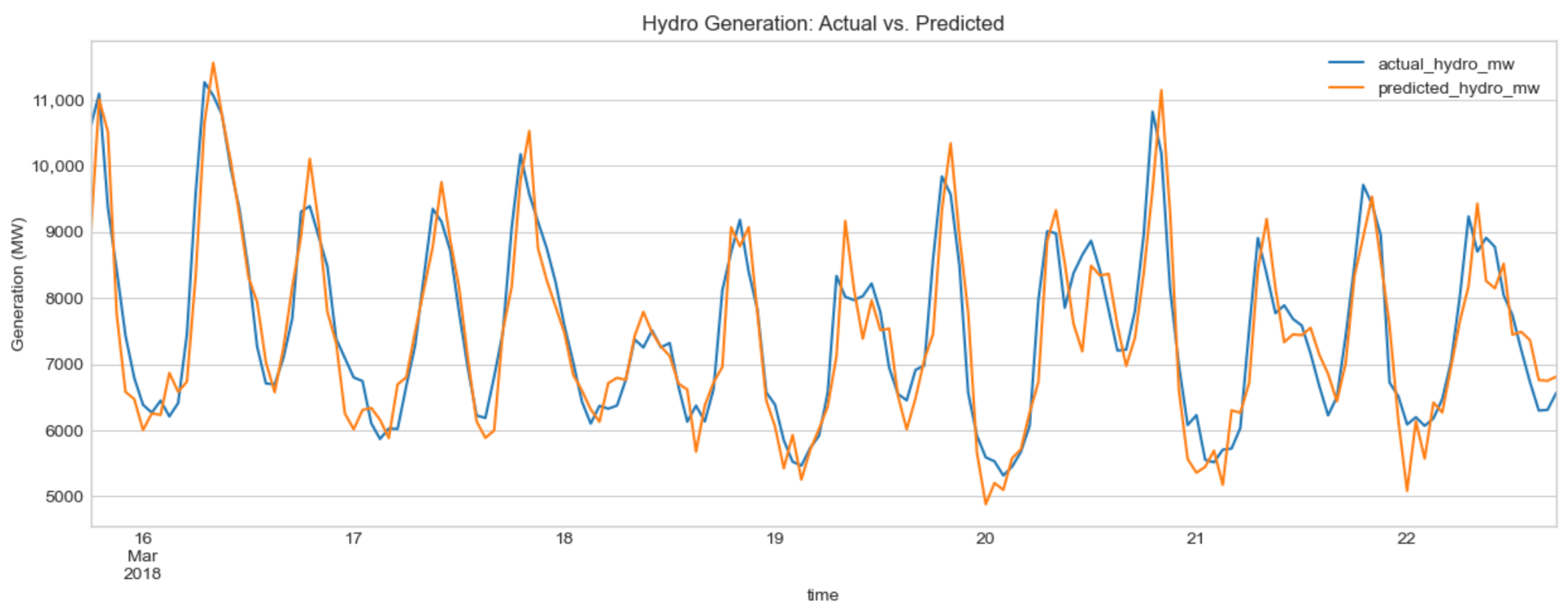
The first component illustrated in Figure 3 of the proposed framework focuses on forecasting renewable energy generation using a hybrid deep learning model that combines Convolutional Neural Networks (CNN) and Long Short-Term Memory (LSTM) units. The model was designed to capture both spatial correlations in meteorological variables and temporal dependencies in historical energy generation patterns. The input data consist of hourly records of renewable generation (solar, wind, and hydro) and corresponding weather features, including temperature, humidity, wind speed, and solar irradiance. The data are arranged as multivariate time-series windows, where each input sequence of length t (e.g., 24 h) is used to predict the next hour of generation. This 24 h window was specifically chosen to enable the model to learn from the full daily cycle of meteorological and behavioral patterns.

The model’s ability to learn from both spatial and temporal patterns is achieved through its hybrid architecture and the specific structure of its input data. The input consists of multivariate time-series windows where, at each time step, the feature vector contains simultaneous weather readings from all five geographically diverse cities. The CNN component operates on this structure to capture spatial relationships. While a one-dimensional (1D) convolution slides along the temporal axis, its filters process the full feature vector at each step. This enables the model to learn complex cross-locational correlations, such as the relationship between wind speeds in northern cities and solar irradiance in southern cities. The feature maps extracted by the CNN thus represent higher-level abstractions of the system’s spatial state. These feature maps are then passed to the stacked LSTM layers, which are specifically designed to model the long-range sequential dependencies and temporal trends within this spatially informed data, completing the spatio-temporal analysis.

A fully connected dense layer produces the final output values for each renewable source. Model training was performed using the Adam optimizer with Mean Absolute Error (MAE) as the loss function. Early stopping was applied with a patience of 10 epochs, meaning the training stopped if no improvement in validation loss occurred over 10 consecutive epochs. Dropout regularization was applied to both CNN and LSTM layers with a rate of 0.2 to prevent overfitting. The network was trained separately for each renewable type (solar, wind, and hydro), using the training and validation sets described in Section 3.2. The predicted outputs from this component provide hour-ahead renewable generation estimates that serve as inputs to the PSO module.

Table 3. CNN–LSTM architecture and training hyperparameters.

Parameter	Description/Value
Input shape	24 h time window, multivariate (weather + generation)
Convolutional layers	1D CNN, 64 filters, kernel size = 3, ReLU activation
Pooling layer	MaxPooling1D (pool size = 2)
LSTM layers	Two stacked LSTM layers, 64 and 32 units, dropout = 0.2
Dense layer	Fully connected, linear activation (output = generation forecast)
Loss function	Mean Absolute Error (MAE)
Optimizer	Adam, learning rate = 0.001
Training epochs	100 (with early stopping on validation loss, patience = 10)
Batch size	64
Dropout rate	0.2 (regularization for CNN and LSTM layers)
Validation split	0.2 (for training/validation split)
Output	Hourly renewable generation forecast (solar, wind, hydro) in MW

provides a detailed summary of the CNN–LSTM architecture, including input shape, convolutional and LSTM layers, loss function, optimizer, and other key hyperparameters used for model training.

3.6.2. Component 2: GBM for Energy Demand Forecasting

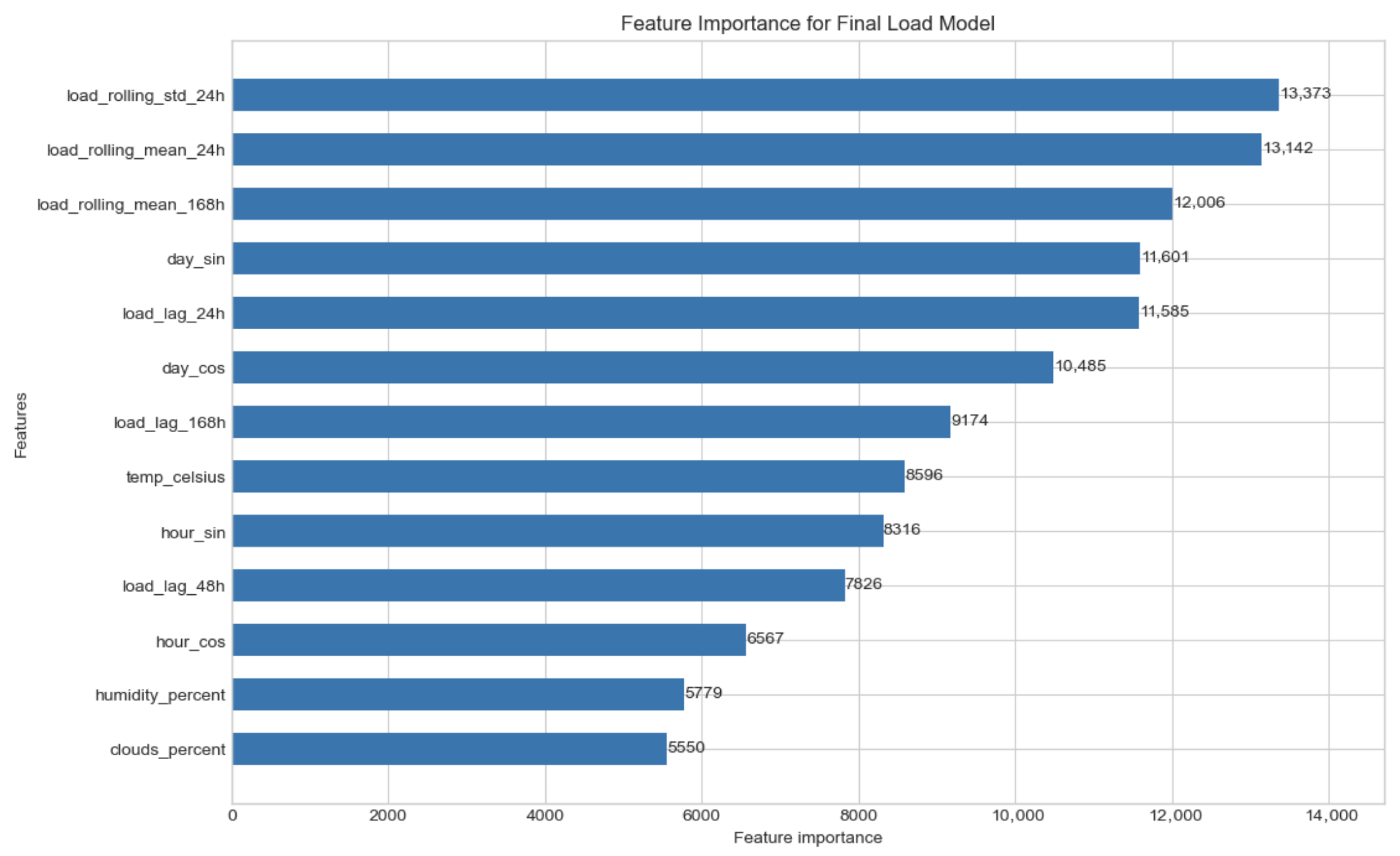
The second component presented in Figure 4 of the framework focuses on forecasting energy demand using Gradient Boosting Machines (GBMs), a tree-based ensemble learning algorithm known for its high predictive accuracy and interpretability. GBM was selected for this task due to its ability to model complex nonlinear relationships and handle heterogeneous input features efficiently, making it well-suited for energy consumption data influenced by both temporal and meteorological factors. The input features include historical electricity demand, temperature, humidity, wind speed, and time-based variables such as hour of day, day of week, and month. These were derived from the same preprocessed dataset described in Section 3.2. To capture short-term consumption dynamics, lag features and rolling averages of past demand were also incorporated. The model learns by sequentially constructing an ensemble of regression trees, where each new tree corrects the residual errors of the previous ensemble, gradually minimizing prediction loss.

To ensure a robust validation that simulates a real-world forecasting scenario and prevents any form of data leakage, the dataset was divided into training and testing sets using a single, strict chronological cutoff point. All data prior to the cutoff was used for training, and all subsequent data was used for testing. Hyperparameters such as learning rate, maximum tree depth, and the number of estimators were tuned using a grid search methodology applied only to the training data. The final model was then trained on the complete training set using the optimal hyperparameters and evaluated on the held-out test set.

Table 4. GBM model hyperparameters and training settings.

Parameter	Description/Value
Algorithm	Gradient Boosting Regressor (GBM)
Input features	Historical demand, weather variables, temporal encodings, lag features
Loss function	Mean Absolute Error (MAE)
Learning rate	0.05 (Final)
Max depth	6 (Final)
Number of estimators	400 (Final)
Subsample rate	0.8 (fraction of data used for each tree)
Cross-validation	Chronological train-test split
Hyperparameter tuning	Grid search to optimize MAE on a validation set
Output	Hourly energy demand forecast (MW)

provides a detailed summary of the key hyperparameters used in the Gradient Boosting Machine (GBM) model, including the loss function, learning rate, number of estimators, subsample rate, and hyperparameter tuning strategy. The tuning of these parameters was performed using a grid search approach to optimize the model’s performance. The GBM model predicts the hourly energy demand based on historical data, weather variables, and temporal features.

3.6.3. Component 3: Particle Swarm Optimization (PSO) for Energy Allocation

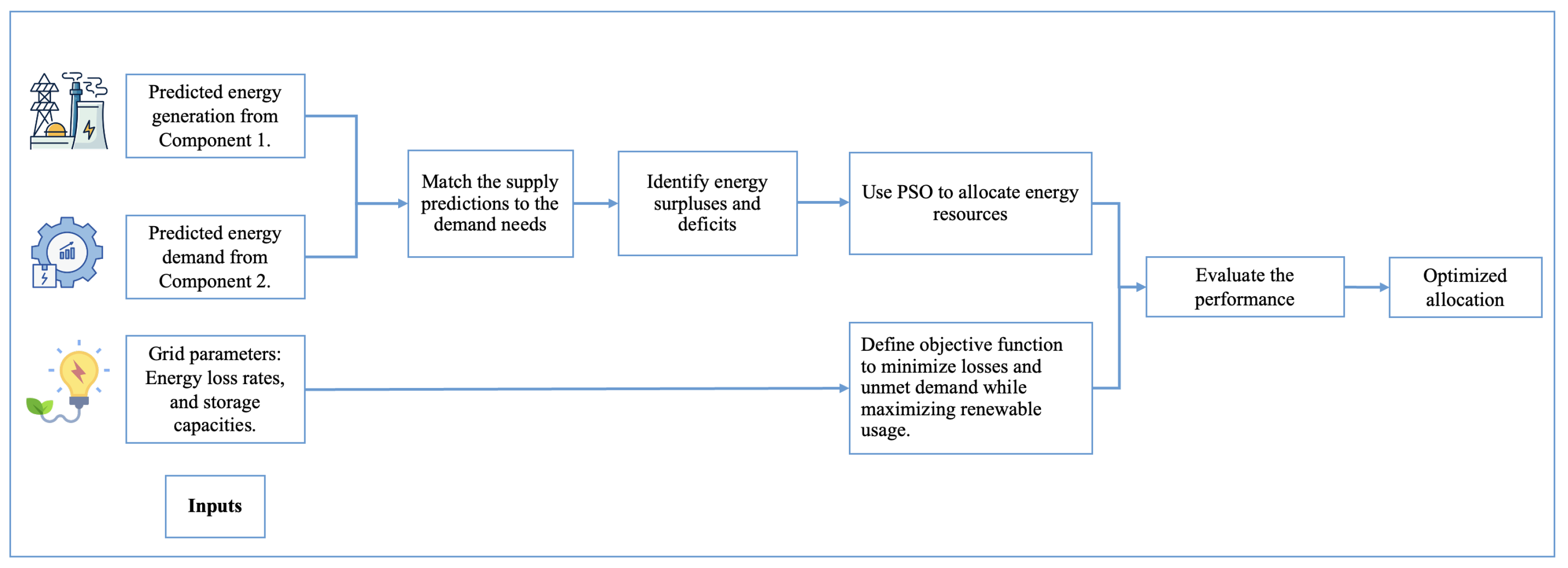
The third component shown in Figure 5 focuses on optimizing the energy allocation process using Particle Swarm Optimization (PSO), a population-based metaheuristic inspired by the collective behavior of birds and fish. PSO is applied here to efficiently allocate energy resources between renewable and conventional sources while balancing supply and demand. As a metaheuristic approach, PSO was selected for its effectiveness in navigating complex, nonlinear optimization problems, such as those involving the stochastic nature of renewables, without requiring gradient information. This provides a flexible alternative to more rigid, traditional methods like Mixed-Integer Linear Programming (MILP). Each particle in the swarm represents a candidate allocation vector $x=[x_1,x_2,x_3,x_4]$, where $x_1,x_2,x_3,x_4$ correspond to the energy shares allocated to solar, wind, hydro, and conventional sources, respectively.

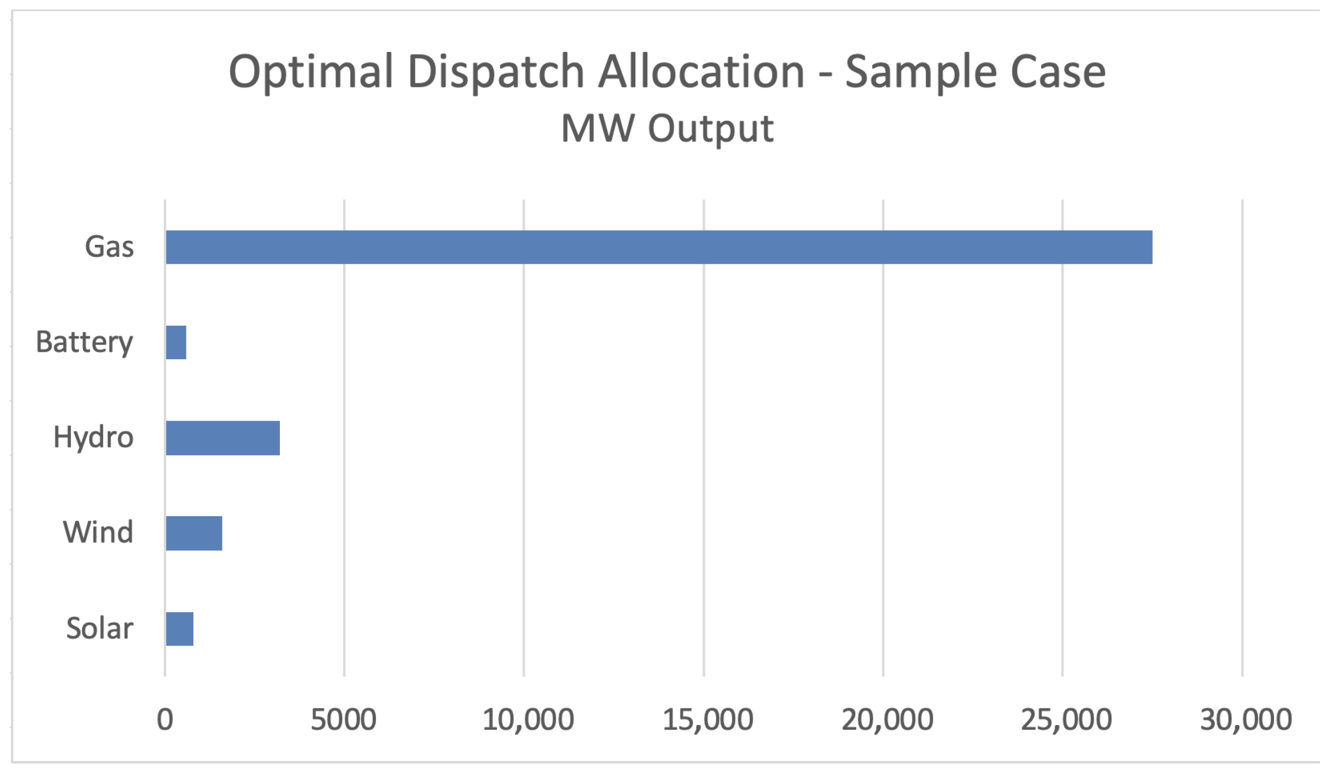
The primary objective of the PSO algorithm is to minimize the total operational cost of the system for each hour, subject to the fundamental constraint that the total energy supplied must equal the total energy demand (i.e., unmet demand must be zero). The cost function includes the direct costs of dispatchable generation (e.g., fuel for a gas turbine) and can also incorporate penalties for undesirable outcomes, such as the curtailment of available renewable energy. By searching for the allocation vector that minimizes this cost function while satisfying all constraints, the PSO finds a cost-effective and operationally feasible dispatch solution.

The optimization represents a simplified economic dispatch model. Key assumptions include linear cost functions for dispatchable generation, no cost for available renewable energy, and the absence of complex grid constraints such as ramp rates or transmission limits. The primary constraints are that total generation must meet total demand and that dispatch from each source cannot exceed its predefined capacity.

The PSO algorithm stops when the change in the global best fitness becomes negligible or after a predefined number of iterations (200). The final output of this component is an optimized energy allocation plan that balances generation and demand while reducing reliance on fossil fuels and improving grid efficiency. These results are subsequently used for further analysis and decision-making.

Table 5. PSO algorithm configuration and parameter settings.

Parameter	Description/Value
Algorithm	Particle Swarm Optimization (PSO)
Objective function	Minimize cost and unmet demand; maximize renewable utilization
Decision variables	Energy allocation shares (solar, wind, hydro, conventional)
Swarm size	50 particles
Inertia weight (w)	0.7
Cognitive coefficient ($c_1$)	1.5
Social coefficient ($c_2$)	1.5
Maximum iterations	200
Stopping criterion	Convergence of global best fitness
Output	Optimized hourly energy allocation

provides a summary of the key hyperparameters and configuration settings used for the Particle Swarm Optimization (PSO) algorithm. These parameters were tuned to optimize the allocation of energy resources, balancing cost reduction with maximizing renewable energy utilization. The PSO algorithm was configured with specific values for the inertia weight, cognitive and social coefficients, and the number of iterations to ensure effective exploration and exploitation of the solution space.

3.7. Model Evaluation and Performance Metrics

The framework’s performance was evaluated separately for forecasting (CNN-LSTM and GBM) and optimization (PSO). Forecasting performance was measured using Mean Absolute Error (MAE) [29], Root Mean Square Error (RMSE) [30], and the Coefficient of Determination ($R^2$) [31]. For the optimization component, the effectiveness of PSO was evaluated using Cost Reduction (CR), Renewable Utilization (RU), and Grid Efficiency (GE).

For the forecasting models, the performance was calculated as follows:

$$\mathrm{MAE}={\displaystyle \frac{1}{N}}\sum _{i=1}^N|y_i-{\widehat{y}}_i|,$$

(1)

$$\mathrm{RMSE}=\sqrt{{\displaystyle \frac{1}{N}}\sum _{i=1}^N{(y_i-{\widehat{y}}_i)}^2},$$

(2)

$$R^2=1-{\displaystyle \frac{{\sum }_{i=1}^N{(y_i-{\widehat{y}}_i)}^2}{{\sum }_{i=1}^N{(y_i-\overline{y})}^2}},$$

(3)

Additionally, Mean Absolute Percentage Error (MAPE) was calculated to provide a scale-independent measure of forecast accuracy.

$$\mathrm{MAPE}={\displaystyle \frac{100\%}{n}}\sum _{i=1}^n\left|{\displaystyle \frac{y_i-{\widehat{y}}_i}{y_i}}\right|$$

(4)

where $y_i$ and ${\widehat{y}}_i$ denote the actual and predicted values, $\overline{y}$ is the mean of actual values, and N is the number of observations. Lower MAE and RMSE values indicate higher accuracy, while an $R^2$ value closer to 1 indicates a stronger fit of the model to the data.

For the optimization component (PSO), the performance was quantified using the following three key metrics:

$$\mathrm{CR}={\displaystyle \frac{C_{\mathrm{base}}-C_{\mathrm{PSO}}}{C_{\mathrm{base}}}}\times 100,$$

(5)

where $C_{\mathrm{base}}$ is the baseline operational cost and $C_{\mathrm{PSO}}$ is the operational cost after PSO.

$$\mathrm{RU}={\displaystyle \frac{E_{\mathrm{renewable}}}{E_{\mathrm{total}}}}\times 100,$$

(6)

where $E_{\mathrm{renewable}}$ is the energy generated from renewable sources, and $E_{\mathrm{total}}$ is the total energy generation.

$$\mathrm{GE}=\left(1-{\displaystyle \frac{P_{\mathrm{unmet}}}{P_{\mathrm{demand}}}}\right)\times 100,$$

(7)

where $P_{\mathrm{unmet}}$ is the unmet demand and $P_{\mathrm{demand}}$ is the total required demand.

These metrics jointly quantify the predictive accuracy of the forecasting models and the operational effectiveness of the PSO in balancing supply and demand.

3.8. Tools and Technologies Used

The implementation of the proposed spatio-temporal predictive framework required an integrated environment of programming languages, scientific libraries, and computational resources to ensure accurate modeling, efficient training, and reproducible experimentation. All stages of the workflow—from data preprocessing and feature engineering to model training, optimization, and visualization—were implemented using open-source Python-based frameworks. Python was selected due to its strong ecosystem of libraries supporting deep learning, time-series forecasting, and optimization. The key software and hardware tools employed are summarized in

Table 6. Software and hardware tools used in the implementation.

Category	Tool and Version
OS/Hardware	Apple MacBook Air (M1, 2020), 8 GB RAM
Language	Python 3.10
Notebooks	Jupyter Notebook
Visualization	Matplotlib 3.9, Seaborn 0.13.2
Data handling	Pandas 2.2.3, NumPy 1.26.4
Machine learning	scikit-learn 1.6.1 (GBM)
Deep learning	TensorFlow 2.18.0 (CNN–LSTM)
Optimization	PySwarms 1.3.0 (PSO)

.

4. Results

4.1. Forecasting Performance

The proposed hybrid framework was evaluated using the test partition of the Spain 2015–2018 dataset. The CNN-LSTM model was trained separately for each renewable source (solar, wind, and hydro), while the GBM model predicted total energy demand.

Table 7. Forecasting performance of CNN-LSTM and GBM models on the Spanish dataset.

Model	MAE (MW)	RMSE (MW)	R2 Score	MAPE (%)
Solar Generation (CNN-LSTM)	11.42	15.87	0.9903	14.85
Wind Generation (CNN-LSTM)	23.11	29.45	0.9646	5.12
Hydro Generation (CNN-LSTM)	31.76	37.29	0.9302	3.98
Total Energy Demand (GBM)	18.64	23.73	0.9156	0.45

summarizes the forecasting accuracy obtained using the MAE, RMSE, and $R^2$ metrics. The results confirm that the spatio-temporal modeling approach effectively captures both sensor variability and temporal dependencies.

4.2. Feature Importance Analysis

This Figure 6 shows which factors are most important in predicting energy demand. It highlights the role of past load patterns (like the 24 h and 168 h averages) and time-based features (hour of the day and day of the week). Environmental factors, such as temperature, humidity, and cloud cover, also play a key role in the predictions, helping to improve the model’s accuracy. The high importance of the 24 h (load_lag_24h) and 168 h (load_rolling_mean_168h) features is particularly noteworthy, as it empirically confirms the strong influence of daily and weekly cyclical patterns (e.g., workdays vs. weekends) on energy demand.

4.3. Visuals Comparison of Actual and Predicted Values

Figure 7, Figure 8, Figure 9 and Figure 10 presents a comparison of actual versus predicted (solar, wind, and hydro) power renewable generation and demand. The close alignment between both series confirms the model’s capacity to track daily fluctuations and capture both peak and off-peak variations.

4.4. Energy Gap Analysis

This analysis centers on the concept of “Net Load,” which is defined as the total forecasted energy demand minus the total forecasted renewable generation (Net Load = Demand − Renewables). Figure 11 illustrates an energy gap analysis, comparing the predicted and actual net load over a two-week period. The red line represents the forecasted energy demand, while the dotted black line shows the actual demand. The green shaded area indicates periods of energy surplus, where generation exceeds demand, and the red shaded area highlights energy deficits, where additional generation is needed. This analysis is crucial for evaluating the accuracy of energy demand predictions, identifying discrepancies, and improving forecasting models. The benefits include optimizing energy generation, reducing waste, enhancing storage strategies, and ensuring a reliable power supply in smart cities by better aligning predictions with real-time demands.

4.5. Optimization Outcomes

To quantify the benefits of the PSO-based optimization, the proposed framework’s performance was compared against a baseline, non-optimized scenario. In this baseline, it was assumed that all available renewable energy would be utilized first, and any remaining Net Load (the gap between demand and renewable generation) would be met entirely by the most expensive dispatchable asset, the gas turbine, without the use of battery storage. The Particle Swarm Optimization (PSO) algorithm was then applied using the predicted renewable generation and demand as inputs to minimize operational costs while maximizing renewable utilization. The optimization results, summarized in

Table 8. Optimization outcomes comparing baseline and PSO-based energy allocation.

Scenario	Cost Reduction (%)	Renewable Utilization (%)	Grid Efficiency (%)
Baseline (no PSO)	0	42	85
Proposed (PSO)	18.2	54	97

, show significant improvements compared to the baseline allocation.

The application of PSO-based optimization led to an 18.2% reduction in operational costs and a 12% improvement in renewable utilization compared to the baseline scenario. Additionally, grid efficiency improved significantly, rising from 85% in the baseline scenario to 97% with PSO. These results demonstrate the effectiveness of the PSO framework in supporting energy management decisions, ensuring higher renewable penetration and improved grid performance. To illustrate the practical application of this allocation strategy, Figure 12 displays a sample dispatch profile during a high-demand hour.

5. Discussion

The experimental results from the Spanish dataset demonstrate that the proposed spatio-temporal framework can effectively forecast energy generation and demand and subsequently optimize resource allocation. The integrated CNN-LSTM-GBM-PSO approach establishes a continuous link from prediction to operational decision-making, with the high accuracy scores validating the core architecture. To more rigorously assess the robustness and broader applicability of this framework, a comprehensive generalization study was conducted using a dataset from a different national grid.

5.1. Framework Generalization on the German Dataset

To explicitly test the generalizability of the framework, the entire methodology was applied to a separate, publicly available dataset for the German energy market covering the period 2019–2022 [32]. Following our spatio-temporal approach, data was used from five geographically diverse federal states chosen to represent Germany’s varied energy landscape: Berlin (BE), Brandenburg (BB), Bavaria (BY), North Rhine-Westphalia (NRW), and Schleswig-Holstein (SH). The corresponding hourly meteorological data for these states was acquired from the NASA POWER database [33]. This provided a robust test case, as Germany has a different climate profile, a higher wind penetration, and a more complex, managed hydro system compared to Spain.

Despite these differences, the framework demonstrated excellent and consistent performance when trained on the German data, as summarized in

Table 9. Summary of Forecasting Performance on the German Dataset (2019–2022).

Model	MAE (MW)	RMSE (MW)	R2 Score
Solar Generation (CNN-LSTM)	486.11	493.69	0.9930
Wind Generation (CNN-LSTM)	359.57	363.96	0.9794
Hydro Generation (CNN-LSTM)	210.57	212.85	0.7700
Total Energy Demand (GBM)	967.65	967.65	0.9481

. The spatio-temporal CNN-LSTM model achieved outstanding accuracy for solar (R² = 0.993) and wind (R² = 0.980) forecasting, results that are directly comparable to those from the Spanish study. The GBM model for demand prediction also yielded a high R² of 0.948, even surpassing the performance on the Spanish data. This strong performance across a different geographical and meteorological landscape provides powerful empirical evidence that the proposed feature engineering strategies, model architectures, and integrated workflow are robust and can be effectively generalized to different national energy systems.

5.2. Limitations and Future Work

Despite the promising results, this study has some limitations that provide clear directions for future research. First, a primary limitation is the absence of a direct performance comparison against established baseline models. While the framework demonstrates high accuracy, a comprehensive benchmarking against classical methods (e.g., ARIMA, persistence models) and alternative deep learning architectures (e.g., standard LSTM or Transformer networks) is a critical next step. Such an analysis would more formally quantify the performance gains of the proposed hybrid approach.

Second, the disparity in performance for the hydro model between the Spanish (R² = 0.93) and German (R² = 0.77) case studies highlights a limitation of the framework’s primary reliance on meteorological data. This finding suggests that German hydropower is more significantly influenced by non-weather-related, anthropogenic factors, such as complex river management for shipping navigation or grid balancing operations with pumped storage. This demonstrates that while the framework is robust, its accuracy for certain targets is constrained by the scope of its input features. Future work could integrate economic data (e.g., electricity prices) or direct hydrological data (e.g., river flow rates) to improve forecasting in such complex, human-managed systems.

Third, the optimization module employs a simplified economic dispatch model. The current study does not include complex operational constraints such as network ramp rates or transmission limits. Future work should incorporate a more detailed grid model and would also benefit from sensitivity analyses on key cost and capacity parameters to assess the robustness of the dispatch solutions.

Finally, the current framework provides deterministic point forecasts. For operational grid management, quantifying forecast uncertainty is crucial. Future iterations should explore probabilistic forecasting methods, such as using quantile loss functions or Bayesian deep learning, to generate prediction intervals and provide a richer basis for risk-aware decision-making. Furthermore, the interpretability of the models could be deepened by applying techniques such as SHAP (SHapley Additive exPlanations) to the GBM or visualizing the learned convolutional filters to better understand the spatio-temporal patterns captured by the CNN-LSTM, yielding greater insights into the models’ behavior.

6. Conclusions

This study proposed and validated an integrated spatio-temporal artificial intelligence framework for renewable energy generation and demand forecasting in smart cities. The framework successfully combines a CNN–LSTM network for renewable generation forecasting, a GBM for interpretable energy demand prediction, and a PSO algorithm for energy allocation and cost minimization.

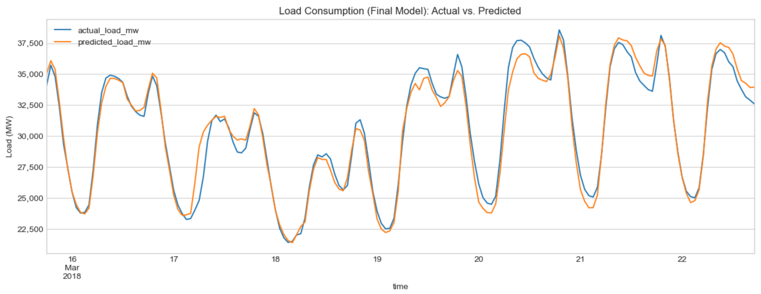
The framework’s primary validation on Spain’s national energy dataset (2015–2018) demonstrated its ability to effectively capture cross-locational weather correlations and temporal dynamics, achieving high forecasting accuracy with R² values of 99.03% for solar, 96.46% for wind, and 93.02% for hydro, while the demand model reached 91.56%. To rigorously test the framework’s generalizability—a key contribution of this revised work—the entire methodology was successfully applied to a German dataset, yielding similarly high performance (e.g., R² of 0.993 for solar and 0.948 for demand). This successful validation across two distinct national energy systems provides strong evidence that the proposed architecture is robust and adaptable.

Integrating PSO with these predictive components enhanced operational outcomes, reducing total costs by 18.2% in the Spanish case study. These results underscore the framework’s capacity to improve decision-making for grid scheduling, optimize resource allocation, and support sustainability goals in sensor-enabled urban environments. The primary contribution of this paper lies in integrating deep learning for prediction and metaheuristic optimization within a single, validated end-to-end architecture, creating a practical, data-driven system suitable for real-world energy management platforms. The proposed framework provides a foundation for the future development of autonomous smart-grid control systems. As discussed, future work will focus on benchmarking against state-of-the-art models, incorporating probabilistic forecasting to quantify uncertainty, and expanding the model with economic and hydrological data. These advancements will further enhance system resilience and enable more proactive energy management in emerging smart cities.