Study on the Economic Benefits of Gas–Wind–Solar Power Alliance Under Gas Peaking Mode
Abstract
1. Introduction
- (1)
- How can an optimization model capable of quantitatively evaluating the economic benefits of gas–wind–solar alliance power generation systems under natural gas peak shaving modes be constructed?
- (2)
- How can the overall benefits of gas–wind–solar alliances and the operational characteristics of natural gas power units be evaluated under typical wind and solar output scenarios?
- (3)
- How sensitive are the economic benefits and environmental impacts of gas–wind–solar alliances to changes in key parameters (such as gas prices, electricity prices, and carbon prices) under different market mechanisms and policy environments?
2. Problem Description and Symbol Definitions
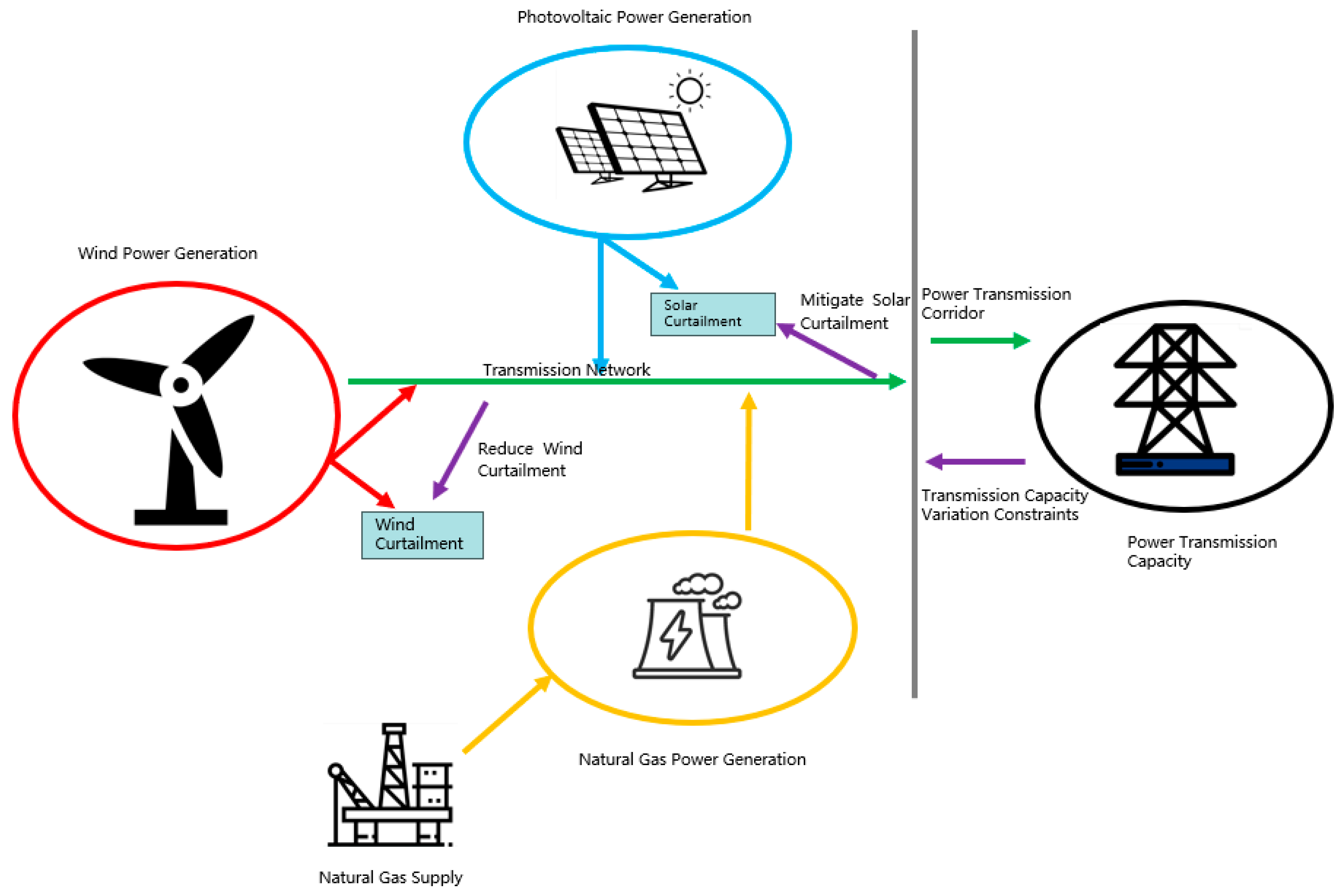
2.1. Problem Description
2.2. Nomenclature
2.2.1. Indicator Set
2.2.2. Symbol Definitions
3. Gas–Wind–Solar Hybrid Power Generation Model Construction and Solution
3.1. Model Construction
3.1.1. Objective Function
- (1)
- System Operating Income
- (2)
- Green Certificate Trading Revenue
- (3)
- System Operating Cost
- (4)
- Wind and Solar Curtailment Penalty Cost
- (5)
- Gas-fired Carbon Emission Penalty Cost
3.1.2. Binding Conditions
- (1)
- Power Constraint of the Gas–Wind–Solar Hybrid Power Generation
- (2)
- Power Variation Constraint for Hybrid Power Generation
- (3)
- Rotational Reserve Capacity Constraint of the Gas–Wind–Solar Hybrid Power Generation System
- (4)
- Gas-fired unit output constraints
- (5)
- Minimum Start-up and Shut-down Time Constraints for Gas-fired Units
- (6)
- Wind Power Output Constraint
3.2. Model Solution Strategy
- (1)
- Objective Function Linearization
- (2)
- Linearization of Constraints
- (3)
- Model Solving
4. Results and Discussion
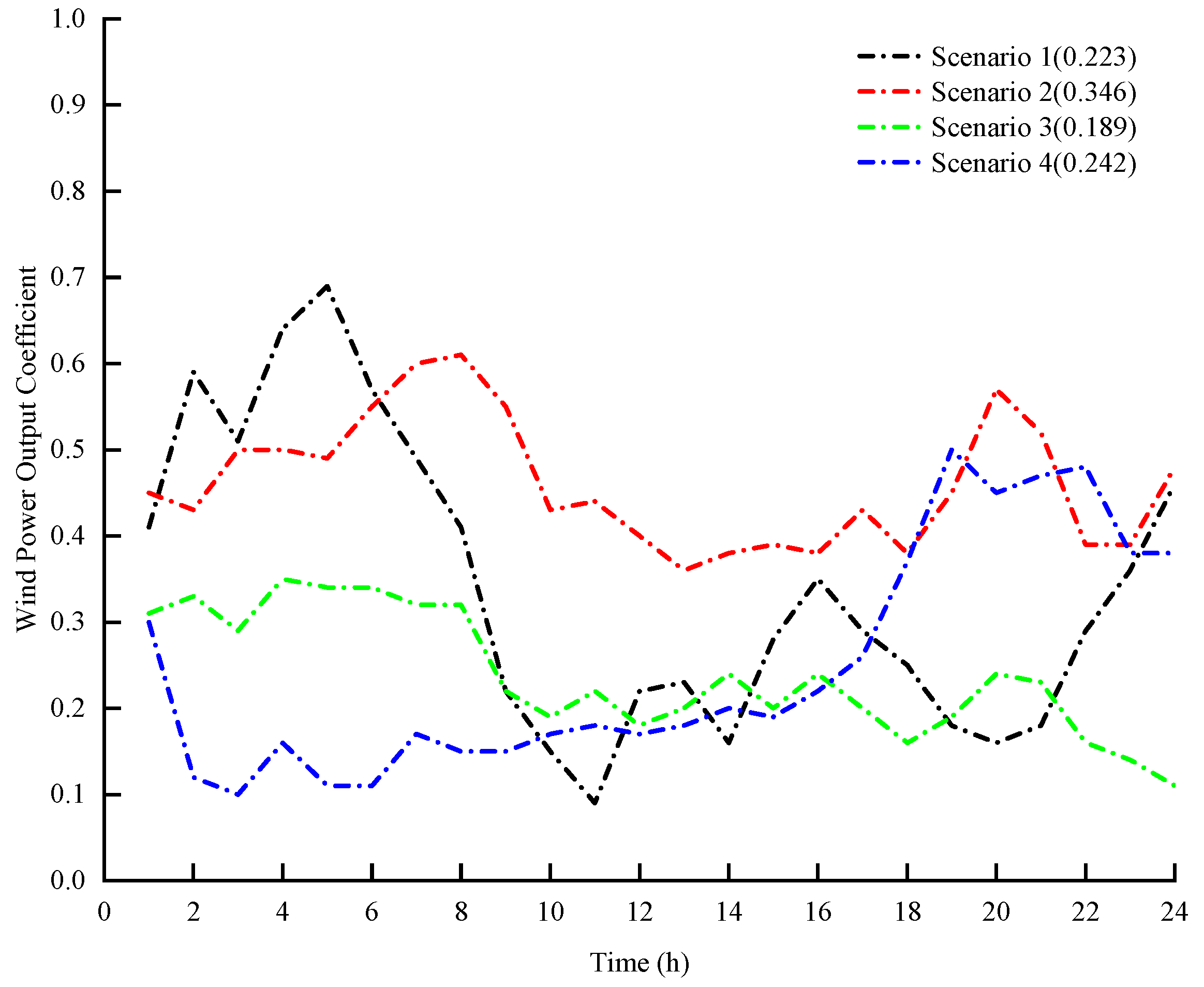
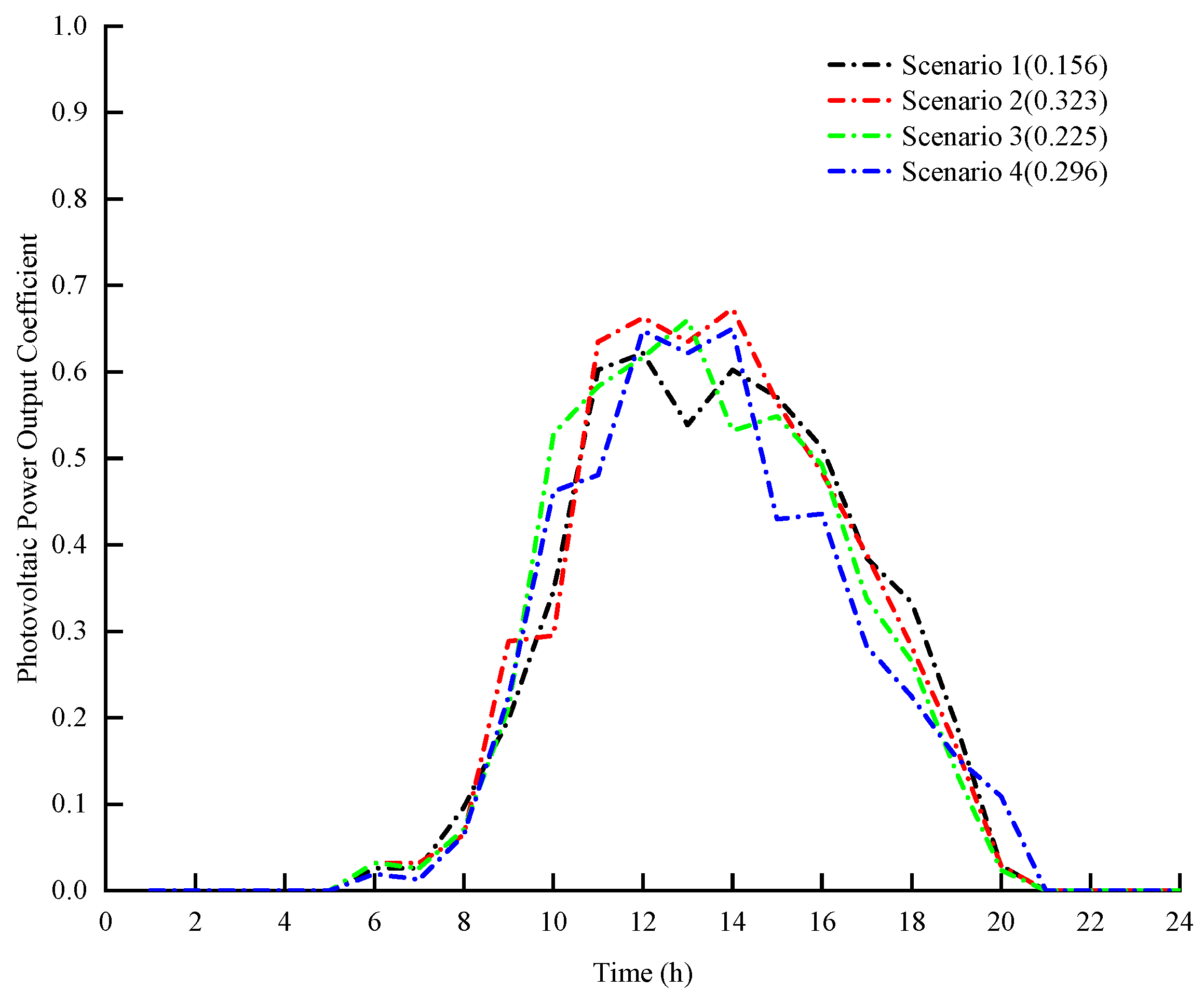
4.1. Basic Information
4.2. Simulation Results
- (1)
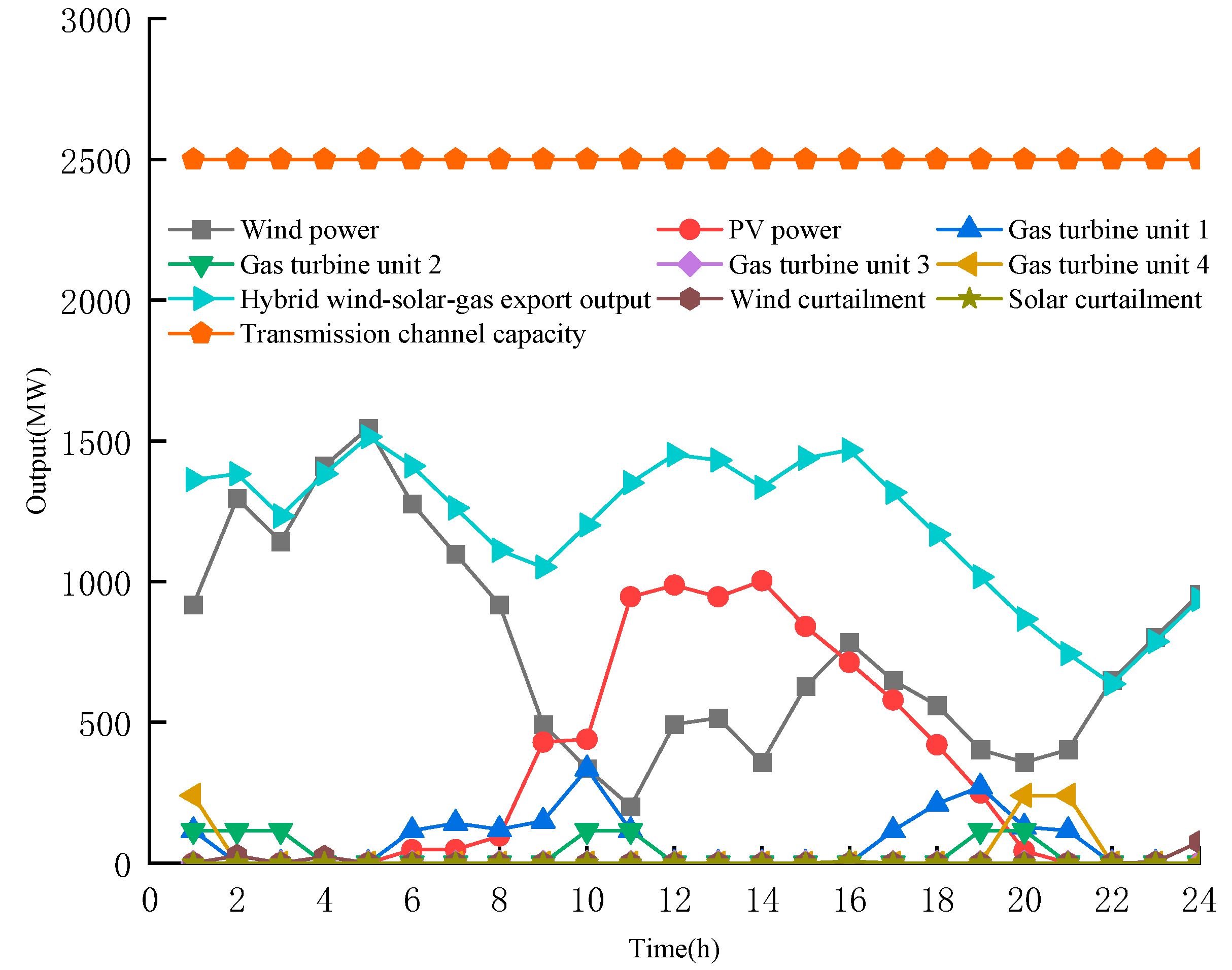
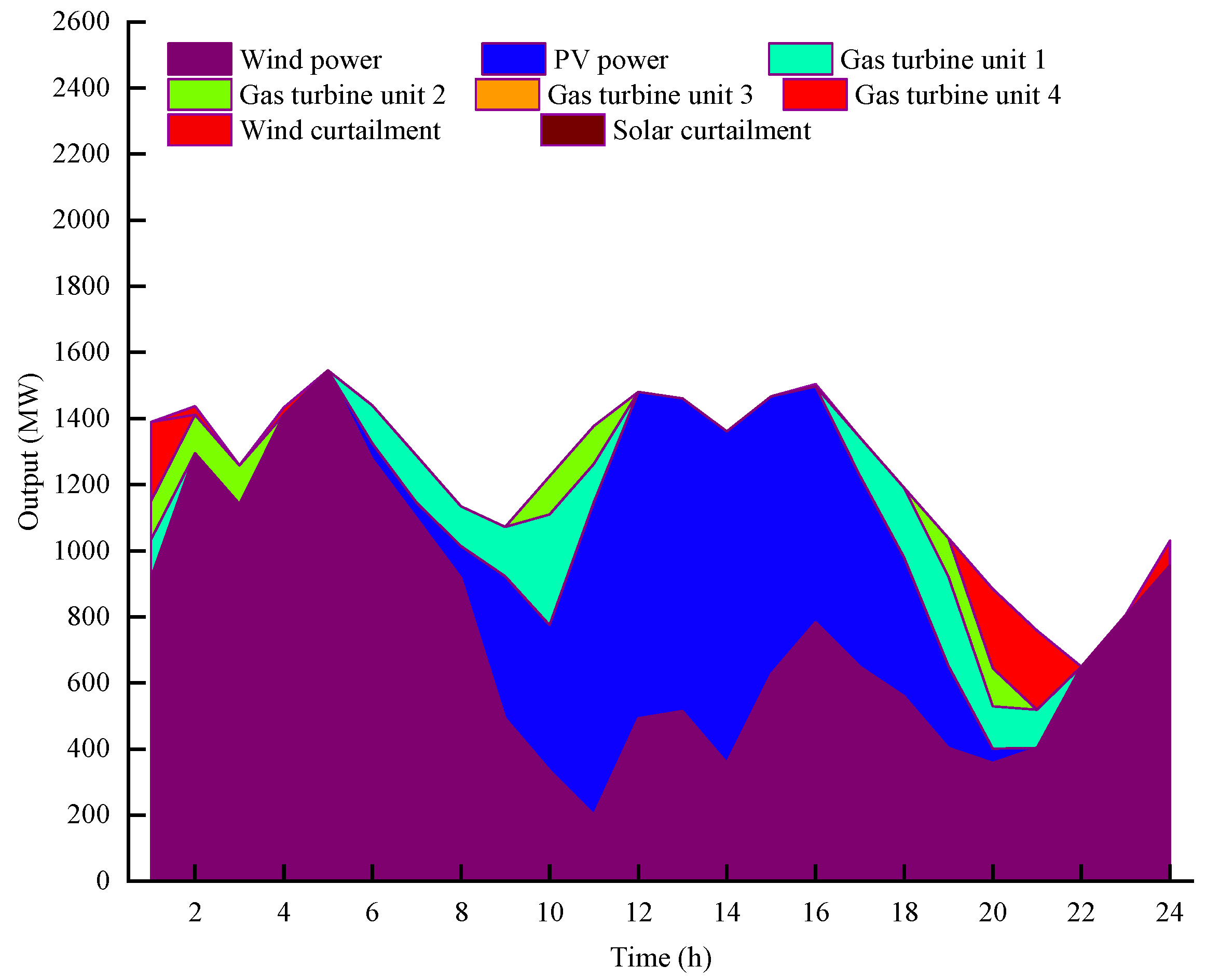
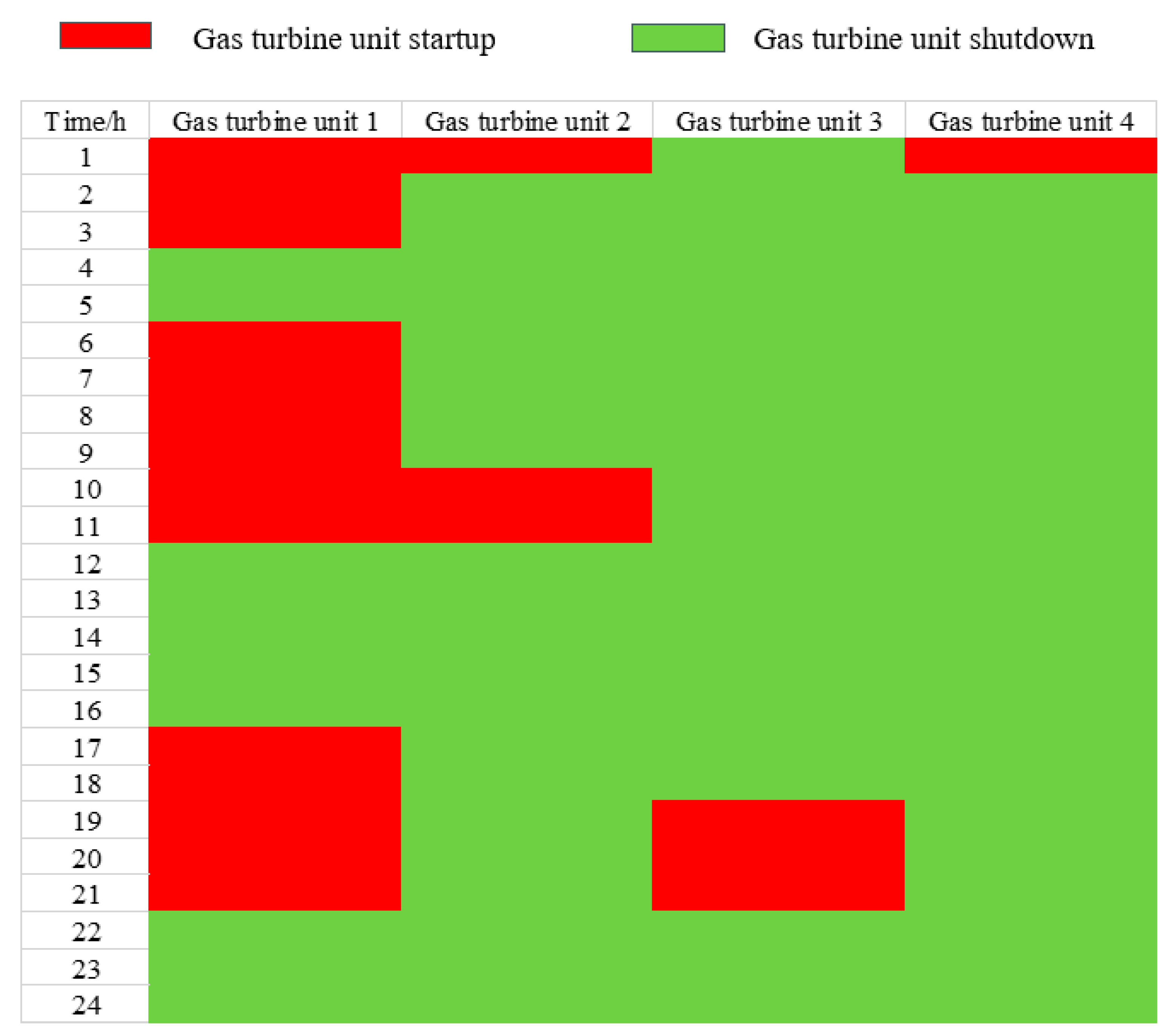
- Analysis of Typical Operation Scenarios
- (2)
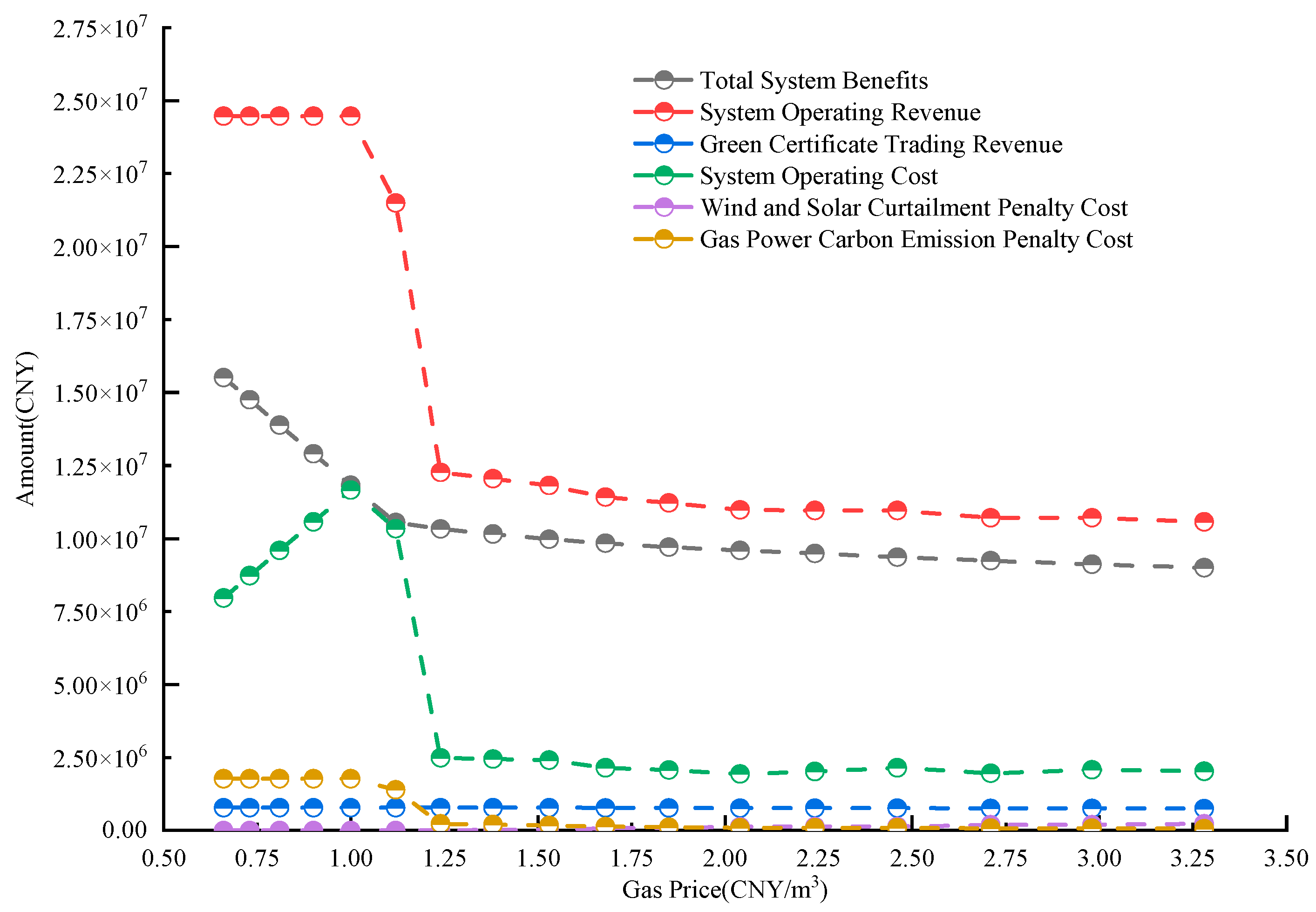
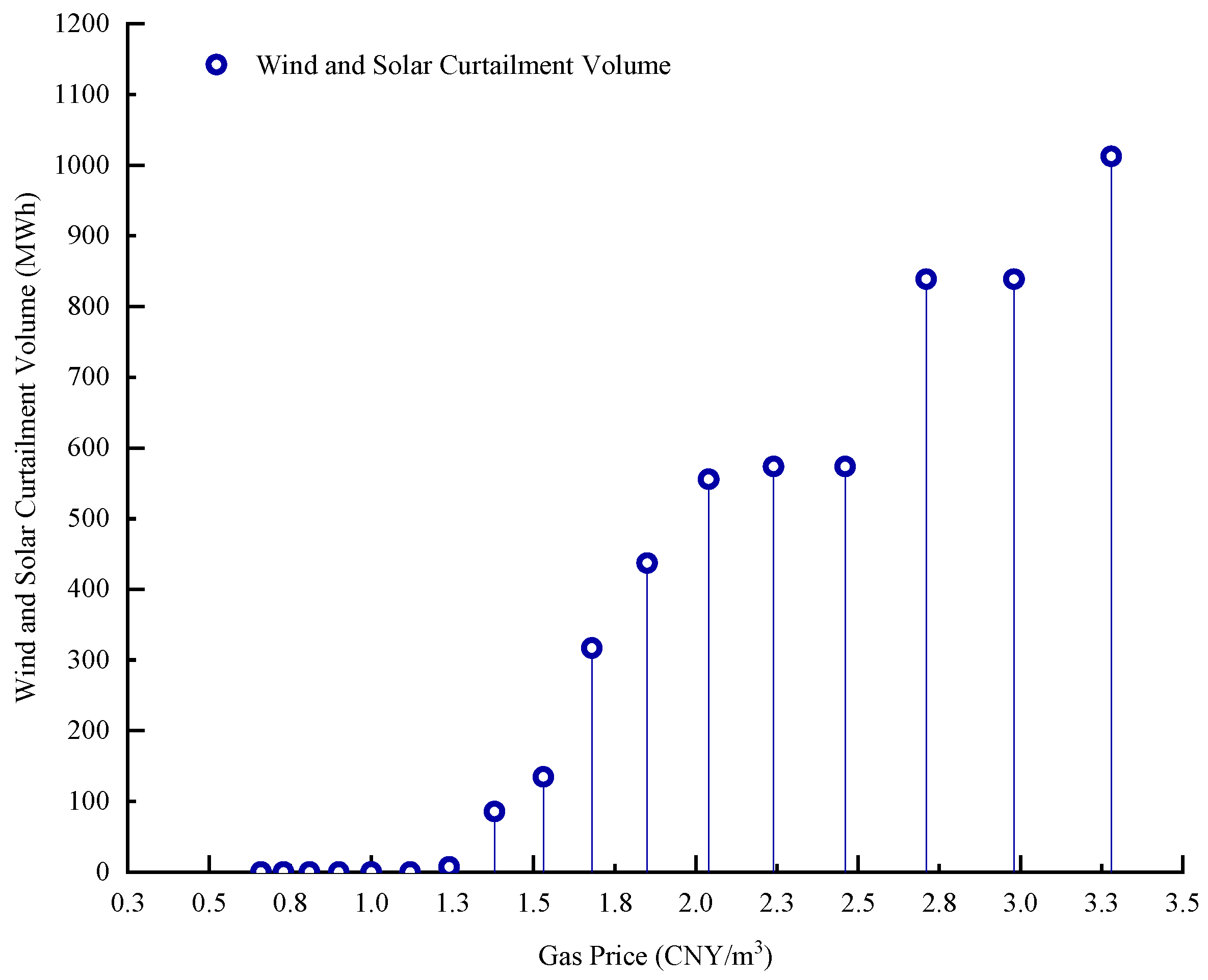
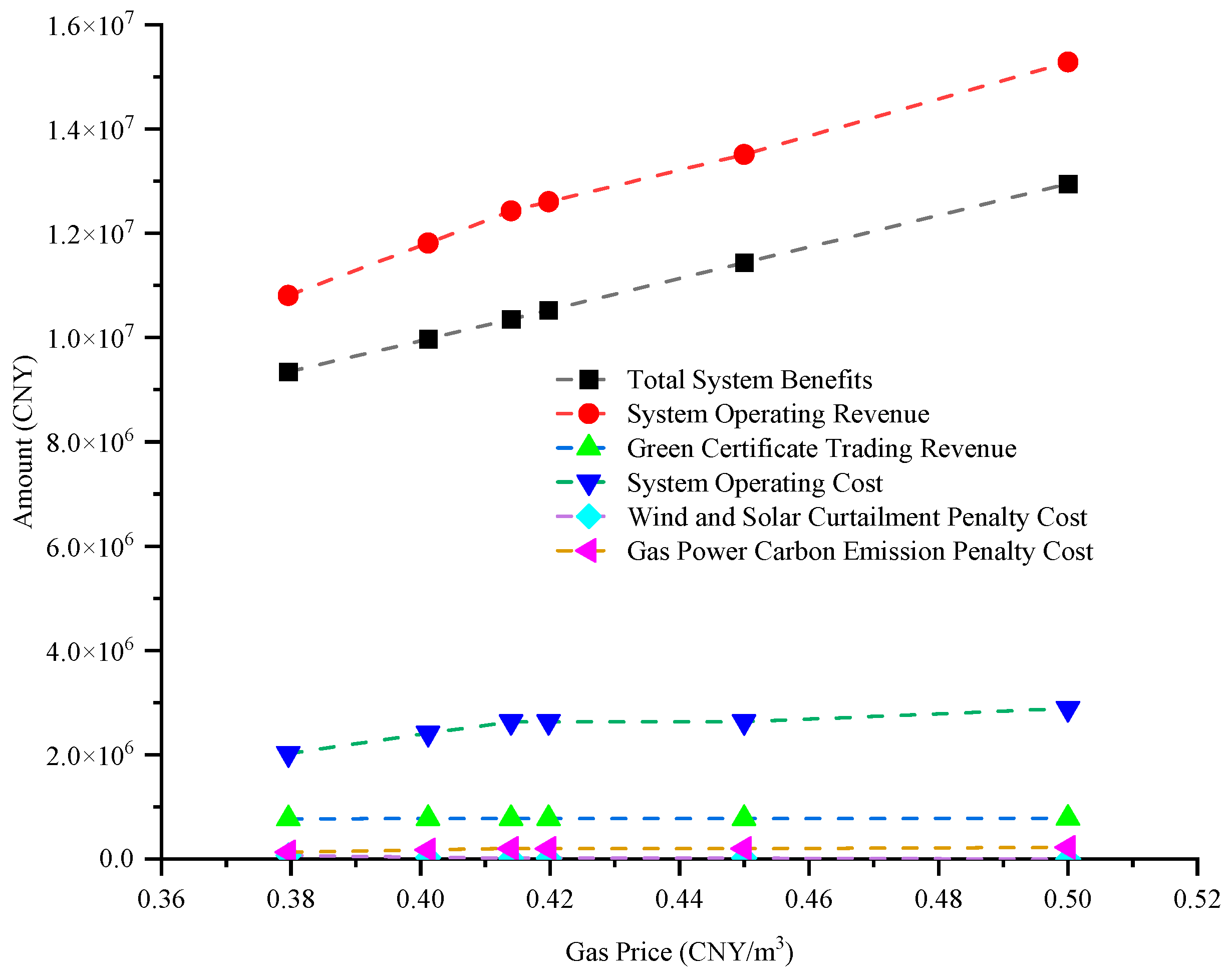
- Impact of Natural Gas Price on System Economic Indicators
- (3)
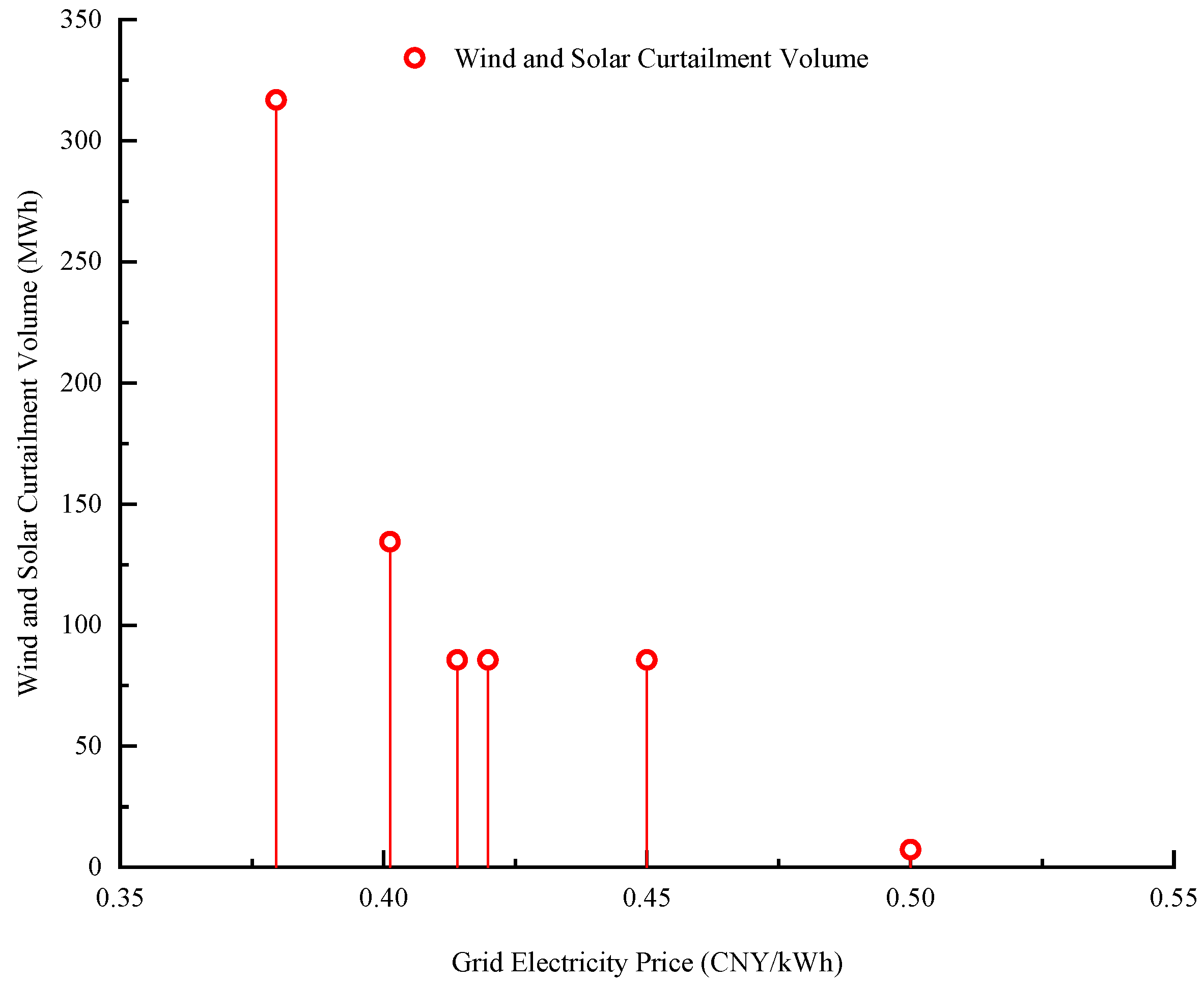
- Impact of Grid-connected Electricity Price on System Economic Indicators
- (4)
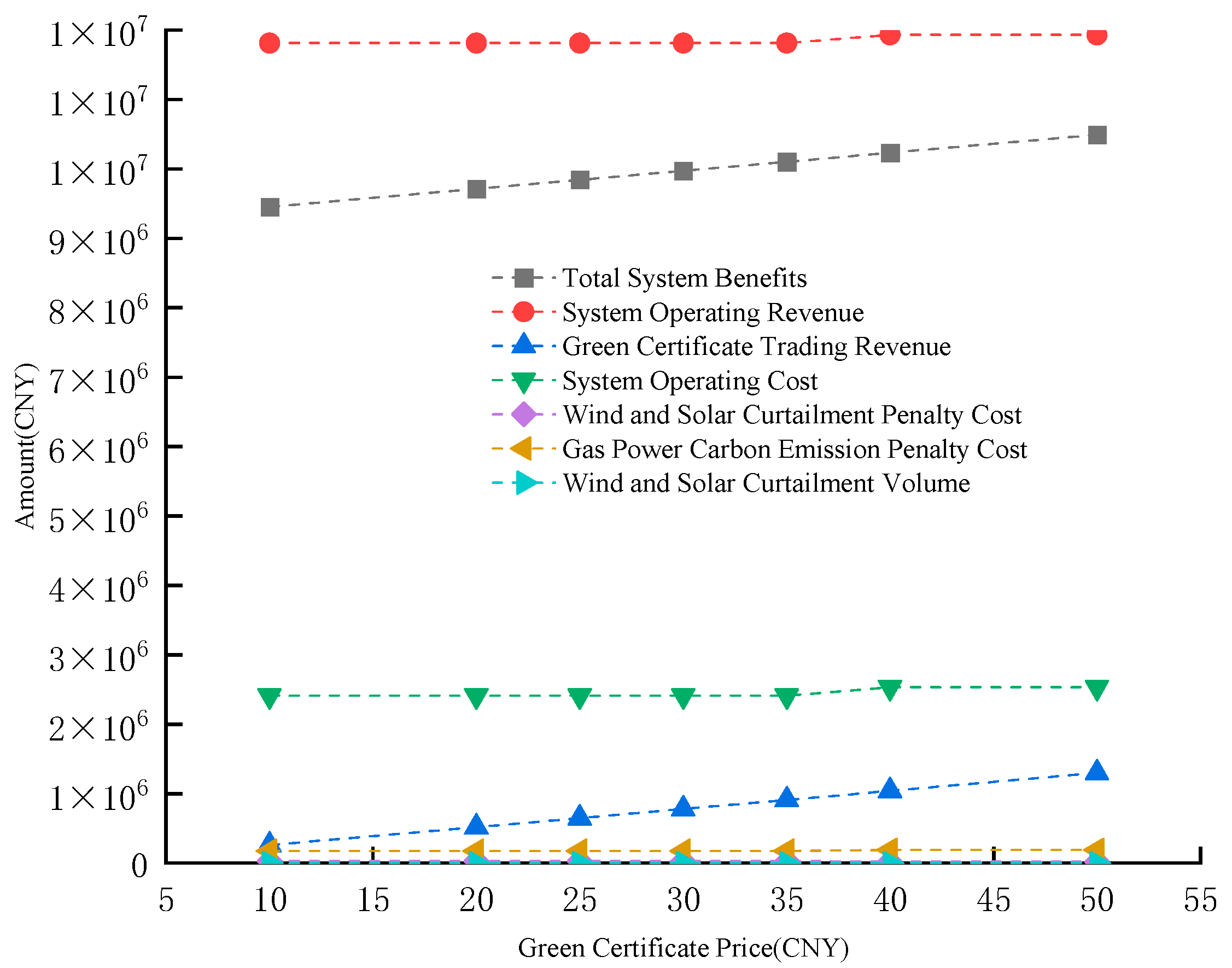
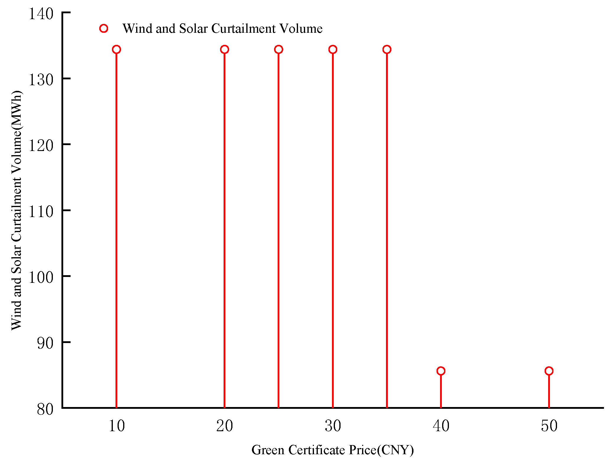
- Green Certificate Price on System Economic Indicators
- (5)
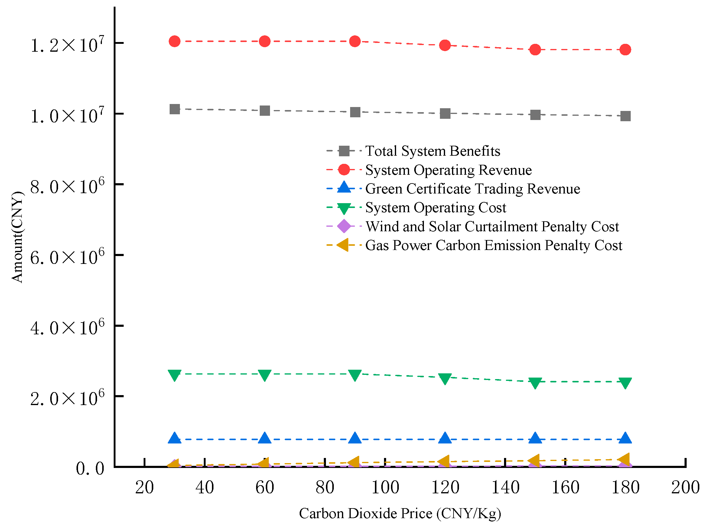
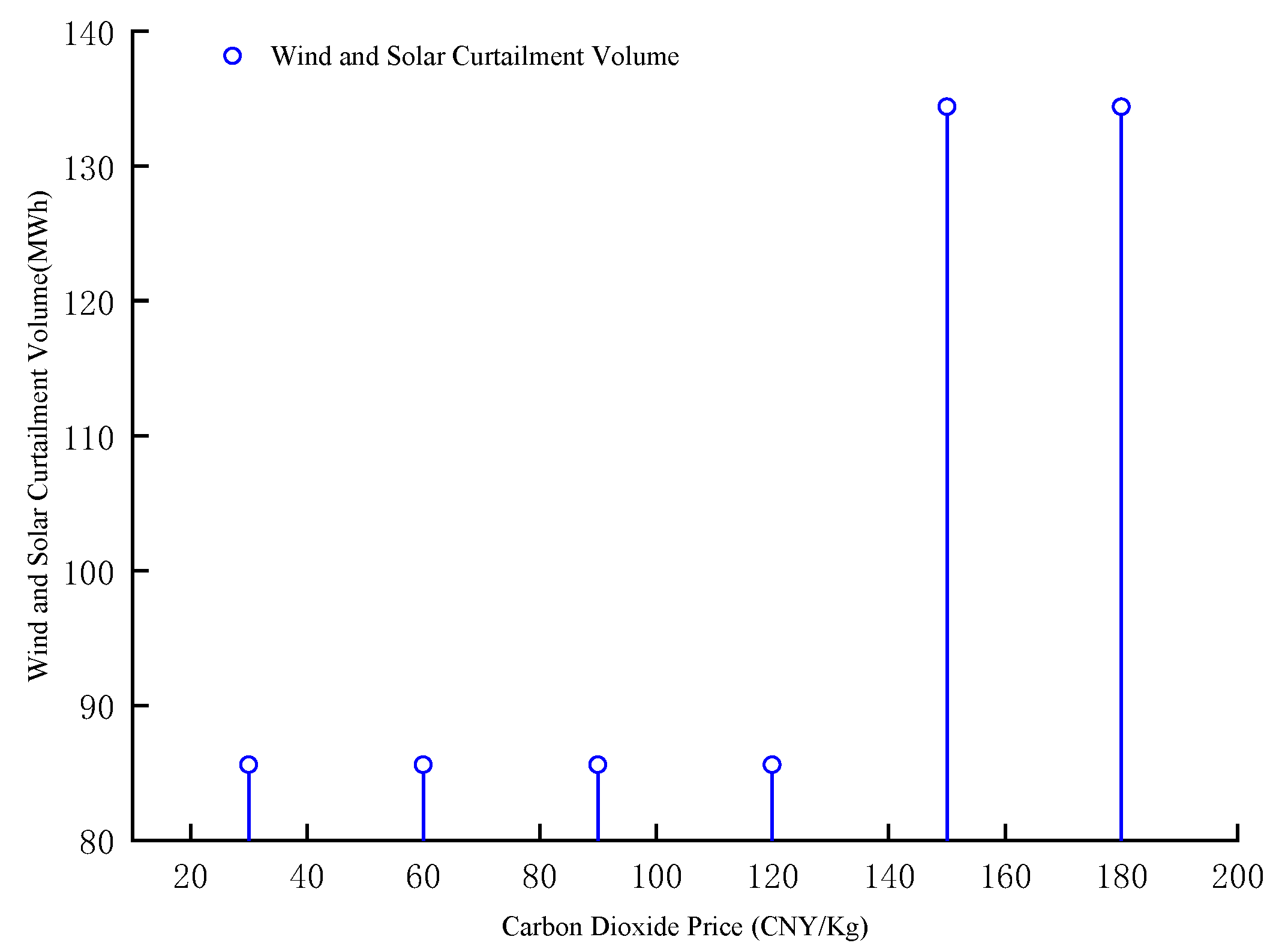
- Carbon Dioxide Price on System Economic Indicators
- (6)
- Carbon Dioxide Price on System Economic Indicators
5. Conclusions, Policy Implications and Limitations
5.1. Conclusions
5.2. Policy Implications and Limitations
Funding
Data Availability Statement
Acknowledgments
Conflicts of Interest
Appendix A
Appendix B
- ①
- The code is as follows: Define a function.
| function f = Efficiency(x) |
| T = length(x); |
| a = 0.361; |
| k = −0.000842; |
| for t = 1:T |
| f(t) = a*exp(k*x(t)); |
| end |
| end |
- ②
- Modeling and Solving.
| clc |
| clear |
| close all |
| T=24; |
| NM=4; |
| E=ones(1,T); |
| E=1*10^3.*[0.43 0.43 0.43 0.43 0.43 0.43 0.43 0.79 0.79 0.79 0.79 1.16 1.16 1.16 0.79 0.79 0.79 0.79 1.16 1.16 1.16 1.16 0.41 0.41]; |
| PL=ones(1,T); |
| PL=2.65.*[302.4509804 299.0196078 298.4509804 291.0294118 292.745098 294.754902 295.0490196 320.7843137 413.9705882 424.2647059 420.8333333 462.5 462.5 377.9411765 439.7058824 434.5588235 410.5392157 459.0686275 450.4901961 435.0490196 424.754902 416.1764706 414.4607843 416.1764706]; |
| row_w=30 |
| row_pv=30 |
| TS=2; |
| TO=2; |
| G_chushi=[0.66 0.73 0.81 0.90 1.00 1.12 1.24 1.38 1.53 1.68 1.85 2.04 2.24 2.46 2.71 2.98 3.28]; |
| G=G_chushi(1,9); |
| LHV=9.082e-03; |
| eata=ones(NM,T); |
| Temp=[20 19 18 17 17 17 20 22 24 26 28 30 32 32 32 31 30 29 28 27 26 24 22 20]; |
| nj_n1=Efficiency(Temp); |
| eata=nj_n1.*ones(NM,T); |
| Pg_m_min=ones(1,NM); |
| Pg_m_max=ones(1,NM); |
| Pg_m_max=[385,385,800,800]; |
| Pg_m_min=0.3.*Pg_m_max; |
| deta_g=ones(1,NM); |
| deta_g=[350,350,450,450]; |
| Kw=0.03*10^3; |
| Kpv=0.04*10^3; |
| S=3.16e+04; |
| Cp_w=230; |
| Cp_pv=230; |
| Pw_xishu=[0.41 0.59 0.51 0.64 0.69 0.57 0.49 0.41 0.22 0.15 0.09 0.22 0.23 0.16 0.28 0.35 0.29 0.25 0.18 0.16 0.18 0.29 0.36 0.46 |
| 0.45 0.43 0.50 0.50 0.49 0.55 0.60 0.61 0.55 0.43 0.44 0.40 0.36 0.38 0.39 0.38 0.43 0.38 0.45 0.57 0.52 0.39 0.39 0.48 |
| 0.31 0.33 0.29 0.35 0.34 0.34 0.32 0.32 0.22 0.19 0.22 0.18 0.20 0.24 0.20 0.24 0.20 0.16 0.19 0.24 0.23 0.16 0.14 0.11 |
| 0.30 0.12 0.10 0.16 0.11 0.11 0.17 0.15 0.15 0.17 0.18 0.17 0.18 0.20 0.19 0.22 0.26 0.37 0.50 0.45 0.47 0.48 0.38 0.38]; |
| Ppv_xishu=[0 0 0 0 0 0.025641026 0.025641026 0.096153846 0.198717949 0.346153846 0.602564103 0.621794872 0.538461538 0.602564103 0.570512821 0.512820513 0.384615385 0.333333333 0.192307692 0.028717949 0 0 0 0 |
| 0 0 0 0 0 0.032051282 0.032051282 0.064102564 0.288461538 0.294871795 0.634615385 0.662820513 0.634615385 0.673076923 0.564102564 0.483333333 0.388461538 0.282051282 0.166666667 0.028846154 0 0 0 0 |
| 0 0 0 0 0 0.032051282 0.025641026 0.070512821 0.211538462 0.528205128 0.583333333 0.616666667 0.66025641 0.532051282 0.548717949 0.492307692 0.337179487 0.265384615 0.137179487 0.023589744 0 0 0 0 |
| 0 0 0 0 0 0.019230769 0.012820513 0.064102564 0.224358974 0.461538462 0.480769231 0.647435897 0.621794872 0.65 0.429487179 0.435897436 0.282051282 0.224358974 0.153846154 0.108974359 0 0 0 0]; |
| PW=2240; |
| Pw_fore=Pw_xishu(1,:).*PW; |
| PPV=1490; |
| Ppv_fore=Ppv_xishu(4,:).*PPV; |
| rw=0.15;rpv=0.05; |
| fai_g=0.02; |
| fai_w=0.02; |
| fai_pv=0.02; |
| Pd_max=2500; |
| deta_Pd=150; |
| K_CO2=150*10^(-3); |
| p_CO2=0.339; |
| C_CO2=K_CO2.*p_CO2.*10^(3); |
| Pw=sdpvar(1,T); |
| Ppv=sdpvar(1,T); |
| Pg=sdpvar(NM,T); |
| Pw_a=sdpvar(1,T); |
| Ppv_a=sdpvar(1,T); |
| Ug=binvar(NM,T); |
| Ps=sdpvar(1,T); |
| Rg=sdpvar(NM,T); |
| Pg_sum=sdpvar(1,1); |
| P_price=1*10^3.*[0.3515 0.3514 0.3634 0.3497 0.3205 0.3729 0.2772 0.3685 0.3717 0.3723 0.3035 0.4048 0.378 0.4153 0.3693 0.3737 0.3981 0.4471 0.3551 0.4012 0.3796 0.3993 0.3346 0.2978 0.3247 0.2595 0.4505 0.414 0.3358 0.3363 0.4198]; |
| P_price=sort(P_price); |
| P_price=1*10^3.*[0.259500000000000,0.277200000000000,0.297800000000000,0.303500000000000,0.320500000000000,0.32 4700000000000,0.334600000000000,0.335800000000000,0.336300000000000,0.349700000000000,0.351400000000000,0.3515 00000000000,0.355100000000000,0.363400000000000,0.368500000000000,0.369300000000000,0.371700000000000,0.372300 000000000,0.372900000000000,0.373700000000000,0.378000000000000,0.379600000000000,0.398100000000000,0.39930000 0000000,0.401200000000000,0.404800000000000,0.414000000000000,0.415300000000000,0.419800000000000,0.4471000000 00000,0.450500000000000]; |
| P_price=1*10^3.*[0.3796,0.3981,0.3993,0.4012,0.4048,0.4140,0.4198 0.65 0.7 0.8]; |
| Cw=P_price(1,4); |
| Cpv=Cw; |
| Cg=Cw; |
| C=[]; |
| for t=1:T |
| C=[C,Pw(1,t).*(1-fai_w)+Ppv(1,t).*(1-fai_pv)+sum(Pg(:,t).*(1-fai_g))==Ps(1,t), |
| Pw_fore(1,t)==Pw(1,t)+Pw_a(1,t), |
| Ppv_fore(1,t)==Ppv(1,t)+Ppv_a(1,t), |
| Pw(1,t)>=0, |
| Ppv(1,t)>=0, |
| Pw_a(1,t)>=0, |
| Ppv_a(1,t)>=0, |
| ]; |
| for m=1:NM |
| C=[C, Ug(m,t).*Pg_m_min(1,m)<=Pg(m,t)<=Ug(m,t).*Pg_m_max(1,m), |
| ]; |
| end |
| end |
| C=[C,Ps<=Pd_max, |
| Pg_sum==sum(sum(Pg)), |
| ]; |
| for t=2:T |
| C=[C,-deta_Pd<=Ps(1,t)-Ps(1,t-1)<=deta_Pd,]; |
| end |
| for t=2:T |
| for m=1:NM |
| C=[C,Pg(m,t)-Pg(m,t-1)+Ug(m,t-1).*(Pg_m_min(1,m)-deta_g(1,m))+Ug(m,t).*(Pg_m_max(1,m)-Pg_m_min(1,m))<=Pg_m_max(1,m), |
| Pg(m,t-1)-Pg(m,t)+Ug(m,t).*(Pg_m_min(1,m)-deta_g(1,m))+Ug(m,t-1).*(Pg_m_max(1,m)-Pg_m_min(1,m))<=Pg_m_max(1,m), |
| ]; |
| k=t; |
| T_new1=min(t+TS-1,T); |
| T_new2=min(t+TO-1,T); |
| C=[C,sum(1-Ug(m,k:T_new1))>=TS.*(Ug(m,t-1)-Ug(m,t)), |
| sum(Ug(m,k:T_new2))>=TO.*(Ug(m,t)-Ug(m,t-1)), |
| ]; |
| end |
| end |
| Y=binvar(NM,T); |
| sum_qd=sdpvar(1,m); |
| for m=1:NM |
| sum_qd(1,m)=0; |
| for t=2:T |
| sum_qd(1,m)=sum_qd(1,m)+Ug(m,t).*S-Y(m,t-1).*S; |
| C=[C,Y(m,t)<=Ug(m,t), |
| Y(m,t-1)<=Ug(m,t-1), |
| Ug(m,t)>=Ug(m,t-1)-(1-Ug(m,t)), |
| ]; |
| end |
| end |
| Pg_max_t=sdpvar(NM,T); |
| for t=1:T |
| C=[C,sum(Rg(:,t))>=rw.*Pw_fore+rpv.*Ppv_fore, |
| ]; |
| for m=1:NM |
| C=[C, Rg(m,t)<=Pg_max_t(m,t)-Pg(m,t), |
| 0<=Rg(m,t)<=deta_g(1,m), |
| Pg_max_t(m,t)<=Pg_m_max(1,m), |
| ]; |
| end |
| end |
| chengben=sdpvar(NM,T); |
| sum_chengben=sdpvar(1,T); |
| for t=1:T |
| for m=1:NM |
| chengben(m,t)=sum(G.*Pg(m,t)/(LHV.*eata(1,t))); |
| end |
| sum_chengben(1,t)=sum(chengben(:,t)); |
| end |
| f1=sum(Cw.*Pw)+sum(Cpv.*Ppv)+sum(Cg.*sum(Pg)); |
| f2=sum(row_w.*Pw)+sum(row_pv.*Ppv); |
| f3=sum(Kw.*Pw)+sum(Kpv.*Ppv)+sum(sum_chengben)+sum(sum_qd); |
| Pg_chengben=sum(sum_chengben)+sum(sum_qd); |
| Pg_shouru=sum(Cg.*sum(Pg)); |
| f4=sum(Cp_w.*Pw_a)+sum(Cp_pv.*Ppv_a); |
| f5=C_CO2.*sum(sum(Pg)); |
| F=f1+f2-f3-f4-f5; |
| F1=-F; |
| ops=sdpsettings('verbose',1,'debug',1,'solver','cplex','savesolveroutput',1,'savesolverinput',1); |
| ops.cplex.mip.tolerances.mipgap=1e-6; |
| ops.cplex.exportmodel='gas_wind_pv.lp'; |
| F1_result=optimize(C,F1,ops); |
| F1=value(F1); |
| if F1_result.problem == 0 |
| disp([' Solution found ',' F=', num2str(-F1)]); |
| else |
| error(' Solving error '); |
| end |
References
- Huang, Z.; Huang, Y.; Zhang, S. The possibility and improvement directions of achieving the paris agreement goals from the perspective of climate policy. Sustainability 2024, 16, 4212. [Google Scholar] [CrossRef] [Scilit]
- Liu, J.; Zhang, P.; Wang, X. Exploring the Mechanisms and Pathways Through Which the Digital Transformation of Manufacturing Enterprises Enhances Green and Low-Carbon Performance Under the “Dual Carbon” Goals. Sustainability 2025, 17, 1162. [Google Scholar] [CrossRef] [Scilit]
- Duan, W.; Zhao, W.; Xu, D. Study on the pathway of energy transition in Inner Mongolia under the “dual carbon” goal. Heliyon 2024, 10, e39764. [Google Scholar] [CrossRef] [Scilit]
- Yang, B.; Li, Y.; Yao, W.; Jiang, L.; Zhang, C.; Duan, C.; Ren, Y. Optimization and control of new power systems under the dual carbon goals: Key Issues, advanced techniques, and perspectives. Energies 2023, 16, 3904. [Google Scholar] [CrossRef] [Scilit]
- Naseem, K.; Khalid, F.; Qin, F.; Zhu, J.; Suo, G.; Shah, B.A. The catalytic role of cubic iron oxide coated graphene oxide for hydrogen generation via hydrolysis of Magnesium. Renew. Energy 2025, 256, 124515. [Google Scholar] [CrossRef] [Scilit]
- Jiang, Q.; Yin, Z. The optimal path for China to achieve the “Dual Carbon” target from the perspective of energy structure optimization. Sustainability 2023, 15, 10305. [Google Scholar] [CrossRef] [Scilit]
- Yang, B.; Duan, J.; Liu, Z.; Jiang, L. Exploring Sustainable Development of New Power Systems under Dual Carbon Goals: Control, Optimization, and Forecasting. Energies 2024, 17, 3909. [Google Scholar] [CrossRef] [Scilit]
- Milligan, M.; Frew, B.; Kirby, B.; Schuerger, M.; Clark, K.; Lew, D.; Denholm, P.; Zavadil, B.; O’Malley, M.; Tsuchida, B. Alternatives no more: Wind and solar power are mainstays of a clean, reliable, affordable grid. IEEE Power Energy Mag. 2015, 13, 78–87. [Google Scholar] [CrossRef] [Scilit]
- Adefarati, T.; Sharma, G.; Bokoro, P.N.; Kumar, R. Advancing renewable-dominant power systems through internet of things and artificial intelligence: A comprehensive review. Energies 2025, 18, 5243. [Google Scholar] [CrossRef] [Scilit]
- Mo, D.; Li, Q.; Lu, Y. Wind solar thermal storage collaborative low-carbon economic dispatch that adapts to wind solar volatility and dynamic peak shaving capacity of energy storage. Energy Storage Sci. Technol. 2025, 14, 1701. [Google Scholar]
- Peng, N.; Miao, J.; Hu, S.; Zhao, L.; Wang, Y.; Meng, F.; Yi, Y.; Zheng, Z. Quantitative Evaluation Of The Complementarity And Capacity Ratio Of Large-scale Wind Power And Photovoltaic. J. Appl. Sci. Eng. 2025, 28, 1243–1252. [Google Scholar]
- Alizadeh, M.I.; Moghaddam, M.P.; Amjady, N.; Siano, P.; Sheikh-El-Eslami, M.K. Flexibility in future power systems with high renewable penetration: A review. Renew. Sustain. Energy Rev. 2016, 57, 1186–1193. [Google Scholar] [CrossRef] [Scilit]
- Impram, S.; Nese, S.V.; Oral, B. Challenges of renewable energy penetration on power system flexibility: A survey. Energy Strategy Rev. 2020, 31, 100539. [Google Scholar] [CrossRef] [Scilit]
- Liu, L.; Wang, Z.; Wang, Y.; Wang, J.; Chang, R.; He, G.; Tang, W.; Gao, Z.; Li, J.; Liu, C. Optimizing wind/solar combinations at finer scales to mitigate renewable energy variability in China. Renew. Sustain. Energy Rev. 2020, 132, 110151. [Google Scholar] [CrossRef] [Scilit]
- Jurasz, J.; Guezgouz, M.; Campana, P.E.; Kaźmierczak, B.; Kuriqi, A.; Bloomfield, H.; Hingray, B.; Canales, F.A.; Hunt, J.D.; Sterl, S. Complementarity of wind and solar power in North Africa: Potential for alleviating energy droughts and impacts of the North Atlantic Oscillation. Renew. Sustain. Energy Rev. 2024, 191, 114181. [Google Scholar] [CrossRef] [Scilit]
- Zhang, H.; Lu, Z.; Hu, W.; Wang, Y.; Dong, L.; Zhang, J. Coordinated optimal operation of hydro–wind–solar integrated systems. Appl. Energy 2019, 242, 883–896. [Google Scholar] [CrossRef] [Scilit]
- Zhang, J.; Wang, H.; Fan, C.; Hu, J.; Zhang, X. Hydro–Wind–PV–Integrated Operation Optimization and Ultra-Short-Term HESS Configuration. Electronics 2024, 13, 4778. [Google Scholar] [CrossRef] [Scilit]
- Li, X.; Wang, K.; Xu, M.; Fu, M.; Miao, S. Environmental and economic dispatching strategy for power system with the complementary combination of wind-solar-hydro-thermal-storage multiple sources. Front. Energy Res. 2024, 12, 1338657. [Google Scholar] [CrossRef] [Scilit]
- Chen, Y.; Zhang, J.; Wang, F.; Zhang, J.; Wu, W.; Li, H. Study on Carbon Emission Reduction Strategy of CCUS Technology in Natural Gas Supply Chain Considering Government Subsidies. Processes 2025, 13, 550. [Google Scholar] [CrossRef] [Scilit]
- Varghese, S.; Dalvi, S.; Narula, A.; Webster, M. The impacts of distinct flexibility enhancements on the value and dynamics of natural gas power plant operations. IEEE Trans. Power Syst. 2021, 36, 5803–5813. [Google Scholar] [CrossRef] [Scilit]
- Nyangon, J.; Byrne, J. Estimating the impacts of natural gas power generation growth on solar electricity development: PJM’s evolving resource mix and ramping capability. Wiley Interdiscip. Rev. Energy Environ. 2023, 12, e454. [Google Scholar] [CrossRef] [Scilit]
- Mohammad, N.; Mohamad Ishak, W.W.; Mustapa, S.I.; Ayodele, B.V. Natural gas as a key alternative energy source in sustainable renewable energy transition: A mini review. Front. Energy Res. 2021, 9, 625023. [Google Scholar] [CrossRef] [Scilit]
- Akbar Akhgari, P.; Kamalan, H. Economical–environmental evaluation of natural gas and renewable energy systems. Int. J. Energy Res. 2013, 37, 1550–1561. [Google Scholar] [CrossRef] [Scilit]
- Alavijeh, H.S.; Kiyoumarsioskouei, A.; Asheri, M.; Naemi, S.; Alavije, H.S.; Tabrizi, H.B. Greenhouse gas emission measurement and economic analysis of Iran natural gas fired power plants. Energy Policy 2013, 60, 200–207. [Google Scholar] [CrossRef] [Scilit]
- Vandani, A.M.K.; Joda, F.; Boozarjomehry, R.B. Exergic, economic and environmental impacts of natural gas and diesel in operation of combined cycle power plants. Energy Convers. Manag. 2016, 109, 103–112. [Google Scholar] [CrossRef] [Scilit]
- Clark, S.; McGregor, C.; Van Niekerk, J. Using liquefied petroleum gas to reduce the operating cost of the Ankerlig peaking power plant in South Africa. J. Energy S. Afr. 2022, 33, 15–23. [Google Scholar] [CrossRef] [Scilit]
- Qingmin, M.; Zhonglin, Z.; Fangwei, P. Development Trends of Natural Gas Resources and Gas-Fired Power Generations in China. Environ. Prog. Sustain. Energy 2016, 35, 853–858. [Google Scholar] [CrossRef] [Scilit]
- Shabazbegian, V.; Ameli, H.; Ameli, M.T.; Strbac, G. Stochastic optimization model for coordinated operation of natural gas and electricity networks. Comput. Chem. Eng. 2020, 142, 107060. [Google Scholar] [CrossRef] [Scilit]
- Shabazbegian, V.; Ameli, H.; Ameli, M.T.; Strbac, G.; Qadrdan, M. Co-optimization of resilient gas and electricity networks; a novel possibilistic chance-constrained programming approach. Appl. Energy 2021, 284, 116284. [Google Scholar] [CrossRef] [Scilit]
- Stanley, A.P.; King, J.; Barker, A.; Guittet, D.; Hamilton, W.; Bay, C.; Fleming, P.; Sinner, M. Multi-timescale wind-based hybrid energy systems. J. Phys. Conf. Ser. 2022, 2265, 042062. [Google Scholar] [CrossRef] [Scilit]
- Mirzaei, M.A.; Nazari-Heris, M.; Mohammadi-Ivatloo, B.; Marzband, M.; Anvari-Moghaddam, A. Two-stage stochastic day-ahead market clearing in gas and power networks integrated with wind energy. J. Renew. Energy Environ. 2019, 5, 53–59. [Google Scholar]
- Miller, I.; Gençer, E.; O’Sullivan, F.M. A general model for estimating emissions from integrated power generation and energy storage. Case study: Integration of solar photovoltaic power and wind power with batteries. Processes 2018, 6, 267. [Google Scholar] [CrossRef] [Scilit]
- Sharifi, V.; Abdollahi, A.; Rashidinejad, M.; Heydarian-Forushani, E.; Alhelou, H.H. Integrated electricity and natural gas demand response in flexibility-based generation maintenance scheduling. IEEE Access 2022, 10, 76021–76030. [Google Scholar] [CrossRef] [Scilit]
- Sleiman, A.; Su, W. Combined K-means clustering with neural networks methods for PV short-term generation load forecasting in electric utilities. Energies 2024, 17, 1433. [Google Scholar] [CrossRef] [Scilit]
- Miraftabzadeh, S.M.; Colombo, C.G.; Longo, M.; Foiadelli, F. K-means and alternative clustering methods in modern power systems. IEEE Access 2023, 11, 119596–119633. [Google Scholar] [CrossRef] [Scilit]
- He, Z.; Liu, C.; Wang, Y.; Wang, X.; Man, Y. Optimal operation of wind-solar-thermal collaborative power system considering carbon trading and energy storage. Appl. Energy 2023, 352, 121993. [Google Scholar] [CrossRef] [Scilit]



| Indicator Set | Symbol | Meaning |
| Set of scheduling time, | ||
| Set of power units, |
| Gas–Wind–Solar Combined Generation Parameters | Symbol | Meaning | |
| Decision Variables | Output of gas power unit i at time t | ||
| Output of wind farm at time t | |||
| Output of solar power station at time t | |||
| Wind power curtailment at time t | |||
| Solar power curtailment at time t | |||
| Total power delivery at time t | |||
| Start-up/shut-down state variable of gas power unit i at time t | |||
| Model Parameters | Gas power grid electricity price | ||
| Wind power grid electricity price | |||
| Green certificate trading price for wind power | |||
| Green certificate quota coefficient per unit of wind power | |||
| Green certificate trading price for solar power | |||
| Unit operation cost of wind power | |||
| Unit operation cost of solar power | |||
| Start-up/shut-down cost of gas power unit | |||
| Natural gas price | |||
| Lower heating value of natural gas | |||
| Average efficiency of gas power unit i | |||
| Scheduling time scale | |||
| Reserve capacity demand ratio of gas power unit i | |||
| Maximum output of gas power unit i at time t | |||
| Maximum technical output of gas power unit i | |||
| Ramping rate of gas power unit i | |||
| Wind farm output coefficient at time t (based on local wind forecast) | |||
| Solar farm output coefficient at time t (based on local solar forecast) | |||
| Installed capacity of wind farm | |||
| Installed capacity of solar farm | |||
| Minimum output of gas power unit i | |||
| Maximum output of gas power unit i | |||
| Continuous operation time of gas power unit i at time t − 1 | |||
| Continuous shut-down time of gas power unit i at time t − 1 | |||
| Minimum run-time of gas power unit i | |||
| Minimum shut-down time of gas power unit i | |||
| Wind power predicted output at time t | |||
| Solar power predicted output at time t | |||
| Meanings | Wind Power | Photovoltaic Power |
|---|---|---|
| The reserve capacity demand ratio | 0.15 | 0.05 |
| The installed capacity | 2240 MW | 1490 MW |
| The price for green certificate trading | 30 CNY/MWh | 30 CNY/MWh |
| The green certificate quota coefficient | 1 | 1 |
| The penalty cost coefficient | 230 CNY/MWh | 230 CNY/MWh |
| The self-use electricity rate | 2% | 2% |
| The transmission capacity of the export line | 2500 MW | 2500 MW |
| The power fluctuation range | ±150 MW/h | ±150 MW/h |
| The grid-connected price | 401.2 CNY/MWh | 401.2 CNY/MWh |
| The unit operation cost | 30 CNY/MWh | 40 CNY/MWh |
| The scheduling period | 24 h | 24 h |
| The time interval of scheduling period | 1 h | 1 h |
| Meanings | F-Class | H-Class |
|---|---|---|
| The reserve capacity demand ratio | 1.4% | 1.4% |
| The transmission capacity of the export line | 2500 MW | 2500 MW |
| The power fluctuation range | ±150 MW/h | ±150 MW/h |
| The grid-connected price | 401.2 CNY/MWh | 401.2 CNY/MWh |
| The scheduling period | 24 h | 24 h |
| The time interval of scheduling period | 1 h | 1 h |
| The minimum output of the gas turbines | 115.5 MW | 240 MW |
| The ramp-up rates | 250 MW | 480 MW |
| The start–stop duration constraint | 2 h | 2 h |
| The startup–shutdown cost | 31,600 CNY | 31,600 CNY |
| The carbon emission penalty cost | 50.85 CNY/MWh | 50.85 CNY/MWh |
| The natural gas price | 1.53 CNY/m3 | 1.53 CNY/m3 |
| The lower heating value (LHV) of natural gas | 9.082 × 10⁻³ MWh/m3 | 9.082 × 10⁻³ MWh/m3 |
| Installed Capacity × Quantity (MW) | 385 × 2 | 800 × 2 |
| Economic Indicator | System Total Economic Benefit | System Operating Income | Green Certificate Trading Income | System Operating Cost | Wind and Solar Curtailment Penalty Cost | Gas Power Carbon Emission Penalty Cost |
|---|---|---|---|---|---|---|
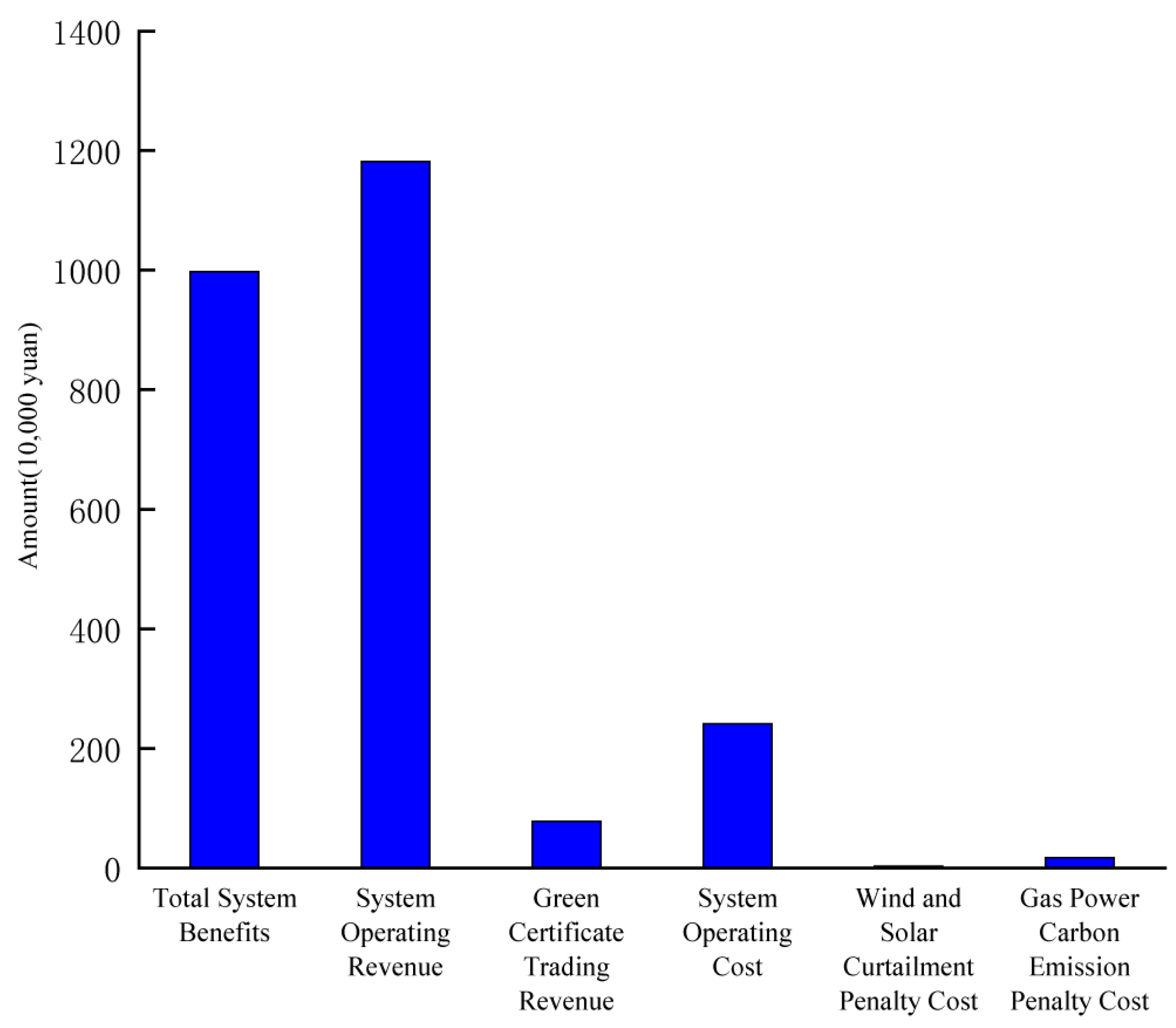
| Amount (in 10,000 yuan) | 997.34 | 1181.82 | 77.95 | 241.14 | 3.09 | 17.60 |
| Type | Scenario | Total System Benefits | System Operating Revenue | Green Certificate Trading Revenue | System Operating Cost | Wind and Solar Curtailment Penalty Cost | Gas Power Carbon Emission Penalty Cost |
|---|---|---|---|---|---|---|---|
| Wind Power (10,000 yuan) | 1 | 997.34 | 1181.22 | 77.95 | 241.14 | 3.09 | 17.60 |
| 2 | 1264.67 | 1390.93 | 97.28 | 208.40 | 3.74 | 11.40 | |
| 3 | 785.09 | 893.20 | 61.17 | 154.83 | 4.93 | 9.52 | |
| 4 | 792.80 | 920.88 | 62.44 | 171.58 | 8.07 | 10.87 | |
| Photovoltaic (10,000 yuan) | 1 | 984.50 | 1161.20 | 76.97 | 231.54 | 5.41 | 16.71 |
| 2 | 997.34 | 1181.22 | 77.95 | 241.14 | 3.09 | 17.60 | |
| 3 | 977.56 | 1183.56 | 76.96 | 258.41 | 4.98 | 19.57 | |
| 4 | 971.13 | 1142.04 | 75.83 | 225.38 | 5.15 | 16.22 |
Disclaimer/Publisher’s Note: The statements, opinions and data contained in all publications are solely those of the individual author(s) and contributor(s) and not of MDPI and/or the editor(s). MDPI and/or the editor(s) disclaim responsibility for any injury to people or property resulting from any ideas, methods, instructions or products referred to in the content. |
© 2025 by the author. Licensee MDPI, Basel, Switzerland. This article is an open access article distributed under the terms and conditions of the Creative Commons Attribution (CC BY) license.
Share and Cite
Wang, F. Study on the Economic Benefits of Gas–Wind–Solar Power Alliance Under Gas Peaking Mode. Energies 2026, 19, 125. https://doi.org/10.3390/en19010125
Wang F. Study on the Economic Benefits of Gas–Wind–Solar Power Alliance Under Gas Peaking Mode. Energies. 2026; 19(1):125. https://doi.org/10.3390/en19010125
Chicago/Turabian StyleWang, Fuping. 2026. "Study on the Economic Benefits of Gas–Wind–Solar Power Alliance Under Gas Peaking Mode" Energies 19, no. 1: 125. https://doi.org/10.3390/en19010125
APA StyleWang, F. (2026). Study on the Economic Benefits of Gas–Wind–Solar Power Alliance Under Gas Peaking Mode. Energies, 19(1), 125. https://doi.org/10.3390/en19010125