Research on Energy Management Strategies for Fuel Cell Hybrid Vehicles Based on Time Classification

Abstract

In order to minimize the carbon emission and energy consumption of fuel cell hybrid vehicles and, at the same time, solve the problem of low accuracy of working condition identification in the working condition identification strategy, this paper proposes an energy management strategy for SUVs on the basis of the working condition identification energy management strategy by using the time classification method. First, the mathematical model of the whole vehicle power system is established, and the driving conditions are constructed using actual collected vehicle driving data. On this basis, the working condition identification model was established, and then the energy management strategy of time working condition classification was established on the basis of the working condition identification model, and the equivalent hydrogen consumption of the two strategies was calculated by the Pontryagin minimization strategy. The results show that the strategy proposed in this paper reduces the equivalent hydrogen consumption by 2.707% compared with the condition identification strategy. This improvement not only greatly improves the energy efficiency of the fuel cell hybrid vehicle but also provides new ideas for the optimization of future energy management strategies.

1. Introduction

Transportation is one of the most significant sources of CO₂ emissions [1]. The transportation sector accounts for approximately 30% of total global CO₂ emissions, with emissions from on-road vehicles reaching nearly 70% [2]. The use of new energy sources and the construction of sustainable transportation systems have been emphasized as the need to mitigate the climate problem is becoming more and more urgent [3]. Moreover, electric vehicles and fuel cell electric vehicles are considered to be the best choice to promote the use of new energy [4]. Among them, the environmental benefits of EVs depend largely on the source of electricity used to charge them; if the electricity is mainly derived from fossil fuels (e.g., coal, natural gas, etc.), the whole-life carbon emissions of EVs may be comparable to or even higher than those of conventional fuel vehicles, as a large amount of carbon emissions have already been generated in the process of coal-fired power generation. On the contrary, if electricity comes mainly from renewable energy sources (e.g., wind, solar, hydro, etc.), the carbon emissions of electric vehicles will be significantly reduced, thus achieving real environmental benefits. However, the stability of their energy supply and large-scale rollout has been limited by the inherent limitations of the intermittent and volatile nature of natural resources. Hydrogen energy is an effective way to achieve large-scale deep decarbonization, and hydrogen production from the electrolysis of water is not only one of the ways to obtain green hydrogen energy but also helps to solve the problem of intermittency and variability in renewable energy sources [5].

Fuel cell vehicles are generally equipped with batteries or supercapacitors to reduce fuel cell size, addressing issues such as soft output characteristics and the inability to recover braking energy [6]. Several automobile companies are currently developing or successfully testing fuel cell hybrid vehicles [7]. Therefore, it is of great significance to carry out reasonable power allocation for fuel cell hybrid vehicles with dual power sources to improve the efficiency and economy of energy utilization to achieve environmentally friendly travel and energy saving and emission reduction.

Currently, the main energy management strategies for hybrid vehicles are rule and optimization-based [8]. Rule-based strategies tend to be used in engineering applications, where rules are formulated by experts based on empirical and historical data to determine the energy allocation of the entire vehicle; however, rule-based strategies are poorly adapted and cannot achieve optimal performance when facing different road conditions [9,10]. The optimization-based strategy is suitable for solving the energy management problems of complex nonlinear systems with better optimization effects, which can be close to or even reach the theoretical optimum [11,12]. Typical optimization algorithms include Dynamic Programming (DP), Convex Optimization (CVX), and Pontryagin’s minimum principle (PMP) [12]. Du Chen et al. [13] proposed a dynamic planning-based optimization method for the energy management strategy of fuel cell hybrid vehicles, which improves the rule-based strategy through the distribution scheme of the dynamic planning strategy. The results showed that hydrogen consumption was significantly reduced compared with the pre-improvement period. According to Wang Xu et al. [14], a convex optimization algorithm was proposed to optimize the motor model and power battery parameters of an electric vehicle, an optimization algorithm using double-loop dynamic programming, and a nonlinear optimization approach. Xu Liu et al. [15] compared Dynamic programming (DP), PMP, Charge Depletion Charge Maintenance (CDCS), and hybrid strategies and showed that although the PMP strategy leads to a 1.4% higher operating cost than DP, it is suitable for real-time control systems. The energy performance of the PMP strategy raises the question of how to continue reducing energy consumption and performing complex power allocation to vehicles based on the PMP energy management strategy.

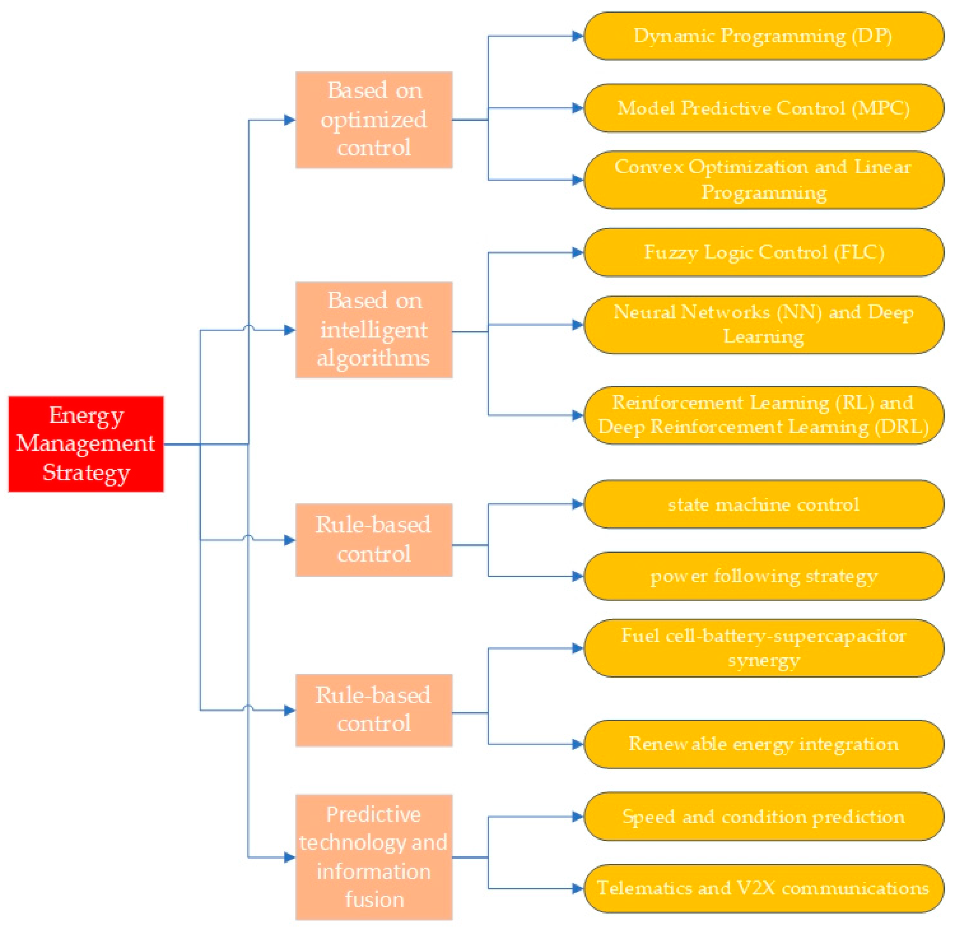
However, there are still some challenges with current energy management strategies and one of the challenges is to optimize the setup and design of appropriate controllers because of the proper integration of systems in the vehicle [16]. Figure 1 shows the classification of energy management strategies. Since most of the energy management strategy studies are limited to simulation, they are not validated by real-time or real experimental applications [17]; therefore, future EMS simulations must be validated through real-time applications or experimental setups.

To address this issue, numerous researchers have suggested a condition identification method for energy management strategies to enhance vehicle dynamics and efficiency, which has online control and offline optimization functions for real-time applications [15,18]. Zhang Xu et al. [19] combined the state identification algorithm with a fuzzy controller optimized based on the particle swarm algorithm, which resulted in an effective reduction in energy consumption and prolongation of battery life compared with three energy management strategies without state identification. Ravey et al. [20] used five feature parameters, namely average speed, number of stops, stopping time, acceleration, deceleration, and the weighted product sum of these five feature parameters as input parameters, and used a dynamic clustering method for driving condition identification. However, work condition recognition also has some limitations, and both real-time and recognition accuracies are challenging [19].

To reduce the impact of poor real-time and low precision of working condition identification on hydrogen consumption, formulating a more optimal power allocation energy management strategy has become a key issue. Hou Z et al. [21] established a working condition identification model integrating Random Forest and Support Vector Machine and optimized the logical threshold for each working condition based on the whale algorithm, which significantly improved the adaptability of the rule-based strategy to the working conditions. Guo He et al. [22] used a working condition identification method based on Euclidean proximity, combined with an adaptive wavelet transform to perform power allocation, which significantly reduced the current and voltage fluctuations in the battery–supercapacitor hybrid energy storage system. Xie He et al. [23] proposed a working condition determination method combining variable-scale time window identification and prediction, which combined statistical methods to determine the optimal switching time thresholds for the two models and improved the accuracy of online identification by 21.73%. The control parameters of energy management strategies based on rules or instantaneous optimization are optimized for typical working conditions, and the online identification model of working conditions is established by combining other algorithms, which can improve the accuracy of working condition identification. The coupling of the working condition information with the energy management strategy can achieve the on-line adjustment of the control parameters based on the working conditions. Then, by coupling the working condition information with the energy management strategy, the online adjustment of the control parameters based on the working conditions can be achieved, thus improving the robustness of the strategy and ultimately achieving the purpose of improving the economy of hydrogen consumption. Therefore, this study proposes a time-classified energy management strategy that incorporates work condition identification.

Vehicle speed data were then collected for two time periods, 08–09 a.m. during the peak traffic flow period and 10–11 a.m. during the low traffic flow period for an entire year, and these data were preprocessed for each time period. Because there is also variability in the power distribution and different hydrogen consumption for different types of working conditions, the speed for each time period was clustered and analyzed to obtain three types of working conditions: urban conditions, suburban conditions, and high-speed conditions. At that time, attributes of time were attached to the different types of working conditions. After obtaining the different types of working conditions, the globally optimal covariate λ for each working condition was determined according to the PMP strategy and target shooting method. Simultaneously, after obtaining each working condition, it is necessary to construct a comprehensive working condition, establish a working condition identification model, and calculate the global minimum equivalent hydrogen consumption of the identified online comprehensive working condition based on the simulation of PMP. Energy management strategy based on time classification is first based on PMP and the target-hitting method to solve the optimal covariate for each time period. Because the integrated operating conditions are offline, to match the actual operating conditions better, it is necessary to obtain the online integrated operating conditions based on condition identification. When simulating the online integrated conditions based on the PMP strategy, the optimal covariates at the current time were used to replace the covariates corresponding to each condition in the condition identification. Finally, the entire vehicle was modeled using MATLAB(2022b) software and simulated using MATLAB for verification.

Due to the poor real-time performance of the work condition recognition strategies studied by the original scholars, the blurring of work condition boundaries leads to model misclassification or inaccurate classification, dynamic changes in work conditions may lead to lagging or inaccurate recognition results, and the problem of multi-condition coupling leads to the difficulty of the model in accurately distinguishing and recognizing the coupled work conditions [24]. Therefore, it is necessary to propose a new method to solve these problems. Therefore, this paper proposes an energy management strategy based on time classification, which has not been studied by any scholars so far. Compared with the method based on condition identification, the equivalent hydrogen consumption of the time-based classification method is 2.707% lower than that of the method based on condition identification; this improvement not only significantly improves the energy efficiency of fuel cell hybrid vehicles but also removes the work condition identification errors because of work condition identification, and finally provides new ideas for optimizing future energy management strategies. The energy management strategy for fuel cell hybrid electric vehicles around this method is desirable in meeting the dynamic economy. The condition identification-based approach processes time-stamped speed data and then constructs time-stamped conditions to constitute a time condition. In this paper, we categorize the conditions based on the speeds in a time period, and all speed data in a time period are classified into three conditions: urban, suburban, and highway. Moreover, time classification means dividing a longer time period into several shorter time periods, and then calculating the covariates (similar to the equivalent factor) for each time period and each working condition separately, and then calculating the equivalent hydrogen consumption based on the MATLAB simulation. A large speed dataset is needed in this strategy because the prediction model has to be trained for the working condition identification model, and at the same time, in order to make the time classification strategy have the vehicle speed of the whole year time, which is a more comprehensive dataset, so we used vehicle driving data information of the whole year throughout the simulation process, and at the same time, modeling and experimental tests on the power cell and the fuel cell were carried out to validate the modeling. The remaining sections are organized as follows. Section 2 describes the powertrain configuration and system modeling. Section 3 presents the energy management strategy based on operating condition identification and time classification. Section 4 presents the simulation, validation, and analysis of the results. Section 5 presents the conclusion.

2. Fuel Cell Hybrid Vehicle Model

2.1. Powertrain Configuration

Prior to designing the energy management controller, it was necessary to determine the vehicle configuration and complete parameter matching and modeling of the selected components. The fuel cell vehicle studied in this paper is an FCS + PB structural model. It can charge a power battery, which can solve the problem that fuel cell braking energy cannot be recovered. The drive system arrangement is presented in Figure 2. In addition to the fuel cell and the power cell, the system also includes components such as the vehicle controller (VCU), motor controller (MCU), unidirectional DC converter, and drive motor. Among them, for the unidirectional DC/DC converter at the same power fluctuation, the voltage fluctuation in the low-voltage side of the converter will be lower at the same time using unidirectional DC/DC and can obtain a more stable voltage. This structure is more economical and reliable, and power cell technology is mature, with a more balanced performance in all aspects [5]. The whole vehicle model in this paper is based on a pure electric front-drive car as a prototype after secondary development. The prototype is front-drive, in order to save costs, as far as possible to minimize the structural changes to the original car, and the front-drive is better than the rear-drive space layout. Front-drive compared with rear-drive to save the drive shaft, not only lower production but also costs, in the same wheelbase, front-drive cars than rear-drive cars have a better space layout, in the car ride will have a strong, comfortable feeling, in line with the design of a family SUV.

The performance parameters of the entire vehicle system and the main parameters of the drive system are listed in

Table 1. Vehicle system parameters.

Parameters	Value
Curb weight/kg	1850
Full mass/kg	2260
Wheel rolling radius/m	0.358
Windward area/m2	2.471
Rolling resistance coefficient	0.012
Air resistance coefficient	0.280
Reduction ratio	8.25

and

Table 2. Main component parameters.

Component	Parameter	Value
Motor	Rated/Peak power/kW	65/120
	Rated/Peak torque/N·m	180/320
	Rated/Peak speed/rpm	3500/10,000
Fuel cell stack	Rated/Peak power/kW	24/50
	Maximum efficiency/%	57.75
Battery pack	Type	LFP
	Rated voltage/V	380
	Rated capacity/kW·h	12.8

, respectively.

2.2. Modeling of the Main Components of the Powertrain

2.2.1. Dynamical Model

According to automobile theory, the power balance equations of the vehicle driving force and $F_t$ whole vehicle traveling are shown in Equations (1) and (2).

$$F_t=F_f+F_i+F_w+F_a$$

(1)

$$P_{dem}={\displaystyle \frac{1}{3600{\eta }_t}}{F}_t\nu ={\displaystyle \frac{\nu }{{\eta }_t}}({\displaystyle \frac{mgf}{3600}}\cos \alpha +{\displaystyle \frac{mg}{3600}}\sin \alpha +{\displaystyle \frac{C_{d}A}{76140}}{\nu }^2+{\displaystyle \frac{\delta m}{3600}}{\displaystyle \frac{d\nu }{dt}})$$

(2)

where $F_t$ is driving force, $F_f$ is wheel rolling resistance, $F_i$ is ramp resistance, $F_w$ is air resistance, $F_a$ is acceleration resistance, $P_{dem}$ is the driving demand power in kW, $\nu$ is vehicle speed, $g$ is gravitational acceleration, α is angle corresponding to the road gradient, and $dv/dt$ is acceleration.

2.2.2. Drive Motor Model

Drive motors provide kinetic energy for electric vehicles. At the same time, the traction motors can be used as a generator to recapture braking energy and charge the power battery as the vehicle brakes and decelerates. The external characteristics of the motor experiment can be obtained under different loads of the motor speed, torque, power, and efficiency of the law of change, which is a valuable resource for selecting a motor that will facilitate the development of a reasonable control strategy.

The mechanical power of the motor is illustrated in Equation (3), while the efficiency is defined by Equation (4)

$$P_{mot}=\left\{\begin{array}{c}{\displaystyle \frac{T_m\cdot n_m}{9550\cdot {\eta }_{mot}}}\hspace{1em}{T}_m>0\\ \\ {\displaystyle \frac{T_m\cdot {\eta }_m}{9550}}{\eta }_{mot}\hspace{1em}{T}_m<0\end{array}\right.$$

(3)

$${\eta }_{mot}=f(T_m,n_m)$$

(4)

where $P_{mot}$ is the mechanical power of the drive motor, $T_m$ is the torque of the drive motor, $n_m$ is the speed of the drive motor, and ${\eta }_{mot}$ is the motor efficiency [25].

2.2.3. Power Battery Model

The power battery of the FCS+PB-type hybrid vehicle represents a significant component that directly influences the vehicle’s overall performance. The power battery charging and discharging efficiency plays a crucial role in determining the maximum output power of the vehicle and the accuracy of the simulation [25]. Therefore, the power battery charging and discharging efficiency must be considered when the power allocation of the entire vehicle is carried out. In this study, a lithium iron phosphate battery pack was constructed, and a power battery equivalent circuit model was established for the purpose of investigating its performance. The principle of this operation is shown presented in Figure 3a.

In accordance with the internal resistance model of the power battery, the load end voltage and output power of the power battery are illustrated in Equations (5) and (6), respectively.

$$U_{bat}=U_{ocv}-I_b{R}_b$$

(5)

$$P_{hat}=U_{ocv}{I}_h-R_h{I}_h^2$$

(6)

where $U_{bat}$ is the load voltage in V, $P_{bat}$ is the output power in W, $U_{ocv}$ is the open-circuit voltage in V, $I_b$ is the current in A, and $R_b$ is the internal resistance in Ω.

The equation below (Equation (7)) illustrates the output current of the power cell.

$$I_b={\displaystyle \frac{U_{ocv}-\sqrt{U_{ocv}^2-4R_b{P}_{bat}}}{2R_b}}$$

(7)

The methodology employed for the integration of the power cell SOC ampere-hour is illustrated in Equation (8).

$$SOC(t+1)=SOC(t)-{\displaystyle \frac{I_b(t)}{3600Q_{max}}}\Delta t$$

(8)

where $Q_{max}$ is the maximum capacity of the power battery in Ah, and $\Delta t$ is the step size in s.

$$\left\{\begin{array}{c}{\eta }_{dis}={\displaystyle \frac{1+\sqrt{1-\frac{4R_{dis}{P}_{bat}}{U_{OCV}^2}}}{2}},P_{bat}⩾0\\ {\eta }_{chg}={\displaystyle \frac{2}{1+\sqrt{1\frac{4R_{chg}{P}_{bat}}{U_{OCV}^2}}}},P_{bat}<0\end{array}\right.$$

(9)

where ${\eta }_{chg}$ and ${\eta }_{\mathrm{d}is}$ represent the charging and discharging efficiencies of the powered battery, respectively. When $P_b$ < 0, this indicates that the power battery is in a state of charge, and when $P_b$ > 0, this indicates that the power battery is in a state of discharge.

The electric potential and internal resistance of the battery are obtained through experimental means. Experimental data illustrating the variation in electric potential and internal resistance with SOC during the charging and discharging processes of the battery pack at a room temperature of 25 °C are presented in Figure 3b. From Equation (9), the charging and discharging efficiency of the power battery can be determined by adjusting the power battery power output.

The next step is to calculate the equivalent hydrogen consumption for the power cell:

$$\left\{\begin{array}{c}{m}_{total}=m_H-{\displaystyle \frac{U_{avg}\cdot \Delta SOC\cdot Q\cdot 3600\cdot {\eta }_{cha\_avg}}{{\eta }_{dc}\cdot {\eta }_{fc\_avg}\cdot LHV}},\hspace{1em}\Delta SOC>0\\ m_{total}=m_H-{\displaystyle \frac{U_{avg}\cdot \Delta SOC\cdot Q\cdot 3600}{{\eta }_{dc}\cdot {\eta }_{fc\_avg}\cdot LHV\cdot {\eta }_{dis\_avg}}},\hspace{1em}\Delta SOC<0\end{array}\right.$$

(10)

where $U_{avg}$ is the average working voltage of the power battery in V, $\Delta SOC$ is the change in the power battery under cycling conditions, ${\eta }_{dis\_avg}$ and ${\eta }_{cha\_avg}$ represent the average discharge efficiency and the average charging efficiency of the power battery, respectively, ${\eta }_{fc\_avg}$ represents the average efficiency of the fuel cell system during operation, and $Q$ is the maximum capacity of the power battery.

2.2.4. Fuel Cell Model

In the field of fuel cell modeling, the primary objective is to elucidate the relationship between the output power of a fuel cell stack and the efficiency and hydrogen consumption.

The fuel cell stack comprises a number of individual fuel cell monomers, with the voltages of these monomers expressed in Equation (11).

$$U_{cell}=E_{nemst}-U_{act}-U_{olm}-U_{conc}$$

(11)

where $E_{nemst}$ is the Nernst voltage, $U_{act}$ is the polarization voltage loss, $U_{ohm}$ is the ohmic voltage loss, and $U_{conc}$ is the concentration voltage loss.

The power output of the fuel cell electric stack is illustrated in Equation (12).

$$P_{stack}=n\cdot U_{cell}\cdot I_{stack}$$

(12)

where $n$ is the number of fuel cell monolithic pieces and $I_{stack}$ is the fuel cell stack current in A.

The hydrogen consumption of the fuel cell is shown in Equation (13).

$${\dot{m}}_H={\displaystyle \frac{60n{I}_{stack}{A}_f{V}_0}{2NAQ}}$$

(13)

where $V_0$ is the standard molar volume of an ideal gas (L/mol), which takes the value of 22.4, $A_f$ is the monolithic activation area of the fuel cell, $Q$ is the charge of a single electron (C), which takes the value of 1.602 × 10⁻¹⁹, and $NA$ is Avogadro’s constant, which takes the value of 6.022 × 10²³.

The hydrogen consumption of the fuel cell is shown in Equation (14).

$${\eta }_{fc}={\displaystyle \frac{P_{fcs}}{{\dot{m}}_{H}LH{V}_{H_2}}}$$

(14)

where ${\eta }_{fc}$ is the standard molar volume of an ideal gas, expressed in liters per mole, $P_{fcs}$ is the output power of the fuel cell system (kW), and LHV represents the low heating value of hydrogen, which is typically assumed to be 120 kJ/g.

The efficiency of the fuel cell system was calculated based on experimental test data, and a plot of power versus efficiency and hydrogen consumption is presented in Figure 4.

3. Energy Management Strategies

3.1. Constructing Integrated Working Conditions

Constructing a comprehensive workflow requires preprocessing, campaign segmentation, feature extraction, principal component analysis, and cluster analysis.

In the process of data acquisition, due to high-rise building coverage or over tunnels, etc., GPS signals are lost, resulting in time discontinuity in these provided data, and the signals collected also fluctuate and generate random signals. The acquisition process will be read by the A-D conversion of parameters into digital signals to the electronic control unit (Electronic Control Unit, ECU). The collector, through the ECU, reads these digital signals and analyzes and processes them. Due to a variety of factors, this can lead to a variety of invalid signals, which need to be eliminated for preprocessing of these invalid data. Raw data are preprocessed using MATLAB. Preprocessing consists of extracting data, de-duplicating values, missing data for short periods of time, acceleration anomalies, long-term stops, and idling. The following is a detailed description of the preprocessing procedure:

Since these collected data are discontinuous from 6:00 a.m. to 21:00 a.m. in a year, the first step is to extract desired data from collected data;

Then, as there may be multiple data points at the same time among these collected data, it is necessary to de-duplicate these data;

Among these collected data, short-term data may be missing. If the length of these missing data is not greater than 3, the mean principle interpolation method is used to supplement the;

There may be acceleration anomalies between these data; the maximum value of acceleration time from 0 to 100 km/h is 7.6 s, and the maximum deceleration of emergency braking is in the range of 7.5~8 m/s², so the removal of acceleration between these two datasets that do not satisfy the acceleration is carried out;

Long-term parking situation, that is, the existence of two datasets between the length of time greater than 180 s can default to long-term parking, needs to be used as an intermittent point to separate the two ends of these data;

Long-time traffic jams and intermittent low-speed driving conditions (maximum speed less than 10 km/h) can usually be dealt with according to the idling situation; the general view is that an idling time of more than 180 s is anomalous, the maximum idling time can be dealt with according to 180 s.

The time series plots of these data after processing using each time period are shown in Figure 5a,b.

After the processing is completed, speed data are divided into motion segments, and the motion from the beginning of one idle speed to the beginning of the next idle speed is defined as one motion segment.

After extracting the feature parameters, the units between different features may be different, and in order to eliminate the effect of unit and size differences between features and to treat each dimensional feature equally, it is necessary to normalize the eigenvalues of all segments. The normalization is shown in Equation (15).

$$X^{\prime }={\displaystyle \frac{X-X_{min}}{X_{max}-X_{min}}}$$

(15)

After segmentation, features need to be extracted for each segment, and the selected feature values are shown in

Table 3. Characteristic parameters of driving conditions for short clip clustering.

Number	Feature Parameter	Physical Significance	Unit
1	$V_m$	Average velocity	km/h
2	$V_{max}$	Maximum velocity	km/h
3	$V_{min}$	Minimum velocity	km/h
4	$V_{mr}$	Average driving velocity	km/h
5	$a_{max}$	Maximum acceleration	$\mathrm{m}/{\mathrm{s}}^2$
6	$a_{min}$	Maximum deceleration	$\mathrm{m}/{\mathrm{s}}^2$
7	$a_{mp}$	Average positive acceleration	$\mathrm{m}/{\mathrm{s}}^2$
8	$a_{mn}$	Average deceleration	$\mathrm{m}/{\mathrm{s}}^2$
9	$f_v$	Velocity variance	$(\mathrm{k}\mathrm{m}/{\mathrm{h})}^2$
10	$T$	Fragment duration	s
11	$a_{tr}$	Positive acceleration ratio
12	$d_{tr}$	Deceleration ratio
13	$i_{tr}$	Idle ratio
14	$s_t$	Parking ratio
15	s	Distance	m

.

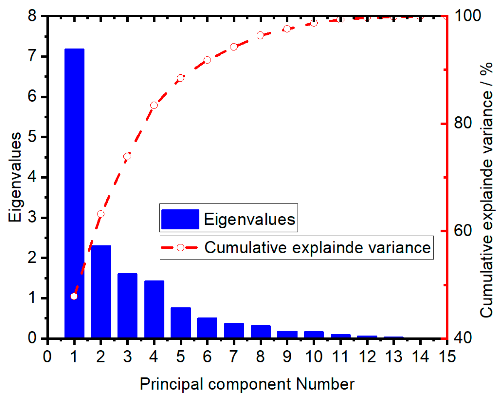
Because there is some correlation between the features, it is our intention to consolidate with closely related features into a minimal number of components, thereby ensuring that the resulting features are uncorrelated. This approach allows us to represent the various types of information present in each variable using a smaller number of composite features. Accordingly, following the completion of the principal component analysis (PCA) of the features, principal component analysis is a statistical method used to convert potentially correlated variables into linearly uncorrelated variables by orthogonal transformation, and these new variables are called principal components. The core idea of PCA is data dimensionality reduction, i.e., to reduce the dimensionality of data while retaining most of the information about these data. This was conducted for the purpose of reducing the dimensionality of the features, the principal component features, and the cumulative contribution graph is shown in Figure 6, where the selection of the principal components of the judgment conditions is the cumulative contribution of more than 85%.

After the principal component analysis, all motion segments were analyzed in a cluster analysis. The K-means clustering algorithm divides samples into different classes based on the distance of each parameter point to the cluster center. The distance calculation method chosen in this study was the Euclidean distance, shown in Equation (16).

$$d(X,C_i)=\sqrt{\sum _{j=1}^m{\left(X_j-C_{ij}\right)}^2}$$

(16)

where $d$ is the Euclidean distance, $X$ is the characteristic parameter point, $C_i$ is the ith clustering center, $m$ is the dimension of the parameter matrix, $X_j$ is the value of the jth attribute, and $C_{ij}$ is the value of the attribute of $C_i$.

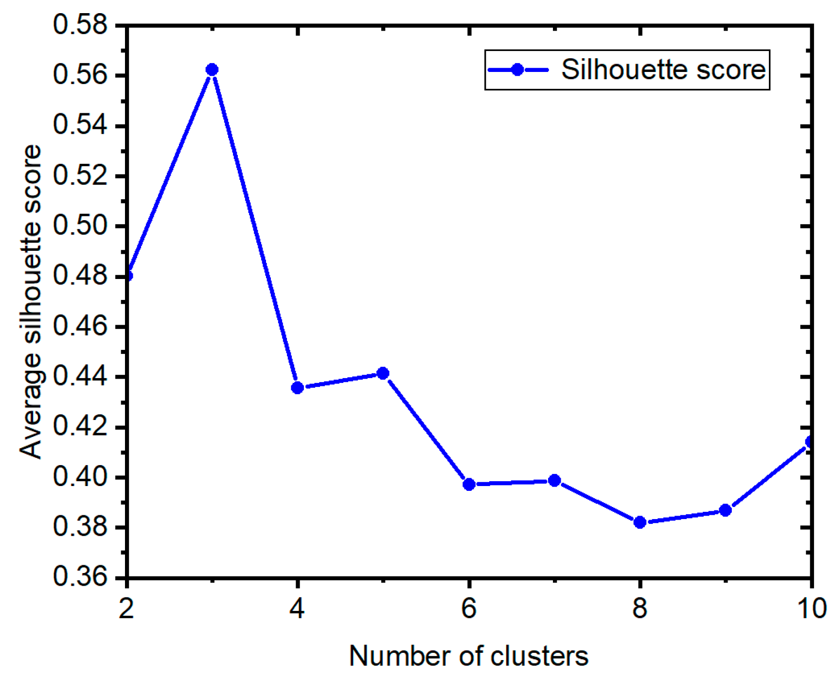
Prior to the implementation of clustering, it is necessary to ascertain the requisite number of cluster centers. This is achieved through the utilization of the silhouette contour function, which is employed to determine the optimal number of cluster centers. The different profile coefficients corresponding to k = [2, 10] are shown in Figure 7; as can be observed, the profile coefficients reach their maximum value for k = 3. Therefore, the number of clustering centers was set to three.

Then, based on the K-means algorithm, the clustering analysis was carried out for the two time periods of 08–09 h and 10–11 h and the 899 segments at 08–09 h were clustered into clusters of 288, 206, and 405, respectively, and the 88 segments at 10–11 h were clustered into clusters of 23, 39, and 26, respectively.

After the cluster analysis, the three conditions were divided into urban, suburban, and high-speed conditions to obtain the average value of each condition in the two typical traffic periods, and the comprehensive conditions were constructed according to the average value of each condition in the two typical traffic periods. Kinematic clips were spliced in a proportional no-playback random sampling of all types of working conditions under a total clip length of 5000, with mean values of 0.13, 0.34, and 0.53 for the percentage of working conditions at 08–09 a.m. on Monday–Friday, and mean values of 0.24, 0.29, and 0.47 for the percentage of working conditions at 09–10 a.m. on Monday–Friday. The number of kinematic segments of each category for the composite case is obtained as 8, 13, 12, 1, 3, and 2, and the constructed composite case is shown in Figure 8.

3.2. Hydrogen Consumption Minimization Strategy Based on PMP Solving

As posited by Pontryagin’s minimum principle, this study identified the fuel cell stack’s output power (P_fc) as the control variable. The state variable, on the other hand, was defined as the stack’s SOC. Finally, the performance index of the PMP algorithm was established as the hydrogen consumption of the entire vehicle.

The interdependence between $P_{fc}$ and $SOC$ is represented by the function $f$.

$$S\dot{O}C(t)=f(SOC(t),P_{\mathrm{dem}}(t),t)$$

(17)

The Hamiltonian function $H$ of the PMP method is shown in Equation (18):

$$H(SOC(t),P_{\mathrm{fc}}(t),\lambda (t),t)={\dot{m}}_{{\mathrm{H}}_2}(P_{\mathrm{fc}}(t))+\lambda (t)SOC(t)$$

(18)

where $\lambda$ is the covariate variable.

The initial term of the Hamiltonian function represents the real-time H₂ release rate of the fuel cell stack. The second term is the product of the rate of change in the state variable and the covariate, which is equivalent to the instantaneous rate of H₂ consumption by the power cell. $\lambda$ is the PMP algorithm; for a certain driving segment, different $\lambda$ values correspond to different energy allocation results, and finding the optimal λ when the energy allocation is optimal is the key problem to be solved by applying the PMP algorithm.

Boundary conditions must be set when executing a PMP policy, as in Equation (19).

$$S.t.\left\{\begin{array}{c}{P}_{fc\min }\le P_{fc}\le P_{fc\max }\\ -\Delta P_{fc\max }\le \Delta P_{fc}\le \Delta P_{fc\max }\\ P_{bat\min }\le P_{bat}\le P_{bat\max }\\ SO{C}_{\min }\le SOC\le SO{C}_{\max }\end{array}\right.$$

(19)

In pursuit of the goal of the best possible control, with due consideration of the boundary conditions, it is essential to identify the optimal control variable $P_{fc}$, with the objective of minimizing the Hamiltonian function $H$ on a time-by-time basis.

Therefore, the Hamiltonian function must fulfill the following three conditions.

$$\left\{\begin{array}{l}{\displaystyle \frac{\partial H}{\partial \lambda }}=s\dot{o}c\\ {\displaystyle \frac{\partial H}{\partial \lambda }}=s\dot{o}c\\ {\displaystyle \frac{\partial H}{\partial P_{\mathrm{fc}}}}=0\end{array}\right.$$

(20)

In accordance with Pontryagin’s minimum principle, the optimal $P_{fc}$ at each moment is given by the following equation.

$$P_{\mathrm{fc}}^{\mathrm{opt}}(t)=\arg min(H(t))$$

(21)

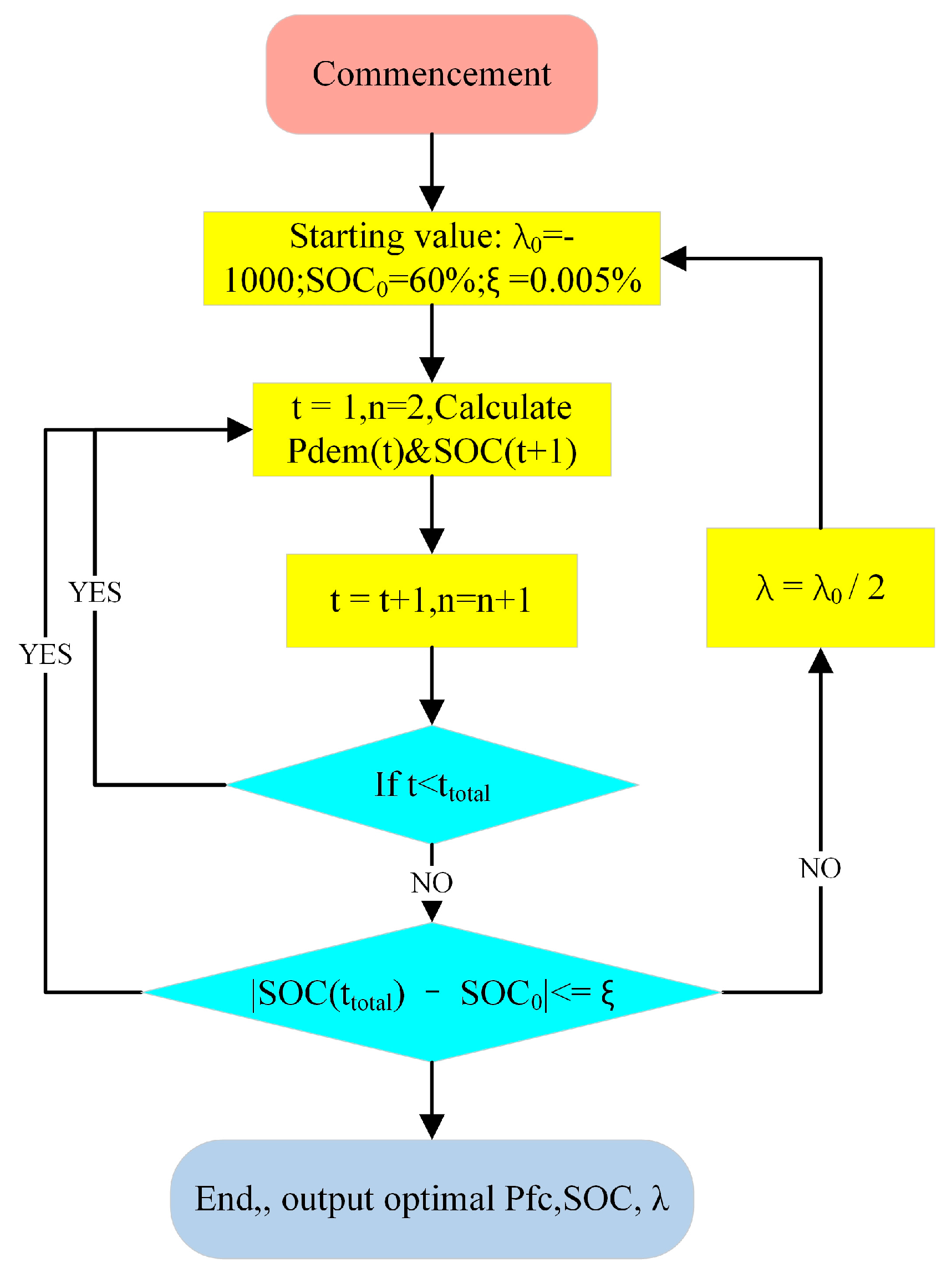
In conclusion, following the determination of the optimal λ, the optimum output energy of the system can be calculated by identifying the minima of the Hamilton function within each time step, in accordance with the principle of minimal perturbation. However, when considering different operational scenarios, the optimal λ is frequently found to vary and remain unknown. Therefore, it must be determined by an iterative search method. In this study, the optimal λ was solved iteratively using the target-hitting method. The specific solution flows are presented in Figure 9. The initial value of λ was set to −1000 in order to prevent solution leakage in the actual simulation.

3.3. Energy Management Strategies Based on Condition Identification

Covariates serve a pivotal function in energy allocation; the optimal covariates for each type of operating condition have been determined under historical conditions. In the driving segment with unknown conditions, the vehicle will apply the method proposed in this section to identify the conditions to obtain the online conditions containing different types of conditions and then allocate the energy to the identified different types of conditions by using the three typical condition covariates obtained under the historical conditions.

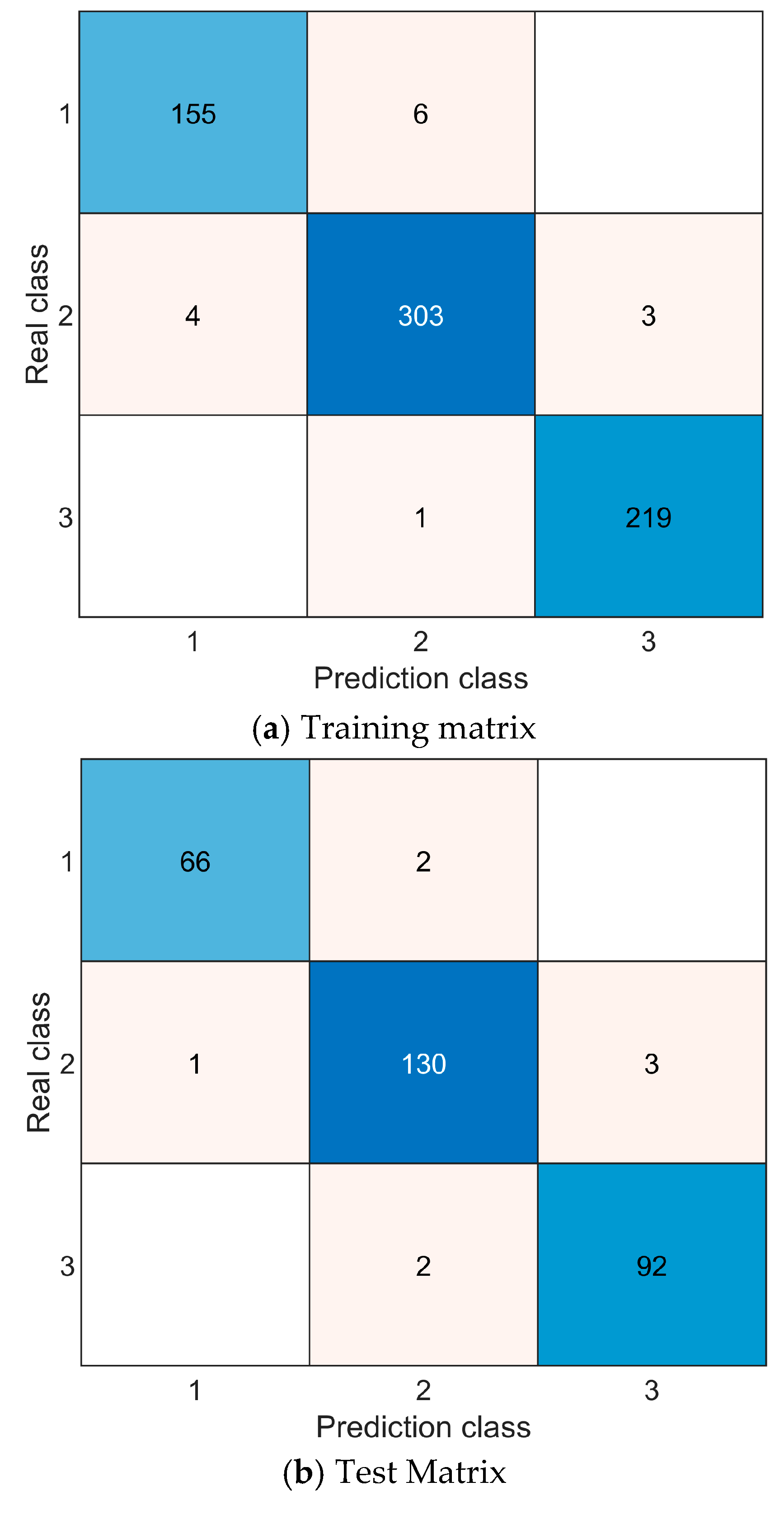
The total segments were divided into three categories after the cluster analysis, the labels of the clustered condition types corresponded to the total segments before the cluster analysis, and the construction of the offline model was carried out. In this study, we used the classification learner in the MATLAB toolbox for model construction, input the eigenvalues after principal component analysis as dataset variables and the segment categories after clustering as responses into the classification learner, and then utilized a variety of algorithms for model training. The linear Support Vector Machine SVM-trained model has the highest validation accuracy of 97.97%, while the test accuracy is 97.30%. Support Vector Machine is based on the theory of SVM statistical learning theory, which better solves the problems of nonlinearity, high dimensionality, local minima, etc. It does not involve probability measures and the law of large numbers and circumvents the traditional process from induction to deduction, and the classification result is determined by a few support vectors, which can “eliminate” a large number of redundant samples, making the algorithm simple and robust. The validation and test confusion matrices of the trained model are shown in Figure 10a,b.

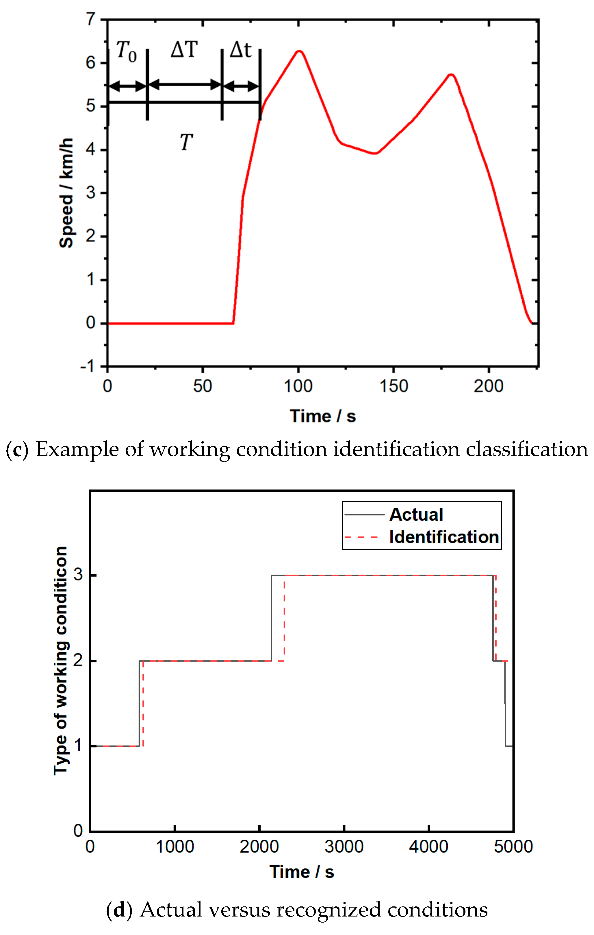
Online identification of integrated working conditions after completion of offline training model construction. The condition identification and update cycles are shown in Figure 10c. ∆T is the condition identification cycle, and ∆t is the condition update cycle. A comparison of the recognized working conditions with the actual working conditions is shown in Figure 10d, with an accuracy of 93.24%. The online recognition strategy uses the DBSCAN algorithm to identify historical driving segments that are similar to the current driving segment. The DBSCAN algorithm is an efficient density-based clustering algorithm. This algorithm categorizes samples based on how closely they are distributed, which is generally the case for similar samples. Then, the optimal λ is solved and determined through the application of the PMP strategy for energy management across the three historical working conditions of urban, suburban, and high-speed. The optimal λ is determined to correspond to the various identified working conditions, and subsequently, the power allocation and energy consumption are calculated for the entirety of the identified integrated working conditions.

3.4. Energy Management Strategy Based on Equivalent Consumption Minimization

Equivalent Management Systems (EMS) are a method of quantifying the energy consumption or carbon emissions of non-hydrogen energy systems (e.g., electricity, fossil fuels) into equivalent hydrogen consumption through the principle of energy equivalence. Regardless of the external energy input (e.g., brake energy recovery), the energy consumption of the hybrid system is ultimately provided by hydrogen. The Minimum Equivalent Hydrogen Consumption (MEHC) strategy, from the perspective of energy saving, equates electrical energy to the mass of hydrogen in the fuel. The equivalent hydrogen consumption strategy is to find the optimal equivalence factor (in this paper, it is a diagonal too variable) by calculating the minimum equivalent hydrogen consumption through optimization. Since the future working conditions are unknown, it is necessary to find the equivalence factor, so that the power cell is converted into the highest hydrogen consumption efficiency.

3.5. Energy Management Strategies Based on Time Classification

Since speed data from Monday to Friday from 08:00 a.m. to 09:00 a.m. and from 10:00 a.m. to 11:00 a.m. are processed to construct the working condition, the constructed working condition has the attribute of time. The optimal λ for each of the two time periods is calculated according to the PMP energy management strategy, and the current optimal λ is used in the current time period. In order to be closer to the real conditions, the online conditions are obtained by combining them with the condition identification, and the power allocation and equivalent consumption of the H₂ are calculated on the basis of the PMP energy management. In this way, the energy management strategy can be formulated on the basis of classification. The time-based classification method classifies data by the time on collected data, and then calculates the minimum hydrogen consumption of the data condition in whole hours, and then obtains the optimal slanting variables; in this paper, we adopt two time segments and thus two slanting variables, and each datapoint for the condition identified by a condition is associated with a time. We use the two slanting variables corresponding to the time segments through the time labels and then carry out the power allocation.

The proportion of each time period in the integrated conditions is shown in Figure 11, where the 08–09 a.m. time period accounts for 90.8% and the 10–11 a.m. time period accounts for 9.2%. After identifying the working conditions, the percentages of each working condition in the 08–09 time period are 12.73%, 34.34%, and 52.93%, respectively, and the percentages of each working condition in the 10–11 time period are 21.74%, 31.52%, and 46.74%, respectively.

The percentage of each time under the combined conditions is shown in Figure 11, with 90.8% for the 08–09 a.m. time and 9.2% for the 10–11 a.m. time. The percentages of all types of working conditions in the 08–09 a.m. time period after the identification of working conditions are 12.73%, 34.34%, and 52.93%, and the percentages of all types of working conditions in the 10–11 a.m. time period are 21.74%, 31.52%, and 46.74%, respectively.

4. Simulation Verification

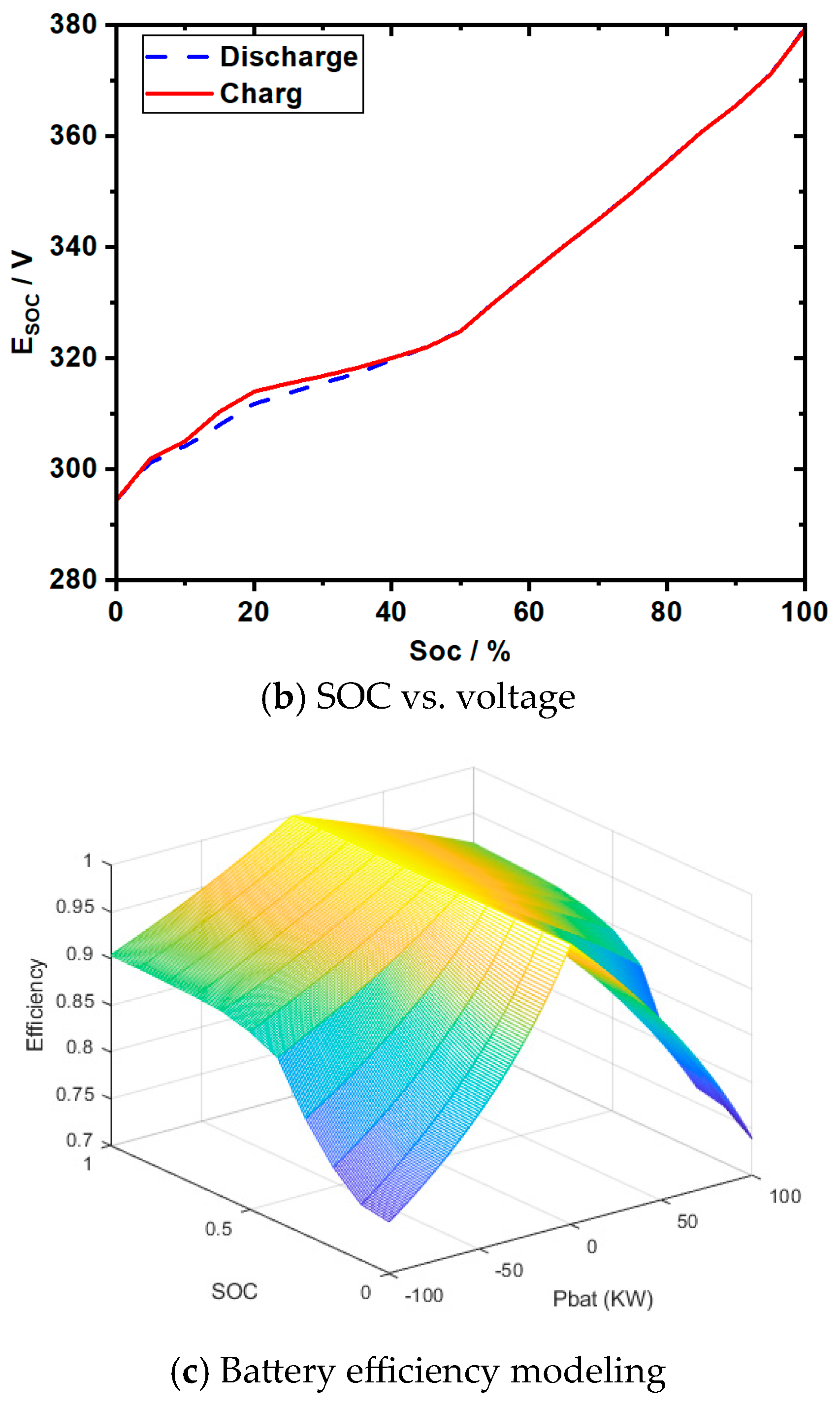
Before conducting the simulation, it is necessary to discuss the coordinated optimization of the battery charging and discharging efficiency with the fuel cell, especially the coordinated control strategy under different operating conditions. As shown in Figure 3c, a power battery efficiency model is established, i.e., battery efficiency versus SOC versus charging and discharging power, which is convenient to consider in conjunction with fuel cell efficiency. In some settings, the following considerations are made:

Priority discharge of the battery during rapid acceleration and high-power demand to protect the fuel cell life;

Fuel cell operating range setting to stabilize the fuel cell in the high-efficiency range;

Consideration of fuel cell power transient to extend fuel cell durability.

Design power battery charging and discharging SOC interval in [0.2,0.8], in order to protect the power battery life, the design of the battery power interval Pbat = [−10,70], thus limiting the power battery efficiency interval, which furthers the battery and fuel belt consumption efficiency of the synergistic calculation toward the optimal setting;

For different working conditions, it is necessary to set some limitations for coordinated control of the fuel cell and power cell:

In urban areas, idling, frequent start-stop, low power demand, fuel cell shutdown, or low power state result in the main power being supplied by the power battery, and during rapid acceleration, the power battery provides peak power (=<70 kw).

In suburban working conditions, the vehicle speed moves at a medium speed, driving smoothly; the fuel cell is in the high-efficiency range, with a small range of battery charging as well as energy recovery, the maximum charging power or recovery power of 10 kw, and the peak power is provided by the battery during rapid acceleration.

In high-speed conditions, the vehicle travels at high speed with continuous high-power demand; the fuel cell works in a high-power range during rapid acceleration or overtaking, and the battery provides short-term peak power support. Less than or equal to 10 kw at energy recovery.

To ascertain the efficacy of the time-classified energy management strategy under investigation, a series of comprehensive test conditions were selected for simulation and analysis purposes. The FCS+PB hybrid vehicle model was constructed in MATLAB/SIMLINK(2022b), and the working conditions were imported and simulated according to the specified control strategy. The calculation and analysis of equal consumption of H₂ of the entire vehicle is carried out based on the comprehensive test conditions to compare the economic performance of the strategy based on the identification of the working conditions with that of the strategy based on time classification.

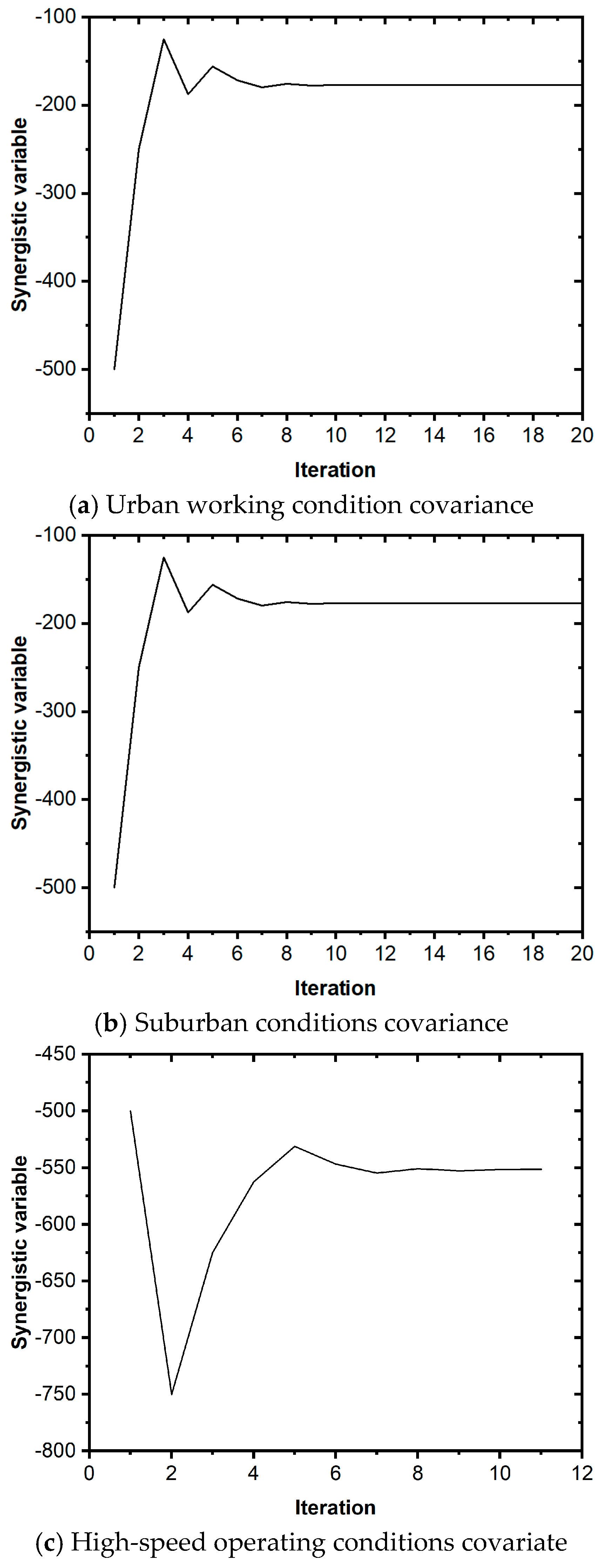
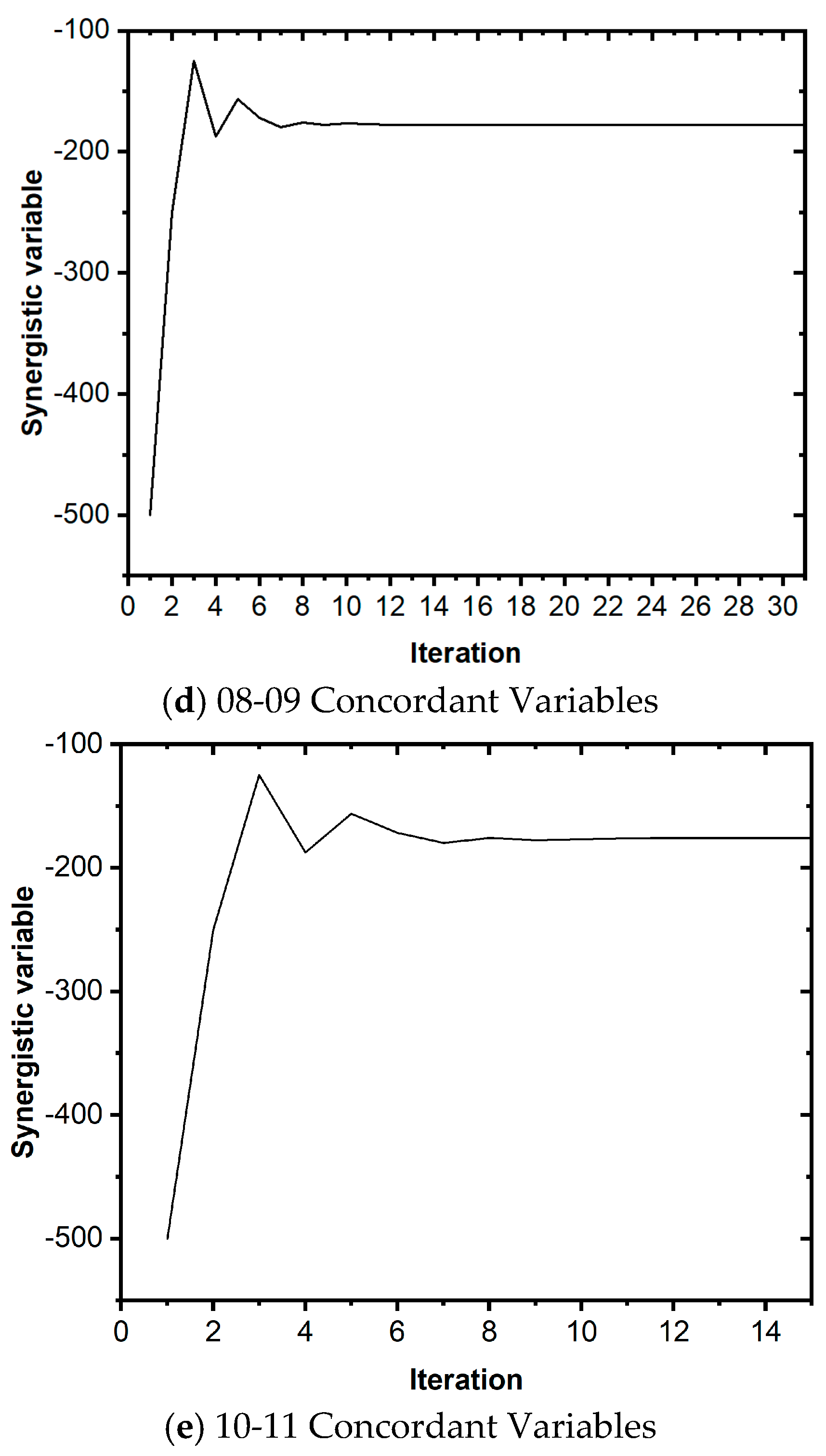
In order to verify the strategy implementation and credibility of the simulation software, we analyze the iterative solutions of the “dichotomous” method for the optimal ramp variables, power allocation, equivalent hydrogen consumption, and battery SOC output. Figure 12 shows the optimal λ solving iterations for three typical operating conditions and two time periods in urban, suburban, and highway areas, and the iterations are stopped when the iteration conditions are satisfied. The results show that the iteration speed of the target localization method is related to the amount of data, and the larger the amount of data, the slower the iteration speed. However, there is a sudden jump effect in the iteration process, which successfully jumps out of the local extremes.

Following an iterative optimization search to identify the global optimal covariates for three typical operating conditions and two time periods, the PMP can convert the global optimization challenge into an instance of instantaneous optimization. The optimal fuel cell system output power can be obtained by identifying a minimal solution to the Hamiltonian function at each time step, which is computationally small and has potential for real-time applications.

As seen in Figure 12c, although the dichotomous logic is used, the discretization takes values such that the synergistic variables are decreasing in fixed steps. The process reflects the adaptive tuning of the dichotomy method under a limited number of candidate values and finally succeeds in locating the optimal value of the equivalent hydrogen consumption −800. The higher number of iterations (12) may originate from the reduced convergence efficiency because of the discretization. In contrast, in the other plots in Figure 12, the iterative graphs reflect a wider search range or finer discretization step sizes, resulting in an increased number of iterations. The core difference lies in the discretization strategy and the setting of the initial interval, which highlights the flexibility and efficiency limitations of the dichotomy method under discrete constraints. Under more stringent hydrogen consumption requirements or higher accuracy demands, the process of the dichotomous method adapts to the discretization constraints by increasing the number of iterations to approach the target value, highlighting the robustness of the algorithm under the finite candidate value and the computational cost trade-off.

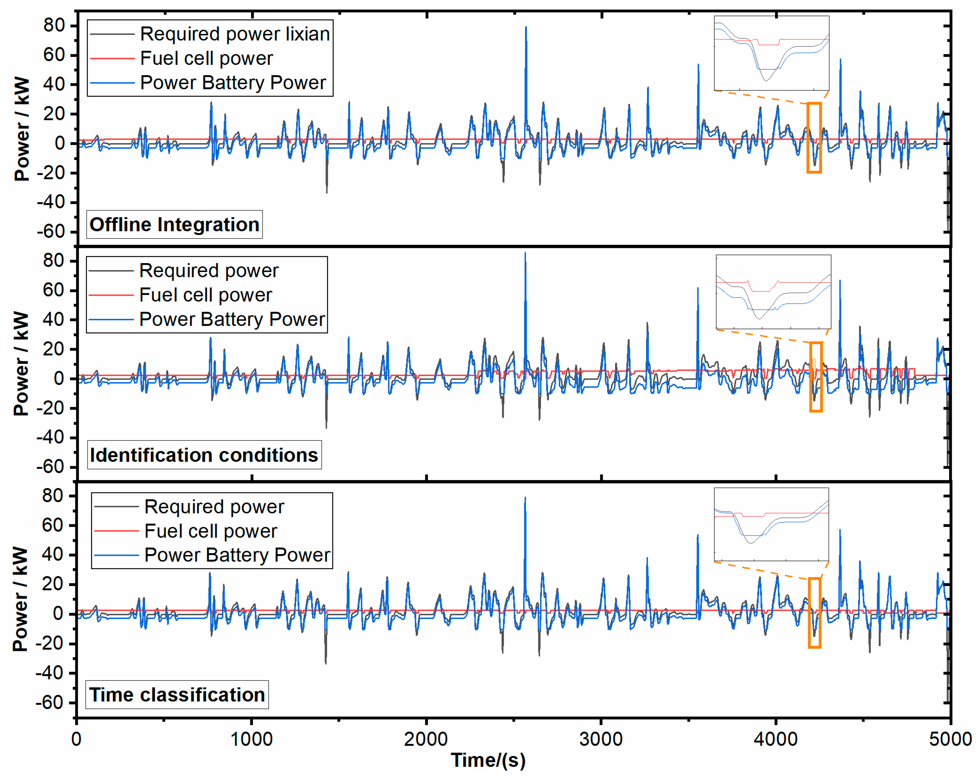
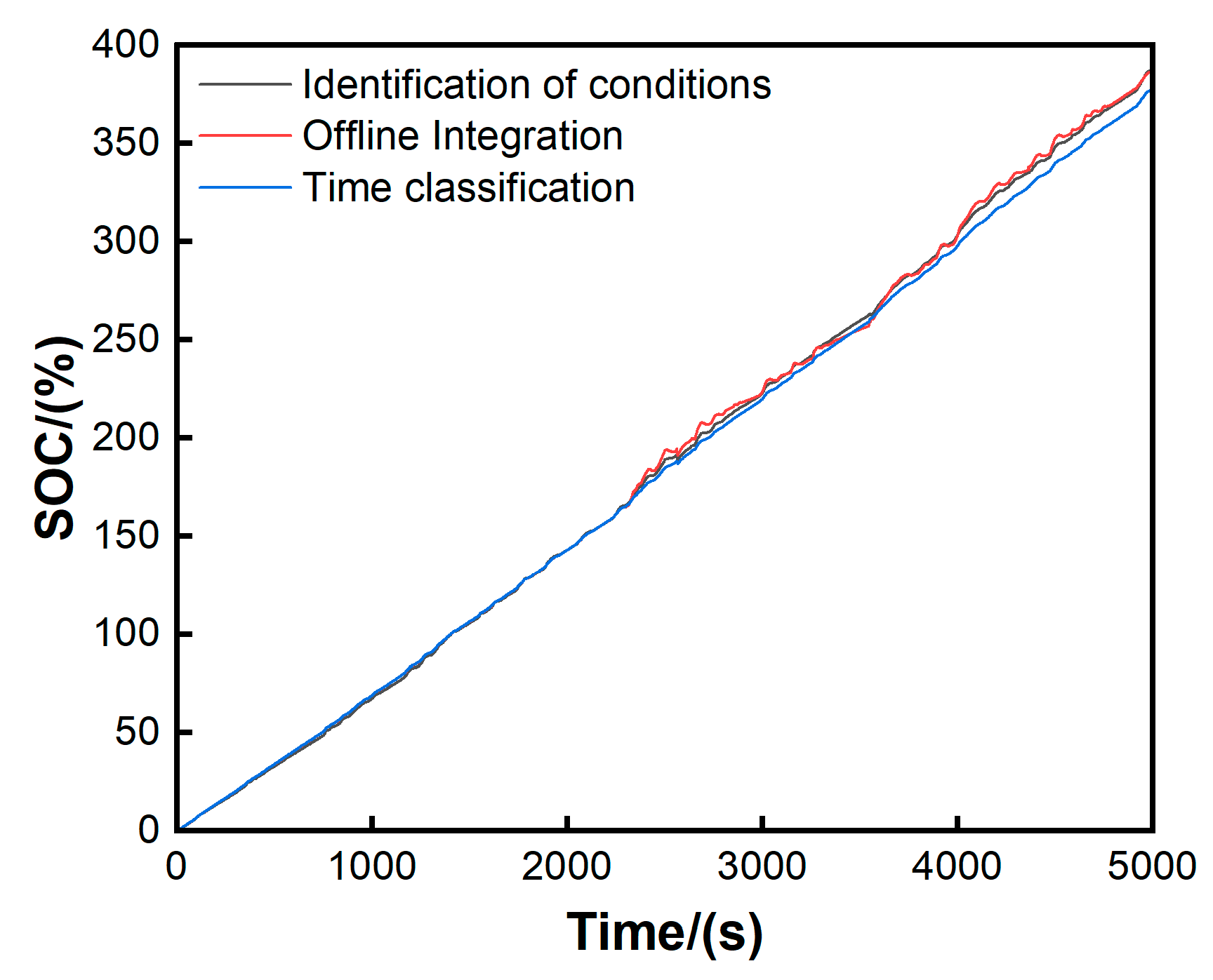
The outcomes of power allocation as determined by the PMP strategy simulation for the offline integrated conditions, condition identification, and time classification are illustrated in Figure 13. As illustrated in the figure, the simulation of the PMP strategy for offline conditions demonstrates that the output power of the fuel cell system is consistently maintained at a fixed value, closely following the power demand with minimal fluctuations. Conversely, the power cell exhibits a more pronounced variation in response to fluctuations in the power demand. The SOC variations were consistent with the solution constraints.

Figure 13 shows the power allocation results of the three strategies: the first power allocation result is the power allocation result in the offline state, the second is the power allocation result of the working condition identification strategy, and the third is the power allocation result of the time classification strategy. All strategies need to dynamically allocate power between the fuel cell and the power cell to match the real-time demand. Fuel cell stable output: under offline conditions, the fuel cell power maintains a fixed value with only small fluctuations to assume the base load, reflecting its adaptability to steady state demand, and the optimal fixed power of the fuel cell is determined through global optimization to minimize hydrogen consumption while constraining the SOC changes. Working condition identification: the control parameters are dynamically adjusted according to working condition segments (e.g., acceleration, cruise, braking), which is consistent with the segmentation logic in the time classification strategy. Power Battery Response Fluctuation: power battery power varies with demand at high frequency (e.g., ±60 kW) and is responsible for absorbing or replenishing transient power shortfalls, consistent with the dynamic balancing logic in the hybrid strategy.

As illustrated in Figure 12, the absolute value of the power supply and demand in the simulation results of the PMP strategy based on the working condition identification strategy is greater than that of the offline working condition. As illustrated in Figure 10c, the recognition accuracy is not 100%. This results in some conditions being incorrectly identified, with the majority of these errors occurring at the point of alternation in condition changes. This is a consequence of the inclusion of two distinct types of condition information. The covariate can be conceptualized as a penalty factor that influences changes in the rate of change in SOC. As illustrated in Figure 14a, when the covariate increases, the objective is to minimize the Hamiltonian function, which results in the system discharging the energy storage cell and reducing the SOC. Conversely, when the covariate decreases, the system is driven to charge the energy storage cell, thereby increasing the SOC. Some of the high-speed conditions and urban areas were identified as suburban conditions, and the percentage was much higher than the proportion of suburban conditions identified as urban areas, while both high-speed conditions and urban areas were identified as suburban conditions that increased $\lambda$ larger, which led to a higher overall discharge of the comprehensive test conditions, resulting in a decrease in SOC. This results in the power allocation, and in Figure 14b, the SOC varies less in the early period compared with the offline condition, while in the later period, the rate of change becomes larger when the high-speed condition is recognized as a suburban condition. Furthermore, the discrepancy in the SOC between the initial and final stages is more pronounced in comparison to the offline scenario.

The time-based classification strategy uses the current time covariate at the current moment λ, and $\lambda$₁₁ = −175.88, $\lambda$₂₂ = −177.67 for the current two times. Owing to the time-based classification strategy, both offline and online working conditions use different λ values under different working conditions. As illustrated in Figure 14, λ follows the working conditions of −176.81, −176.71, −551.45, −551.45, −176.71, and −176.81, respectively; the first three operating times correspond to λ₁₁, which are all higher than the three different operating conditions λ in time, so the SOC decreases. The last three working conditions time corresponds to λ₂₂, where λ₂₂ is higher than the time within the high-speed working conditions λ, but lower than the λ of the suburban open and urban conditions; thus, the SOC first decreases and then increases, and the first and last SOC difference is larger than the offline condition. Given the similarity between the SOC time-based classification strategy and the offline condition, the power allocation is also analogous. Consequently, the discrepancy between the power cell power and the power demand is diminished, as is the fuel cell output power.

As can be seen from the hydrogen consumption plots for the three conditions in Figure 15, the time-based classification strategy has the lowest hydrogen consumption, whereas there is not much difference between the offline condition and the work recognition hydrogen consumption, which is due to the fact that the recognition accuracy is not 100% during the recognition process.

A comparative analysis of the analogous findings pertaining to the consumption of equivalent hydrogen is presented in

Table 4. Equivalent hydrogen consumption for three strategies.

Energy Management Strategy	Equivalent Hydrogen Consumption/g	Reduction Rate Compared with Offline Combined Operating Conditions/%
Offline comprehensive working conditions	387.2	-
Work condition recognition	387.6	0.103
Time classification	376.72	2.707

, which is based on the primary cycle condition and encompasses the three strategies under consideration.

As evidenced by Table 4, the comprehensive test conditions reveal that the equal consumption of H₂ in the energy management strategy grounded in condition identification is diminished by a mere 0.103% because of the suboptimal accuracy. In contrast, the equal consumption of H₂ in the energy management strategy anchored in time classification is reduced by 2.707%, a notable enhancement that considerably optimizes the economic efficiency of the entire vehicle.

To further compare the economic advantages of the optimal strategy, 10 simulation cycles were performed based on comprehensive operating conditions. The time-based classification strategy, which requires 3758 g of equivalent hydrogen, resulted in a 3.788% reduction in equivalent hydrogen consumption compared with the condition-based identification strategy, which required 3899 g.

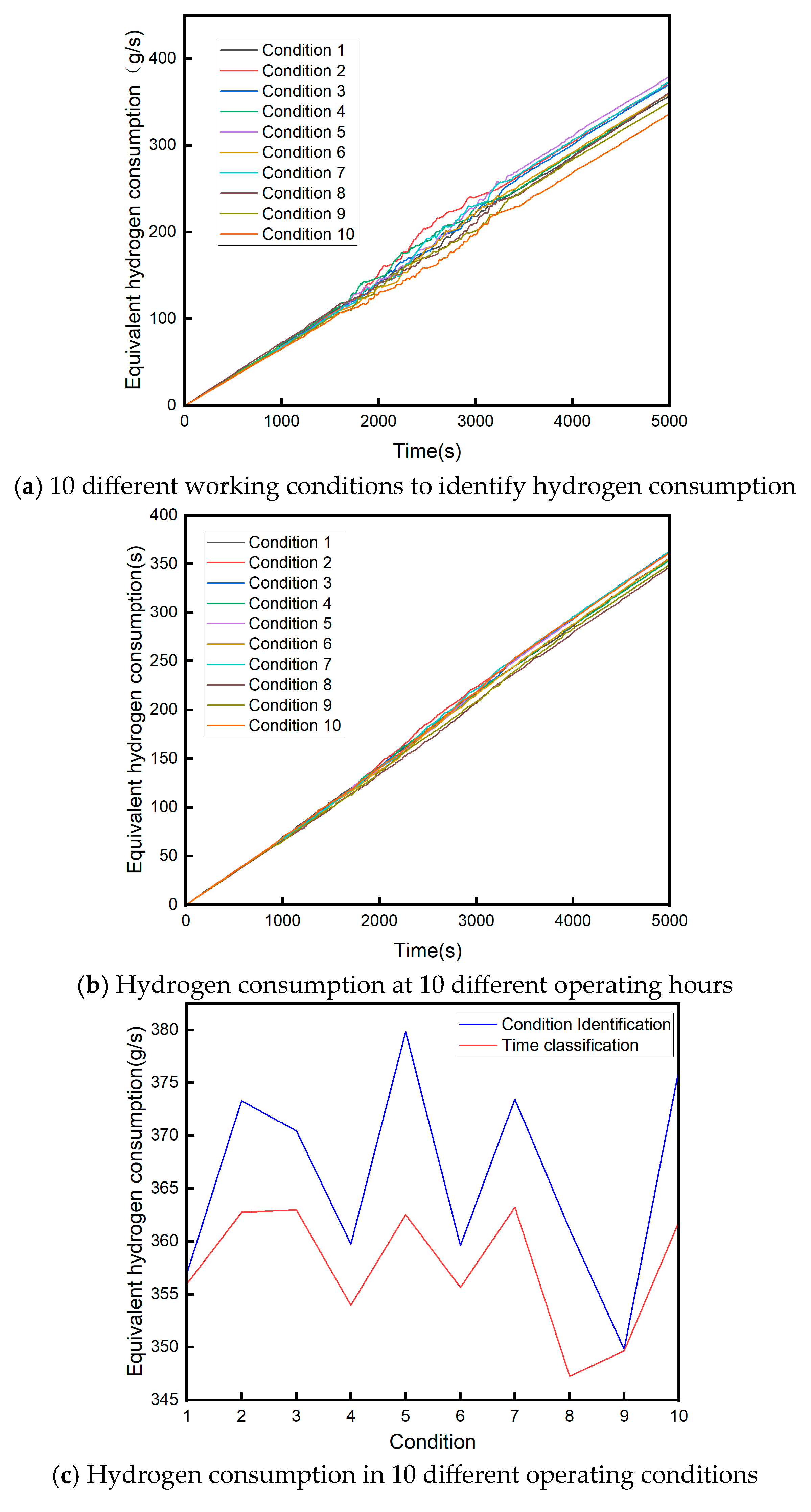
In order to further verify the effectiveness of the strategy, we constructed 10 working conditions to analyze the two strategies statistically and established an independent samples t-test to analyze and compare the difference in the mean values of the hydrogen consumption data of the two strategies under 10 working conditions. First, we plotted the variation in hydrogen consumption for the condition identification and time classification strategies, as shown in Figure 16. Figure 16a shows the variation in hydrogen consumption for 10 different conditions calculated by the condition identification strategy, and Figure 16b shows the variation in hydrogen consumption for 10 different conditions corresponding to the time classification strategy. From the two plots, it can be seen that the fluctuation in the middle portion of the curve is obvious, which is due to being in the high-speed stage, which requires a high power output, whereas the curve is stable in the low–medium-speed stage, which conforms to the low–medium-speed stage, and the curve is stable in the medium-speed stage, which conforms to the low–medium-speed stage. This occurs because the high-speed stage requires high power output, while the low and medium-speed stages have stable curves in line with the low and medium power cases. In the comparison of the two strategies, the stability of the time classification strategy is obviously better, with less fluctuation, which is suitable for dynamic change scenarios.

The comparison of the hydrogen consumption results for the last 10 different conditions is shown in Figure 16c. The hydrogen consumption of the time classification strategy is lower than the condition identification; the difference between the two is as low as 0.1736 g for the ninth condition and as high as 17.3186 g for the fifth condition. We then performed independent t-tests on these 20 hydrogen consumption values.

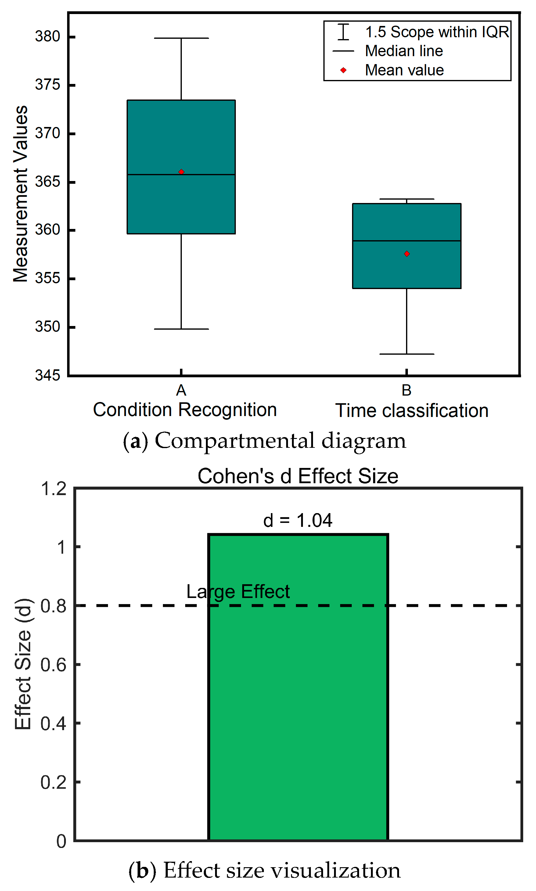
Finally, statistical analysis and hypothesis testing were performed on both sets of data.

Table 5. Results of descriptive statistics.

Groups	Mean ± Standard Deviation	Standard Error (SEM)
Condition identification	366.06 ± 10.21	3.23
Time classification	357.58 ± 5.90	1.86

Descriptive statistics results.

The normality test was performed: p1 = 0.372, p2 = 0.415, and both groups of data conformed to a normal distribution (p > 0.05);

Chi-square test: Levene’s test p = 0.123, hypothesis is valid (p > 0.05);

Independent samples t-test: t(18) = 2.25, p = 0.037, 95% CI [0.57, 16.39], from Figure 17b, Cohen’s d = 1.04 Difference between the two groups was statistically significant (p < 0.05) and had a large effect size (d > 0.8);

The above results show that Group Y is significantly better than Group X in terms of treatment effect and its equivalent hydrogen consumption is lower, and the difference is practically significant (d > 0.8). The experimental conclusions support the strategy of prioritizing Group Y in dynamic or steady-state scenarios to optimize the efficiency of hydrogen energy utilization.

5. Conclusions

This study develops hybrid vehicle models integrating fuel cells and energy cells, analyzing their structural and energy flow characteristics. Time classification-based energy management strategies are designed to optimize power allocation under identified operating conditions, with the following key findings:

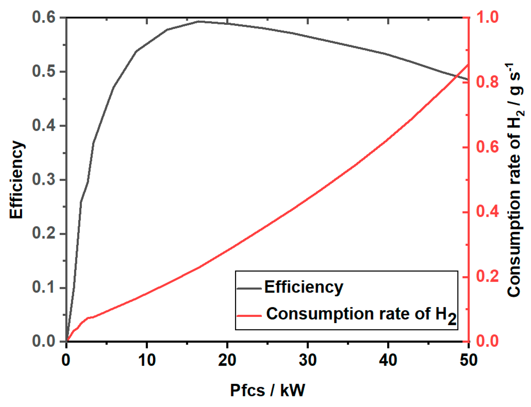
The fuel cell system exhibits limited dynamic responsiveness to minor power fluctuations, while the energy cell adapts better to significant power shifts. Efficiency models for both components are critical: battery charging/discharging efficiency decreases notably with rising power demand, and fuel cell efficiency varies nonlinearly with internal stack consumption and output power. Establishing these efficiency models is essential for system optimization.

Analysis of PMP-based energy management strategies reveals that higher covariate values (λ) prioritize battery discharging to minimize the Hamiltonian function, reducing SOC. Conversely, lower λ values favor battery charging to elevate SOC. This principle governs SOC dynamics across all tested strategies, including condition-adaptive PMP approaches.

MATLAB simulations demonstrate that the proposed time classification strategy achieves superior power distribution, reducing equivalent hydrogen consumption by 6.2% compared with offline PMP strategies while maintaining dynamic performance. Over 10-cycle testing, this approach enhances the vehicle’s range by 12–15% and improves overall economic efficiency, validating its effectiveness in balancing energy utilization and operational costs.

Hydrogen consumption issues were not considered along with lifetime shortening and performance degradation during the modeling process. However, X Tang et al. developed a reliable model for effectively monitoring the dynamic decay behavior of proton exchange membrane fuel cell stacks with respect to the state of health (SOH) and voltage decay of fuel cell stacks (FCSs) [26]. Their study lays the foundation for a paper to explore further and improve the relationship between hydrogen consumption, lifetime shortening, and performance degradation, and to more closely match the actual conditions.

This study has achieved milestones in the exploration of energy management strategies for fuel cell hybrid vehicles, but there are still the following limitations that need to be explained: the dynamic aging characteristics of the fuel cell electric stack are ignored, assuming that the performance of the fuel cell is constant; the influence of the ambient temperature on the energy management system (which includes components such as the fuel cell), and the thermal management system has not been included; and the lack of test experiments on real vehicles, and the energy management strategy was carried out on simulation software and not applied to real vehicle testing.